1. Introduction
Forests are the largest terrestrial ecosystem on Earth, and they play an irreplaceable role in the carbon cycle and sustainable development [
1]. The vertical structure of a forest not only directly reflects the growth and development of the forest, but is also an important and necessary input for estimating above-ground biomass and storage [
2,
3,
4]. Since interferometric synthetic aperture radar (InSAR) can provide penetrability into forest, especially in the long wavelengths such as the L-band and P-band, it has become an invaluable tool for vertical structure reconstruction over forest areas. However, it cannot discriminate the different scatterers within one resolution cell, and the estimated height is the mean of all the scatterers’ heights.
Synthetic aperture radar tomography (TomoSAR), which is a new advanced SAR technique, can solve this problem because it has the vertical resolution to achieve three-dimensional imaging. TomoSAR has been widely applied over forest areas to acquire the vertical structure [
5,
6]. The idea behind the concept of TomoSAR is that it combines multiple acquisitions to form an additional synthetic aperture along the vertical direction, in addition to the conventional aperture along the azimuth direction [
7,
8].
In order to obtain a nice tomogram, many SAR images with uniformly distributed baselines are required for tomographic focusing [
9,
10,
11,
12,
13,
14,
15,
16,
17,
18]. However, it is usually impossible to obtain enough images with uniformly distributed baselines in every area. Thus, there are two difficulties for TomoSAR [
19,
20,
21]: (1) For a small number of acquisitions, the common Fourier-based TomoSAR focusing approaches bring about some imaging quality problems [
22,
23]. If we want to get a good tomographic focusing, we have to acquire more images. However, this would require more flights for an airborne sensor or more repeat orbits for a spaceborne platform, which would greatly increase the cost of the data acquisition. (2) The non-uniformly distributed baselines mean that the observations are non-uniformly sampled in space. To address the non-uniform sampling problem, it is common to carry out interpolation to obtain uniformly sampled observations. However, this processing is sensitive to noise and may cause some other error. In summary, there is an urgent need to achieve high-quality tomographic focusing in the case of a small number of non-uniformly distributed acquisitions.
In order to solve this problem, compressive sensing (CS)-based TomoSAR has been proposed [
22,
23,
24,
25,
26,
27,
28,
29,
30,
31]. CS, as a sparse estimation technique, breaks the limitation of Shannon’s sampling theorem when the signal is compressible or sparse in a transform domain [
22,
23,
24,
25,
26,
27,
28]. It can not only greatly reduce the cost of the data acquisition, but also effectively overcomes the limitation of non-uniformly distributed baselines. Moreover, CS has a very high resolution along the vertical direction. However, CS based on convex optimization solvers such as the CVX solver requires the user to select a hyperparameter that closely depends on the noise of a pixel. And this hyperparameter directly affects the performance of CS. In general, if the value of the hyperparameter is too small, it can lead to overfitting, whereas a too large value can lead to underfitting.
In this paper, to overcome this limitation, we propose the use of the sparse iterative covariance-based estimation (SPICE) approach in TomoSAR for application in forest areas. SPICE, as a new sparse spectral estimation approach, follows the framework of the sparse estimation theorem. Accordingly, SPICE has the same advantages as CS. Moreover, SPICE exploits the minimization of a covariance matrix fitting criterion to address the sparse parameter estimation, taking account of the noise in every pixel adaptively. This successfully avoids the difficulty of selecting a hyperparameter [
32,
33,
34]. However, the backscattered reflectivity along the vertical direction over forest areas is continuous. Thus, the SPICE algorithm cannot be directly applied in tomographic focusing over forest areas. To address this issue, we use the wavelet and orthogonal (W&O) sparse basis to perform sparse expression of the forest signal. The used sparse basis not only ensures the sparsity of the forest canopy scattering contribution, but it can also keep the original sparse information of the ground scattering contribution. For the sake of simplification, this method is named W&O-SPICE in this paper. After making the forest backscattered reflectivity power sparse, the SPICE algorithm can be used in tomographic focusing.
The objective of this paper is to develop a hyperparameter-free sparse spectral estimation method, which can provide high vertical resolution in the case of a small number of non-uniformly distributed acquisitions for the application of TomoSAR over forest areas. The rest of this paper is organized as follows.
Section 2 first gives a brief introduction to the TomoSAR imaging model for sparse spectral estimation. The W&O sparse basis and the W&O-SPICE method are then explained.
Section 3 describes and analyzes the results of the simulated experiments.
Section 4 describes the study area and datasets, presents the tomograms in three polarizations, provides the estimated underlying topography and forest height obtained with three fully polarimetric P-band F-SAR airborne images, and describes the evaluation of the results with LiDAR measurements. A further discussion about the differences between SPICE and other TomoSAR methods is given in
Section 5. Finally, our conclusions are drawn in
Section 6.
2. Methodology
2.1. The TomoSAR Imaging Model for Sparse Spectral Estimation
After obtaining a stack of
N multiple-baseline SAR images over the same area, it is necessary to do some preprocessing steps, including selecting the master image, co-registration, deramping, and phase calibration. The focused complex value
at an arbitrary pixel of the
nth image can then be expressed as follows [
7,
8]:
where
denotes the complex scattering coefficients along the vertical direction,
is the vertical wavenumber of the
nth image with respect to the master track,
is the perpendicular baseline of the
nth image,
is the wavelength,
r is the slant range, and
is the incidence angle.
Through discretizing the continuous reflectivity function along the vertical direction
z by
D intervals, the imaging model (Equation (1)) can be approximately written as [
7,
8]:
where
g
is the vector of the
N observation measurements,
is the unknown discrete reflectivity vector with
D elements, and
.
e is the noise vector containing
N elements.
A is named the steering matrix with
, and the steering vector
given by:
where
T denotes the transpose operator.
However, over forest areas, Equation (2) is not a linear sparse model and we cannot directly apply sparse spectral estimation methods like CS and SPICE to do tomographic focusing.
If we assume that the temporal decorrelation can be ignored, then the covariance matrix of multiple SAR observations
g can be expressed as [
22,
28,
29,
30]:
where
is the expectation operator.
denotes the conjugate transpose.
P is the weight matrix, and
.
is the unknown noise power.
In fact, Equation (4) is a linear expression, as follows [
22,
28]:
where
y and
is a vector with
elements;
B is a
coefficient matrix; and
p is a vector with
D reflectivity powers. Specifically:
where
.
is the sample data covariance matrix with
.
K is the number of looks.
is the
mth column vector of steering matrix
A, and
is the
nth column vector of steering matrix
A. ⨀ indicates element-wise multiplication.
When a sparse basis is used to make reflectivity power vector
p sparse, Equation (5) becomes a linear sparse model. Thus, we can use spectral estimation methods like CS to do tomographic focusing [
22,
28,
29,
30]. Moreover, for the application of TomoSAR over forest areas, the parameters of interest are the reflectivity powers along the vertical direction
, rather than the complex reflectivity
.
2.2. W&O Sparse Basis
Over forest areas, the reflectivity powers along the vertical direction are not sparse. Thus, we cannot directly apply SPICE estimator to do tomographic focusing. One effective solution is to make the vertical reflectivity power sparse.
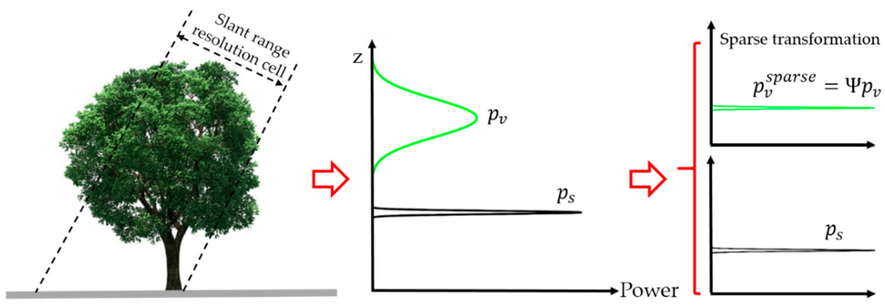
The reflectivity power is usually regarded as being contributed from both the ground and canopy, as shown in
Figure 1. For the ground backscattering reflectivity power
, its corresponding spectrum along the vertical direction has an isolated narrow peak and a very small angular spreading, like a point-like signal [
35], as shown in the black line in
Figure 1. As for the canopy backscattering reflectivity power
, its corresponding spectrum along the vertical direction has a wide angular spreading, which is much larger than the vertical resolution (the green line in the middle of
Figure 1). Thus, the ground backscattering reflectivity power
can be considered as sparse, while the canopy backscattering reflectivity power
can be considered as non-sparse.
In this paper, the wavelet basis
Ψ and unit orthogonal basis
I (W&O) are used to perform the sparse expression [
30]. The W&O sparse basis can not only ensure the sparsity of the forest canopy scattering contribution, but it can also keep the original sparse information of the ground contribution. This also makes up for the shortcoming of the conventional wavelet basis, i.e., the sparseness of the ground backscattering contribution is weak, especially for the strong ground contribution.
2.3. W&O-SPICE TomoSAR Method
SPICE, as a sparse spectral estimator, has a simple and sound statistical foundation, and takes account of the noise in a natural manner. Furthermore, it does not require the user to make a difficult selection of a hyperparameter [
32,
33,
34].
From the analysis in
Section 2.2, Equation (5) can be written as:
where
is the coefficient matrix of the canopy contribution and
is the coefficient matrix of the ground contribution
is the canopy backscattering reflectivity power in the sparse domain with
L elements.
Equation (7) can be rewritten as:
where
is the new mapping matrix.
.
is the canopy reflectivity power in the sparse domain and
is the ground reflectivity power. Moreover, a few elements of x are different from zero and
.
From the above analysis, Equation (8) is a sparse linear model, which is essentially the same as the application model of SPICE in References [
32,
33,
34]. Moreover,
y is the vectorization of data sample covariance matrix, which means that
y is obtained with the single look. Thus, the SPICE algorithm in the case of single look [
32,
33,
34] can be used to estimate the unknown parameters
x in Equation (8).
Equation (8) can be rewritten as follows [
32,
33,
34]:
where
;
.
For the case of single look, the estimation metric of SPICE is the following weighted covariance fitting criterion [
32,
33,
34]:
where f is the cost function;
stands for the Frobenius norm of the matrices.
is the Hermitian positive definite square root of
.
R is the modeled covariance matrix of
y.
According to References [
32,
33,
34],
R can be expressed as:
where
is the weight matrix, which can be expressed by:
where
are the canopy contributions in the sparse domain and
are the ground contributions.
are the noise contributions.
The solution to the minimization of the cost function f is equal to the minimization of the following equation [
34]:
where
.
is the
dth (
) column vector of matrix
.
Through solving Equation (13), the unknown sparse reflectivity power parameters
can be estimated. After that, we can use the sparse basis to obtain the real forest backscattering reflectivity power
p in Equation (5), as follows:
The following
Table 1 presents the detailed processes of the SPICE algorithm [
34]:
- (1)
Calculate the initial value according to and , where is the dth column vector of matrix .
- (2)
Calculate every unknown parameter’s power in the ith iteration.
- (3)
Calculate every unknown parameter in the ith iteration.
- (4)
Calculate the weight matrix in the ith iteration.
- (5)
Calculate the covariance matrix R in the ith iteration.
- (6)
Calculate the convergence of the last two iterations . If this value is less than , the iteration process is terminated; if not, the iteration process continues.
3. Simulation Experiments
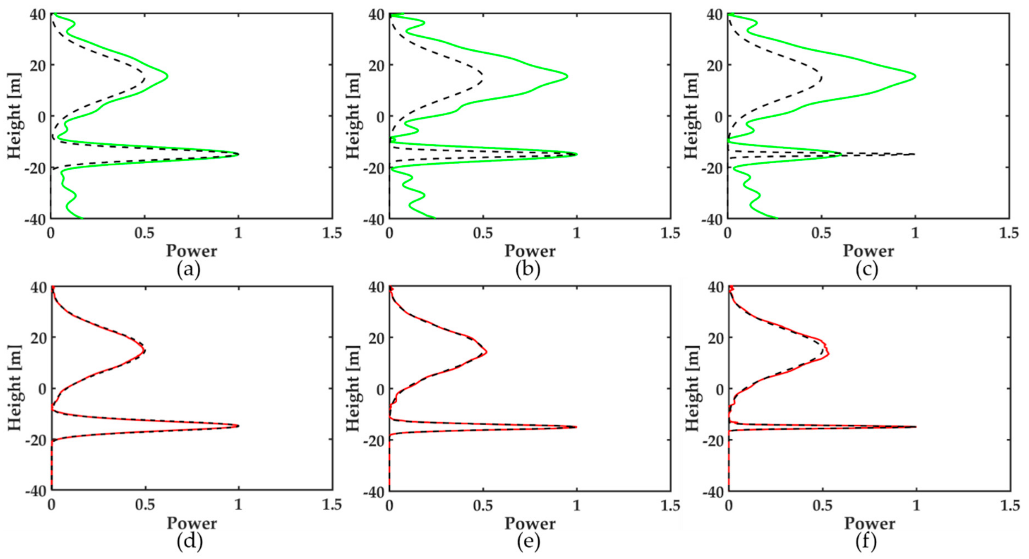
In order to demonstrate the feasibility and effectiveness of the proposed method, a set of simulation experiments was carried out. Due to the influence of the imaging wavelength, polarization mode, forest density, and species, different types of forest have different scattering characteristics [
35]. Considering this point, we simulated three kinds of forest scattering scenarios: (1) r > 1, where the ground scattering dominates, and r is the power ratio between the ground scattering and the canopy scattering; (2) r = 1, where the ground scattering power is equal to the canopy scattering power; and (3) r < 1, where the canopy scattering is dominant. The wavelength, slant distance, and other parameters used in the simulation experiments are listed in
Table 2. The tomographic focusing profiles were acquired from three aspects:
- (1)
The reconstruction performance of SPICE based on the wavelet basis and W&O basis, respectively, was investigated in the case of the same angular spreading with different kind of forest scattering scenarios.
- (2)
The reconstruction performance of CS based on the W&O basis was investigated with different selected hyperparameter in the case of the same forest scattering scenario (r > 1).
- (3)
We then compared the reconstruction performance between CS and SPICE with different ground angular spreading in the case of the same forest scattering scenario (r > 1).
Considering the implementation facility and compactness to solve the
L1-norm minimization [
23,
24,
25,
26,
27,
28,
29,
30], this paper applies the CVX solver for the CS TomoSAR method. The hyperparameter is set as 1000, which is an appropriate choice.
Based on the results of the above simulations, a number of observations can be made:
- (1)
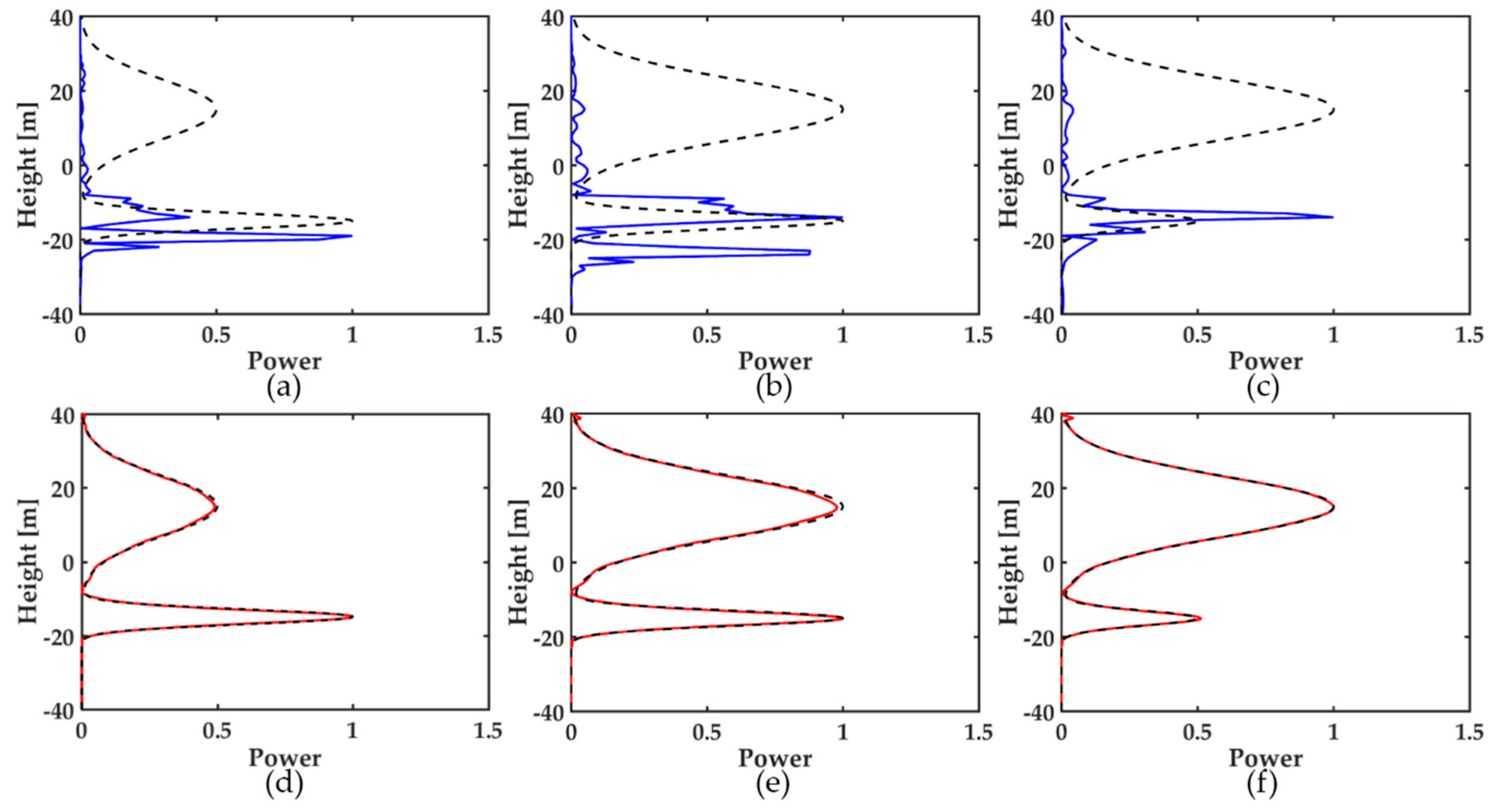
For the three kinds of forest scattering scenarios, wavelet-SPICE fails to reconstruct the vertical structure, while W&O-SPICE successfully obtains the tomogram, as shown in
Figure 2.
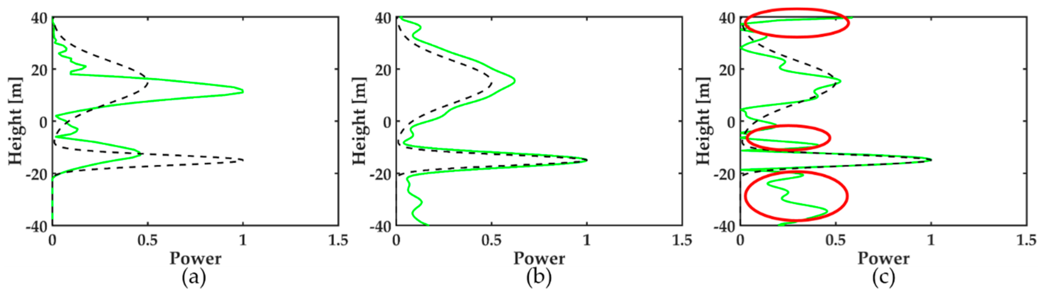
- (2)
For W&O-CS estimator, it is necessary to select the hyperparameter for all the resolution cells. Differences in the selected hyperparameter lead to differences in performance, as shown in
Figure 3. When this hyperparameter is too small, the reconstructed profile will miss the backscattering of targets of interest, even bringing about some misestimations (
Figure 3a). When this hyperparameter is too large, the reconstructed profile will not only reflect the backscattering of targets of interest, but also contains much noise, as shown by the red circles in
Figure 3c. A nice performance can be obtained only through selecting an appropriate hyperparameter (
Figure 3b). Moreover, the hyperparameter is closely related to the noise level of a pixel, and the noise level is different in different pixels. Thus, a selected hyperparameter for a resolution cell may not be suitable for another cell. When the selected hyperparameter can be adaptive to the noise in each pixel, CS can have a nice reconstructed profile.
- (3)
With the reduction of the ground angular spreading, W&O-SPICE shows a good performance in retrieving the vertical structure of the forest, in all cases, and the result is almost the same as the ground truth (see
Figure 4a–c). However, when the ground angular spreading is wide, W&O-CS can reconstruct the vertical structure of the simulated forest signal (
Figure 4d). When the ground angular spreading reduces to moderate, W&O-CS can also detect the ground scattering, but has deviation in the canopy amplitude retrieval. When the ground angular spreading is decreased to narrow, just like the point-like signal, there are deviations in both the canopy and ground amplitude reconstruction.
From the above observations, it can be seen that wavelet-SPICE is not able to obtain correct reconstruction results because the wavelet basis only has good sparseness on the smooth signals, such as the backscattering power of the forest canopy. When the smooth signal is mixed with an approximately point-like signal, such as the ground backscattering power, the sparseness of the wavelet basis is seriously reduced. However, the W&O sparse basis can solve this problem, and it can not only ensure the sparsity of the smooth signal, but it can also keep the sparseness of point-like signals. In addition, the SPICE algorithm adaptively takes into account the noise for every resolution cell, which avoids the need to select a hyperparameter.
4. Real-Data Experiments and Results
In order to further demonstrate the feasibility and effectiveness of W&O-SPICE for a small number of non-uniformly distributed baselines, a real airborne SAR dataset was applied in TomoSAR to obtain the vertical structure of a forest.
4.1. Study Area and Dataset
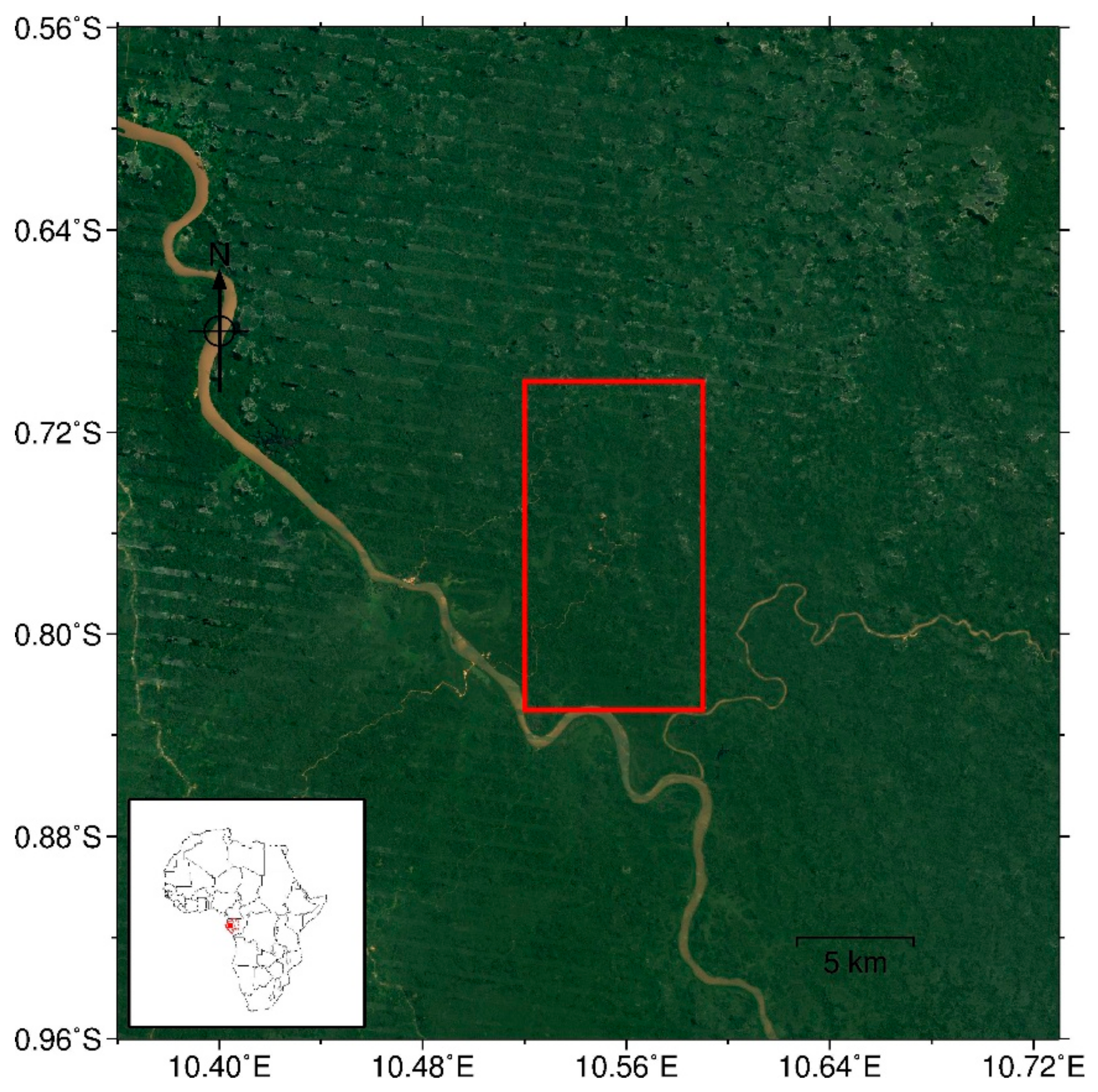
The study area is located at Mabounie (
Figure 5), Gabon, west-central Africa, and is 180 km away from the capital airport. It is known as a mining exploration site and is an important test site for tropical rain forests. There are both mature forests and degraded forests in the area. The weather is hot and humid, and the average annual temperature is about 26 °C. Moreover, the annual rainfall ranges between 1500 mm and 3000 mm. The topography ranges between 0 and 170 m [
36,
37].
Three P-band fully polarimetric SAR images with non-uniformly distributed baselines were obtained over the study area, which had been already preprocessed into tomographic dataset by the German Aerospace Center (DLR). These images were acquired by the F-SAR airborne system in the framework of the AfriSAR campaign, aiming at addressing the planning requirements for the development of the European Space Agency’s (ESA) BIOMASS mission. During the early stage of the BIOMASS feasibility and consolidation study, the vertical structure of the tropical forest had already been reconstructed as part of the TropiSAR 2009 campaign. The objective of TropiSAR 2009 was to study Amazonian forest types characterized by high biomass density (higher than 300 t/ha). However, the tropical forest around the equatorial belt is very different from the Amazonian forest, as their biomass conditions range from 100 t/ha to 300 t/ha [
36]. Thus, it was necessary to develop and verify the BIOMASS mission performance on this kind of tropical forest.
The parameters of the collected data are shown in
Table 2 and
Table 3. The range resolution is 3.84 m and the azimuth resolution is 2.0 m. The Rayleigh resolution along the elevation is 40 m. The incidence angle varies from 25° to 55° [
36].
In order to validate the TomoSAR results, we used the LiDAR data acquired by the LVIS system operated by NASA over this study area in February 2016, in a joint cooperation between the ESA, the DLR, ONERA, the ANPN, NASA, and the University of Maryland. The LVIS system was installed on a NASA Langley B200 plane with a flight height of 7315 m [
36]. The LiDAR footprint was about 20 m wide on the ground. Based on these LiDAR data, the digital terrain model (DTM) and canopy height model (CHM) could be generated.
4.2. Results and Analysis
4.2.1. Tomogram of the Selected Profile
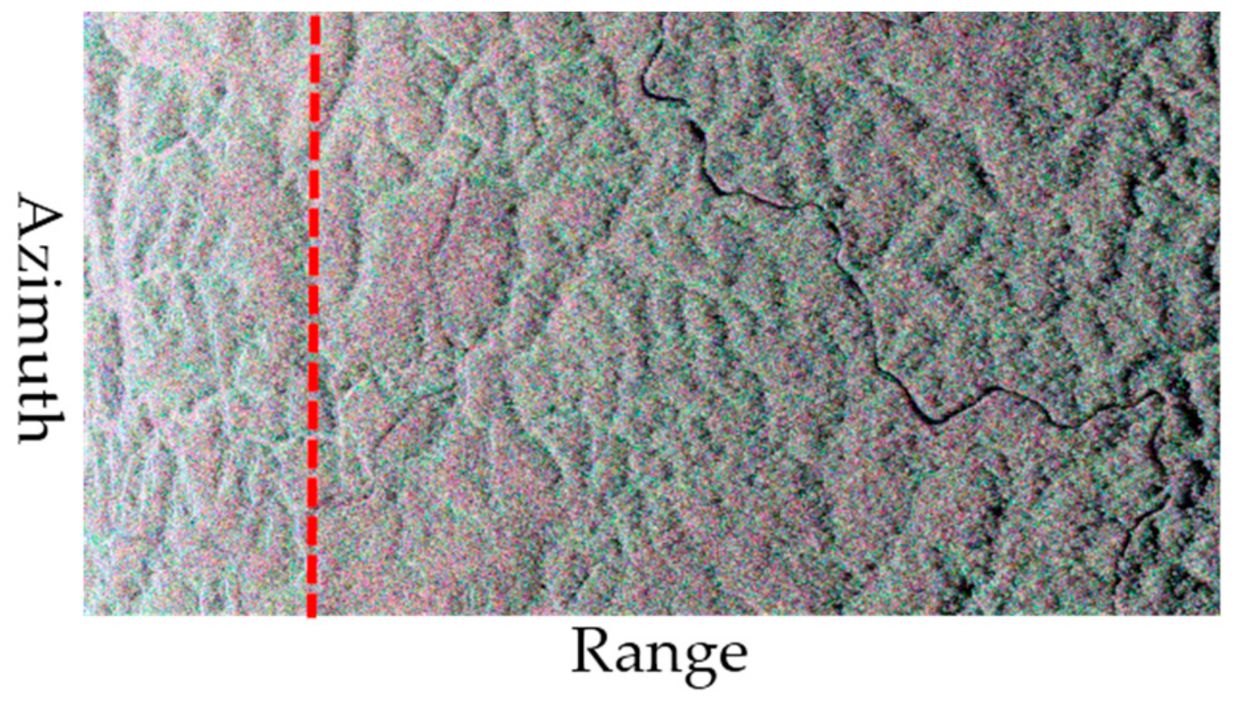
An azimuth profile (at the 200th azimuth resolution cell) was selected to perform tomographic focusing (as shown in
Figure 6). The size of the estimation window applied in the experiments was 31 × 31 pixels (slant range/azimuth), corresponding to about 180 m × 60 m (ground range/azimuth).
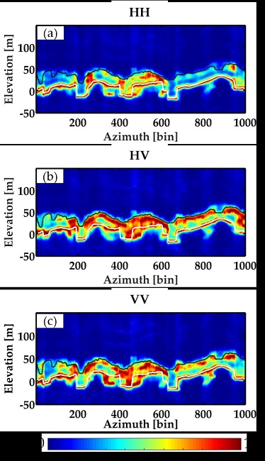
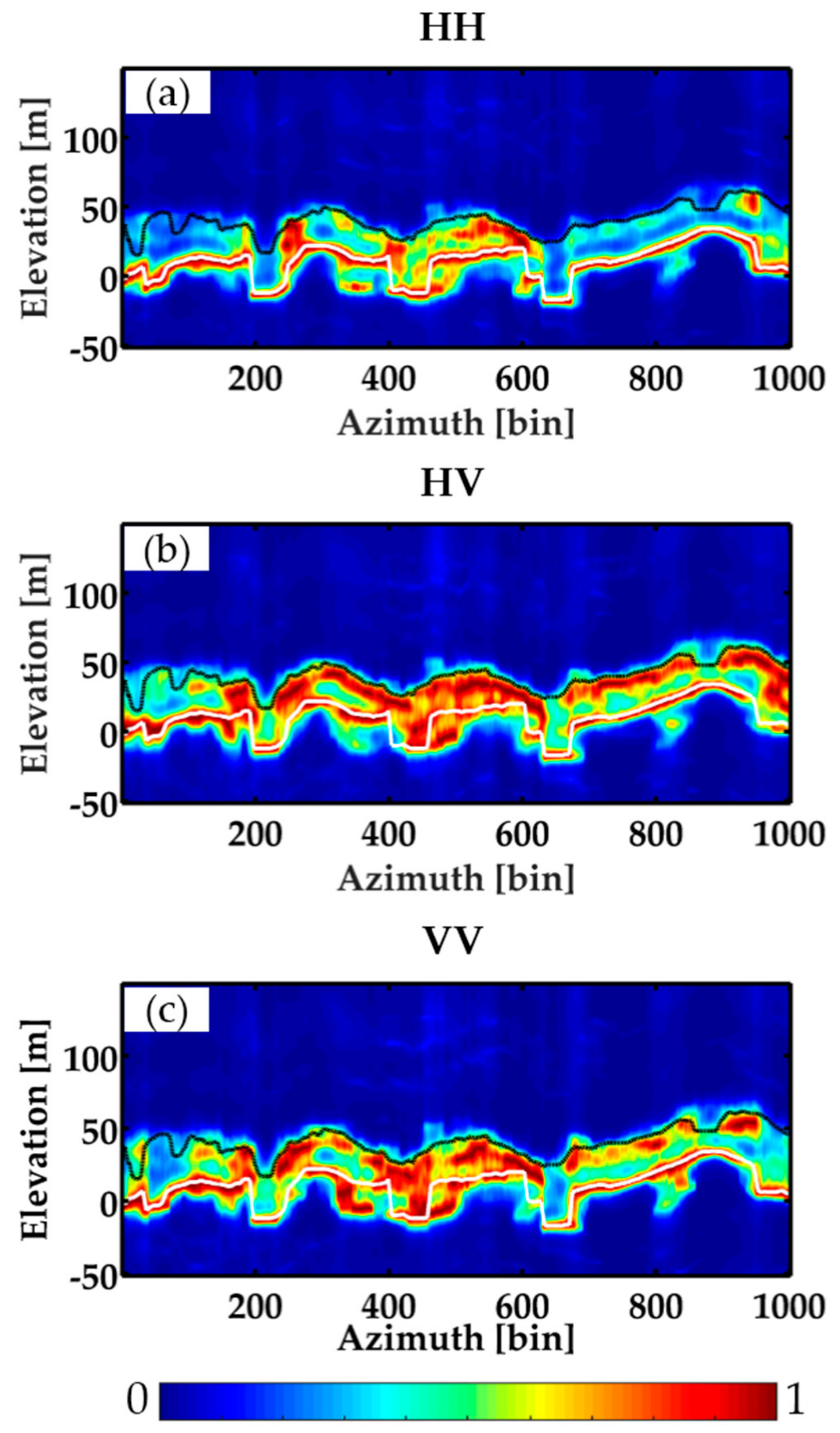
Figure 7 shows tomograms of the selected azimuth profile in the three polarimetric modes. For the sake of a clear contrastive analysis, the LiDAR DTM and CHM were projected into SAR geometric coordinates. A number of observations can be made: (1) The vertical structure of the forest can be reconstructed from each polarimetric dataset. (2) For the HH polarization, the ground backscattering dominates. Moreover, the ground scattering phase centers detected by the W&O-SPICE algorithm show a good consistency with the LiDAR DTM. (3) For the HV polarization, the dominant scattering is the canopy backscattering, and the corresponding detected phase centers have a similar wave trend to the LiDAR CHM. (4) For the VV polarization, the W&O-SPICE algorithm detects some ground scattering phase centers and some canopy scattering phase centers.
The above observations indicate that the backscattering power for the HH polarimetric channel and HV polarimetric channel mainly comes from the ground and forest canopy, respectively. Thus, the underlying topography can be estimated from the results in the HH polarization, and the forest canopy height can be obtained from the results of the HV polarimetric channel.
4.2.2. Underlying Topography Estimation
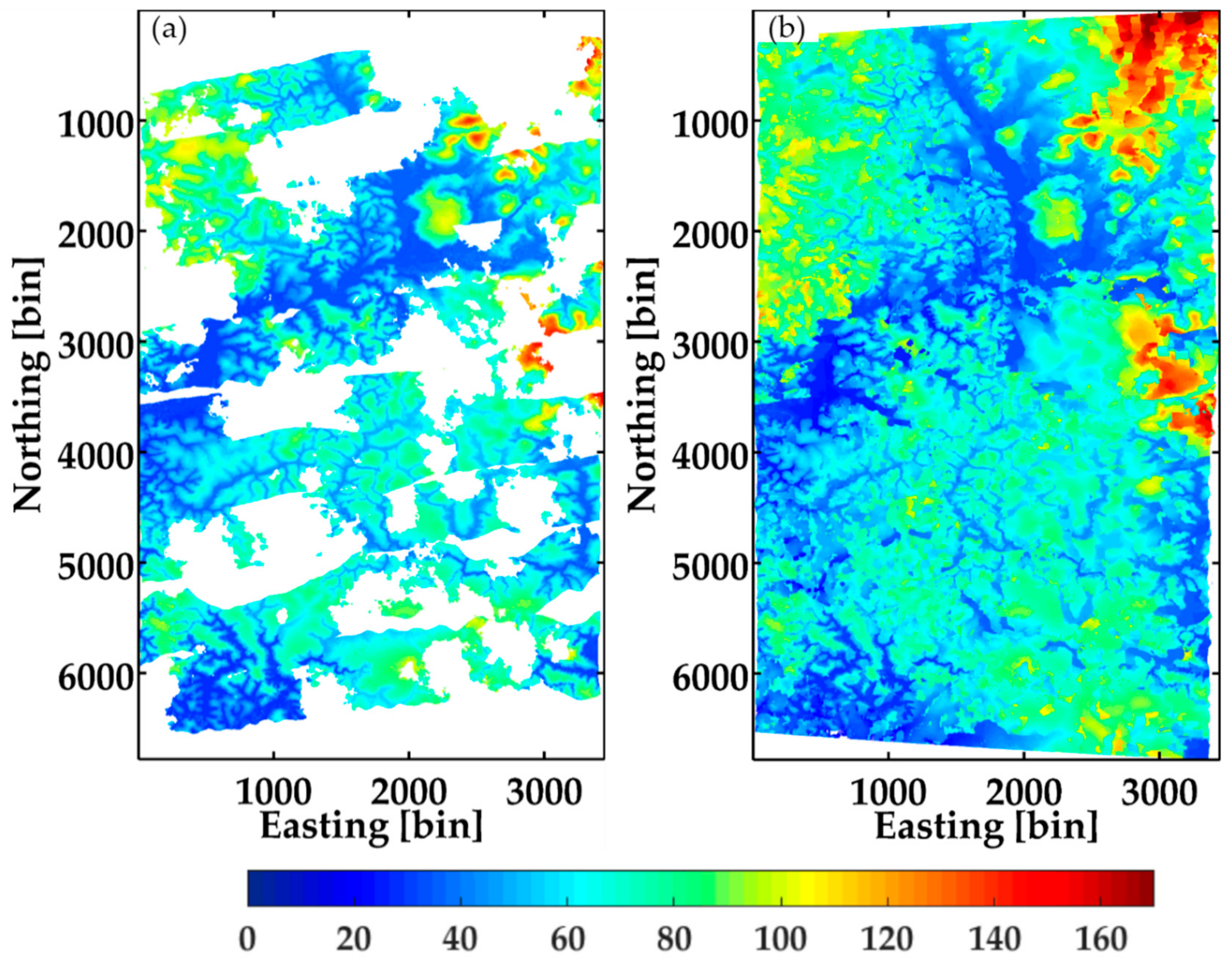
For one pixel, the first two strongest peaks generally reflect the ground scattering and forest canopy scattering. The heights of these two peaks are respectively the ground height and the forest canopy scattering phase height. Thus, the smaller value between two heights is the ground height. By detecting all the ground peaks of the tomograms in the HH polarimetric channel, the underlying topography was estimated using the W&O-SPICE algorithm, as shown in
Figure 8. In order to compare this with the LiDAR DTM, the estimated underlying topography was projected into the geographic coordinate system. Due to the influence of cloud and fog, there are many cavities in the LiDAR DTM, as shown in
Figure 8a. The underlying topography estimated by the W&O-SPICE TomoSAR method ranges between 0 and 170 m, which corresponds with the ground truth. Moreover, most of the underlying topography estimated by the W&O-SPICE TomoSAR method is consistent with the LiDAR DTM, especially in the details.
In addition, to evaluate the performance of the W&O-SPICE TomoSAR method, we calculated the mean and the root-mean-square error (RMSE) of the estimated underlying topography with respect to the LiDAR DTM, and the two values are, respectively, 1.05 m and 6.40 m (see
Table 4).
4.2.3. Forest Height Estimation
Based on the analysis given in
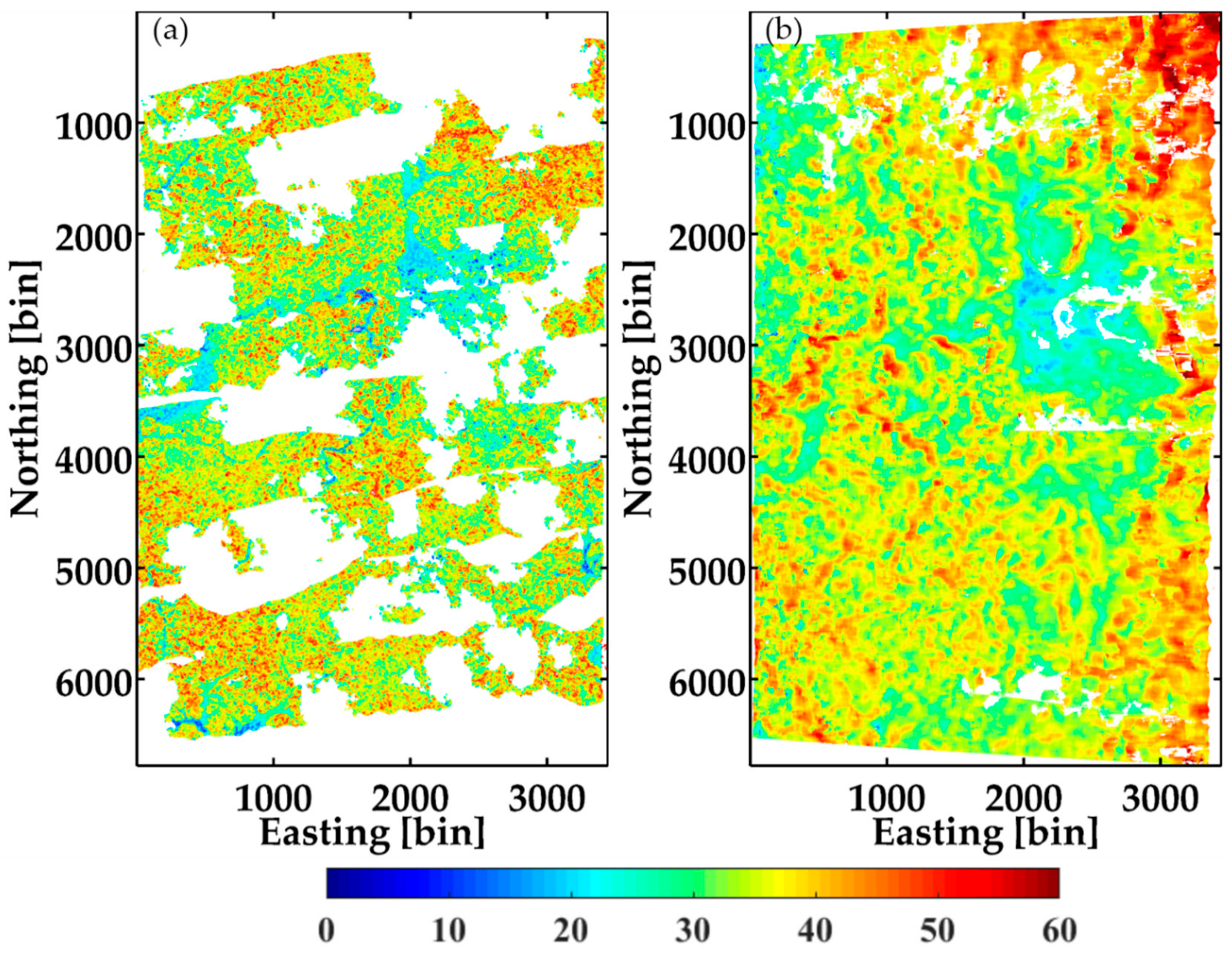
Section 4.2.1, the canopy height was estimated with the results of the HV polarimetric channel. The forest height could then be obtained as the difference between the canopy height and the ground height, as shown in
Figure 9. The detailed process of canopy height estimation can be referred in References [
10,
11,
12,
28]. Since only three images were applied in the tomographic focusing, it was impossible to provide a correct estimation in some parts (the holes in
Figure 9b). However, the estimated forest height is largely similar to the LiDAR CHM. Moreover, the mean and RMSE of the forest height estimation were also calculated with respect to the LiDAR CHM, and the values are, respectively, 0.02 m and 4.50 m (listed in
Table 5).
The above analysis suggests that the W&O-SPICE algorithm can be used to reconstruct the vertical structure of a forest using only a small number of non-uniformly distributed acquisitions. Although the estimation accuracy of the underlying topography and forest height is not particularly high, it does demonstrate that the W&O-SPICE estimator is a good candidate to estimate the underlying topography and forest height in the case of a small number of polarimetric SAR images with non-uniformly distributed baselines.
5. Discussion
To further verify the performance of the SPICE algorithm based on the W&O sparse basis, the tomographic estimators of CS and the nonparametric spectral estimation methods (beamforming, Capon, and the iterative adaptive approach (IAA)) were also applied in tomographic focusing of the same azimuth profile.
5.1. Comparison between W&O-CS and W&O-SPICE
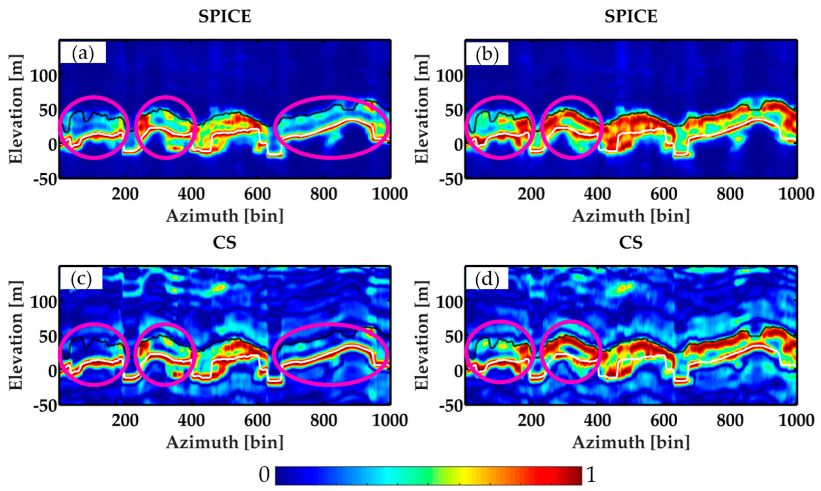
Figure 10 shows tomograms in the HH and HV polarizations estimated by CS based on the W&O sparse basis. It is found that the backscattering power along the vertical direction from W&O-CS is also related to the polarimetric mode: the results in the HH polarization are suitable to recognize the ground scattering, and those in the HV polarization indicate the forest canopy scattering. However, W&O-CS shows a degraded performance in reconstructing the canopy information, especially the parts marked by the purple circles in
Figure 10. This is because the CS algorithm requires the user to select a hyperparameter. If this parameter is too small, it will lead to overfitting, missing some useful information. If this parameter is too large, it will result in underfitting, estimating some unnecessary information besides the parameters of interest. In addition, the selected hyperparameter makes it difficult for CS to adapt to the noise in each resolution cell. Thus, the tomogram estimated by the W&O-CS estimator is clear in some pixels, while it is seriously affected by noise in other pixels. This reduces the accuracy of the underlying topography and forest height estimation.
However, SPICE does not depend on a hyperparameter, and considers the noise of each resolution cell adaptively. Accordingly, the tomograms estimated by W&O-SPICE are almost unaffected by noise. This analysis confirms that SPICE is more suitable for application over forest areas than CS.
5.2. Comparison between the Nonparametric Spectral Estimation Methods and W&O-SPICE
Since nonparametric spectral estimation does not require any prior information, it has been widely used in TomoSAR application over forest areas. Accordingly, the commonly used nonparametric spectral estimators of beamforming, Capon, and IAA [
16,
38] were applied for the tomographic focusing of the selected azimuth profile in the HH and HV polarizations, as shown in
Figure 11. Among the results of these tomographic estimators, beamforming shows the most serious noise in the tomograms. It also fails to separate the ground scattering contribution and the canopy scattering contribution. As for Capon, the noise is much less than for beamforming, but it only detects one scattering phase center in each resolution cell. This means that Capon also cannot separate the ground scattering contribution and the canopy scattering contribution. The reason for this is that both beamforming and Capon follow Shannon’s sampling theorem, and they have a low resolution and serious sidelobes in the case of a small number of acquisitions with non-uniformly distributed baselines. In addition, it can be clearly seen in
Figure 11g,h that IAA can distinguish a few ground scattering phase centers and forest canopy scattering phase centers. However, most of the scattering phase centers are still indistinguishable. Moreover, sidelobes exist in the tomograms estimated by IAA. Therefore, these three estimators cannot be used to obtain the underlying topography and forest height in this case study. However, W&O-SPICE can successfully distinguish the ground and forest canopy scattering contributions, and it successfully estimated the underlying topography and forest height over this study area.
The above observations suggests that SPICE has a higher resolution than beamforming, Capon, and IAA in the case of a small number of non-uniformly distributed acquisitions, which is consistent with the findings in References [
32,
33,
34].
From the above analysis, it is found that it makes it possible for TomoSAR to reconstruct the forest vertical structure with a small number of non-uniformly distributed acquisitions. This provides an opportunity for the extraction of underlying topography and forest height in a large scale. Moreover, our future works will also focus on analyzing the feasibility and effectiveness of the proposed approach for polarimetric TomoSAR over forest areas.
6. Conclusions
In this paper, we have proposed the W&O-SPICE TomoSAR method for use with a small number of acquisitions with non-uniformly distributed baselines. The W&O sparse basis is made up of the wavelet basis and orthogonal basis, which can not only ensure the sparsity of the forest backscattering power, but can also keep the sparseness of the ground backscattering power. SPICE, as a sparse spectral estimation technique, can obtain a high vertical resolution, even with a small number of acquisitions with non-uniformly distributed baselines. Moreover, it does not require the user to select a hyperparameter.
Through several sets of simulation experiments, we found that SPICE based on the W&O sparse basis can reconstruct the vertical structure of forest in three kinds of ground-to-canopy scattering power ratios. However, SPICE based on the wavelet basis cannot achieve this. Moreover, W&O-SPICE can still obtain a good reconstruction performance as the ground angular spread becomes narrower and narrower.
Three P-band fully polarimetric airborne SAR images with non-uniformly distributed baselines were applied in tomographic focusing, to demonstrate the feasibility and effectiveness of the proposed method. The results showed that the W&O-SPICE algorithm could successfully reconstruct the vertical structure of the tropical forest in Mabounie, Gabon, for the three polarimetric channels. Based on the results in the HH polarization and HV polarization, both the underlying topography and the forest height were estimated. With respect to the LiDAR DTM and CHM, the estimated RMSEs were 6.40 m and 4.50 m for the underlying topography and forest height, respectively. Furthermore, the TomoSAR methods of W&O-CS, beamforming, Capon, and IAA were also used to obtain tomograms for the selected azimuth profile. Compared to W&O-SPICE, W&O-CS could also recognize the ground and forest canopy scattering phase centers, but it was greatly affected by noise. This is because CS depends on the selected hyperparameter. As for beamforming and Capon, they were both unable to separate the ground scattering contribution and the forest canopy scattering contribution. Although IAA could distinguish a few ground scattering centers and forest canopy scattering centers, it failed to separate most of them.
In conclusion, the W&O-SPICE estimator showed advantages over the TomoSAR estimators of CS, beamforming, Capon, and IAA in this case study. In the case of a small number of non-uniformly distributed acquisitions, W&O-SPICE is better able to reconstruct the vertical structure of forest and estimate the underlying topography and forest height.
Author Contributions
X.P. conceived the idea, designed and performed the experiments, produced the results, and drafted the manuscript. X.L. and J.Z. contributed to the discussion of the idea and the results. C.W. acquired the datasets. L.L., Y.D., H.F., Z.Y., and Q.X. contributed to the discussion of the results and the revision of the article. All authors reviewed and approved the manuscript.
Funding
This research was funded by the National Natural Science Foundation of China (No. 41571360, No. 41531068, No. 41820104005, No. 41842059, No. 41804003) and China Postdoctoral Science Foundation (No. 2016M601110). The airborne F-SAR datasets were provided by the ESA (No. 38329).
Conflicts of Interest
The authors declare no conflict of interest.
References
- Houghton, R.A.; Hall, F.; Goetz, S.J. Importance of Biomass in the Global Carbon Cycle. J. Geophys. Res. 2009, 114, 1–13. [Google Scholar] [CrossRef]
- Toan, T.L.; Quegan, S.; Davidson, M.W.J.; Balzter, H.; Paillou, P.; Papathanassiou, K.; Plummer, S.; Rocca, F.; Saatchi, S.; Shugart, H.; et al. The BIOMASS Mission: Mapping Global Forest Biomass to Better Understand the Terrestrial Carbon Cycle. Remote Sens. Environ. 2011, 115, 2850–2860. [Google Scholar] [CrossRef]
- Hall, F.G.; Bergen, K.; Blair, J.B.; Dubayah, R.; Houghton, R.; Hurtt, G.; Kellndorfer, J.; Lefsky, M.; Ranson, J.; Saatchi, S.; et al. Characterizing 3D Vegetation Structure from Space: Mission Requirements. Remote Sens. Environ. 2011, 115, 2753–2775. [Google Scholar] [CrossRef]
- Kumar, S.; Khati, U.G.; Chandola, S.; Agrawal, S.; Kushwaha, S.P.S. Polarimetric SAR Interferometry based Modeling for Tree Height and Aboveground Biomass Retrieval in a Tropical Deciduous Forest. Adv. Space Res. 2017, 60, 571–586. [Google Scholar] [CrossRef]
- Frey, O.; Morsdorf, F.; Meier, E. Tomographic imaging of a forested area by airborne multi-baseline P-band SAR. Sensors 2008, 8, 5884–5896. [Google Scholar] [CrossRef] [PubMed]
- Frey, O.; Meier, E. Analyzing Tomographic SAR Data of a Forest with Respect to Frequency, Polarization, and Focusing Technique. IEEE Trans. Geosci. Remote Sens. 2011, 49, 3648–3659. [Google Scholar] [CrossRef]
- Reigber, A.; Moreira, A. First Demonstration of Airborne SAR Tomography Using Multibaseline L-Band Data. IEEE Trans. Geosci. Remote Sens. 2000, 38, 2142–2152. [Google Scholar] [CrossRef]
- Reigber, A.; Papathanassiou, K.; Cloude, S.; Moreira, A. SAR Tomography and Interferometry for the Remote Sensing of Forested Terrain. Eur. Synth. Apert. Radar Conf. 2000, 55, 119–122. [Google Scholar] [CrossRef]
- Lombardini, F.; Reigber, A. Adaptive spectral estimation for multibaseline SAR tomography with airborne L-band data. In Proceedings of the 2003 IEEE International Geoscience and Remote Sensing Symposium (IGARSS), Toulouse, France, 21–25 July 2003; pp. 2014–2016. [Google Scholar]
- Tebaldini, S. Algebraic Synthesis of Forest Scenarios from Multibaseline PolInSAR Data. IEEE Trans. Geosci. Remote Sens. 2009, 47, 4132–4142. [Google Scholar] [CrossRef]
- Minh, D.H.T.; Toan, T.L.; Rocca, F.; Tebaldini, S.; Villard, L.; Réjou-Méchain, M.; Phillips, O.; Feldpausch, T.R.; Dubois-Fernandez, P.; Scipal, K.; et al. SAR Tomography for the Retrieval of Forest Biomass and Height: Cross-Validation at Two Tropical Forest Sites in French Guiana. Remote Sens. Environ. 2016, 175, 138–147. [Google Scholar] [CrossRef]
- Tebaldini, S.; Rocca, F. Multibaseline Polarimetric SAR Tomography of a Boreal Forest at P-And L-Bands. IEEE Trans. Geosci. Remote Sens. 2012, 50, 232–246. [Google Scholar] [CrossRef]
- Pardini, M.; Papathanassiou, K. On the Estimation of Ground and Volume Polarimetric Covariances in Forest Scenarios with SAR Tomography. IEEE Geosci. Remote Sens. Lett. 2017, 14, 1860–1864. [Google Scholar] [CrossRef]
- Kumar, S.; Joshi, S.K.; Govil, H. Spaceborne PolSAR Tomography for Forest Height Retrieval. IEEE J. Sel. Top. Appl. Earth Obs. Remote Sens. 2017, 10, 5175–5185. [Google Scholar] [CrossRef]
- Gustavo, D.; del Campo, M.; Shkvarko, Y.V.; Reigber, A.; Nannini, M. TomoSAR imaging for the study of forested areas: A virtual adaptive Beamforming approach. Remote Sens. 2018, 10, 1822. [Google Scholar]
- Peng, X.; Wang, C.; Li, X.; Du, Y.; Fu, H.; Yang, Z.; Xie, Q. Three-dimensional structure inversion of buildings with nonparametric iterative adaptive approach using SAR tomography. Remote Sens. 2018, 10, 1004. [Google Scholar] [CrossRef]
- Huang, Y.; Ferro-Famil, L.; Lardeux, C. Polarimetric SAR tomography of tropical forests at P-band. In Proceedings of the 2011 IEEE International Geoscience and Remote Sensing Symposium (IGARSS), Vancouver, BC, Canada, 24–29 July 2011; pp. 1373–1376. [Google Scholar]
- Huang, Y.; Ferro-Famil, L.; Reigber, A. Under-foliage Object imaging using SAR tomography and polarimetric spectral estimators. IEEE Trans. Geosci. Remote Sens. 2012, 50, 2213–2225. [Google Scholar] [CrossRef]
- Meglio, F.; Panariello, G.; Schirinzi, G. Three dimensional SAR image focusing from non-uniform samples. In Proceedings of the 2007 IEEE International Geoscience and Remote Sensing Symposium, Barcelona, Spain, 23–27 July 2007; pp. 528–531. [Google Scholar]
- Lombardini, F.; Pardini, M.; Gini, F. Sector Interpolation for 3D SAR imaging with baseline diversity data. In Proceedings of the International Waveform Diversity and Design Conference (WDD), Pisa, Italy, 4–8 June 2007; pp. 297–301. [Google Scholar]
- Lombardini, F.; Pardini, M. 3-D SAR Tomography: The multibaseline sector interpolation approach. IEEE Geosci. Remote Sens. Lett. 2008, 5, 630–634. [Google Scholar] [CrossRef]
- Aguilera, E.; Nannini, M.; Reigber, A. Wavelet-based compressed sensing for SAR tomography of forested areas. IEEE Trans. Geosci. Remote Sens. 2013, 51, 5283–5295. [Google Scholar] [CrossRef]
- Liang, L.; Li, X.; Gao, X.; Guo, H. Multibaseline polarimetric synthetic aperture radar tomography of forested areas using wavelet-based distribution compressive sensing. J. Appl. Remote Sens. 2015, 9. [Google Scholar] [CrossRef]
- Zhu, X.; Bamler, R. Tomographic SAR inversion by L-1-Norm regularization-the compressive sensing approach. IEEE Trans. Geosci. Remote Sens. 2010, 48, 3839–3846. [Google Scholar] [CrossRef]
- Budillon, A.; Evangelista, A.; Schirinzi, G. Three dimensional SAR focusing from multi-pass signals using compressive sampling. IEEE Trans. Geosci. Remote Sens. 2011, 49, 488–499. [Google Scholar] [CrossRef]
- Zhu, X.; Bamler, R. Super-resolution power and robustness of compressive sensing for spectral estimation with application to spaceborne tomographic SAR. IEEE Trans. Geosci. Remote Sens. 2012, 50, 247–258. [Google Scholar] [CrossRef]
- Lei, L.; Huadong, G.; Li, X. Three-Dimensional structural parameter inversion of buildings by distributed compressive sensing-based polarimetric SAR tomography using a small number of baselines. IEEE J. Sel. Top. Appl. Earth Observ. Remote Sens. 2014, 3, 4218–4230. [Google Scholar]
- Li, X.; Liang, L.; Guo, H. Compressive sensing for multibaseline polarimetric SAR tomography of forested areas. IEEE Trans. Geosci. Remote Sens. 2016, 54, 153–166. [Google Scholar] [CrossRef]
- Cazcarra-Bes, V.; Tello-Alonso, M.; Fischer, R.; Heym, M.; Papathanassiou, K. Monitoring of forest structure dynamics by means of L-band SAR tomography. Remote Sens. 2017, 9, 1229. [Google Scholar] [CrossRef]
- Huang, Y.; Levy-Vehel, J.; Ferro-Famil, L.; Reigber, A. Three-dimensional imaging of objects concealed below a forest canopy using SAR tomography at L-band and wavelet-based sparse estimation. IEEE Geosci. Remote Sens. Lett. 2017, 14, 1454–1458. [Google Scholar] [CrossRef]
- Liang, L.; Li, X.; Ferro-Famil, L.; Guo, H.; Zhang, L.; Wu, W. Urban area tomography using a sparse representation based two-dimensional spectral analysis technique. Remote Sens. 2018, 10, 109. [Google Scholar] [CrossRef]
- Stocia, P.; Babu, P.; Li, J. SPICE: A sparse covariance-based estimation method for array processing. IEEE Trans. Signal Process. 2011, 59, 629–638. [Google Scholar]
- Stocia, P.; Babu, P.; Li, J. New method of sparse parameter estimation in separable models and its use for spectral analysis of irregularly sampled data. IEEE Trans. Signal Process. 2011, 59, 35–47. [Google Scholar]
- Stoica, P.; Babu, P. SPICE and LIKES: Two hyperparameter-free methods for sparse-parameter estimation. Signal Process. 2012, 92, 1580–1590. [Google Scholar] [CrossRef]
- Peng, X.; Li, X.; Wang, C.; Fu, H.; Du, Y. A maximum likelihood based nonparametric iterative adaptive method of synthetic aperture radar tomography and its application for estimating underlying topography and forest height. Sensors 2018, 18, 2459. [Google Scholar] [CrossRef] [PubMed]
- European Space Agency. Technical Assistance for the Development of Airborne SAR and Geophysical Measurements during the AfriSAR Experiment; Final Report; European Space Agency: Paris, France, April 2017. [Google Scholar]
- Pardini, M.; Tello, M.; Cazcarra-Bes, V.; Papathanassiou, K.P. L- and P-Band 3-D SAR reflectivity profiles versus Lidar waveforms: The AfriSAR case. IEEE J. Sel. Top. Appl. Earth Observ. Remote Sens. 2018, 11, 4218–4230. [Google Scholar] [CrossRef]
- Del Campo, G.D.M.; Reigber, A.; Shkvarko, Y.V. Resolution enhanced SAR tomography: A Nonparametric Iterative Adaptive Approach. In Proceedings of the International Geoscience and Remote Sensing Symposium (IGARSS), Beijing, China, 10–15 July 2016; pp. 3238–3241. [Google Scholar]
Figure 1.
The sparse transformation of backscattering power over forest areas.
Figure 1.
The sparse transformation of backscattering power over forest areas.
Figure 2.
The reconstructed reflectivity profiles by the wavelet-sparse iterative covariance-based estimation (SPICE) and wavelet and orthogonal sparse basis (W&O-SPICE) synthetic aperture radar tomography (TomoSAR) methods for a simulated signal with different ground-to-canopy power ratios: (a) wavelet-SPICE for r > 1; (b) wavelet-SPICE for r = 1; (c) wavelet-SPICE for r < 1; (d) W&O-SPICE for r > 1; (e) W&O-SPICE for r = 1; (f) W&O-SPICE for r < 1. The black dotted lines are the normalized simulated profiles. The blue solid lines are the reconstructed reflectivity profiles of wavelet-SPICE. The red solid lines are the reconstructed reflectivity profiles of W&O-SPICE.
Figure 3.
The reconstructed reflectivity profiles by the W&O-compressive sensing (CS) TomoSAR method for a simulated signal (r > 1) with different hyperparameters: (a) 100; (b) 1000; (c) 10,000.
Figure 3.
The reconstructed reflectivity profiles by the W&O-compressive sensing (CS) TomoSAR method for a simulated signal (r > 1) with different hyperparameters: (a) 100; (b) 1000; (c) 10,000.
Figure 4.
The reconstructed reflectivity profiles by the W&O-CS and W&O-SPICE TomoSAR methods for a simulated signal with different ground angular spreading values with the same forest scattering scenario (r > 1): (a) W&O-CS for the wide ground angular spreading; (b) W&O-CS for the moderate ground angular spreading; (c) W&O-CS for the narrow ground angular spreading; (d) W&O-SPICE for the wide ground angular spreading; (e) W&O-SPICE for the moderate ground angular spreading; (f) W&O-SPICE for the narrow ground angular spreading. The black dotted lines are the normalized simulated profiles. The blue solid lines are the reconstructed reflectivity profiles of wavelet-SPICE. The red solid lines are the reconstructed reflectivity profiles of W&O-SPICE.
Figure 5.
Geographic location of the study area marked in an optical image. The red rectangle represents the footprint of the dataset.
Figure 5.
Geographic location of the study area marked in an optical image. The red rectangle represents the footprint of the dataset.
Figure 6.
The selected azimuth profile (red dotted line) in the Pauli SAR image.
Figure 6.
The selected azimuth profile (red dotted line) in the Pauli SAR image.
Figure 7.
Tomograms estimated by the W&O-SPICE algorithm in the three polarimetric channels: (a) HH; (b) HV; (c) VV. The black solid line represents the LiDAR canopy height model (CHM) and the white solid line represents the LiDAR digital terrain model (DTM).
Figure 7.
Tomograms estimated by the W&O-SPICE algorithm in the three polarimetric channels: (a) HH; (b) HV; (c) VV. The black solid line represents the LiDAR canopy height model (CHM) and the white solid line represents the LiDAR digital terrain model (DTM).
Figure 8.
(a) The LiDAR DTM. (b) The underlying topography estimated by the W&O-SPICE TomoSAR method.
Figure 8.
(a) The LiDAR DTM. (b) The underlying topography estimated by the W&O-SPICE TomoSAR method.
Figure 9.
(a) The LiDAR CHM. (b) The forest height estimated by the W&O-SPICE TomoSAR method.
Figure 9.
(a) The LiDAR CHM. (b) The forest height estimated by the W&O-SPICE TomoSAR method.
Figure 10.
Tomograms estimated by the two tomographic algorithms in two polarimetric channels: (a) W&O-SPICE in the HH polarization; (b) W&O-SPICE in the HV polarization; (c) W&O-CS in the HH polarization; (d) W&O-CS in the HV polarization. The solid black line represents the LiDAR CHM, and the solid white line represents the LiDAR DTM.
Figure 11.
Tomograms estimated by the three tomographic algorithms in two polarimetric channels: (a) W&O-SPICE in the HH polarization; (b) W&O-SPICE in the HV polarization; (c) beamforming in the HH polarization; (d) beamforming in the HV polarization; (e) Capon in the HH polarization; (f) Capon in the HV polarization; (g) IAA in the HH polarization; (h) IAA in the HV polarization. The solid black line represents the LiDAR CHM, and the solid white line represents the LiDAR DTM.
Table 1.
Pseudocode of the W&O-SPICE algorithm.
Table 1.
Pseudocode of the W&O-SPICE algorithm.
| Initialization |
|---|
| … |
|
| Iteration |
| repeat |
- 1.
|
- 2.
|
- 3.
|
- 4.
|
| Until (convergence) |
Table 2.
Parameters of the F-SAR airborne system.
Table 2.
Parameters of the F-SAR airborne system.
| Polarization | Wavelength | Incidence Angle | Slant Range | Azimuth Resolution | Range Resolution |
|---|
| HH + HV + VV | 0.6897 m | 25–55° | 6096 m | 3.84 m | 2.0 m |
Table 3.
The baseline information for the InSAR pairs.
Table 3.
The baseline information for the InSAR pairs.
| Identifier | Acquisition Date | Baseline (m) |
|---|
| 07-02 | 11/02/2016 | 0 |
| 07-05 | 10 |
| 07-15 | 60 |
Table 4.
The mean and RMSE of the underlying topography estimated by the W&O-SPICE TomoSAR method with respect to the LiDAR DTM.
Table 4.
The mean and RMSE of the underlying topography estimated by the W&O-SPICE TomoSAR method with respect to the LiDAR DTM.
| TomoSAR w.r.t LiDAR | Mean | RMSE |
|---|
| DTM (m) | 1.05 | 6.40 |
Table 5.
The mean and RMSE of the forest height estimated by the W&O-SPICE TomoSAR method with respect to the LiDAR CHM.
Table 5.
The mean and RMSE of the forest height estimated by the W&O-SPICE TomoSAR method with respect to the LiDAR CHM.
| TomoSAR w.r.t LiDAR | Mean | RMSE |
|---|
| Forest height (m) | 0.02 | 4.50 |
© 2019 by the authors. Licensee MDPI, Basel, Switzerland. This article is an open access article distributed under the terms and conditions of the Creative Commons Attribution (CC BY) license (http://creativecommons.org/licenses/by/4.0/).

 ,
, 


