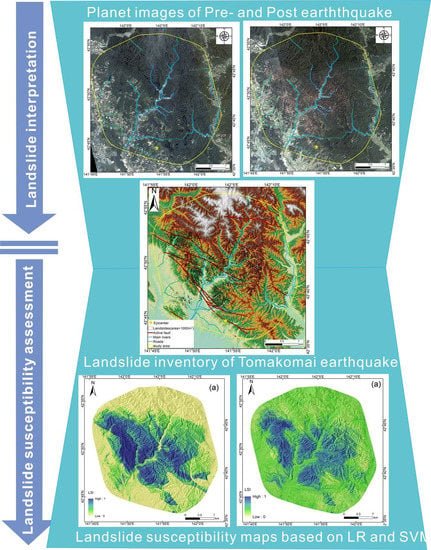
Planet Image-Based Inventorying and Machine Learning-Based Susceptibility Mapping for the Landslides Triggered by the 2018 Mw6.6 Tomakomai, Japan Earthquake


Abstract
:
1. Introduction
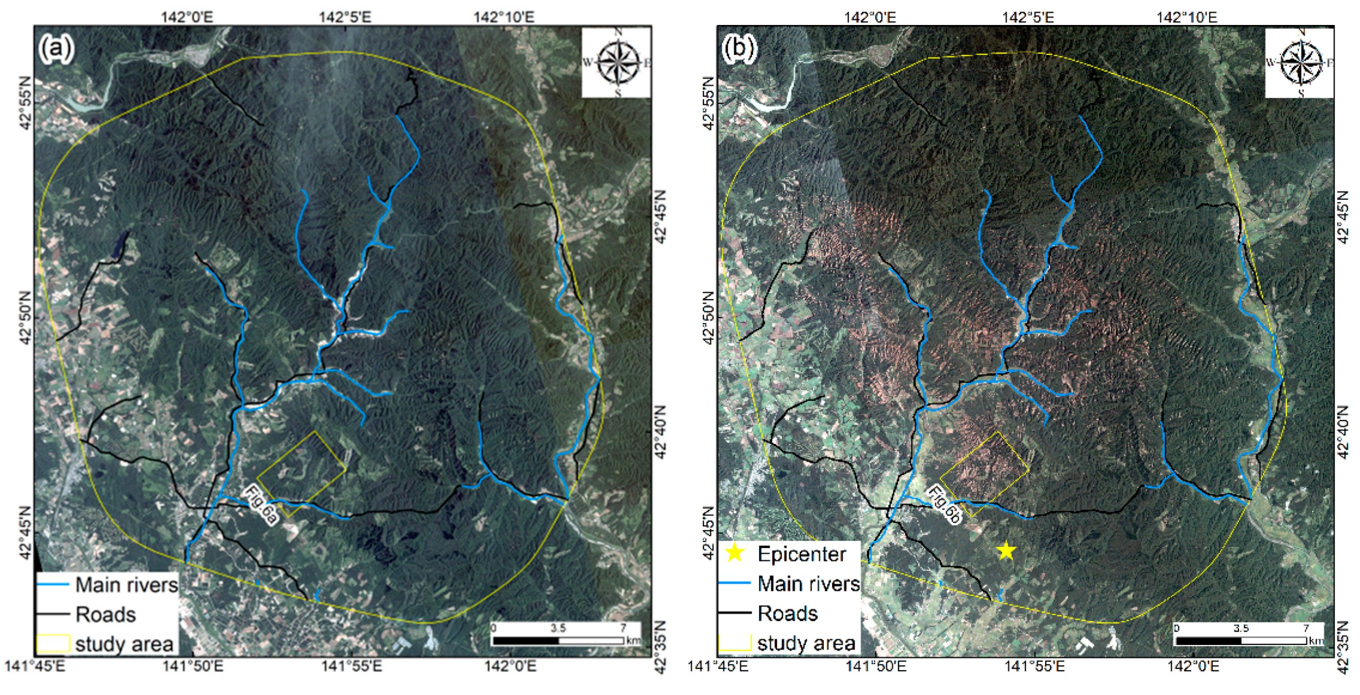
2. Study Area
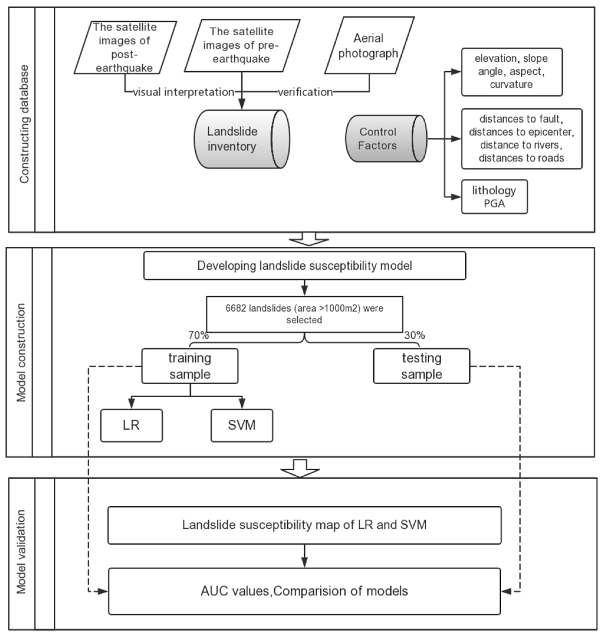
3. Data and Method
3.1. Data Source
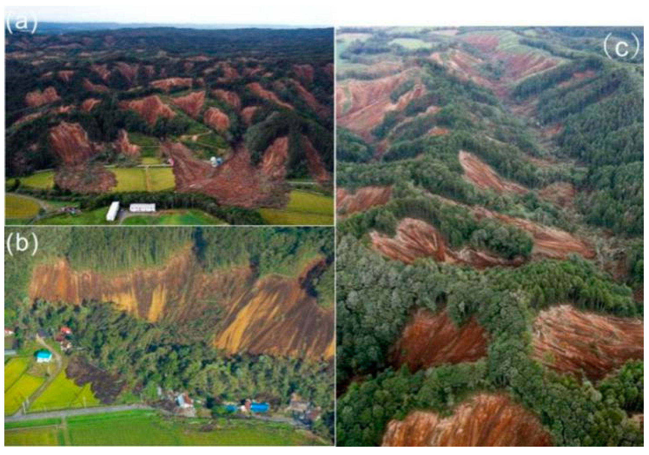
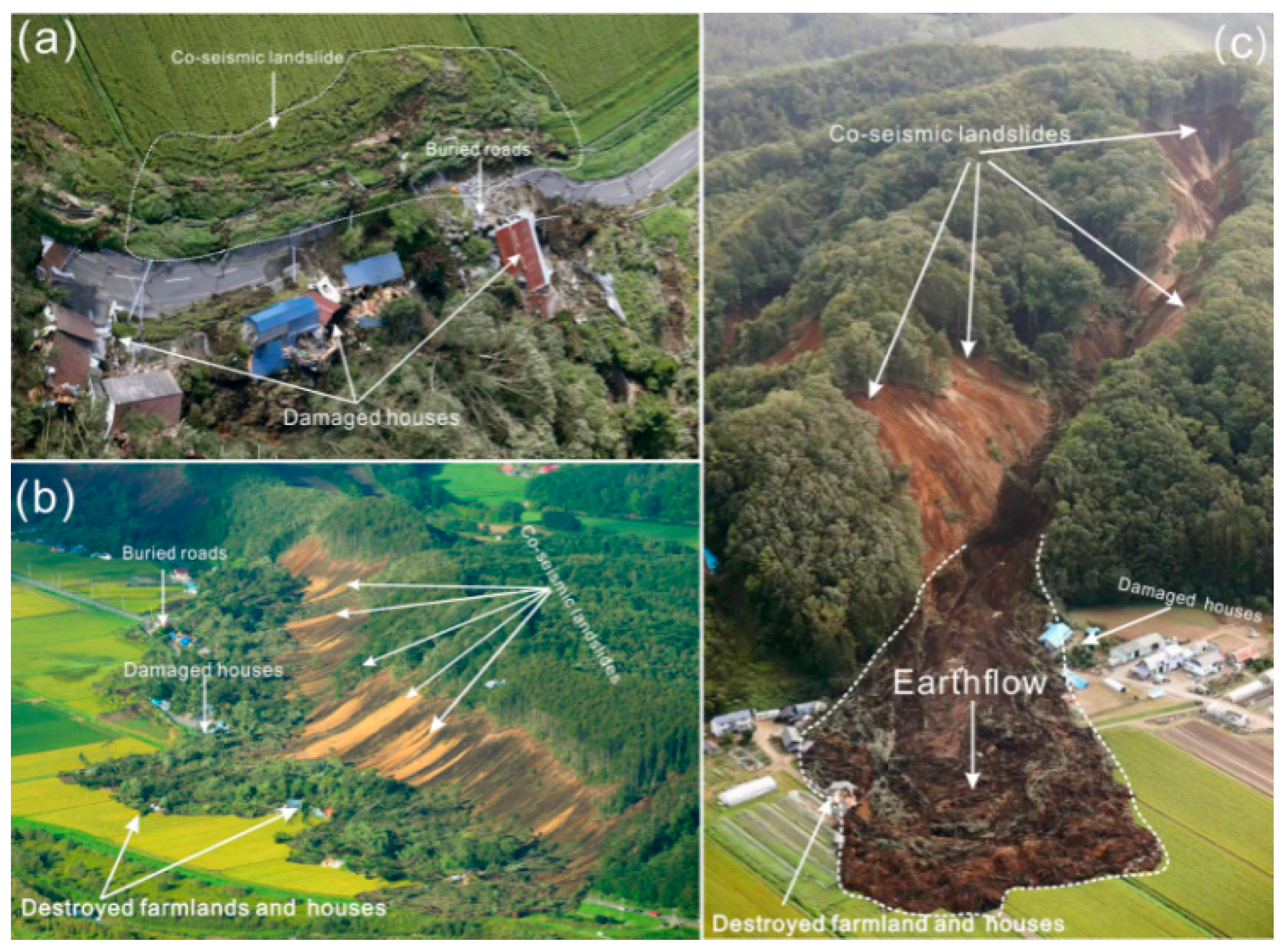
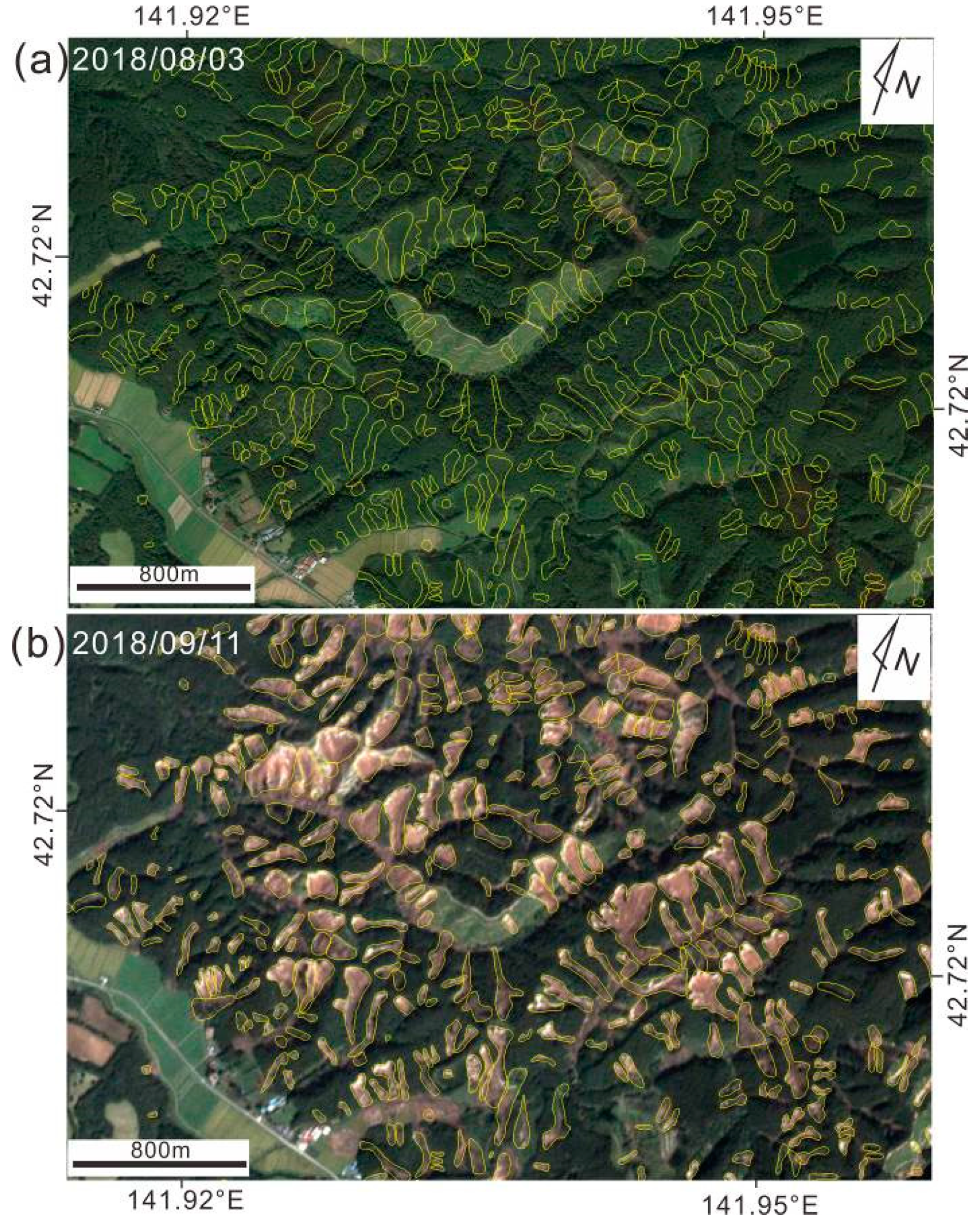
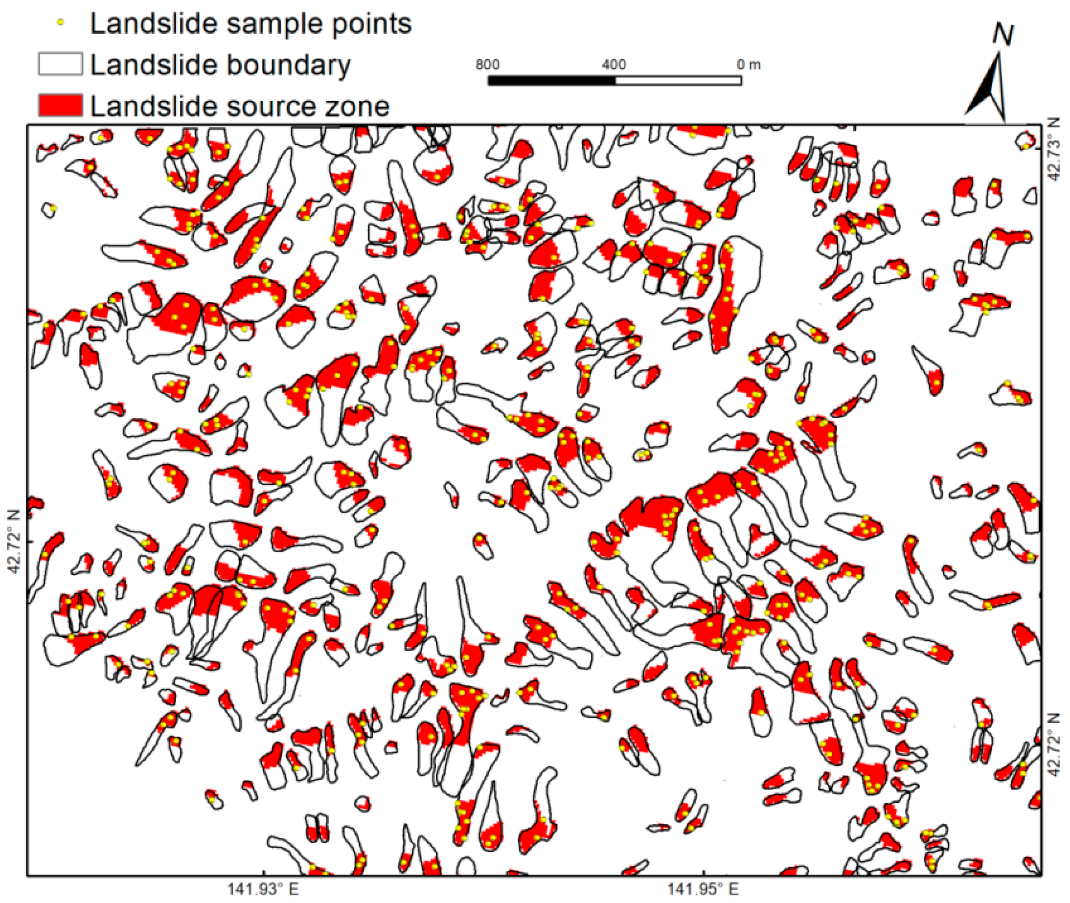
3.1.1. Landslide Inventory
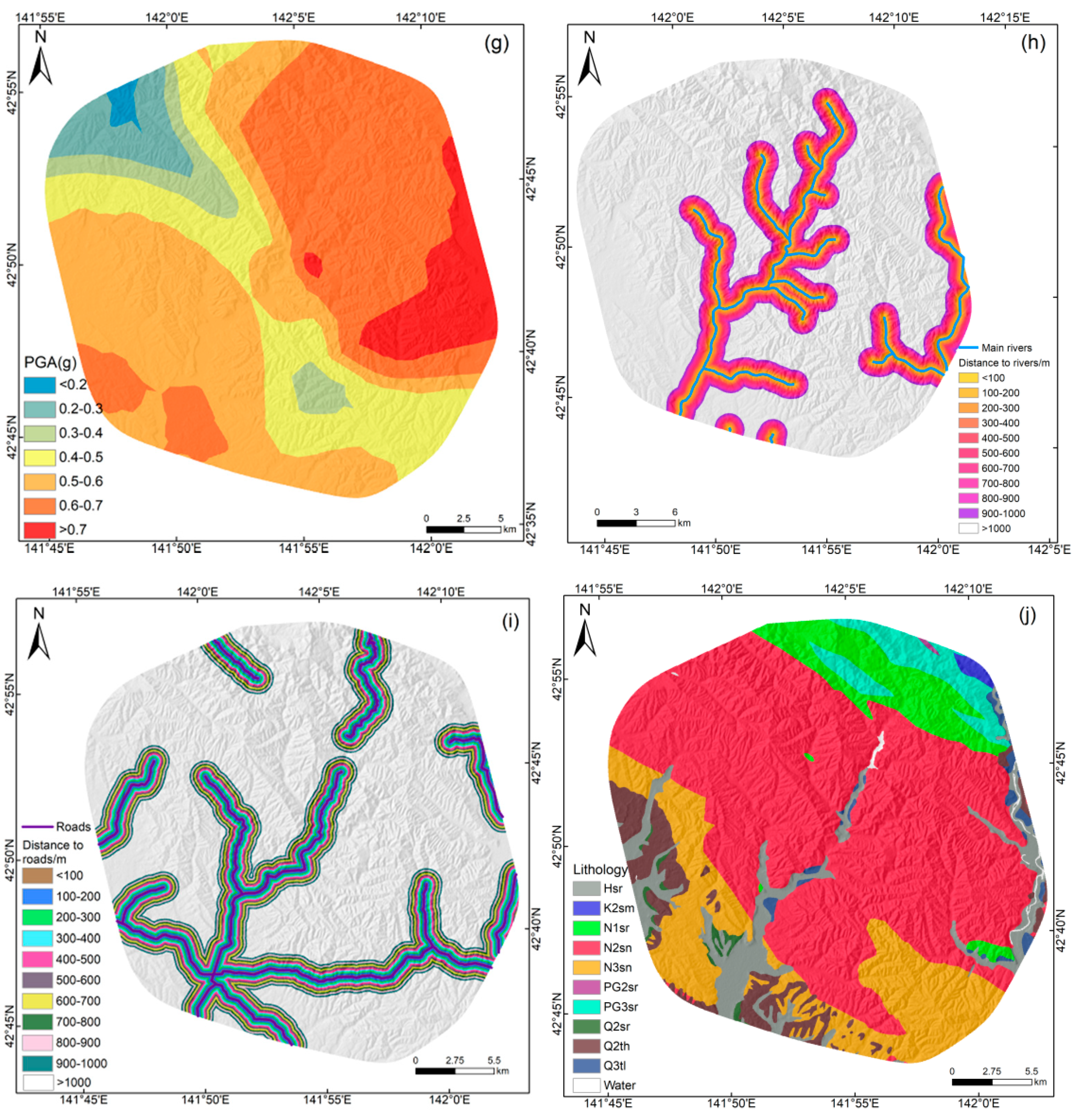
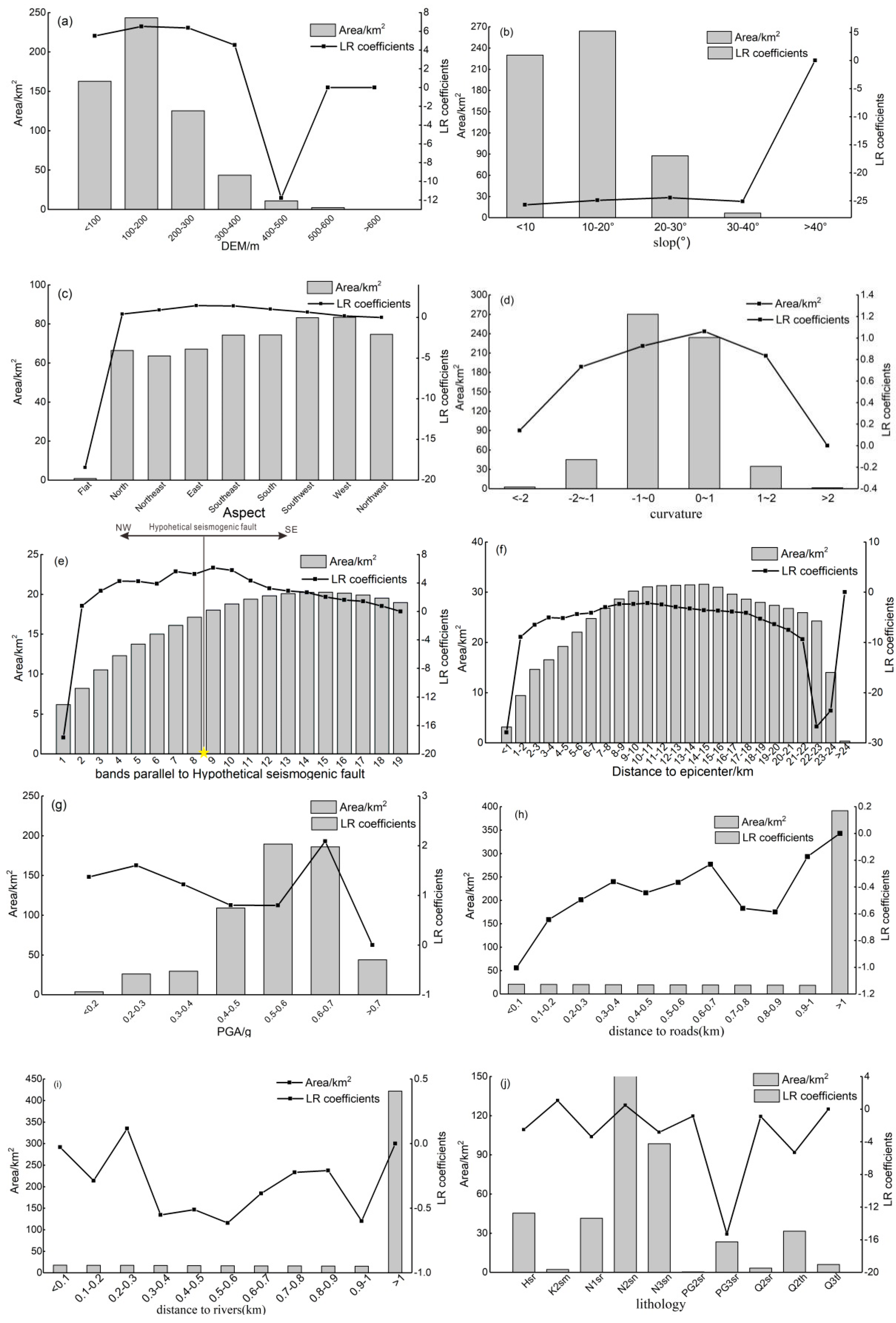
3.1.2. Influencing Factors of Landslide Susceptibility
3.1.3. Sampling Method for Landslide Data
3.2. Methodology
3.2.1. Logistic Regression (LR)
3.2.2. Support Vector Machine (SVM)
4. Results and Analyses
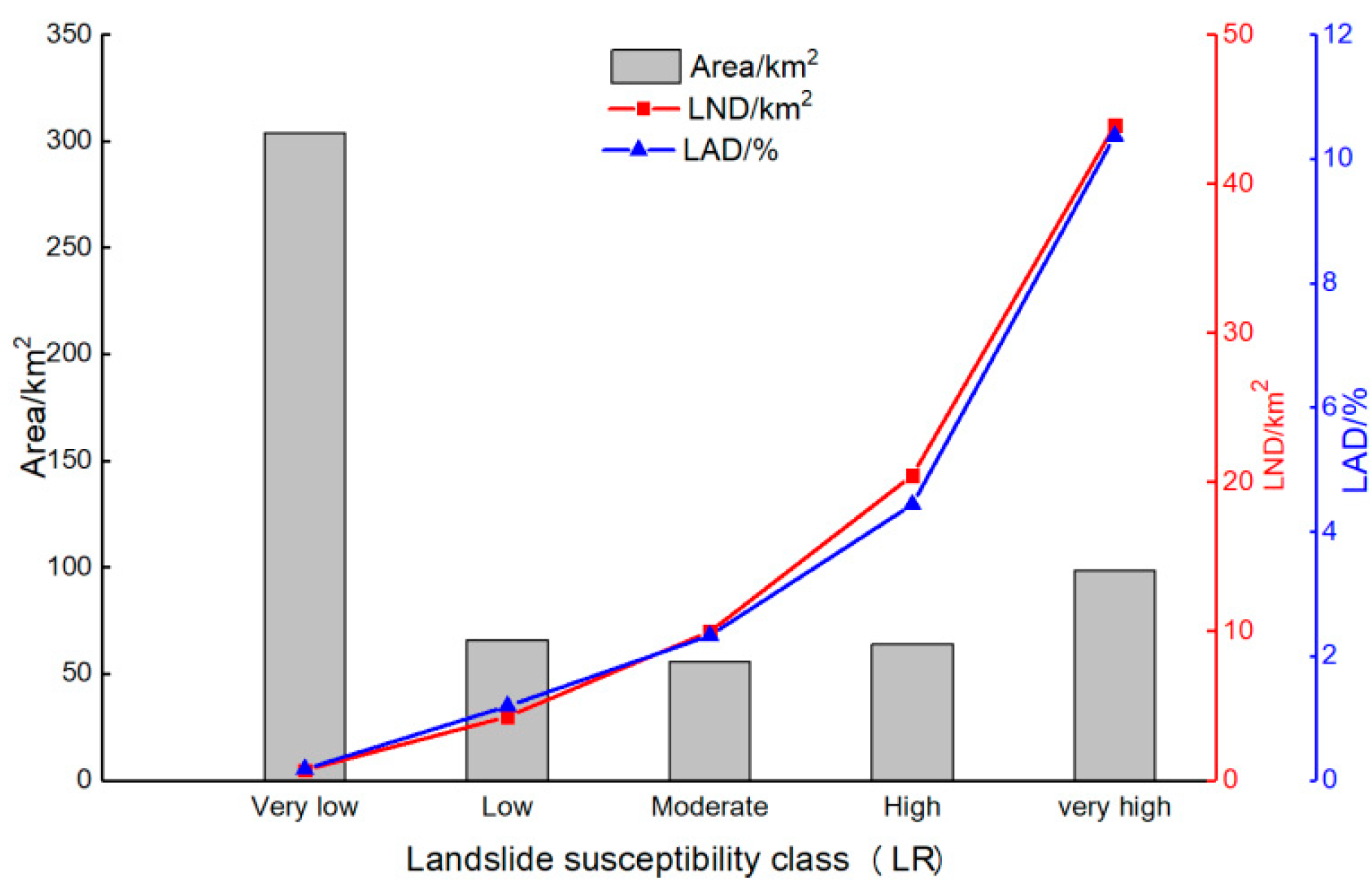
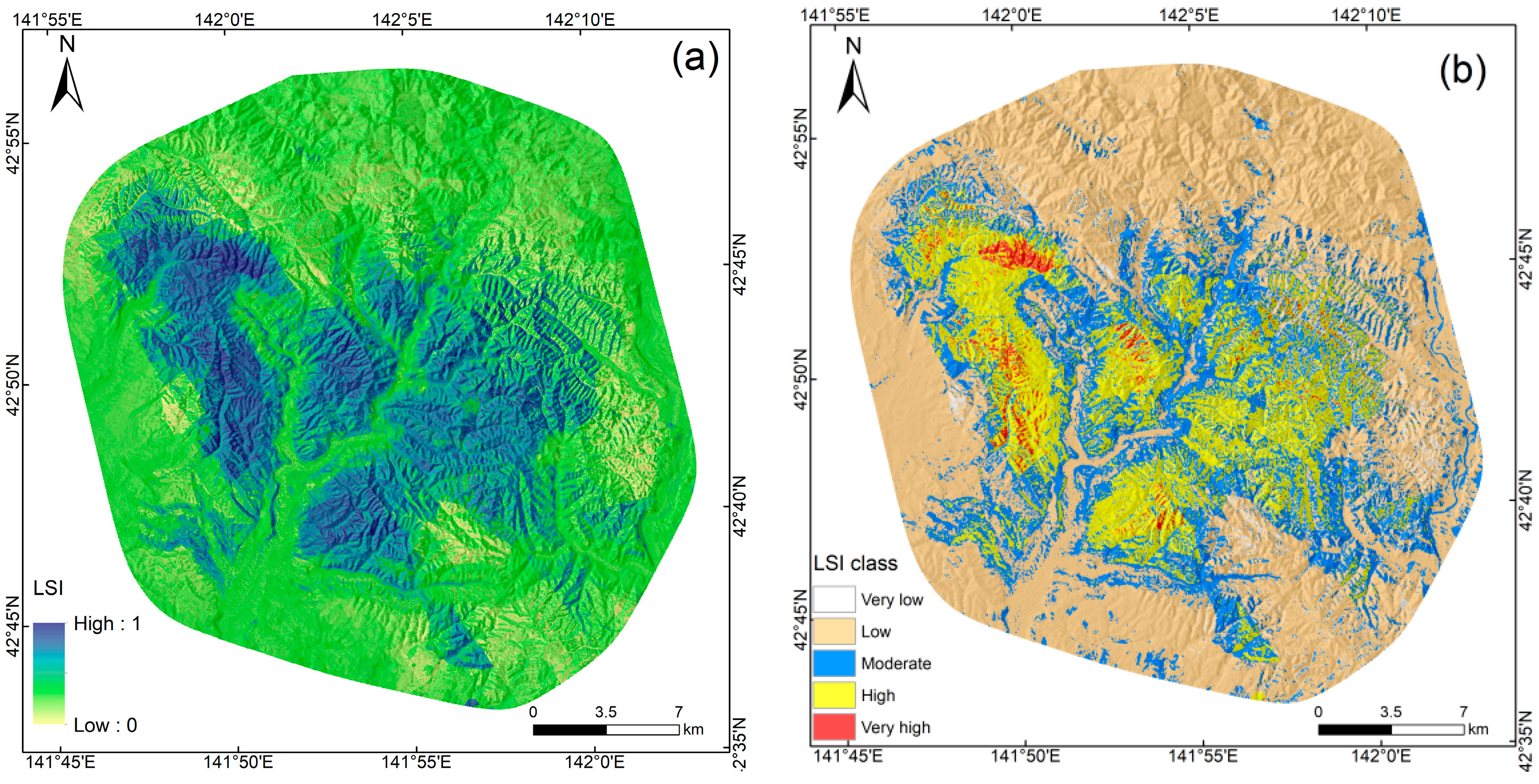
4.1. LSM of LR
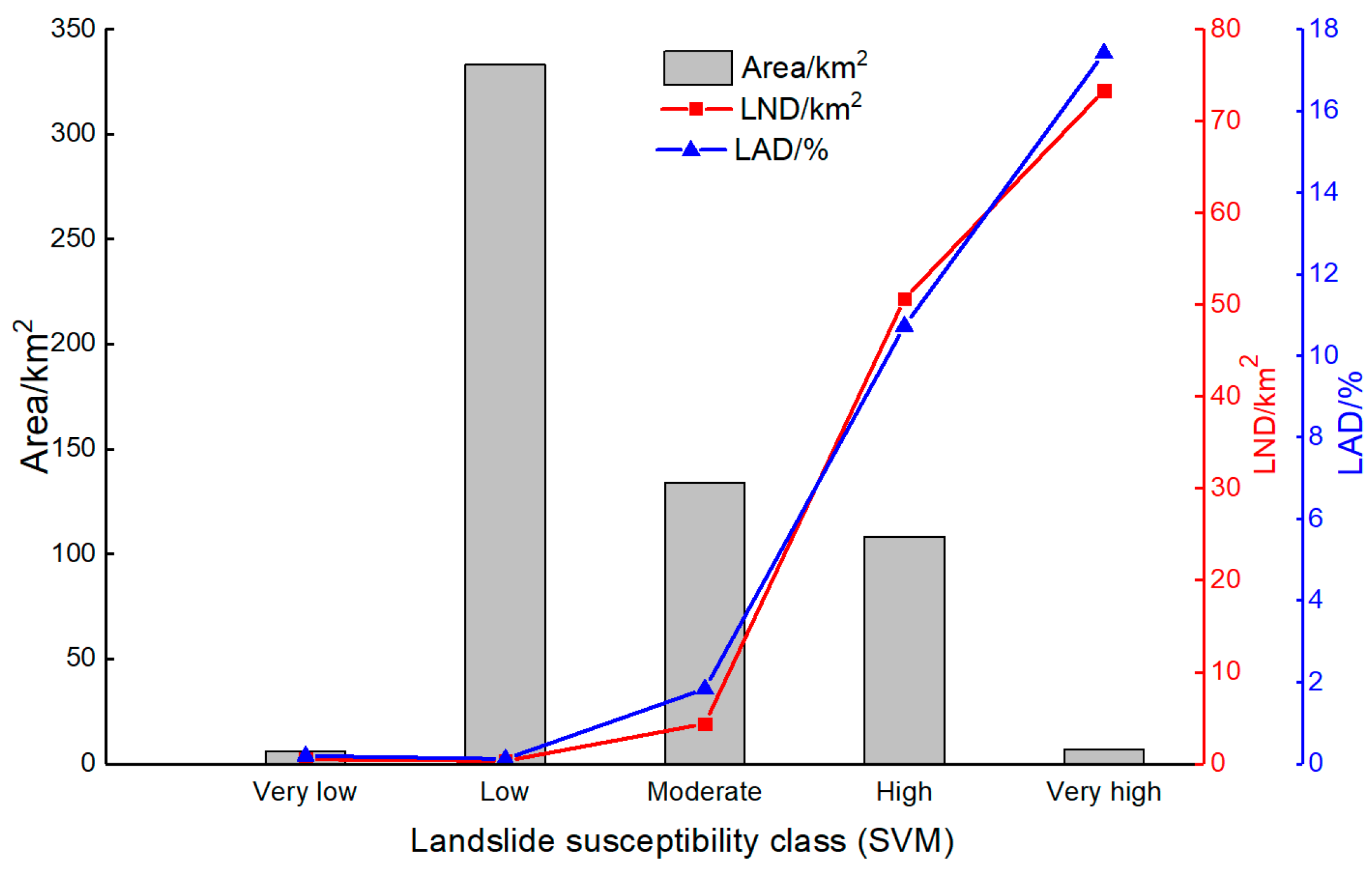
4.2. LSM of SVM
4.3. Model Validation and Quantitative Analysis
5. Discussion
6. Conclusions
Supplementary Materials
Author Contributions
Funding
Acknowledgments
Conflicts of Interest
References
- Dai, F.; Xu, C.; Yao, X.; Xu, L.; Tu, X.; Gong, Q. Spatial distribution of landslides triggered by the 2008 Ms 8.0 Wenchuan earthquake, China. J. Asian Earth Sci. 2011, 40, 883–895. [Google Scholar] [CrossRef]
- Kargel, J.S.; Leonard, G.J.; Shugar, D.H.; Haritashya, U.K.; Bevington, A.; Fielding, E.J.; Fujita, K.; Geertsema, M.; Miles, E.S.; Steiner, J.; et al. Geomorphic and geologic controls of geohazards induced by Nepal’s 2015 Gorkha earthquake. Science 2016, 351, aac8353. [Google Scholar] [CrossRef]
- Yamagishi, H.; Yamazaki, F. Landslides by the 2018 Hokkaido Iburi-Tobu earthquake on September 6. Landslides 2018, 15, 2521–2524. [Google Scholar] [CrossRef]
- Ercanoglu, M.; Kasmer, O.; Temiz, N. Adaptation and comparison of expert opinion to analytical hierarchy process for landslide susceptibility mapping. Bull. Eng. Geol. Environ. 2008, 67, 565–578. [Google Scholar] [CrossRef]
- Guzzetti, F.; Carrara, A.; Cardinali, M.; Reichenbach, P. Landslide hazard evaluation: A review of current techniques and their application in a multi-scale study, Central Italy. Geomorphology 1999, 31, 181–216. [Google Scholar] [CrossRef]
- Agterberg, F.P.; Bonham-Carter, G.F.; Cheng, Q.; Wright, D.F. Weights of evidence modeling and weighted logistic regression for mineral potential mapping. In Computers in Geology, 25 Years of Progress; Oxford University Press: Oxford, UK, 1993; pp. 13–32. [Google Scholar]
- He, S.; Pan, P.; Dai, L.; Wanga, H. Application of kernel-based Fisher discriminant analysis to map landslide susceptibility in the Qinggan River delta, Three Gorges, China. Geomorphology 2012, 172, 30. [Google Scholar] [CrossRef]
- Singh, L.P.; Westen, C.J.V.; Ray, P.K.C.; Pasquali, P. Accuracy assessment of InSAR derived input maps for landslide susceptibility analysis: A case study from the Swiss Alps. Landslides 2005, 2, 221–228. [Google Scholar] [CrossRef]
- Zhou, J.W.; Lu, P.Y.; Hao, M.H. Landslides triggered by the 3 August 2014 Ludian earthquake in China: Geological properties, geomorphologic characteristics and spatial distribution analysis. Geomat. Nat. Hazards Risk 2015, 7, 1–23. [Google Scholar] [CrossRef]
- Xu, C.; Xu, X.; Dai, F.C.; Wu, Z. Application of an incomplete landslide inventory, logistic regression;model and its validation for landslide susceptibility mapping related to;the May 12, 2008 Wenchuan earthquake of China. Nat. Hazards 2013, 68, 883–900. [Google Scholar] [CrossRef]
- Kavzoglu, T.; Sahin, E.K.; Colkesen, I. An assessment of multivariate and bivariate approaches in landslide susceptibility mapping: A case study of Duzkoy district. Nat. Hazards 2015, 76, 471–496. [Google Scholar] [CrossRef]
- Ahmed, B.; Dewan, A. Application of Bivariate and Multivariate Statistical Techniques in Landslide Susceptibility Modeling in Chittagong City Corporation, Bangladesh. Remote Sens. 2017, 9, 304. [Google Scholar] [CrossRef]
- Ayalew, L.; Yamagishi, H. The application of GIS-based logistic regression for landslide susceptibility mapping in the Kakuda-Yahiko Mountains, Central Japan. Geomorphology 2005, 65, 15–31. [Google Scholar] [CrossRef]
- Nowicki, M.A.; Wald, D.J.; Hamburger, M.W.; Hearne, M.; Thompson, E.M. Development of a globally applicable model for near real-time prediction of seismically induced landslides. Eng. Geol. 2014, 173, 54–65. [Google Scholar] [CrossRef]
- Nowicki Jessee, M.A.; Hamburger, M.W.; Allstadt, K.; Wald, D.J.; Robeson, S.M.; Tanyas, H.; Hearne, M.; Thompson, E.M. A Global Empirical Model for Near-Real-Time Assessment of Seismically Induced Landslides. J. Geophys. Res. Earth Surf. 2018. [Google Scholar] [CrossRef]
- Parker, R.N.; Rosser, N.J.; Hales, T.C. Spatial prediction of earthquake-induced landslide probability. Nat. Hazards Earth Syst. Sci. Discuss. 2017, 1–29. [Google Scholar] [CrossRef] [Green Version]
- Dai, F.C.; Lee, C.F. Landslide characteristics and slope instability modeling using GIS, Lantau Island, Hong Kong. Geomorphology 2002, 42, 213–228. [Google Scholar] [CrossRef]
- Aditian, A.; Kubota, T.; Shinohara, Y. Comparison of GIS-based landslide susceptibility models using frequency ratio, logistic regression, and artificial neural network in a tertiary region of Ambon, Indonesia. Geomorphology 2018, 318, 101–111. [Google Scholar] [CrossRef]
- Pradhan, B.; SaRo, L. Landslide susceptibility assessment and factor effect analysis: Backpropagation artificial neural networks and their comparison with frequency ratio and bivariate logistic regression modelling. Environ. Model. Softw. 2010, 25, 747–759. [Google Scholar] [CrossRef]
- Yao, X.; Tham, L.G.; Dai, F.C. Landslide susceptibility mapping based on Support Vector Machine: A case study on natural slopes of Hong Kong, China. Geomorphology 2008, 101, 572–582. [Google Scholar] [CrossRef]
- Tien Bui, D.; Shahabi, H.; Shirzadi, A.; Chapi, K.; Hoang, N.-D.; Pham, B.; Bui, Q.-T.; Tran, C.-T.; Panahi, M.; Bin Ahamd, B.; et al. A Novel Integrated Approach of Relevance Vector Machine Optimized by Imperialist Competitive Algorithm for Spatial Modeling of Shallow Landslides. Remote Sens. 2018, 10, 1538. [Google Scholar] [CrossRef]
- Tien Bui, D.; Shahabi, H.; Shirzadi, A.; Chapi, K.; Alizadeh, M.; Chen, W.; Mohammadi, A.; Ahmad, B.; Panahi, M.; Hong, H.; et al. Landslide Detection and Susceptibility Mapping by AIRSAR Data Using Support Vector Machine and Index of Entropy Models in Cameron Highlands, Malaysia. Remote Sens. 2018, 10, 1527. [Google Scholar] [CrossRef]
- Zhou, C.; Yin, K.; Cao, Y.; Ahmed, B.; Li, Y.; Catani, F.; Pourghasemi, H.R. Landslide susceptibility modeling applying machine learning methods: A case study from Longju in the Three Gorges Reservoir area, China. Comput. Geosci. 2018, 112, 23–37. [Google Scholar] [CrossRef]
- Xu, C.; Shen, L.; Wang, G. Soft computing in assessment of earthquake-triggered landslide susceptibility. Environ. Earth Sci. 2016, 75. [Google Scholar] [CrossRef]
- Xu, C.; Dai, F.; Xu, X.; Yuan, H.L. GIS-based support vector machine modeling of earthquake-triggered landslide susceptibility in the Jianjiang River watershed, China. Geomorphology 2012, 145–146, 70–80. [Google Scholar] [CrossRef]
- Zhou, S.; Fang, L. Support vector machine modeling of earthquake-induced landslides susceptibility in central part of Sichuan province, China. Geoenviron. Disasters 2015, 2, 1–12. [Google Scholar] [CrossRef]
- Xu, C.; Xu, X.; Dai, F.; Saraf, A.K. Comparison of different models for susceptibility mapping of earthquake triggered landslides related with the 2008 Wenchuan earthquake in China. Comput. Geosci. 2012, 46, 317–329. [Google Scholar] [CrossRef]
- Active fault research group. Active Faults in Japan: Sheet Maps and Inventories (Revised Edition); University of Tokyo Press: Tokyo, Janpan, 1991. [Google Scholar] [CrossRef]
- Nakata, T. Digital Active Fault Map of Japan; University of Tokyo Press: Tokyo, Japan, 2002. [Google Scholar] [CrossRef]
- Amante, C.; Eakins, B. ETOPO1 1 Arc-Minute Global Relief Model: Procedures, Data Sources and Analysis; US Department of Commerce: Alexandria, VA, USA; National Oceanic and Atmospheric Administration: Silver Spring, MD, USA; National Environmental Satellite, Data, and Information Service: Silver Spring, MD, USA; National Geophysical Data Center Marine Geology and Geophysics Division: Boulder, CO, USA, 2009. Available online: https://www.ngdc.noaa.gov/mgg/global/relief/ETOPO1/docs/ETOPO1.pdf (accessed on 10 January 2019). [CrossRef]
- Xu, C.; Xu, X.; Yao, X.; Dai, F. Three (nearly) complete inventories of landslides triggered by the May 12, 2008 Wenchuan Mw 7.9 earthquake of China and their spatial distribution statistical analysis. Landslides 2014, 11, 441–461. [Google Scholar] [CrossRef]
- Xu, C.; Xu, X.; Shyu, J.B.H. Database and spatial distribution of landslides triggered by the Lushan, China Mw 6.6 earthquake of 20 April 2013. Geomorphology 2015, 248, 77–92. [Google Scholar] [CrossRef] [Green Version]
- Planet Team. Planet Application Program Interface: In Space for Life on Earth; Planet Company: San Francisco, CA, USA, 2018; Available online: https://api.planet.com (accessed on 10 January 2019). [CrossRef]
- Sato, H.P.; Harp, E.L. Interpretation of earthquake-induced landslides triggered by the 12 May 2008, M7.9 Wenchuan earthquake in the Beichuan area, Sichuan Province, China using satellite imagery and Google Earth. Landslides 2009, 6, 153–159. [Google Scholar] [CrossRef]
- Yalcin, A. GIS-based landslide susceptibility mapping using analytical hierarchy process and bivariate statistics in Ardesen (Turkey): Comparisons of results and confirmations. CATENA 2008, 72, 1–12. [Google Scholar] [CrossRef]
- Chen, X.L.; Liu, C.G.; Yu, L.; Lin, C.X. Critical acceleration as a criterion in seismic landslide susceptibility assessment. Geomorphology 2014, 217, 15–22. [Google Scholar] [CrossRef]
- Geological Survey of Japan, A.E. Research Information Database DB084, Geological Survey of Japan, Jul 3, 2012 Version; Geological Survey of Japan, National Institute of Advanced Industrial Science and Technology: Tokyo, Japan, 2012. [CrossRef]
- Xu, Q.; Zhang, S.; Li, W. Spatial distribution of large-scale landslides induced by the 5.12 Wenchuan Earthquake. J. Mt. Sci. 2011, 8, 246. [Google Scholar] [CrossRef]
- Xu, C.; Xu, X.; Yu, G.J.L. Landslides triggered by slipping-fault-generated earthquake on a plateau: An example of the 14 April 2010, Ms 7.1, Yushu, China earthquake. Landslides 2013, 10, 421–431. [Google Scholar] [CrossRef]
- Bai, S.B.; Lu, P.; Wang, J. Landslide susceptibility assessment of the Youfang catchment using logistic regression. J. Mt. Sci. 2015, 12, 816–827. [Google Scholar] [CrossRef]
- Cortes, C.; Vapnik, V. Support-vector networks. Mach. Learn. 1995, 20, 273–297. [Google Scholar] [CrossRef] [Green Version]
- Li, X.; Cheng, X.; Chen, W.; Chen, G.; Liu, S. Identification of Forested Landslides Using LiDar Data, Object-based Image Analysis, and Machine Learning Algorithms. Remote Sens. 2015, 7, 9705–9726. [Google Scholar] [CrossRef] [Green Version]
- Marjanović, M.; Kovačević, M.; Bajat, B.; Voženílek, V. Landslide susceptibility assessment using SVM machine learning algorithm. Eng. Geol. 2011, 123, 225–234. [Google Scholar] [CrossRef]
- Bui, D.T.; Revhaug, I.; Dick, O. Landslide susceptibility analysis in the Hoa Binh province of Vietnam using statistical index and logistic regression. Nat. Hazards 2011, 59, 1413–1444. [Google Scholar] [CrossRef]
- Chang, C.C.; Lin, C.J. LIBSVM: A library for support vector machines. Acm Trans. Intell. Syst. Technol. 2011, 2, 1–27. [Google Scholar] [CrossRef]
- Brenning, A. Spatial prediction models for landslide hazards: Review, comparison and evaluation. Nat. Hazards Earth Syst. Sci. 2005, 5, 853–862. [Google Scholar] [CrossRef]
- Cao, J.; Zhang, Z.; Wang, C.; Liu, J.; Zhang, L. Susceptibility assessment of landslides triggered by earthquakes in the Western Sichuan Plateau. CATENA 2019, 175, 63–76. [Google Scholar] [CrossRef]
- Bai, S.B.; Wang, J.; Lü, G.N.; Zhou, P.G.; Hou, S.S.; Xu, S.N. GIS-based logistic regression for landslide susceptibility mapping of the Zhongxian segment in the Three Gorges area, China. Geomorphology 2010, 115, 23–31. [Google Scholar] [CrossRef]
- Akgun, A. A comparison of landslide susceptibility maps produced by logistic regression, multi-criteria decision, and likelihood ratio methods: A case study at İzmir, Turkey. Landslides 2012, 9, 93–106. [Google Scholar] [CrossRef]
- Pradhan, B. Manifestation of an advanced fuzzy logic model coupled with Geo-information techniques to landslide susceptibility mapping and their comparison with logistic regression modelling. Environ. Ecol. Stat. 2011, 18, 471–493. [Google Scholar] [CrossRef]
- Roback, K.; Clark, M.K.; West, A.J.; Zekkos, D.; Li, G.; Gallen, S.F.; Chamlagain, D.; Godt, J.W. The size, distribution, and mobility of landslides caused by the 2015 Mw7.8 Gorkha earthquake, Nepal. Geomorphology 2018, 301, 121–138. [Google Scholar] [CrossRef]
- Ma, S.; Xu, C. Assessment of co-seismic landslide hazard using the Newmark model and statistical analyses: A case study of the 2013 Lushan, China, Mw6.6 earthquake. Nat. Hazards 2018. [Google Scholar] [CrossRef]


| Latitude (°) | Longitude (°) | Dip (°) | Depth (km) | Rake (°) | Mo (Nm) | Var. Red. | Strike (°) |
|---|---|---|---|---|---|---|---|
| 42.6908 | 142.0067 | 30; 65 | 35 | 59; 107 | 1e + 19 | 89.47 | 134; 349 |
| Classification | Regression Coefficients | Classification | Regression Coefficient | Classification | Regression Coefficients |
|---|---|---|---|---|---|
| <DEM> | 11 | 4.321 | 7: >0.7g | 0 | |
| 1: <100 m | 5.51 | 12 | 3.238 | <Distances to roads> | |
| 2:100–200 m | 6.524 | 13 | 2.892 | 1:<100 m | −1.005 |
| 3:200–300 m | 6.364 | 14 | 2.68 | 2:100–200 m | −0.644 |
| 4:300–400 m | 4.532 | 15 | 2.027 | 3:200–300 m | −0.496 |
| 5:400–500 m | −11.78 | 16 | 1.607 | 4:300–400 m | −0.361 |
| 6:500–600 m | 0 | 17 | 1.429 | 5:400–500 m | −0.444 |
| 7:>600 m | 0 | 18 | 0.755 | 6:500–600 m | −0.366 |
| <Slope angle> | 19 | 0 | 7:600–700 m | −0.231 | |
| 1:<10° | −25.717 | <Distances to epicenter> | 8:700–800 m | −0.56 | |
| 2:10–20° | −24.894 | 1 | −27.93 | 9:800–900 m | −0.587 |
| 3:20–30° | −24.426 | 2 | −8.91 | 10:900–1000 m | −0.173 |
| 4:30–40° | −25.102 | 3 | −6.511 | 11: >1000 m | 0 |
| 5:>40° | 0 | 4 | −5.07 | <Distance to rivers> | |
| <Aspect> | 5 | −5.185 | 1: <100 m | −0.028 | |
| 1: Flat | −18.45 | 6 | −4.388 | 2:100–200 m | −0.287 |
| 2: North | 0.416 | 7 | −4.125 | 3:200–300 m | 0.116 |
| 3: Northeast | 0.92 | 8 | −2.974 | 4:300–400 m | −0.552 |
| 4: East | 1.454 | 9 | −2.353 | 5:400–500 m | −0.511 |
| 5: Southeast | 1.423 | 10 | −2.379 | 6:500–600 m | −0.614 |
| 6: South | 1.021 | 11 | −2.185 | 7:600–700 m | −0.386 |
| 7: Southwest | 0.652 | 12 | −2.474 | 8:700–800 m | −0.222 |
| 8: West | 0.187 | 13 | −2.956 | 9:800–900 m | −0.209 |
| 9: Northwest | 0 | 14 | −3.254 | 10:900–1000 m | −0.6 |
| <Curvature> | 15 | −3.59 | 11:>1000 m | 0 | |
| 1: <−2 | 0.14 | 16 | −3.692 | <Lithology> | |
| 2: −2~−1 | 0.732 | 17 | −3.897 | 1: Hsr | −2.517 |
| 3: −1~0 | 0.926 | 18 | −4.128 | 2: K2sm | 1.048 |
| 4:0~1 | 1.061 | 19 | −5.292 | 3: N1sr | −3.386 |
| 5:1~2 | 0.834 | 20 | −6.396 | 4: N2sn | 0.486 |
| 6: >2 | 0 | 21 | −7.523 | 5: N3sn | −2.831 |
| <Distances to fault> | 22 | −9.391 | 6: PG2sr | −0.852 | |
| 1 | −17.689 | 23 | −26.766 | 7: PG3sr | −15.327 |
| 2 | 0.766 | 24 | −23.596 | 8: Q2sr | −0.889 |
| 3 | 2.891 | 25 | 0 | 9: Q2th | −5.309 |
| 4 | 4.263 | <PGA> | 10: Q3tl | 0 | |
| 5 | 4.229 | 1: <0.2g | 1.369 | Constant | 17.594 |
| 6 | 3.889 | 2:0.2–0.3g | 1.604 | ||
| 7 | 5.634 | 3:0.3–0.4g | 1.22 | ||
| 8 | 5.249 | 4:0.4–0.5g | 0.8 | ||
| 9 | 6.142 | 5:0.5–0.6g | 0.798 | ||
| 10 | 5.794 | 6:0.6–0.7g | 2.089 | ||
| Area/km2 | Area of Classification/(%) | Number of Landslides | LND/km2 | LAD/(%) | |
|---|---|---|---|---|---|
| Very low | 303.96 | 51.68 | 209 | 0.68 | 0.18 |
| Low | 66.06 | 11.23 | 283 | 4.28 | 1.19 |
| Moderate | 55.52 | 9.44 | 554 | 9.97 | 2.33 |
| High | 63.91 | 10.86 | 1307 | 20.44 | 4.43 |
| Very high | 98.60 | 16.76 | 4329 | 43.90 | 10.37 |
| Area/km2 | Area of Classification/(%) | Number of Landslides | LND/km2 | LAD/(%) | |
|---|---|---|---|---|---|
| Very low | 5.92 | 1.00 | 3 | 0.50 | 0.19 |
| Low | 332.96 | 56.61 | 103 | 0.30 | 0.12 |
| Moderate | 133.98 | 22.78 | 587 | 4.38 | 1.83 |
| High | 108.31 | 18.41 | 5484 | 50.62 | 10.72 |
| Very high | 6.88 | 1.17 | 505 | 73.29 | 17.41 |
© 2019 by the authors. Licensee MDPI, Basel, Switzerland. This article is an open access article distributed under the terms and conditions of the Creative Commons Attribution (CC BY) license (http://creativecommons.org/licenses/by/4.0/).
Share and Cite
Shao, X.; Ma, S.; Xu, C.; Zhang, P.; Wen, B.; Tian, Y.; Zhou, Q.; Cui, Y. Planet Image-Based Inventorying and Machine Learning-Based Susceptibility Mapping for the Landslides Triggered by the 2018 Mw6.6 Tomakomai, Japan Earthquake. Remote Sens. 2019, 11, 978. https://0-doi-org.brum.beds.ac.uk/10.3390/rs11080978
Shao X, Ma S, Xu C, Zhang P, Wen B, Tian Y, Zhou Q, Cui Y. Planet Image-Based Inventorying and Machine Learning-Based Susceptibility Mapping for the Landslides Triggered by the 2018 Mw6.6 Tomakomai, Japan Earthquake. Remote Sensing. 2019; 11(8):978. https://0-doi-org.brum.beds.ac.uk/10.3390/rs11080978
Chicago/Turabian StyleShao, Xiaoyi, Siyuan Ma, Chong Xu, Pengfei Zhang, Boyu Wen, Yingying Tian, Qing Zhou, and Yulong Cui. 2019. "Planet Image-Based Inventorying and Machine Learning-Based Susceptibility Mapping for the Landslides Triggered by the 2018 Mw6.6 Tomakomai, Japan Earthquake" Remote Sensing 11, no. 8: 978. https://0-doi-org.brum.beds.ac.uk/10.3390/rs11080978