Article

Evaluation of Sentinel-1 and 2 Time Series for Land Cover Classification of Forest–Agriculture Mosaics in Temperate and Tropical Landscapes

1
LETG Rennes UMR 6554 LETG, Université Rennes 2, Place du recteur Henri Le Moal, 35043 Rennes CEDEX, France
2
CIRAD, Forêts et Sociétés, F-34398 Montpellier, France
3
Forêts et Sociétés, Univ Montpellier, CIRAD, 34398 Montpellier, France
4
Ecosystems Modelling Unity, Forests, Biodiversity and Climate Change Program, Tropical Agricultural Research and Higher Education Center (CATIE), Turrialba, Cartago 30501, Costa Rica
5
CIRAD, UMR TETIS, F-34398 Montpellier, France
6
TETIS, Univ Montpellier, AgroParisTech, CIRAD, CNRS, IRSTEA, F-34000 Montpellier, France
7
INRA, UMR BAGAP, 65 rue de St-Brieuc CS 84215, 35042 Rennes CEDEX, France
8
ECOGESFOR Research Group, ETSI Montes, Forestal y del Medio Natural, Technical University of Madrid, Ciudad Universitaria s/n, 28040 Madrid, Spain
9
Departamento de Ingeniería y Morfología del Terreno, Universidad Politécnica de Madrid, E-28040 Madrid, Spain
10
Joint Research Unit SELMET (Systèmes d’élevage méditerranéens et tropicaux), CIRAD-Napt Embrapa Belem Brasilia, Bairro Nova Conquista, Paragominas PA 68627-451, Brazil
*
Author to whom correspondence should be addressed.
Submission received: 20 March 2019 / Revised: 17 April 2019 / Accepted: 17 April 2019 / Published: 24 April 2019
(This article belongs to the Special Issue Remote Sensing of Tropical Environmental Change)

Abstract

:
Monitoring forest–agriculture mosaics is crucial for understanding landscape heterogeneity and managing biodiversity. Mapping these mosaics from remotely sensed imagery remains challenging, since ecological gradients from forested to agricultural areas make characterizing vegetation more difficult. The recent synthetic aperture radar (SAR) Sentinel-1 (S-1) and optical Sentinel-2 (S-2) time series provide a great opportunity to monitor forest–agriculture mosaics due to their high spatial and temporal resolutions. However, while a few studies have used the temporal resolution of S-2 time series alone to map land cover and land use in cropland and/or forested areas, S-1 time series have not yet been investigated alone for this purpose. The combined use of S-1 & S-2 time series has been assessed for only one or a few land cover classes. In this study, we assessed the potential of S-1 data alone, S-2 data alone, and their combined use for mapping forest–agriculture mosaics over two study areas: a temperate mountainous landscape in the Cantabrian Range (Spain) and a tropical forested landscape in Paragominas (Brazil). Satellite images were classified using an incremental procedure based on an importance rank of the input features. The classifications obtained with S-2 data alone (mean kappa index = 0.59–0.83) were more accurate than those obtained with S-1 data alone (mean kappa index = 0.28–0.72). Accuracy increased when combining S-1 and 2 data (mean kappa index = 0.55–0.85). The method enables defining the number and type of features that discriminate land cover classes in an optimal manner according to the type of landscape considered. The best configuration for the Spanish and Brazilian study areas included 5 and 10 features, respectively, for S-2 data alone and 10 and 20 features, respectively, for S-1 data alone. Short-wave infrared and VV and VH polarizations were key features of S-2 and S-1 data, respectively. In addition, the method enables defining key periods that discriminate land cover classes according to the type of images used. For example, in the Cantabrian Range, winter and summer were key for S-2 time series, while spring and winter were key for S-1 time series.

1. Introduction

Mapping forest–agriculture mosaics is essential for understanding effects of land cover changes on economic (e.g., agricultural and silvicultural production, timber extraction, ecotourism) and non-market ecosystem services (e.g., carbon sequestration, water quality, stream flow, species conservation) [1]. Cropland and pastures are the largest use of Earth’s ice-free land [2] and have particularly high biodiversity potential [3]. However, this capacity refers to landscapes with heterogeneous semi-intensive agricultural systems and semi-natural elements (hedgerows, wetlands, forests) [4,5,6]. In many parts of the world, land cover changes affect landscapes, causing habitat loss and fragmentation [7]. Habitat fragmentation decreases the size of habitats and populations and increases distances between patches of habitat, which may result in species loss [8].
Each species uses different kinds of habitats and requires different amounts of them [7]. Many species perceive landscapes in ways more complex than as a “habitat-matrix” dichotomy (i.e., dividing the landscape into “habitat”, which contains all necessary resources, and “matrix”, which is hostile) and use resources from different cover types [5]. Thus, landscape management can be considered a complex process that requires characterizing the landscape composition and structure suitable for the target species. Habitat selection and resistance models are widely used as a decision support tool, since they can apply to multiple groups of species (e.g., insects, birds, herpetofauna, mammals, plants). Landscape maps are essential for developing these models, and most environmental features used in the models are derived from remote sensing imagery [9]. Remotely sensed imagery is a common tool for straightforward land cover classification. The main difficulty is that the land cover classes in forest–agriculture mosaics are distributed along a landscape gradient, which results in misclassification. Images with high and very high spatial resolutions provide greater spatial detail and precise information [10,11,12,13]. However, the low temporal resolution of such data does not enable monitoring vegetation dynamics to better discriminate land cover classes that are spectrally similar. In contrast, satellite time series provide great opportunities for this purpose.
MODIS and Landsat optical time series have been used extensively for land cover classification since the 1970s. Despite a 1–2-day revisit time, however, land cover derived from MODIS has low local accuracy due to the maximum spatial resolution of 250 m. The Landsat constellation has an 8-day revisit time but has a higher spatial resolution (30 m) than MODIS. The S-2 satellite has even higher capacities, with a five-day revisit time and a 10 m spatial resolution [14]. Despite these high capacities, optical images sometimes cannot be used (e.g., lack of cloud-free periods) or are at the limit of their utility (e.g., optical reflectance provides information only about the top layer of vegetation). In this context, synthetic aperture radar (SAR) images provide a reliable alternative to optical images because they are not greatly influenced by atmospheric conditions and can be acquired during the day or night. Several scattering mechanisms, including single bounce, double bounce, and volume scattering can contribute to SAR backscatter over distributed targets such as agricultural fields [15], depending on crop properties (e.g., biomass, architecture, height) [16,17,18] and soil conditions (e.g., roughness, moisture) [19,20,21]. Unlike optical data, however, SAR data are rarely used to map land cover. Some studies have focused on the complementarity of SAR and optical data, concluding that using them together provided better results than using them separately [22]. The SAR signal is sensitive to the geometry (e.g., roughness, texture, internal structure) and wetness of the observed targets, while optical reflectance is influenced by their physiology. Thus, these two spectral domains provide complementary information.
The recent SAR Sentinel-1 (S-1) and optical Sentinel-2 (S-2) time series provide a great opportunity to monitor forest–agriculture mosaics due to their high spatial and temporal resolutions, with a five-day revisit time and decametric resolution. They are freely available under an open license, unlike most SAR data (e.g., TerraSAR-X, ALOS2, RADARSAT-2, COSMO-Sky Med) and optical data (e.g., SPOT, Quickbird, WorldView, Geo-Eye, Ikonos). Recent studies have demonstrated the potential of S-2 data for mapping 6–12 land cover classes from a single-date image [23,24,25,26,27]. Studies that use S-2 time series focus on one or a few specific land cover classes, usually on homogeneous agricultural or forested landscapes located in the same climatic region [28,29,30,31,32,33,34]. Use of S-1 data has been limited to combining them with S-2 or Landsat data, which increases classification accuracy [35,36,37,38,39]. Hence, the use of S-1 time series alone for mapping land cover classes has not yet been evaluated.
The objective of this study was to assess the potential of S-1 data alone, S-2 data alone, and combined S-1 and 2 data for mapping land cover in forest–agriculture mosaics. We focused on two landscapes with contrasting vegetation gradients: a temperate mountainous landscape in the Cantabrian Range (Spain) and a humid tropical forested landscape in Paragominas (Brazil). Although these forest–agriculture mosaics differ greatly, they perform similar ecological functions, such as conserving high levels of biodiversity and storing carbon.
Satellite images were classified using an incremental procedure based on the rank of importance of input features derived from S-1 and S-2 time series. The method automatically selects the relevant features (spectral bands and/or vegetation indices) and time periods to use to best classify land cover types in the forest–agriculture mosaics.

2. Study Area and Data
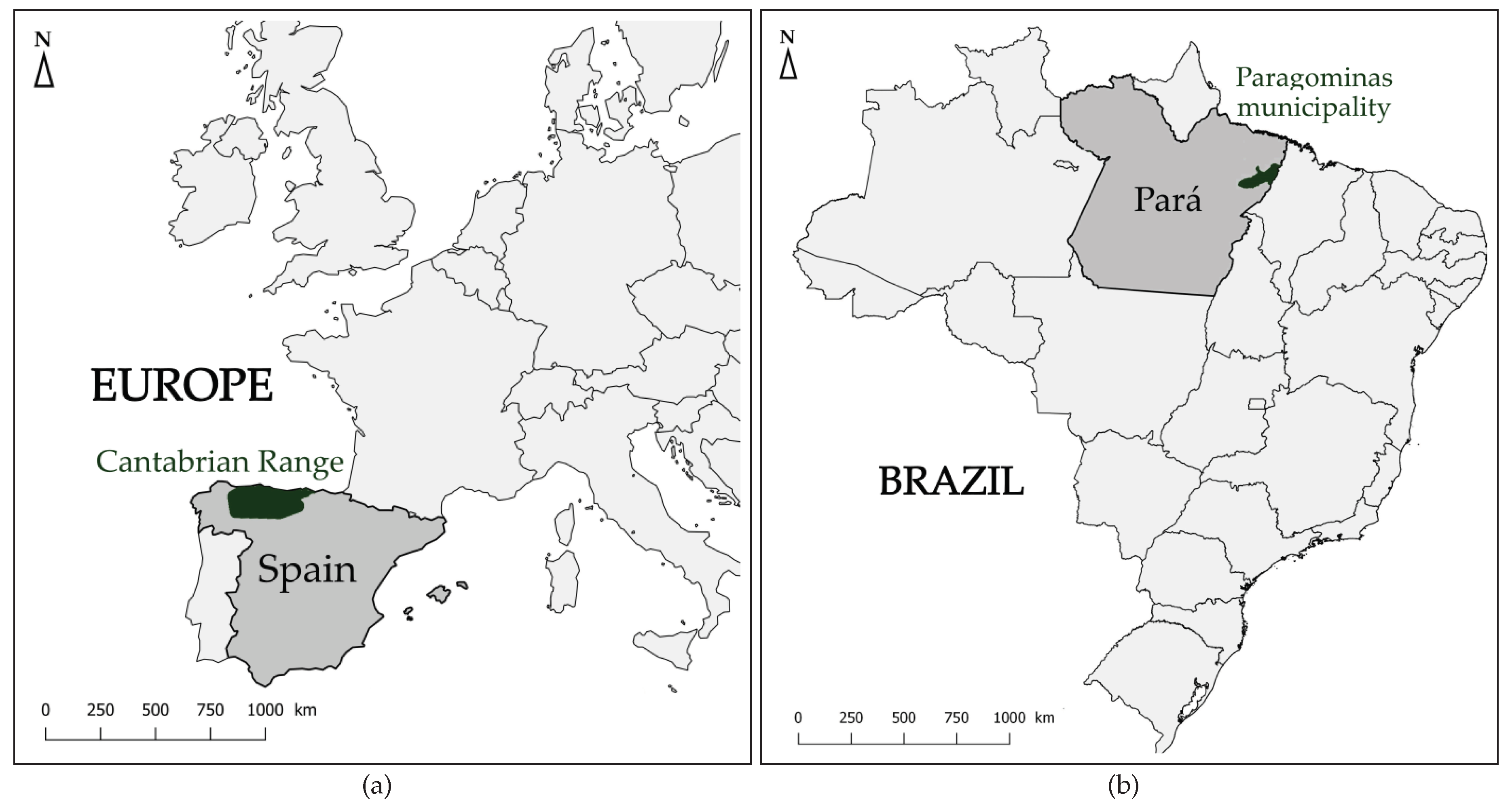
2.1. Study Area

The Spanish study area is located in northwestern Spain, extending from eastern Lugo to western Cantabria. Covering the entire Cantabrian Range, it has an area of 35,700 km 2 (Figure 1a). The region has an elevation of 0–2468 m, an Atlantic climate, and remnant forest fragments that are distinct from a non-forest matrix composed mainly of pastures and heathlands in abandoned meadows [40,41]. Croplands constitute 22% of the study area and are composed of vines and cereals crops including wheat, barley, rye, sunflower and oats [42]. These crops are located in the south of the study area (Castile-Leon), most of them are irrigated [43]. In northern slopes of the Cantabrian range, oaks (Quercus robur and Q. petraea), beeches (Fagus sylvatica) and chestnuts (Castanea sativa) are the main species found in forested areas, while southern slopes are dominated by semi-deciduous oaks (Q. pyrenaica and Q. faginea) and evergreen oaks (Q. ilex), Pinus sp. and Eucalyptus globulus being relatively abundant [42]. The major decrease in the forest area dates back to 3000 years BP, with the transformation of large patches of natural forests into pasturelands (traditional cattle grazing and selective timber extraction). More recently, additional forests were lost due to road construction, surface mining, increased frequency of anthropogenic fires, and creation of forest plantations. In the past 20 years, reserves were established that impose legal restrictions on new land uses [40]. Many studies focused on habitat quality for brown bear and wood grouse, two native species of the Cantabrian Range, indicating that the forest cover is essential to their presence [41,44]. Brown bear home ranges include forests, shrublands, rocky areas, and grasslands [41].
The second study area is the municipality of Paragominas, Pará State, in the eastern Brazilian Amazonia, 217 km south of Belem (Figure 1b). The municipality extends for 19,342 km 2 , has an elevation up to 190 m, and has a tropical climate. It experienced a continuous period of deforestation from the 1960s to 2010, due mainly to cattle ranching, soybean and corn cultivation, and creation of forest plantations. Overlogging and fires degraded the remaining forests greatly [45,46]. The municipality was the main timber-producing region in Brazil in 1990. A biodiversity survey performed in the municipality showed that both landscape and within-forest disturbances contributed to biodiversity loss, with the greatest negative effects on species of high conservation and functional value [47]. In 2005, in the context of the new federal policy to fight deforestation, Paragominas was asked to establish measures against deforestation. The municipality established a new local governance model, called “Municipio Verde” [48], which aimed to fight deforestation and strengthen the ability of local institutions to develop specific environmental policies based on the Brazilian forest code. Since then, annual deforestation rates have decreased by up to 80%. Paragominas represents a case of remarkable deforestation that became a national reference for municipal-level anti-deforestation policies.

2.2. Data

2.2.1. Reference Data

A set of 828 polygons was manually discriminated on the Spanish study area using aerial photographs and the Forest Map of Spain [49], which was developed from 1997–2006 and is the official forest inventory of the country. Its minimum mapping unit is 2.25 ha. The map is composed of polygons containing land cover and land use attributes derived from interpretation of aerial photographs and field inventory data. The 8 land cover classes discriminated in the sample data were permanent bare soils, artificial surfaces, water bodies, forested areas, shrublands, permanent herbaceous vegetation (herbaceous vegetation containing chlorophyll throughout the year), summer herbaceous vegetation, and winter herbaceous vegetation. The total area of samples per class ranged from 260–290 ha.
A set of 328 GPS points was recorded during a 3-week field mission in Paragominas in September 2017. The samples were produced by calculating polygons around the GPS points and using aerial photographs for photo-interpretation. The seven land cover classes discriminated were bare soils, artificial surfaces, water bodies, forested areas, croplands, pastures, and ”young secondary forests” (fallow land with dense but low vegetation representing early regeneration stages of forests after abandonment of agriculture or pasture ). The total area of samples per class ranged from 14 ha (bare soil) to 530 ha (forested area).

2.2.2. Sentinel-1 Time Series

S-1 Ground Range Detected (GRD) products were acquired in Interferometric Wide Swath mode and delivered with VV and VH polarizations and an incidence angle ranging from 30.6–46.0° (Table 1). The GRD products provide multilook intensity (5 and 1 looks according to slant range and azimuthal direction, respectively) and are projected to a ground range based on an Earth ellipsoid model [50]. The range and azimuth spatial resolutions were 20 and 22 m, respectively, and the pixel spacing was 10 × 10 m (Table 1).
Sets of 66 and 42 S-1A images were downloaded for the Spanish and Brazilian study areas, respectively. S-1A images were acquired on two orbits (five-day and 12-day revisit time for Spain and Brazil, respectively), and 3 images were required to cover each study area. In total, 22 mosaics were produced from December 2016 to September 2017 for the Spanish study area, while 14 mosaics were produced from November 2016 to December 2017 for the Brazilian study area.

2.2.3. Sentinel-2 Time Series

The S-2 sensor acquired optical images during the same periods, with spatial resolutions of 10 and 20 m, and a spectral resolution of 10 bands (Table 2). For the Spanish study area, a series of 6 S-2 mosaics was acquired from December 2016 to August 2017. The tiles were downloaded in level 2A, which provides Top Of Canopy (TOC) reflectances and a cloud and shadow mask [51]. Eight S-2 tiles were necessary to cover the entire study area (7–43 days between two tiles). Tiles with minimum cloud cover were selected. The mosaics were projected onto the ETRS89/ETRS-TM30 system (EPSG 3042).
For the Brazilian study area, only one mosaic was produced due to the frequent heavy cloud cover (July 2017). The tiles were downloaded in level 1C, which provides Top Of Atmosphere reflectances and orthorectified images [51]. Nine S-2 tiles were necessary to cover the entire study area (no more than 12 days between 2 tiles). The mosaic was projected onto the WGS84/UTM 22S system.

3. Methodology

The method was developed to assess the potential of S-1 data alone, S-2 data alone, and combined S-1 and 2 data for mapping land cover of forest–agriculture mosaics (Figure 2). We focused on automatically selecting the relevant features (spectral bands and/or vegetation indices) and time periods to classify land cover types. The method used to select and classify features into land cover types was based on the incremental classification developed by Inglada et al. [35].

3.1. Samples Selection
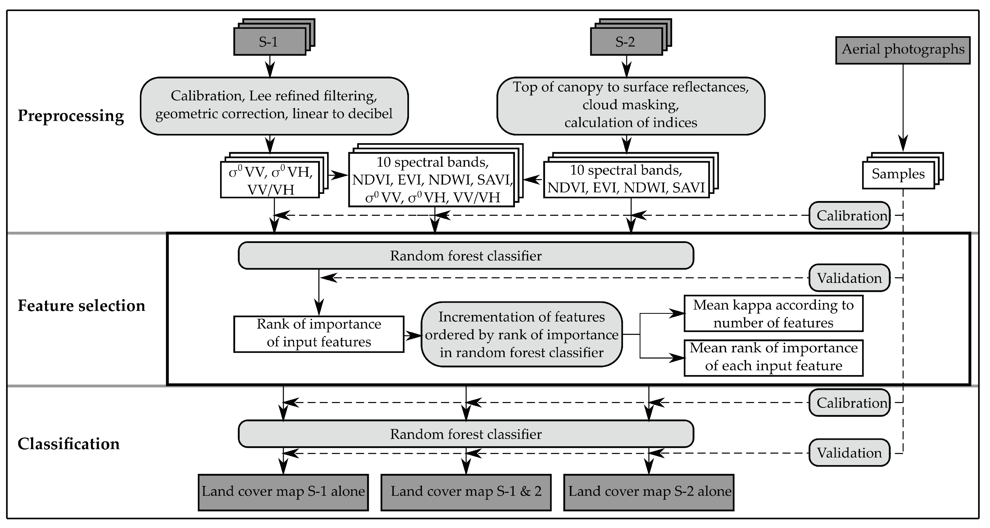
A set of 30 pairs of training and validation polygons were randomly selected from the reference polygons with a 50/50 ratio. The 30 random pairs were performed in order to obtain 30 trainings and 30 corresponding validations, allowing to compute average performances with confidence intervals [35]. The 50/50 ratio allows a more reliable comparison between training and validation samples than a ratio with a lower proportion of validation samples. For each set of selected training polygons, 300 and 1000 pixels per class were randomly selected for the Brazilian and Spanish study areas, respectively. The same random selection of pixels was applied to each set of associated validation polygons. This selection was performed to avoid over-representing large polygons at the expense of small polygons in the training and validation samples and to have the same number of samples for each class.

3.2. Preprocessing

The S-1 images were preprocessed using the Sentinel-1 Toolbox (Sentinel-1 toolbox, ESA, http://step.esa.int/main/toolboxes/sentinel-1-toolbox/). The images were first radiometrically calibrated to extract the backscattering coefficients ( σ 0 V V , σ 0 V H ) (Figure 2). A speckle filter was then applied (Lee refined, with a 7 × 7 window, [52]). The images were geo-coded using Shuttle Radar Topography Mission data to correct topographic deformations (geometric correction accuracy < 1 pixel) and were projected onto the ETRS89-TM3/ETRS0 system (EPSG 3042) and the WGS84/UTM 22S system (EPSG 32722) for the Spanish and the Brazilian study areas, respectively. A ratio channel was produced (VV/VH) from the backscattering coefficient images. All images were then converted from linear to decibel (dB).
Spectral bands and indices were derived from S-2 images. For the Brazilian study area, the Sen2Cor application (Sen2Cor, ESA, http://step.esa.int/main/third-party-plugins-2/sen2cor/) was used to transform L1C tiles to level L2A (TOC). Four vegetation indices commonly used in remote sensing were calculated for each S-2 mosaic for both study areas: EVI (Enhanced Vegetation Index), NDVI (Normalized Difference Vegetation Index), NDWI (Normalized Difference Water Index), and SAVI (Soil-adjusted Vegetation Index) (Table 3). Each mosaic was composed of 10 spectral bands and 4 vegetation indices.

3.3. Feature Selection and Classification

Incremental classification was performed using a random forest (RF) classifier. Two output analyses—mean rank of importance of each input feature and mean kappa index as a function of the number of features—were used to select the relevant features to use in the final classification. Incremental classification analyzes mapping quality as the type and number of features used are added, thus, determining at what combination and number of features the classification reaches an acceptable quality [35]. For each training and validation set (30 pairs), a RF algorithm was first applied to all of the features (dates and bands) to rank them in order of importance based on the mean decrease in the Gini index. Calle and Urea [57] demonstrated more robust results for exploring ranking stability using the mean decrease in the Gini index instead of the mean decrease in accuracy. The mean rank of importance of each feature was derived from the 30 ranks obtained from the 30 pairs of training and validation samples. We then ran as many RF algorithms as the number of features, starting with the two most important features and then adding the less important features until all of the features were processed. The kappa index was calculated for each classification to estimate the accuracy of the land cover classifications [58]. Rosenfield and Fitzpatrick-Lins [59] advised using the kappa index to measure classification accuracy.
We chose the RF algorithm [60] due to its advantages of having low sensitivity to feature selection, simple parameterization, and short calculation time [61,62]. We used it to select and classify features. In both cases, the number of trees was set to 100 to reduce calculation time sincePelletier et al. [63] demonstrated that it can be set to 100 without a major loss in accuracy. The experiments were performed using the randomForest package of R software (randomForest package version 4.6-14, Andy Liaw, https://cran.r-project.org/web/packages/randomForest/index.html). We used the OrfeoToolbox to calculate the final RF prediction (OrfeoToolbox version 6.6.1., CNES, https://www.orfeo-toolbox.org/).

3.4. Percentage of Pixels Confused

For both study areas, the features selected from analyses of S-1 data alone and S-2 data alone were used to calculate 30 RF classifiers. For each pair of classes, we calculated the percentage of confused pixels in relation to the total number of misclassified pixels. The following equation:
P c o n f P i x e l s p a i r s ( i , j ) = N b P i x e l s [ i , j ] + N b P i x e l [ j , i ] T o t a l P i x e l s ( P i x e l D i a g o n a l ) ,
where i and j are the classes in the pair, was applied to the 30 confusion matrices derived from the 30 RF classifications using the 30 pairs of training and validation samples. The mean of the percentages was calculated for each pair of classes. We then calculated the mean percentage of confused pixels per pair of classes in relation to the total number of misclassified pixels using the most important S-1 features and most important S-2 features.

3.5. Comparison of Classifications

We used McNemar’s X 2 test to analyze the significance of the difference or resemblance between the classifications derived from S-1 data alone vs. S-2 data alone, S-1 data alone vs. the combined S-1 and 2 data, and S-2 data alone vs. the combined S-1 and 2 data. This test, based on a binary 2 × 2 contingency matrix, shows the proportion of pixels correctly and incorrectly classified in two classification runs and allows the use of non-independent samples. A X 2 value lower than 3.14 means that the two classifications compared are non significantly different [64].

4. Results

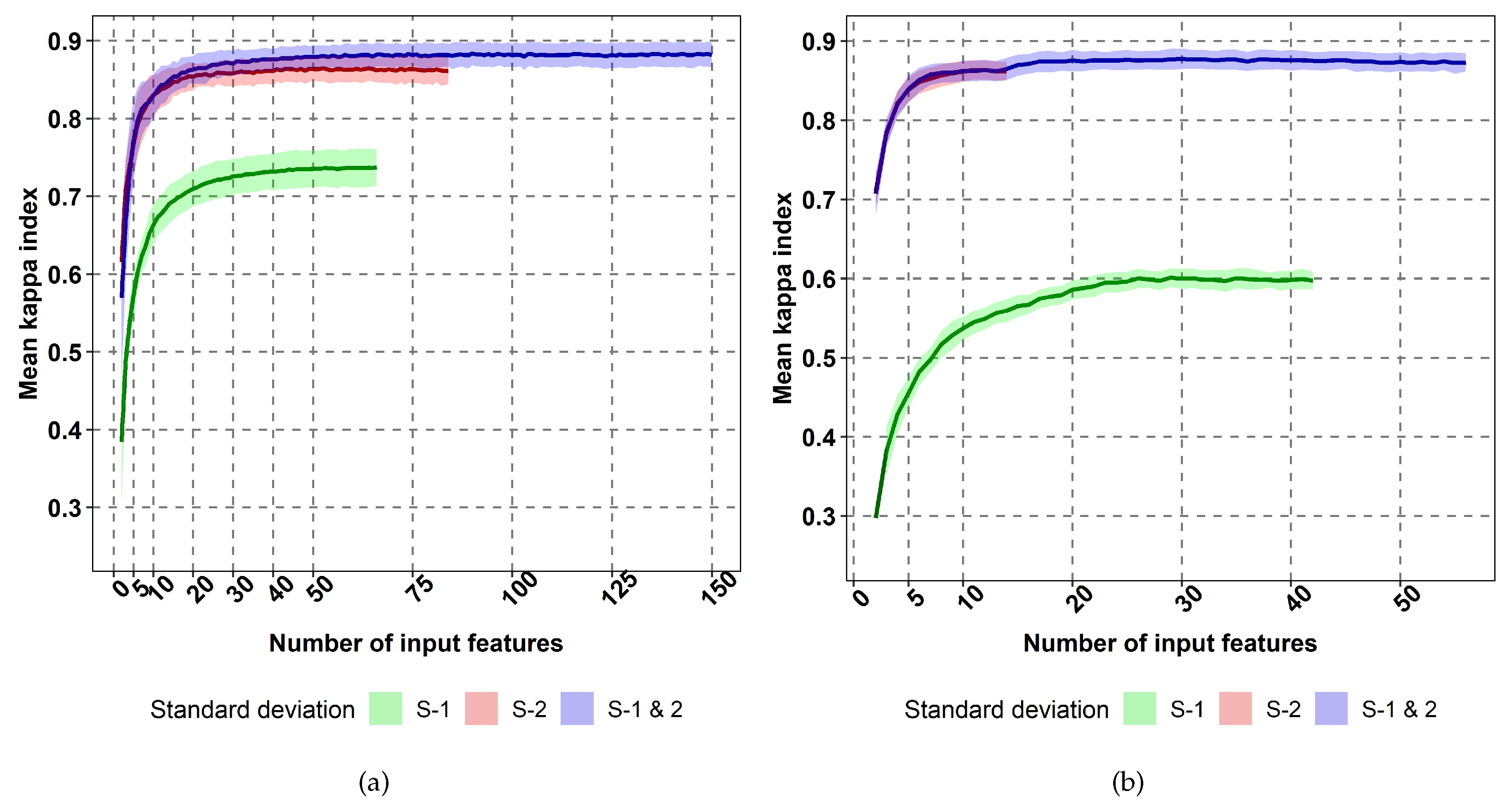
4.1. Contribution of Sentinel 1 & 2 Time Series to Map Land Cover

To estimate the contribution of the optical and SAR Sentinel time series, we analyzed the mean kappa index as a function of the number of input features. The combined use of S-1 and 2 data provided the best results for both study areas (Figure 3). However, for the standard deviation of the kappa index, results of the combined use of S-1 and 2 data were similar to those of S-2 data alone. The improvement in classification due to combining S-1 and 2 data rather than using S-2 data alone was perceptible up to 30 input features for the Spanish study area. For the Spanish study area, using the top ten S-2 features out of the 84 total S-2 features increased the mean kappa index by ca. 0.25 (i.e., from 0.58 to 0.83 ); the mean kappa index continued to increase slightly up to 40 input features and then stabilized. For the Brazilian study area, using the top 7 S-2 features out of the 14 total S-2 features increased the mean kappa index by ca. 0.15 (i.e., from 0.70 to 0.85); the mean kappa index continued to increase slightly up to 9 input features and then stabilized.
Using S-1 data alone yielded the lowest accuracy for both study sites. The mean kappa index was higher for the Spanish area than for the Brazilian area, as was the maximum kappa index (ca. 0.73 and 0.60, respectively). Compared to the mean kappa indices of S-2 data alone, those of S-1 data alone were lower by 0.08–0.20 for the Spanish study area and by 0.28–0.40 for the Brazilian study area.

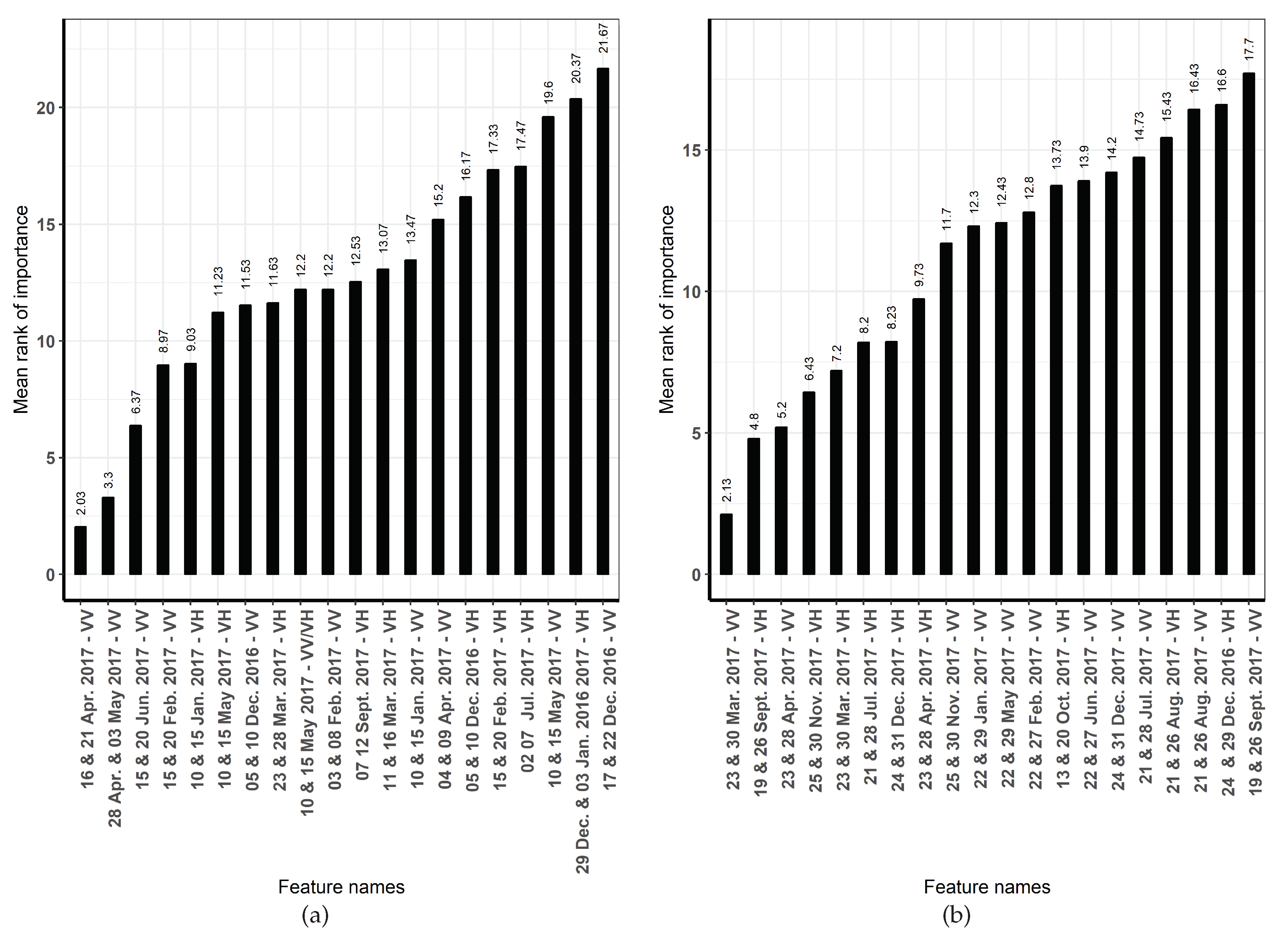
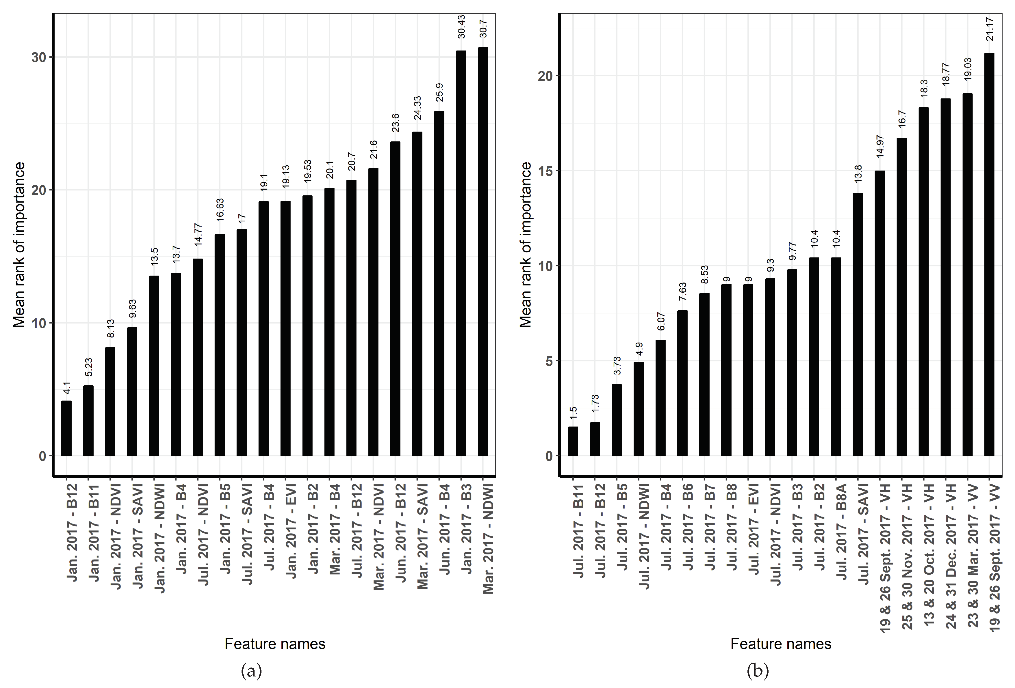
4.2. Importance of Input Features

When using S-2 data alone, bands 11 and 12 (the short-wave infrared (SWIR) domain) were the most important features for both study areas (mean rank of importance of 1.77 (B11) and 4.07 (B12), and of 1.43 (B12) and 1.63 (B11) for the Spanish and Brazilian study areas respectively) (Figure 4). For the Spanish area, the vegetation indices were relevant, with 11 of them among the top 20: 4 SAVI and 4 NDVI (1 each in January, March, June, and July), 2 NDWI (in January and March) and, although less relevant for classifying forest–agriculture mosaics, EVI. For the Brazilian study area, NDWI was the most relevant index (ranked 3rd), while other spectral bands were more relevant than EVI, NDVI, or SAVI.
When assessing the relevance of time periods using S-2 data alone (Figure 4a), January was the most important month for discriminating the 8 land cover classes, since it was the month of the top 6 features (mean rank of importance = 1.77–11). In addition, March and July appeared among the top ten features. The least important months were August and April.
When using S-1 data alone, the VV/VH ratio was not useful for mapping land cover in these two forest–agriculture mosaics. For both study areas, VV polarization was the most important feature. For the Spanish and Brazilian study areas, the VV mean ranks of importance were of 2.03 and 2.13, respectively (Figure 5). The top 20 features, however, had a nearly equal number of VV and VH features (10 VV and 9 VH polarization dates for the Spanish study area, 11 VV and 9 VH polarization dates for the Brazilian study area). When assessing the relevance of time periods using S-1 data alone, the months from December to May were relevant for the Spanish study area. In contrast, months from both dry and wet seasons were among the top ten features (January, March, April, July, September, November, December) for the Brazilian study area.
When combining S-1 and 2 data, the top 20 important features were all S-2 features for the Spanish study area and mostly S-2 features (the top 14) for the Brazilian study area (Figure 6).
As a trade-off between accuracy and processing time, we decided to maintain a minimum but sufficient number of features for classification (Table 4). In the following experiments, we choose to keep the 20 most important S-1 features and 10 S-2 features, and the 10 most important S-1 features and 7 S-2 features on the Spanish and Brazilian study areas, respectively (Table 4). Due to the large majority of S-2 features in the top 20 important features of combined S-1 and 2 data (Figure 6), we decided to combine the previously selected features of S-1 data alone and S-2 data alone to predict the land cover classes combining S-1 and 2 data (Table 4).

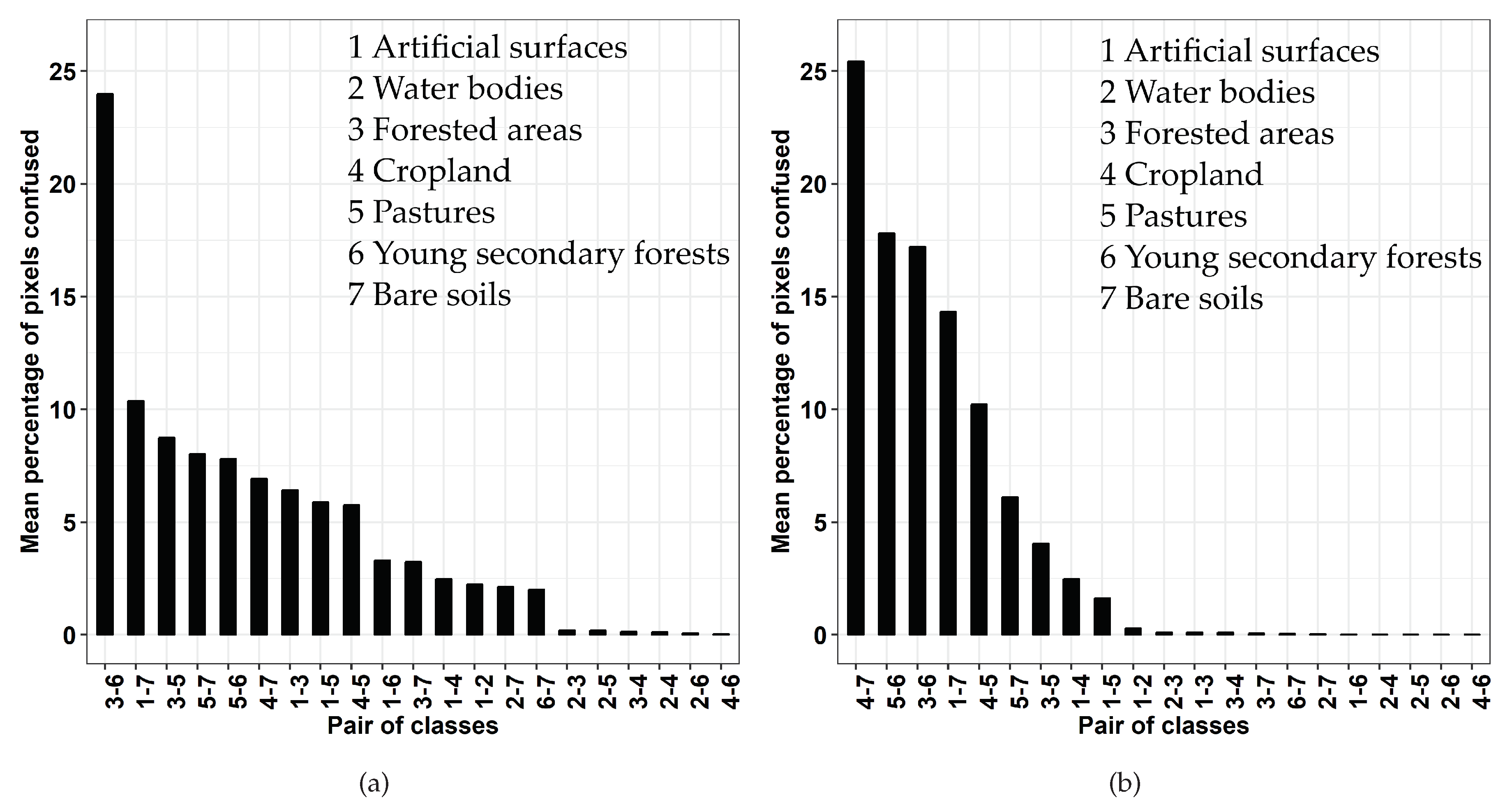
4.3. Confusion between Classes

Using the S-1 features for the Spanish study area, forested areas vs. shrublands, shrublands vs. permanent herbaceous vegetation, and bare soils vs. winter vegetation were the pairs of classes most often confused (Figure 7a). Using the S-2 features, bare soils vs. artificial surfaces, bare soils vs. winter vegetation, and forested areas vs. shrublands were the most confused pairs of classes (Figure 7b). Forested areas and shrublands were not well discriminated using S-1 or S2 features. Shrublands vs. permanent vegetation were better discriminated using S-2 data than S-1 data.
Using the S-1 features for the Brazilian study area, most forested areas and young secondary forests pair of classes was confused, unlike the other pairs of classes, including forested areas vs. pastures (Figure 8a). Using the S-2 features, cropland vs. bare soils, pastures vs. young secondary forests, and forested areas vs. young secondary forests were the most confused pairs of classes (Figure 8b). Forested areas vs. young secondary forests were better discriminated by S-2 than S-1 features. However, pastures and young secondary forests were better discriminated by S-1 than S-2 features. On both study areas, bare soils vs. artificial surfaces were discriminated better by S-1 data than S-2 data features.

4.4. Prediction of Selected Features

Misclassification errors in the land cover map of forest–agriculture mosaics of the Spanish study area—due to cloud confusions using S-2 data alone and slopes using S-1 data alone—were partly corrected using combined S-1 (Figure 9).
The combined S-1 and 2 classification of the Brazilian study area (Figure 10) was more accurate than classification by S-2 data alone. Misclassification of cropland, which was confused with artificial surfaces using S-2 data alone, was partly corrected with combined S-1 and 2 data.

4.5. McNemar χ 2 Test Results

According to McNemar’s χ 2 test, all land cover class predictions differed significantly ( χ 2 > 3.14), and S-2 data alone vs. combined S-1 and 2 data for the Brazilian study area is not significant (p-value = NS) (Table 5). Thus, we concluded that all classifications differed.

5. Discussion

5.1. Relative Contributions of S-1 and S-2 Data to Map Land Cover of Forest–Agriculture Mosaics

The land cover classes that comprise forest–agriculture mosaics are distributed along a landscape gradient, with transition classes such as shrublands to forest or pasture to young secondary forests, which result in misclassifications. S-1 data alone were least accurate for mapping land cover of forest–agriculture mosaics, with a best mean kappa index of 0.73, vs. 0.87 and 0.89 for S-2 data alone and combined S-1 and 2 data, respectively (Figure 3). For example, S-2 data discriminated forested areas from young secondary forests better than S-1 data for the Brazilian study area (Figure 8). This may be because SAR sensors are sensitive to vegetation structure, while optical sensors are sensitive to chlorophyll content. Thus, when observed at a 10m resolution, broad vegetation classes were discriminated more easily by their physiology than their physical structure. Also, VV and VH polarizations were the most important S-1 features for discriminating land cover classes, while the VV/VH ratio was not useful (Figure 5). While it is known that VH polarization is more sensitive to vegetation than VV polarization [65] (Patel et al., 2006), results show that both polarizations had an equivalent low contribution to classify forest–agriculture mosaics, as well as the ratio VV/VH. We can conclude that in this case the C-band of Sentinel-1 was not relevant to classify vegetation classes. In general, the C-band SAR is less suitable than L-Band for forest change monitoring due to a lower penetration depth and a rapid saturation of the signal [66]). For example, Patel et al. [65]) demonstrated that L-band is more sensitive to plant density than C-band, and that C-band interacts mostly with the primary branches of the canopy while L-band within the vegetation canopy. We used S-1 GRD products that record backscattering coefficients (VV and VH) because they require less processing time than Single Look Complex products, which preserve the phase information. However, using texture, coherence, and polarimetric indices derived from full-polar radar data, such as RADARSAT-2 data, could improve classification based on S-1 data alone [35,36,67,68,69,70]. Thus, although Bagdhadi et al. [71] concluded that using polarimetric indices (Shannon Entropy (SE) and span) derived from polSAR RADARSAT-2 images did not improve estimates of soil moisture and vegetation parameters, Betbeder et al. [72] demonstrated the greater utility of the SE index than backscattering coefficients for mapping wetland vegetation using dual-pol TerraSAR-X time series. The best mean kappa index achieved with S-1 data was higher for the Spanish study area than for the Brazilian study area (0.73 vs. 0.60, respectively) (Figure 3). This could be due to differences in the classification methods (different numbers of classes and land cover types) and to the number of S-1 images used to classify land cover types (22 dates for the Spanish study area vs. 14 dates for the Brazilian study area). For the Spanish study area, the classification results achieved using S-1 data alone show that misclassification errors are most often located on mountain slopes. These errors are due to the acquisition of SAR images in slant range geometry that causes layover and foreshortening effects [15]. Moreover, it is known that soil moisture and roughness influence the radar backscatter depending on frequency, polarization and the incidence angle of the incoming microwave. Holah et al. [73] found that the sensitivity to surface roughness is more important using HH and HV polarizations than VV polarization. However, Baghdadi et al. [74] demonstrated that the soil moisture was not very dependent on polarization. The effects of soil moisture on forest–agriculture classification are rather limited using C-band due to a low penetration depth of the microwaves compared to L-band [75], however C-band is more sensitive to roughness [76]. Lastly, the higher the incidence angle, the more important the sensitivity of the SAR to surface roughness [77].
However, S-1 data sometimes discriminated better than S-2 data—for bare soils and artificial surfaces—(Figure 7 and Figure 8) because the SAR signal reacts differently to these two land cover classes, with double-bounce on buildings and single-bounce on flat bare soils [15], while their spectral signatures in the optical domain are similar (high reflectance values in green, blue and red bands). When using S-2 data alone, SWIR bands were the most important features for discriminating land cover classes (Figure 4). The importance of S-2 SWIR bands has been demonstrated for mapping vegetation and forests [23,78]. Vegetation indices derived from S-2 data (e.g., SAVI, NDVI, NDWI) discriminated better than spectral bands for the Spanish study area, while NDWI was the most important vegetation index for the Brazilian study area. The sensitivity of the blue band to water contained in vegetation could explain why NDWI is well suited to tropical vegetation, while NDVI saturates at high biomass values [55,79]. The EVI, which was developed for MODIS, was a less important feature than other vegetation indices for both study areas. It could be interesting to calculate other vegetation indices that are used for crop discrimination such as S2REP (Sentinel-2 Red-Edge Position), IRECI (Inverted Red-Edge Chlorophyll Index), MTCI (MERIS Terrestrial Chlorophyll Index) or SRI (Simple Ratio Index) [80,81].
The best mean kappa index using combined S-1 and 2 data (0.88) did not differ greatly from that using S-2 data alone (0.86) (Figure 3). Thus, the use of S-2 data alone was sufficient to discriminate the land cover classes with high accuracy. However, the backscattering intensity from S-1 data alone provided additional relevant information, since predictions of land cover classes using S-1 data alone, S-2 data alone, and combined S-1 and 2 data differed according to McNemar’s χ 2 test (Table 5). For example, the misclassification between cropland and artificial surfaces for the Brazilian study area when using S-2 data alone was partly corrected using combined S-1 and 2 data (Figure 10).

5.2. Using S-1 and S-2 Data to Identify the Key Time Periods for Classifying Land Cover

Based on the classification results using S-1 data alone, S-2 data alone, and combined S-1 and 2 data, classification accuracy was strongly related to the number of dates. Classification accuracy increased when dates were added to the RF classifier (Figure 3, Figure 4a, Figure 5 and Figure 6). The relevance of high temporal resolution underlines the importance of describing and taking into account the phenology of vegetation to map forest–agriculture mosaics. For the Spanish study area, January, March, June, and July features are among the top 20 important S-2 features (Figure 4a). This may have been because the S-2 sensor is sensitive to chlorophyll content in vegetation, and these months are key periods of chlorophyll activity. The features of the months from December to May were among the top 20 S-1 features for this study area, while the summer period was not relevant (Figure 5a). This is probably because SAR sensors, which are sensitive to the internal structure of elements, penetrate vegetation better during the leaf-off period. Only one S-2 date was used for the Brazilian study area, which precluded studying the importance of time period. In addition, no clear time periods emerged from the importance ranks of the S-1 time series (Figure 5b). Thus, no intra-annual time period seems more important than others for S-1 time series for discriminating land cover types in Paragominas. Unlike the Cantabrian Range, where the seasons differ, temperatures and precipitation are relatively constant in Pará, with a drier season from July to October [82]. In addition, most of the dynamics of human practices in pastures, forested areas, and plantations are inter-annual rather than intra-annual [83].

5.3. The Robustness of the Method for Different Landscapes

The results show that the method can be applied to forest–agriculture mosaics in two landscapes with contrasting climates (i.e., tropical, temperate) and vegetation types (e.g., tropical forests, shrublands, coniferous and deciduous forests). S-1 and S-2 features were selected according to their respective importance in each study area, which highlighted relevant features and time periods for the two areas. Land cover maps of the two study areas were produced with a high degree of accuracy and a short processing time. Time series are used to map the land cover of forest–agriculture mosaics, but processing them requires high computational capacity. The method enabled focusing on specific time periods and features to reduce the time required for image processing.

6. Conclusions

An incremental procedure based on ranking the importance of the input features derived from S-1 and S-2 time series was used to discriminate land cover classes in forest–agriculture mosaics. The method automatically selected relevant features (spectral bands and/or vegetation indices) and time periods to classify land cover types in such landscapes. S-2 data alone were more relevant than S-1 data alone for mapping the land cover of forest–agriculture mosaics, and combining S-1 and 2 data slightly improved results compared to those of S-2 data alone. Using polarimetric indices, such as the SE index, which has already shown potential for characterizing vegetation, can improve predictions of S-1 data alone. Indeed, SAR data are useful in cloudy regions; the high cloud cover in the S-2 time series was the main source of misclassification errors.

Author Contributions

Conceptualization, A.M., L.H.-M., J.B. (Julie Betbeder) and J.B. (Jacques Baudry); Methodology, A.M., J.B. (Julie Betbeder) and L.H.-M.; Software, A.M., J.B. (Julie Betbeder) and G.C.; Validation, A.M., J.B. (Julie Betbeder), F.R., C.B., V.G. and L.B.; Resources, R.P.C., C.B., J.B. (Julie Betbeder), L.B., V.G., C.C. and M.M.; Data Curation, A.M., F.R., J.B. (Julie Betbeder) and C.B.; Writing-Original Draft Preparation, A.M.; Writing-Review & Editing, A.M., L.H.-M., J.B. (Julie Betbeder) and J.B. (Jacques Baudry); Visualization, A.M., L.H.-M., F.R. and C.B.; Supervision, J.B. (Julie Betbeder), L.H.-M., and J.B. (Jacques Baudry); Project Administration, L.H.-M.; Funding Acquisition, L.H.-M., J.B. (Julie Betbeder), J.B. (Jacques Baudry), V.G. and L.B.

Funding

This research was funded through the 2015-2016 BiodivERsA COFUND call for research proposals, with the national funders ANR, MINECO, and BELSPO. A. Mercier has a Ph.D. grant from MESRI (Ministry of Higher Education, Research and Innovation of France), PhD grant 2017. The study in Brazil was sponsored by the ODYSSEA Project “Observatory of the dynamics of interactions between societies and environment in the Amazon”, financed by the European Commission, Horizon 2020, and supported by the French Space Agency CNES and TOSCA (Terre, Océan, Surfaces continentales, Atmosphère) program CASTAFIOR project (Caractérisation et dynamique des Agro-écoSystèmes Tropicaux Amazoniens par Fusion d’Image Optique et Radar).

Acknowledgments

We thank Mickaël and Michelle Corson for English editing.

Conflicts of Interest

The authors declare no conflict of interest. The funders had no role in the design of the study; in collection, analysis, or interpretation of data; in writing the manuscript; or in the decision to publish the results.

References

  1. Gardner, T.A.; Ferreira, J.; Barlow, J.; Lees, A.C.; Parry, L.; Vieira, I.C.G.; Berenguer, E.; Abramovay, R.; Aleixo, A.; Andretti, C.; et al. A social and ecological assessment of tropical land uses at multiple scales: The Sustainable Amazon Network. Philos. Trans. R. Soc. B 2013, 368, 20130307. [Google Scholar] [CrossRef]
  2. Foley, J.A.; Ramankutty, N.; Brauman, K.A.; Cassidy, E.S.; Gerber, J.S.; Johnston, M.; Mueller, N.D.; O’Connell, C.; Ray, D.K.; West, P.C.; et al. Solutions for a cultivated planet. Nature 2011, 478, 337–342. [Google Scholar] [CrossRef] [Green Version]
  3. Altieri, M.A. The ecological role of biodiversity in agroecosystems. Agric. Ecosyst. Environ. 1999, 74, 19–31. [Google Scholar] [CrossRef] [Green Version]
  4. Krebs, J.R.; Wilson, J.D.; Bradbury, R.B.; Siriwardena, G.M. The second Silent Spring? Nature 1999, 400, 611–612. [Google Scholar] [CrossRef]
  5. Fahrig, L.; Baudry, J.; Brotons, L.; Burel, F.G.; Crist, T.O.; Fuller, R.J.; Sirami, C.; Siriwardena, G.M.; Martin, J.L. Functional landscape heterogeneity and animal biodiversity in agricultural landscapes. Ecol. Lett. 2011, 14, 101–112. [Google Scholar] [CrossRef]
  6. Billeter, R.; Liira, J.; Bailey, D.; Bugter, R.; Arens, P.; Augenstein, I.; Aviron, S.; Baudry, J.; Bukacek, R.; Burel, F.; et al. Indicators for biodiversity in agricultural landscapes: A pan-European study. J. Appl. Ecol. 2008, 45, 141–150. [Google Scholar] [CrossRef]
  7. Fahrig, L. Effects of Habitat Fragmentation on Biodiversity. Annu. Rev. Ecol. Evol. Syst. 2003, 34, 487–515. [Google Scholar] [CrossRef]
  8. Hanski, I. Habitat Loss, the Dynamics of Biodiversity, and a Perspective on Conservation. AMBIO 2011, 40, 248–255. [Google Scholar] [CrossRef] [PubMed] [Green Version]
  9. Zeller, K.A.; McGarigal, K.; Whiteley, A.R. Estimating landscape resistance to movement: A review. Landsc. Ecol. 2012, 27, 777–797. [Google Scholar] [CrossRef]
  10. Estes, L.; Chen, P.; Debats, S.; Evans, T.; Ferreira, S.; Kuemmerle, T.; Ragazzo, G.; Sheffield, J.; Wolf, A.; Wood, E.; et al. A large-area, spatially continuous assessment of land cover map error and its impact on downstream analyses. Glob. Chang. Biol. 2018, 24, 322–337. [Google Scholar] [CrossRef]
  11. Chen, B.; Huang, B.; Xu, B. Multi-source remotely sensed data fusion for improving land cover classification. ISPRS J. Photogramm. Remote Sens. 2017, 124, 27–39. [Google Scholar] [CrossRef]
  12. Aplin, P. Remote sensing: Land cover. Prog. Phys. Geogr. 2004, 28, 283–293. [Google Scholar] [CrossRef]
  13. Wulder, M.A.; Hall, R.J.; Coops, N.C.; Franklin, S.E. High Spatial Resolution Remotely Sensed Data for Ecosystem Characterization. BioScience 2004, 54, 511–521. [Google Scholar] [CrossRef]
  14. Gómez, C.; White, J.C.; Wulder, M.A. Optical remotely sensed time series data for land cover classification: A review. ISPRS J. Photogramm. Remote Sens. 2016, 116, 55–72. [Google Scholar] [CrossRef] [Green Version]
  15. Lee, J.S.; Pottier, E. Polarimetric Radar Imaging: From Basics to Applications, 1st ed.; CRC Press, Taylor & Francis Group: Boca Raton, FL, USA, 2009; ISBN 978-1420054972. [Google Scholar]
  16. Wiseman, G.; McNairn, H.; Homayouni, S.; Shang, J. RADARSAT-2 Polarimetric SAR Response to Crop Biomass for Agricultural Production Monitoring. IEEE J. Sel. Top. Appl. Earth Obs. Remote Sens. 2014, 7, 4461–4471. [Google Scholar] [CrossRef]
  17. Baghdadi, N.; Boyer, N.; Todoroff, P.; El Hajj, M.; Bégué, A. Potential of SAR sensors TerraSAR-X, ASAR/ENVISAT and PALSAR/ALOS for monitoring sugarcane crops on Reunion Island. Remote Sens. Environ. 2009, 113, 1724–1738. [Google Scholar] [CrossRef]
  18. Fieuzal, R.; Baup, F.; Marais-Sicre, C. Monitoring Wheat and Rapeseed by Using Synchronous Optical and Radar Satellite Data—From Temporal Signatures to Crop Parameters Estimation. Adv. Remote Sens. 2013, 2, 162–180. [Google Scholar] [CrossRef]
  19. McNairn, H.; Brisco, B. The application of C-band polarimetric SAR for agriculture: A review. Can. J. Remote Sens. 2004, 30, 525–542. [Google Scholar] [CrossRef]
  20. Álvarez Mozos, J.; Verhoest, N.E.C.; Larrañaga, A.; Casalí, J.; González-Audícana, M. Influence of Surface Roughness Spatial Variability and Temporal Dynamics on the Retrieval of Soil Moisture from SAR Observations. Sensors 2009, 9, 463–489. [Google Scholar] [CrossRef] [Green Version]
  21. Baup, F.; Mougin, E.; de Rosnay, P.; Timouk, F.; Chênerie, I. Surface soil moisture estimation over the AMMA Sahelian site in Mali using ENVISAT/ASAR data. Remote Sens. Environ. 2007, 109, 473–481. [Google Scholar] [CrossRef] [Green Version]
  22. Joshi, N.; Baumann, M.; Ehammer, A.; Fensholt, R.; Grogan, K.; Hostert, P.; Jepsen, M.R.; Kuemmerle, T.; Meyfroidt, P.; Mitchard, E.T.A.; et al. A Review of the Application of Optical and Radar Remote Sensing Data Fusion to Land Use Mapping and Monitoring. Remote Sens. 2016, 8, 70. [Google Scholar] [CrossRef]
  23. Immitzer, M.; Vuolo, F.; Atzberger, C. First Experience with Sentinel-2 Data for Crop and Tree Species Classifications in Central Europe. Remote Sens. 2016, 8, 166. [Google Scholar] [CrossRef]
  24. Clark, M.L. Comparison of simulated hyperspectral HyspIRI and multispectral Landsat 8 and Sentinel-2 imagery for multi-seasonal, regional land-cover mapping. Remote Sens. Environ. 2017, 200, 311–325. [Google Scholar] [CrossRef]
  25. Colkesen, I.; Kavzoglu, T. Ensemble-based canonical correlation forest (CCF) for land use and land cover classification using sentinel-2 and Landsat OLI imagery. Remote Sens. Lett. 2017, 8, 1082–1091. [Google Scholar] [CrossRef]
  26. Mongus, D.; Žalik, B. Segmentation schema for enhancing land cover identification: A case study using Sentinel 2 data. Int. J. Appl. Earth Obs. Géoinf. 2018, 66, 56–68. [Google Scholar] [CrossRef]
  27. Haas, J.; Ban, Y. Urban Land Cover and Ecosystem Service Changes based on Sentinel-2A MSI and Landsat TM Data. IEEE J. Sel. Top. Appl. Earth Obs. Remote Sens. 2018, 11, 485–497. [Google Scholar] [CrossRef]
  28. Belgiu, M.; Csillik, O. Sentinel-2 cropland mapping using pixel-based and object-based time-weighted dynamic time warping analysis. Remote Sens. Environ. 2018, 204, 509–523. [Google Scholar] [CrossRef]
  29. Csillik, O.; Belgiu, M. Cropland mapping from Sentinel-2 time series data using object-based image analysis. In Proceedings of the 20th AGILE International Conference on Geographic Information Science Societal Geo-Innovation Celebrating 20 years of GIS Research, Wageningen, The Netherlands, 9–12 May 2017. [Google Scholar]
  30. Defourny, P.; Bontemps, S.; Bellemans, N.; Cara, C.; Dedieu, G.; Guzzonato, E.; Hagolle, O.; Inglada, J.; Nicola, L.; Rabaute, T.; et al. Near real-time agriculture monitoring at national scale at parcel resolution: Performance assessment of the Sen2-Agri automated system in various cropping systems around the world. Remote Sens. Environ. 2019, 221, 551–568. [Google Scholar] [CrossRef]
  31. Lambert, M.J.; Traoré, P.C.S.; Blaes, X.; Baret, P.; Defourny, P. Estimating smallholder crops production at village level from Sentinel-2 time series in Mali’s cotton belt. Remote Sens. Environ. 2018, 216, 647–657. [Google Scholar] [CrossRef]
  32. Wu, M.; Yang, C.; Song, X.; Hoffmann, W.C.; Huang, W.; Niu, Z.; Wang, C.; Li, W.; Yu, B. Monitoring cotton root rot by synthetic Sentinel-2 NDVI time series using improved spatial and temporal data fusion. Sci. Rep. 2018, 8, 2016. [Google Scholar] [CrossRef] [Green Version]
  33. Jönsson, P.; Cai, Z.; Melaas, E.; Friedl, M.A.; Eklundh, L. A Method for Robust Estimation of Vegetation Seasonality from Landsat and Sentinel-2 Time Series Data. Remote Sens. 2018, 10, 635. [Google Scholar] [CrossRef]
  34. Puletti, N.; Chianucci, F.; Castaldi, C. Use of Sentinel-2 for forest classification in Mediterranean environments. Ann. Silvic. Res. 2017. [Google Scholar] [CrossRef]
  35. Inglada, J.; Vincent, A.; Arias, M.; Marais-Sicre, C. Improved Early Crop Type Identification By Joint Use of High Temporal Resolution SAR And Optical Image Time Series. Remote Sens. 2016, 8, 362. [Google Scholar] [CrossRef]
  36. Zhou, T.; Zhao, M.; Sun, C.; Pan, J. Exploring the Impact of Seasonality on Urban Land-Cover Mapping Using Multi-Season Sentinel-1A and GF-1 WFV Images in a Subtropical Monsoon-Climate Region. ISPRS J. Photogramm. Remote Sens. 2017, 7, 3. [Google Scholar] [CrossRef]
  37. Kussul, N.; Lavreniuk, M.; Skakun, S.; Shelestov, A. Deep Learning Classification of Land Cover and Crop Types Using Remote Sensing Data. IEEE Trans. Geosci. Remote Sens. Lett. 2017, 14, 778–782. [Google Scholar] [CrossRef]
  38. Reiche, J.; Hamunyela, E.; Verbesselt, J.; Hoekman, D.; Herold, M. Improving near-real time deforestation monitoring in tropical dry forests by combining dense Sentinel-1 time series with Landsat and ALOS-2 PALSAR-2. Remote Sens. Environ. 2018, 204, 147–161. [Google Scholar] [CrossRef]
  39. Laurin, G.V.; Balling, J.; Corona, P.; Mattioli, W.; Papale, D.; Puletti, N.; Rizzo, M.; Truckenbrodt, J.; Urban, M. Above-ground biomass prediction by Sentinel-1 multitemporal data in central Italy with integration of ALOS2 and Sentinel-2 data. J. Appl. Remote Sens. 2018, 12, 016008. [Google Scholar] [CrossRef]
  40. García, D.; Quevedo, M.; Obeso, J.R.; Abajo, A. Fragmentation patterns and protection of montane forest in the Cantabrian range (NW Spain). For. Ecol. Manage. 2005, 208, 29–43. [Google Scholar] [CrossRef]
  41. Gastón, A.; Ciudad, C.; Mateo-Sánchez, M.C.; García-Viñas, J.I.; López-Leiva, C.; Fernández-Landa, A.; Marchamalo, M.; Cuevas, J.; de la Fuente, B.; Fortin, M.J.; et al. Species’ habitat use inferred from environmental variables at multiple scales: How much we gain from high-resolution vegetation data? Int. J. Appl. Earth Obs. Géoinf. 2017, 55, 1–8. [Google Scholar] [CrossRef]
  42. Mateo-Sánchez, M.C.; Gastón, A.; Ciudad, C.; García-Viñas, J.I.; Cuevas, J.; López-Leiva, C.; Fernández-Landa, A.; Algeet-Abarquero, N.; Marchamalo, M.; Fortin, M.J.; et al. Seasonal and temporal changes in species use of the landscape: How do they impact the inferences from multi-scale habitat modeling? Landsc. Ecol. 2016, 31, 1261–1276. [Google Scholar] [CrossRef]
  43. AQUASTAT—FAO’s Information System on Water and Agriculture. Available online: http://www.fao.org/nr/water/aquastat/irrigationmap/ESP/index.stm (accessed on 13 April 2019).
  44. Quevedo, M.; Bañuelos, M.J.; Obeso, J.R. The decline of Cantabrian capercaillie: How much does habitat configuration matter? Biol. Conserv. 2006, 127, 190–200. [Google Scholar] [CrossRef]
  45. Tritsch, I.; Sist, P.; Narvaes, I.d.S.; Mazzei, L.; Blanc, L.; Bourgoin, C.; Cornu, G.; Gond, V. Multiple Patterns of Forest Disturbance and Logging Shape Forest Landscapes in Paragominas, Brazil. Forests 2016, 7, 315. [Google Scholar] [CrossRef]
  46. Bourgoin, C.; Blanc, L.; Bailly, J.S.; Cornu, G.; Berenguer, E.; Oszwald, J.; Tritsch, I.; Laurent, F.; Hasan, A.; Sist, P.; et al. The Potential of Multisource Remote Sensing for Mapping the Biomass of a Degraded Amazonian Forest. Forests 2018, 9, 303. [Google Scholar] [CrossRef]
  47. Barlow, J.; Lennox, G.D.; Ferreira, J.; Berenguer, E.; Lees, A.C.; Nally, R.M.; Thomson, J.R.; Ferraz, S.F.d.B.; Louzada, J.; Oliveira, V.H.F.; et al. Anthropogenic disturbance in tropical forests can double biodiversity loss from deforestation. Nature 2016, 535, 144–147. [Google Scholar] [CrossRef] [Green Version]
  48. Viana, C.; Coudel, E.; Barlow, J.; Ferreira, J.; Gardner, T.; Parry, L. From red to green: Achieving an environmental pact at the municipal level in paragominas (Pará, Brazilian Amazon). 2012. Available online: http://agritrop-prod.cirad.fr/567220/1/document_567220.pdf (accessed on 8 October 2018).
  49. MAPAMA-Ministerio de Agricultura y Pesca, Alimentación y Medio Ambiente. Mapa Forestal de España a Escala 1:50,000. Available online: http://www.mapama.gob.es/es/biodiversidad/servicios/bancodatos-naturaleza/informacion-disponible/mfe50.aspx (accessed on 3 August 2018).
  50. User Guides—Sentinel-1 SAR—Level-1 Ground Range Detected—Sentinel Online. Available online: https://sentinel.esa.int/web/sentinel/user-guides/sentinel-1-sar (accessed on 7 March 2019).
  51. User Guides—Sentinel-2 MSI—Sentinel Online. Available online: https://sentinel.esa.int/web/sentinel/user-guides/sentinel-2-msi (accessed on 7 March 2019).
  52. Lee, J.S.; Jurkevich, L.; Dewaele, P.; Wambacq, P.; Oosterlinck, A. Speckle filtering of synthetic aperture radar images: A review. Remote Sens. Rev. 1994, 8, 255–267. [Google Scholar] [CrossRef]
  53. Rouse, J.W.J.; Haas, R.H.; Schell, J.A.; Deering, D.W. Monitoring vegetation systems in the Great Plains with ERTS. In Proceedings of the 3rd ERTS Symposium, Washington, DC, USA, 10–14 December 1973. [Google Scholar]
  54. Gao, B.C. NDWI—A normalized difference water index for remote sensing of vegetation liquid water from space. Remote Sens. Environ. 1996, 58, 257–266. [Google Scholar] [CrossRef]
  55. Huete, A.; Didan, K.; Miura, T.; Rodriguez, E.P.; Gao, X.; Ferreira, L.G. Overview of the radiometric and biophysical performance of the MODIS vegetation indices. Remote Sens. Environ. 2002, 83, 195–213. [Google Scholar] [CrossRef]
  56. Huete, A.R. A soil-adjusted vegetation index (SAVI). Remote Sens. Environ. 1988, 25, 295–309. [Google Scholar] [CrossRef]
  57. Calle, M.L.; Urrea, V. Letter to the Editor: Stability of Random Forest importance measures. Brief. Bioinform. 2011, 12, 86–89. [Google Scholar] [CrossRef]
  58. Cohen, J. A Coefficient of Agreement for Nominal Scales, A Coefficient of Agreement for Nominal Scales. Educ. Psychol. Meas. 1960, 20, 37–46. [Google Scholar] [CrossRef]
  59. Rosenfield, G.; Fitzpatrick-Lins, K. A coefficient of agreement as a measure of thematic classification accuracy. Photogramm. Eng. Remote Sens. 1986, 52, 5. [Google Scholar]
  60. Breiman, L. Random Forests. Mach. Learn. 2001, 45, 5–32. [Google Scholar] [CrossRef] [Green Version]
  61. Belgiu, M.; Drăguţ, L. Random forest in remote sensing: A review of applications and future directions. ISPRS J. Photogramm. Remote Sens. 2016, 114, 24–31. [Google Scholar] [CrossRef]
  62. Pelletier, C.; Valero, S.; Inglada, J.; Champion, N.; Marais Sicre, C.; Dedieu, G. Effect of Training Class Label Noise on Classification Performances for Land Cover Mapping with Satellite Image Time Series. Remote Sens. 2017, 9, 173. [Google Scholar] [CrossRef]
  63. Pelletier, C.; Valero, S.; Inglada, J.; Champion, N.; Dedieu, G. Assessing the robustness of Random Forests to map land cover with high resolution satellite image time series over large areas. Remote Sens. Environ. 2016, 187, 156–168. [Google Scholar] [CrossRef]
  64. Foody, G.M. Thematic map comparison. Photogramm. Eng. Remote Sens. 2004, 70, 627–633. [Google Scholar] [CrossRef]
  65. Patel, P.; Srivastava, H.S.; Panigrahy, S.; Parihar, J.S. Comparative evaluation of the sensitivity of multi-polarized multi-frequency SAR backscatter to plant density. Int. J. Remote Sens. 2006, 27, 293–305. [Google Scholar] [CrossRef]
  66. Woodhouse, I.H. Introduction to Microwave Remote Sensing; CRC Press: Boca Raton, FL, USA, 2017. [Google Scholar]
  67. Ranson, K.J.; Sun, G.; Kharuk, V.I.; Kovacs, K. Characterization of Forests in Western Sayani Mountains, Siberia from SIR-C SAR Data. Remote Sens. Environ. 2001, 75, 188–200. [Google Scholar] [CrossRef]
  68. Sonobe, R.; Tani, H.; Wang, X.; Kobayashi, N.; Shimamura, H. Discrimination of crop types with TerraSAR-X-derived information. Phys. Chem. Earth Parts A/B/C 2015, 83–84, 2–13. [Google Scholar] [CrossRef]
  69. Roychowdhury, K. Comparison between Spectral, Spatial and Polarimetric Classification of Urban and Periurban Landcover Using Temporal Sentinel-1 Images. In Proceedings of the XXIII ISPRS Congress, Prague, Czech Republic, 12–19 July 2016; pp. 789–796. [Google Scholar]
  70. Du, Z.; Ge, L.; Ng, A.H.M.; Zhu, Q.; Yang, X.; Li, L. Correlating the subsidence pattern and land use in Bandung, Indonesia with both Sentinel-1/2 and ALOS-2 satellite images. Int. J. Appl. Earth Obs. Géoinf. 2018, 67, 54–68. [Google Scholar] [CrossRef]
  71. Baghdadi, N.; El Hajj, M.; Zribi, M.; Fayad, I. Coupling SAR C-band and optical data for soil moisture and leaf area index retrieval over irrigated grasslands. IEEE J. Sel. Top. Appl. Earth Obs. Remote Sens. 2016, 9, 1129–1244. [Google Scholar] [CrossRef]
  72. Betbeder, J.; Rapinel, S.; Corpetti, T.; Pottier, E.; Corgne, S.; Hubert-Moy, L. Multitemporal classification of TerraSAR-X data for wetland vegetation mapping. J. Appl. Remote Sens. 2014, 8, 083648. [Google Scholar] [CrossRef]
  73. Holah, N.; Baghdadi, N.; Zribi, M.; Bruand, A.; King, C. Potential of ASAR/ENVISAT for the characterization of soil surface parameters over bare agricultural fields. Remote Sens. Environ. 2005, 96, 78–86. [Google Scholar] [CrossRef] [Green Version]
  74. Baghdadi, N.; Cerdan, O.; Zribi, M.; Auzet, V.; Darboux, F.; El Hajj, M.; Kheir, R.B. Operational performance of current synthetic aperture radar sensors in mapping soil surface characteristics in agricultural environments: application to hydrological and erosion modelling. Hydrol. Proc. 2008, 22, 9–20. [Google Scholar] [CrossRef]
  75. Ulaby, F.T.; Dubois, P.C.; Van Zyl, J. Radar mapping of surface soil moisture. J. Hydrol. 1996, 184, 57–84. [Google Scholar] [CrossRef]
  76. Mattia, F.; Le Toan, T.; Souyris, J.C.; De Carolis, C.; Floury, N.; Posa, F.; Pasquariello, N. The effect of surface roughness on multifrequency polarimetric SAR data. IEEE Trans. Geosci. Remote Sens. 1997, 35, 954–966. [Google Scholar] [CrossRef]
  77. Fung, A.; Chen, K. Dependence of the surface backscattering coefficients on roughness, frequency and polarization states. Int. J. Remote Sens 1992, 13, 1663–1680. [Google Scholar] [CrossRef]
  78. Chrysafis, I.; Mallinis, G.; Siachalou, S.; Patias, P. Assessing the relationships between growing stock volume and Sentinel-2 imagery in a Mediterranean forest ecosystem. Remote Sens. Lett. 2017, 8, 508–517. [Google Scholar] [CrossRef]
  79. Jackson, T.J.; Chen, D.; Cosh, M.; Li, F.; Anderson, M.; Walthall, C.; Doriaswamy, P.; Hunt, E.R. Vegetation water content mapping using Landsat data derived normalized difference water index for corn and soybeans. Remote Sens. Environ. 2004, 92, 475–482. [Google Scholar] [CrossRef]
  80. Frampton, W.J.; Dash, J.; Watmough, G.; Milton, E.J. Evaluating the capabilities of Sentinel-2 for quantitative estimation of biophysical variables in vegetation. ISPRS J. Photogramm. Remote Sens. 2013, 82, 83–92. [Google Scholar] [CrossRef] [Green Version]
  81. Jordan, C.F. Derivation of leaf-area index from quality of light on the forest floor. Ecology 1969, 50, 663–666. [Google Scholar] [CrossRef]
  82. World Weather Online, Para Monthly Climate Averages. Available online: https://www.worldweatheronline.com/para-weather/para/br.aspx (accessed on 17 August 2018).
  83. Piketty, M.G.; Poccard-Chapuis, R.; Drigo, I.; Coudel, E.; Plassin, S.; Laurent, F.; Thâles, M. Multi-level Governance of Land Use Changes in the Brazilian Amazon: Lessons from Paragominas, State of Pará. Forests 2015, 6, 1516–1536. [Google Scholar] [CrossRef] [Green Version]
Figure 1. Location of (a) the Spanish study area (© EuroGeographics for the country boundaries) and (b) the Brazilian study area (© 2018 GADM for the state boundaries).
Remotesensing 11 00979 g001
Figure 2. Flowchart of the image processing procedure. NIR = Near-infrared band. NDVI =Normalized difference vegetation index, EVI = Enhanced vegetation index, NDWI = Difference Water Index, SAVI = Soil adjusted vegetation index.
Remotesensing 11 00979 g002
Figure 3. Mean kappa index of the incremental classifications for Sentinel-1 data alone (green), Sentinel-2 data alone (red), and combined Sentinel-1 & 2 data (blue) as a function of the number of input features for (a) the Spanish study area and (b) the Brazilian study area.
Remotesensing 11 00979 g003
Figure 4. Mean rank of importance of the most important features for Sentinel-2 data alone for (a) the Spanish study area and (b) the Brazilian study area.
Remotesensing 11 00979 g004
Figure 5. Mean rank of importance of the most important features for Sentinel-1 data alone for (a) the Spanish study area and (b) the Brazilian study area.
Remotesensing 11 00979 g005
Figure 6. Mean rank of importance of the most important features for the combined use of Sentinel-1 and 2 data for (a) the Spanish study area and (b) the Brazilian study area.
Remotesensing 11 00979 g006
Figure 7. Mean percentage of pixels confused per pair of classes in relation to the total number of misclassified pixels using (a) the top 20 Sentinel-1 features and (b) the top ten Sentinel-2 features of the Spanish study.
Remotesensing 11 00979 g007
Figure 8. Mean percentage of pixels confused per pair of classes in relation to the total number of misclassified pixels using (a) the top ten Sentinel-1 features area and (b) the top 7 Sentinel-2 features of the Brazilian study area.
Remotesensing 11 00979 g008
Figure 9. Classification of the Spanish study area using combined Sentinel-1 & 2 data.
Remotesensing 11 00979 g009
Figure 10. Classification of the Brazilian study area using combined Sentinel-1 and 2 data.
Remotesensing 11 00979 g010
Table 1. Main characteristics of Sentinel-1A L1C images [50].
BandC (center frequency of 5.405 GHz)
ModeInterferometric Wide Swath
Product typeGround Range Detected
Pixel resolution20 × 22 m (range × azimuth)
Pixel spacing10 × 10 m (range × azimuth)
Temporal resolution5 days (Spain) and 12 days (Brazil)
OrbitAscending
PolarizationVV & VH
Swath250 × 350 km
Incidence angle (°)30.6–46.0
Table 2. Main characteristics of Sentinel-2 L1C/ L2A images [51].
Spatial and spectral resolutions10 × 10 m
B2 (490 nm), B3 (560 nm), B4 (665 nm) and B8 (842 nm)
20 × 20 m
B5 (705 nm), B6 (740 nm), B7 (783 nm), B8a (865 nm), B11 (1610 nm) and B12 (2190 nm)
Temporal resolution5 days
Swath width290 km
Tile size100 × 100 km
Table 3. Vegetation indices calculated from Sentinel-2 images for the Spanish study area. B= Blue band, G = Green band, R = Red band, NIR = Near-infrared band. NDVI = Normalized difference vegetation index, NDWI = Normalized difference water index, EVI = Enhanced vegetation index, SAVI = Soil adjusted vegetation index.
Vegetation IndexFormulaS-2 Band UsedOriginal Author
NDVI(NIR − R)/(NIR + R)(B8 − B4)/(B8 + B4)[53]
NDWI(NIR − G)/(NIR + G)(B8 − B3)/(B8 + B3)[54]
EVI2.5*(NIR − R)/(NIR + 6*R − 7.5*B) + 1)2.5*(B8 − B4)/(B8 + 6*R − 7.5*B2) + 1)[55]
SAVI(NIR − R)*1.5/(NIR + R + 0.5)(B8 − B4)*1.5/(B8 + B4 + 0.5)[56]
Table 4. Number of top important features selected for predictions for the Spanish and Brazilian case studies.
Type of DataSpainBrazil
S-1 alone2010
S-2 alone107
Table 5. McNemar’s χ 2 test results for the Spanish and Brazilian case studies. The χ 2 value less than 3.14 indicates that the two classifications were not significantly different.
Classifications ComparedSpainBrazil
χ 2 p-Value χ 2 p-Value
S-1 data alone vs. S-2 data alone113.23<0.0001368.47<0.0001
S-1 data alone vs. S-1 and 2379.82<0.0001439.00<0.0001
S-2 data alone vs. S-1 and 2105.39<0.0001 NS

