Remote Sensing of Pigment Content at a Leaf Scale: Comparison among Some Specular Removal and Specular Resistance Methods


1
Institute of Applied Remote Sensing and Information Technology, Zhejiang University, Hangzhou 310058, China
2
Key Laboratory of Agricultural Remote Sensing and Information System, Zhejiang Province, Zhejiang University, Hangzhou 310058, China
3
Key Laboratory of Environment Remediation and Ecological Health, Ministry of Education, College of Natural Resources and Environmental Science, Zhejiang University, Hangzhou 310058, China
*
Author to whom correspondence should be addressed.
Remote Sens. 2019, 11(8), 983; https://0-doi-org.brum.beds.ac.uk/10.3390/rs11080983
Submission received: 25 January 2019
/
Revised: 22 April 2019
/
Accepted: 22 April 2019
/
Published: 24 April 2019
(This article belongs to the Section Remote Sensing in Agriculture and Vegetation)
Abstract
:Leaf pigment content retrieval is negatively affected by specular reflectance. To alleviate this effect, some specific techniques that take specular reflectance or specular effects into account have been proposed. In this study, continuous wavelet transform (CWT) and specific techniques including some vegetation indices (VIs), radiative transfer (RT), and hybrid models, were examined and compared in the nadir and near the mirror-like direction, with a 30° incident zenith angle. Results show that the RT and hybrid models appeared to be ill-posed, and they were not applicable at this high-incident zenith angle (>20°). Most VIs effectively alleviated the specular disturbance in the forward 35° direction, and comparable accuracy was obtained between the two viewing directions. Multiple linear regression (MLR), derivative transformation, and CWT were effective for specular interference alleviation. The MLR-based methods (reflectance, derivatives, etc., as the independent variables and pigment content as the response) generally obtained higher retrieval accuracies than the VIs. With MLR-based methods, the retrieval was more accurate for chlorophylls than for carotenoids. CWT plus MLR (MLR on wavelet coefficients) was the most prominent among all the methods, and it generally obtained the highest accuracy. The results are 2.68 and 0.88 μg/cm2 for chlorophylls and carotenoids, respectively, in the nadir direction, and 2.42 and 0.86 μg/cm2 in the forward 35° direction, with reflectance or the first derivative input for CWT. In the retrieval, wavelet coefficients at the optimal decomposition scale may achieve a balance in corresponding to fine, and broad absorption features, and the overall reflectance properties.
1. Introduction
Leaf chlorophylls and carotenoids are of great importance for green plants. Chlorophylls play a crucial role in photosynthesis, which directly determines plant productivity [1,2]. With a close link to the nitrogen content, chlorophylls can be used as an indirect indicator for estimating plant nitrogen nutritional status [1]. Carotenoids absorb light and contribute energy for photosynthesis, and they can protect the photosynthetic system by dissipating excessive light energy received by the plant [3]. Moreover, the contents of the two pigments reveal various aspects of plant physiology and stress (e.g., nutrient deficiency) [4]. Given this, an estimation of pigment content is meaningful for many applications, such as agricultural management and ecological conservation.
One method to measure pigment content is through remote sensing. Compared to conventional wet chemistry, this method is fast, and time- and labor-saving. It does not destroy leaves, and thus can be used to monitor pigment status during the whole life-cycle of leaves. Via platforms such as satellites, remote sensing can be applied at spatial scales (e.g., [5]). The remote sensing of pigment content is mainly conducted based on empirical and physical approaches. The empirical approaches consist of classic vegetation indices (VIs) (e.g., [6]), multiple regression (e.g., [7]), machine learning algorithms (e.g., [8]), etc. These empirical approaches are data-driven, and they are established empirically, depending on the variability and quality of the data [9]. The physical approaches utilize some radiative transfer (RT) models, such as PROSPECT [10]. These models simulate leaf reflectance and transmittance, with some input parameters in the forward mode, while, in the reverse mode, the parameters are retrieved. The accuracies of these approaches depend on how well the scattering processes of the leaf are understood and how they are accounted for in models [11].
Of these remote sensing approaches, the reflectance data are the major data sources in application, and reflectance is usually used as a whole in retrieval. Nevertheless, leaf reflectance is composed of specular and diffuse components [12,13], and the two components are quite distinct. Specular reflectance occurs at the air-leaf cuticle interface. The incident radiation that generates the specular component is directly reflected, and it does not penetrate the leaf interior to interact with biochemical constituents such as pigments [14]. This component depends on the leaf surface biophysical properties, and has an angular distribution. Its spectral variability is not or very little affected by leaf biochemistry [13]. In contrast, the incident radiation that generates the diffuse component penetrates the leaf mesophyll, where multiple scattering and absorption by biochemical constituents (e.g., pigments and protein) occur. Diffuse component depends on biochemical concentrations, and it is isotropic in all directions. Its spectral variability is strongly related to leaf biochemistry [13]. Therefore, it is the diffuse component rather than the specular component that carries information about leaf biochemistry. Thus, as for pigment content retrieval, the existence of specular reflectance usually causes interference [15].
To reduce the disturbance from specular reflectance in remote sensing applications, many techniques have been proposed. These techniques may be divided into the specular removal and specular resistance types. The specular removal type explicitly estimates (accurately or roughly) the specular reflectance or the specular effect, and then separates them out from the reflectance. However, the specular resistance type does not make such estimations, and only develops approaches to reduce the probable specular effect. With respect to the first type, Rondeaux and Vanderbilt [16] calculated the specular reflectance based on polarized measurements, and built the specularly modified VIs to estimate plant photosynthetic activity. Sims and Gamon [17] used the reflectance at 445 nm as an approximation of specular reflectance, and this was subtracted to build the modified simple ratio (mSR705) and modified normalized difference (mND705) indices to retrieve leaf pigments. Jay et al. [18] developed the physically-based model COSINE to estimate the specular effect in the bidirectional reflectance factor (BRF), and coupled the simplified COSINE with PROSPECT (PROCOSINE) to retrieve foliar biochemistry. In PROCOSINE, the specular effect is represented by a term, and this can be retrieved. Li et al. [15] estimated the leaf specular reflectance through polarization measurements and subtracted this component to build diffuse reflectance-based VIs. With respect to the second technique type, based on a simple model [19], Peñuelas et al. [20] built the structure insensitive pigment index (SIPI) to minimize the interference of the leaf surface and mesophyll structure. Based on this same model, Datt [21] established other VIs, but used different wavelengths. Datt [22] performed multiplicative scatter correction (MSC) [23] to adjust leaf reflectance to the same scattering level and built scatter-adjusted VIs. Yu et al. [24] proposed the four-band ratio of reflectance difference indices (RRDI) to alleviate the confounding effects of soil background and canopy structure to estimate the chlorophyll content of barley. Li et al. [25] introduced the hybrid model PROCWT, which performed CWT on BRF and PROSPECT-simulated reflectance, and then used wavelet coefficients in the retrieval. The specular component was regarded as being constant, and it was reduced in CWT. Asaari et al. [26] modeled the specular reflectance as an additive term and performed standard normal variate (SNV) transformation [27] to compensate for the specular effect in stress detection on individual plants. Overall, although the two technique types are based on different starting points, they both attempt to alleviate the specular disturbance in the application. Thus, they may generally be called specular disturbance alleviation techniques. Although these studies obtained good results, their applications in pigment content retrieval in other measurement geometries, or comparisons among these techniques, should still be investigated.
Wavelet transform, proposed by Morlet in 1980 [28], is a mathematical tool for decomposing original signals into multiple scales. It has been widely applied in nuclear engineering, geology, optics, etc. [29]. In remote sensing, it is a very promising tool, and has been used for various objectives, such as spectral smoothing and noise removal [30,31], image fusion [32], image classification and species identification [33,34], biochemistry estimation [35,36,37], and stress detection [38]. Moreover, there are studies that indicate that wavelet transform can remove specular disturbance. In addition to the work in [25], Ehsani et al. [39] also implied that wavelet analysis removed specular interference in soil nitrate content retrieval.
In this study, we examined and compared the applications of the above-mentioned specular removal and specular resistance techniques in pigment content retrieval at a leaf scale under two different specular circumstances, the conventional nadir, and an oblique direction. Moreover, special attention was given to the performance of wavelet analysis in specular disturbance alleviation.
2. Materials and Methods
2.1. Experiment and Data Preparation
The dataset used was obtained from an experiment previously detailed in another study [15]. Thus, we only outline the experiment here.
Plant leaves were sampled on Zijingang Campus of Zhejiang University (Hangzhou, China) from 10 November to 5 December 2016. Because specular reflectance is closely related to the leaf surface properties [13], three species with distinct surface properties, i.e., mucuna (Mucuna sempervirens), paper mulberry (Broussonetia papyrifera; mulberry hereafter), and ginkgo (Ginkgo biloba), were selected. Mucuna has smooth surfaces, with thick and shiny cuticles. Mulberry is coarse, with very sparse hairs. Ginkgo is intermediate between the two. No leaves contained anthocyanins from their coloration. Only visually homogeneous leaves were selected. In total, 68 samples were collected (Table 1).
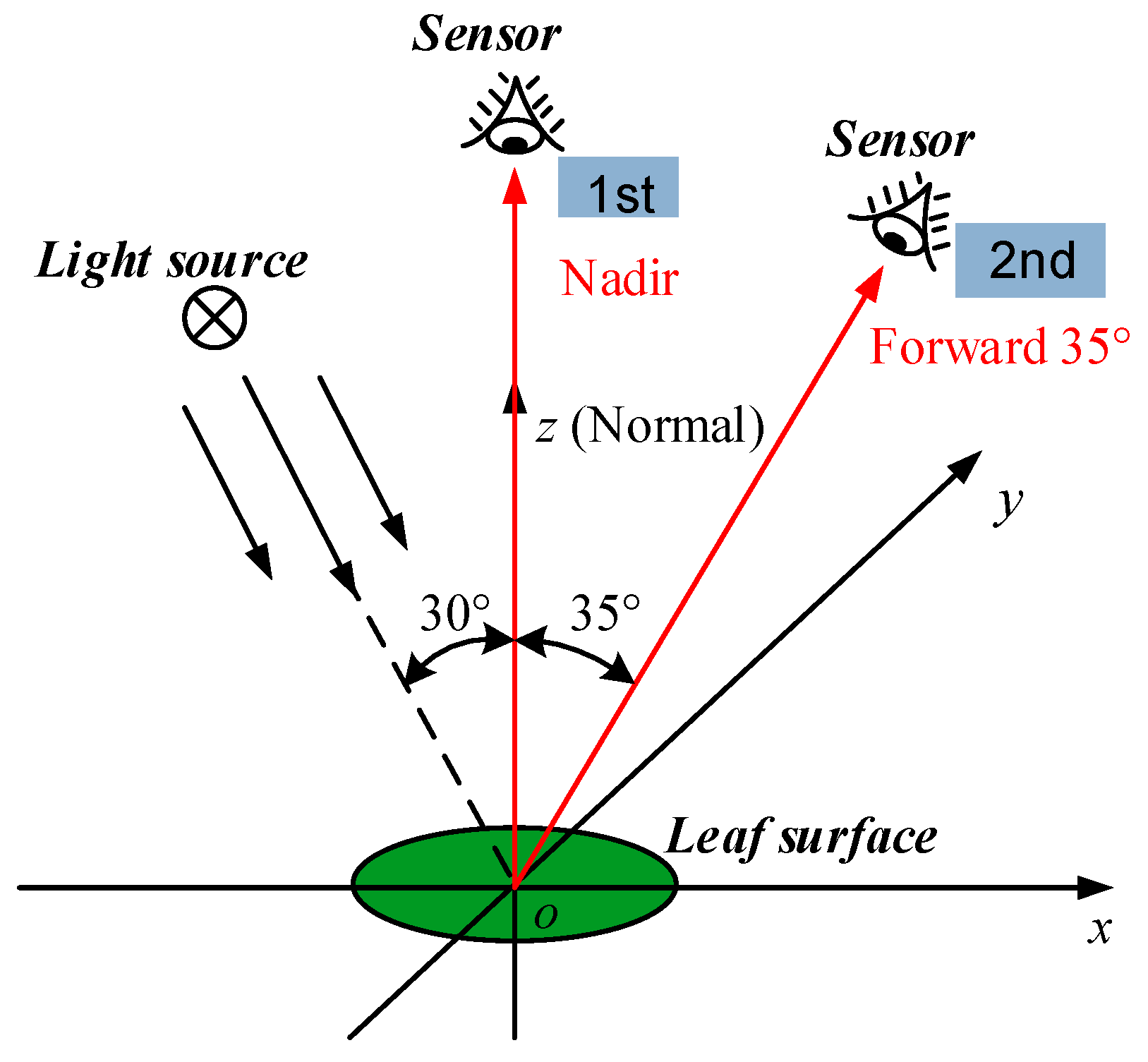
After sampling, the leaves were immediately transferred to the laboratory to measure reflectance with a spectroradiometer (Fieldspec 3 Hi-Res, ASD Inc., Boulder, CO, USA). This instrument has a spectral range of 350–2500 nm with a 3 nm and a 10 nm resolution in the visible and the near infrared regions, respectively. With a multi-angle platform [40], the zenith angle of the light source was fixed at 30°. Reflectance was measured in the conventional nadir and the forward 35° directions in the principle plane (formed by the illumination direction and leaf surface normal; the xoz-plane in Figure 1). The forward 35° direction rather than the mirror-like forward 30° direction was chosen, because specular reflectance reaches the maximum at a greater angle due to leaf roughness [13,41]. In the two directions, polarization data were also measured (details in [15]). The “mirror-like” term here was defined as being analogous to the direction of the Fresnel reflection. The measured reflectance was noisy at around 350 nm. Since the pigments mainly function in the visible region, only the data within 400–1000 nm were investigated in this study.
After spectral measurements, a disk was punched from each leaf with a borer. The disk was cut into fine pieces and soaked in a certain volume of 80% (v/v) acetone solutions in a cuvette. The cuvette was kept in the dark at room temperature for 48 h. The absorbance of the extract supernatant was measured at 663.2, 646.8, and 470 nm with a spectrophotometer (UV-2550, Shimadzu, Kyoto, Japan). The concentrations of chlorophyll a, chlorophyll b, total chlorophylls (chlorophyll a + b), and carotenoids were obtained as described previously [42]. The pigment content was a function of concentration, leaf area, and solution volume, and it was thus determined.
2.2. Data processing, Analysis, and Retrieval Methods
2.2.1. Continuous Wavelet Transformation
Wavelet analysis can be divided into continuous wavelet transform (CWT) and discrete wavelet transform (DWT). The coefficients after performing CWT on the spectral data can directly correspond to their original wavelengths, and they provide large amounts of information about the absorption features. However, the coefficients from DWT do not directly correspond to the wavelengths and they are difficult to interpret [43]. Considering our objectives, only CWT was performed.
However, one aspect of confusion in the application of wavelet transform is the arbitrary choice of wavelet function [44]. Torrence and Compo [44] suggested that the function should reflect the types of features in the original spectrum. We chose the second derivative of the Gaussian (DOG), knowns as Mexican Hat, as the function. Previous studies have suggested that the shapes of absorption features are Gaussian-relevant [45,46], and some authors have also used DOG in their studies (e.g., [36,47]). CWT was performed in MATLAB (Version R2016a, MathWorks) with the function cwt, on both the original reflectance and the first derivative. The decomposition was conducted at the dyadic scales: 21, 22, …, and 27, similar to in [25,35,43].
2.2.2. Multiple Linear Regression
Multiple linear regression (MLR) was used to build MLR-based retrieval models. To make the model as simple and as robust as possible, the most significant independent variables for explaining the response were selected, using the stepwise regression method. The criterion for keeping an independent variable in the model in stepwise multiple linear regression (SMLR), can be a sequence of F-tests, t-tests, the adjusted multiple coefficients of determination (adj. R2), etc. To distinguish the specular interference alleviation effect in different modes of spectral processing, the initial R2 without any spectral transformation should first be considered. Grossman et al. [48] called this the “baseline” coefficient of determination. Thus, the SMLR was conducted on the original reflectance first, and then on the first derivatives and wavelet coefficients. In these processes, the data derived at wavelengths (e.g., reflectance, etc.) were the independent variables, and the pigment content was the response. SMLR was performed in MATLAB (Version R2016a, MathWorks) with the function stepwise. The change in the adj. R2 value before and after adding an independent variable into the model was used as the criterion of keeping this variable.
Moreover, according to the authors of [49], when retrieving biochemical constituents with SMLR, the selected wavelengths and R2 values may vary considerably among different calibration and validation data subsets. Before determining the final model, the selection consistency of wavelengths should be examined. Therefore, 10 randomly extracted subsets each with 50 samples, and the entire dataset with all 68 samples, were, respectively, used for calibration. For two selections, if all of the distances between the two corresponding wavelengths were ≤10 nm, these two selections would be regarded as having good consistency, and vice versa. The consistency of a selection with the entire dataset was especially stressed. For example, the #7 selection in Table A4 is not very consistent with the “Entire”, because the wavelength pair of 555 and 580 nm has a distance of 25 nm > 10 nm. A distance of 10 nm is the minimum spectral resolution that the hyperspectral instrument should have, thus was used as the indicator here. To maximize the representativeness of the selections, the wavelengths selected from the entire dataset were used as the independent variables in the final models. All of the selections with SMLR in this study are provided in Figure S1.
2.2.3. Specular Removal and Specular Resistance Techniques
The above-mentioned approaches that especially take account of the specular reflectance or the specular effect in Section 1 are summarized in Table 1. They were tested in this study.
In Table 1, the column “Specular estimator” corresponds to the specular removal type, and it represents the term that estimates the specular reflectance or specular effect.
Rx in the column “Formula” for VIs represents the reflectance at the wavelength x nm. RNIR, Rred, and Rblue in SIPI means the wavelength is in the near-infrared, red, and blue regions, respectively. Here, we used 800, 675, and 445 nm, respectively. and in Rdiff-reSR and Rdiff-reND represent the diffuse reflectance at 800 and 710 nm, respectively. The diffuse reflectance was obtained at each wavelength from a simple model, using polarization measurements. In the MSC transformation:
where Smear is a measured reflectance spectrum, and Savg is the average reflectance spectrum from all samples. a and b are the two regression coefficients obtained by linear least squares. E is a unit vector, and e is the error vector after regression. The processed spectrum is:
Smear = aE + bSavg + e
mscSmear = (Smear – aE)/b
In the SNV transformation, the processed spectrum is:
where mean(Smear) and std(Smear) are, respectively, the mean and standard deviation of Smear. Clearly, the mathematical ideas behind MSC and SNV are similar, and the main difference lies in the selection of the reference (i.e., Savg and mean(Smear) here). Rk and Rh in the four-band RRDI have the local minima of the coefficient of variation across wavelengths, and then Rj and Ri are obtained from optimization (e.g., to make the R2 value of the VI vs. the pigment content the greatest).
snvSmear = [Smear – mean(Smear) × E] / std(Smear)
The RT and hybrid models are all based on the PROSPECT model [10]. PROSPECT was first developed in 1990, and it has been updated, with several versions being released. The latest version is PROSPECT-D [50], which adds the anthocyanin content parameter compared to the second-latest version, PROSPECT-5 [51]. We only used PROSPECT-D in the RT and the hybrid models. bspec in PROCOSINE is a complicated specular term, which is relevant to specular reflectance in BRF and directional hemispherical reflectance factor (DHRF), and it is retrieved in model inversion. In PROCWT, the specular reflectance in BRF and DHRF is regarded as being constant. Then, the constant term is reduced in CWT. In PROSPECT + R−445, the measured and simulated reflectance at 445 nm (R445) is used as a specular reflectance estimation, and it is subtracted from the measured and simulated reflectance, respectively. With the consequent “approximate” diffuse reflectance, the pigment content is retrieved with PROSPECT. Note that PROSPECT was originally developed for DHRF and the directional hemispherical transmittance factor (DHTF) simulation, where the incident zenith angle is 0°. Although PROCOSINE and PROCWT were applied to BRF and obtained good accuracies for their own datasets, their incident zenith angles were relatively small (≤20°). PROSPECT + Rdiff + R−445 is similar to PROSPECT + R−445, but Rdiff is used instead of the measured reflectance minus the measured R445. Rdiff here is the same as that in Rdiff-reSR and Rdiff-reND.
2.2.4. Statistics, Model Building, and Evaluation
Descriptive statistics such as the mean and range were made for the chlorophyll and carotenoid contents.
When retrieving the pigment content, as for MLR-based models, the entire dataset was randomly divided into two subsets in model building, one with 50 samples for calibration, and the other with 18 samples for validation. With the selected wavelengths from SMLR, MLR was conducted to calibrate the model on the calibration subset. With the calibrated model, the pigment content was predicted for the validation subset. This calibration-validation process was repeated 10 times. Each time, a root-mean-square error (RMSE) was obtained. The 10 RMSEs were averaged as the RMSE for this retrieval method. The relative error (RE) was also calculated:
where n is the number of samples, xi is the actual pigment content of the leaf numbered i, is the corresponding prediction for xi, and mean(content) is the average of the actual pigment contents of all leaves in the entire dataset. For each of the 10 calibration-validation processes, the estimated and actual contents were fitted with a linear model at a confidence level of 95%. The 10 obtained R2 values and 10 p-values were averaged. The mean values of R2, RMSE, and RE were the evaluation indicators for a retrieval method.
where is the mean of the actual contents of n samples. The RMSE was also calculated in wavelength selections with SMLR. Moreover, when conducting SMLR on the wavelet coefficients, the scale at which the selection produced the lowest RMSE and the highest adj. R2 value was determined as the optimal decomposition scale:
where t is the number of independent variables.
For VIs, the calibration and validation were similar, while a simple linear model between the VI and the pigment content was fitted.
For the RT and the hybrid models, the inversion consisted in optimization of (i.e., minimizing) the merit function:
where θ is the input parameter vector, λ is the wavelength at λmin–λmax (400–1000 nm), and Ssimu is the simulated reflectance. In PROSPECT + Rdiff + R-445, f(∙) and g(∙) indicate calculating Rdiff and subtracting the simulated R445, respectively. In other models, f(·) and g(·) are the same; they represent CWT in PROCWT, subtracting R445 in PROSPECT + R−445, and no processing in PROSPECT and PROCOSINE. The optimization of Equation (8) was performed in MATLAB (Version R2016a, MathWorks) using the function lsqcurvefit, with the trust-region-reflective algorithm. The bounds of each parameter in θ (Table 2) were derived, referring to the LOPEX’93 experiment [52], and they covered the chlorophyll and carotenoid content range in our dataset (Table 3). Anthocyanin and brown pigment contents were fixed at 0.
2.2.5. Summary of the Retrieval Methods
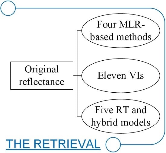
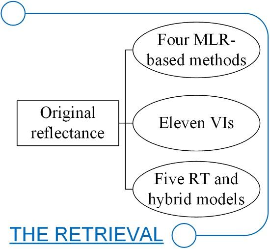
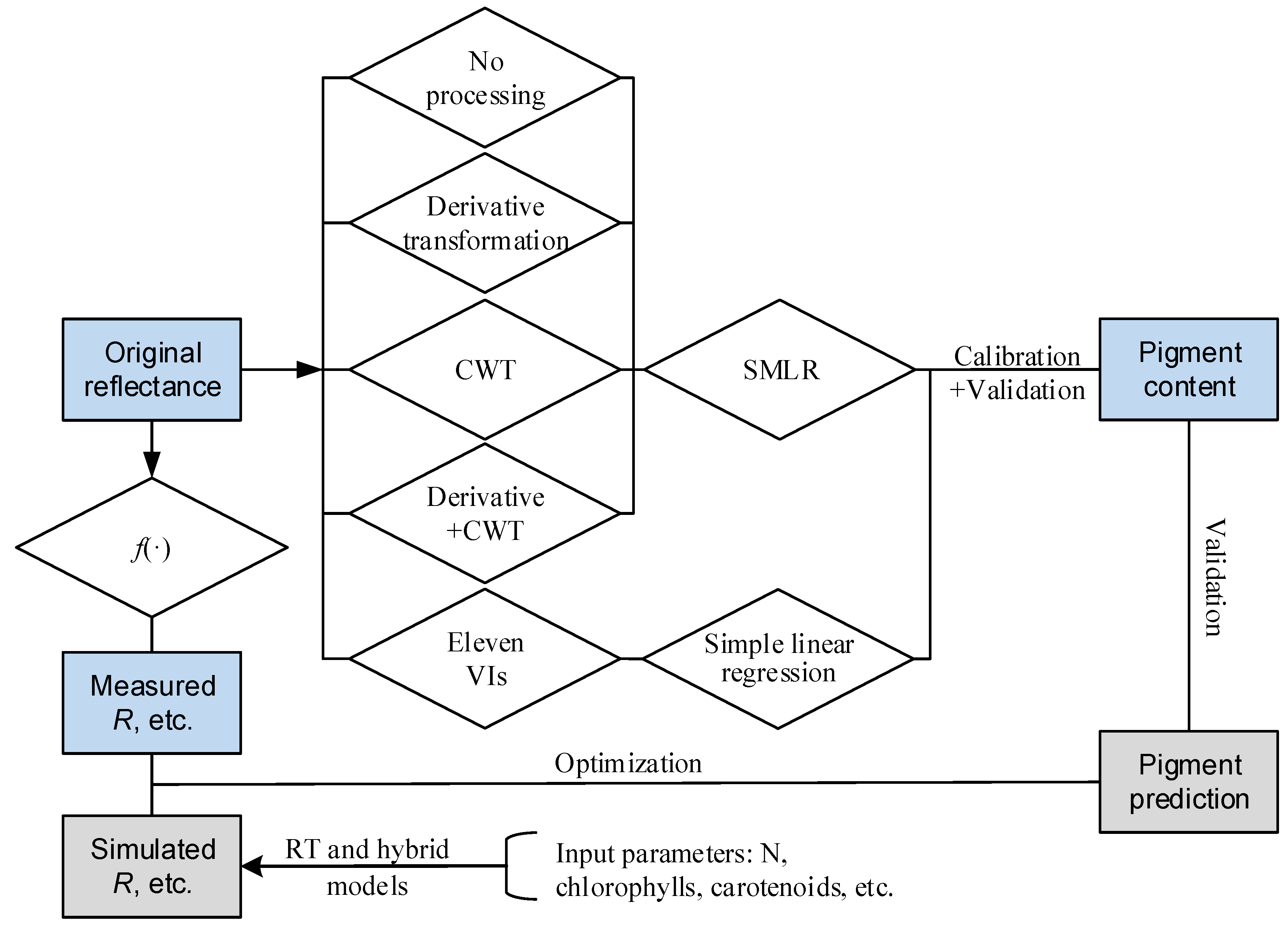
The main process of the retrieval techniques is illustrated in Figure 2. “SMLR” means using SMLR to search for the several optimal wavelengths. “No processing” means directly using the original reflectance for SMLR. “Derivative + CWT” means that the derivative transformation was performed on the original reflectance first, and then CWT was conducted on the obtained first derivatives.
3. Results
3.1. Statistics for Pigment Content
Table 3 shows the descriptive statistics for the chlorophyll and carotenoid contents. Mucuna had the largest mean, but the smallest range. This species is a type of evergreen vine. Pigments accumulate in the leaves with time, and hardly degrade in autumn and winter. On the contrary, the other two species are deciduous, and their pigments break down during these seasons, thus forming a relatively low mean and a wide range. The carotenoid and chlorophyll contents had a strong correlation, with a Pearson’s correlation coefficient of up to 0.96, which was significant at p < 0.01.
3.2. Leaf Reflectance Characteristics and Confusion Caused by the Effects of Specular Reflectance
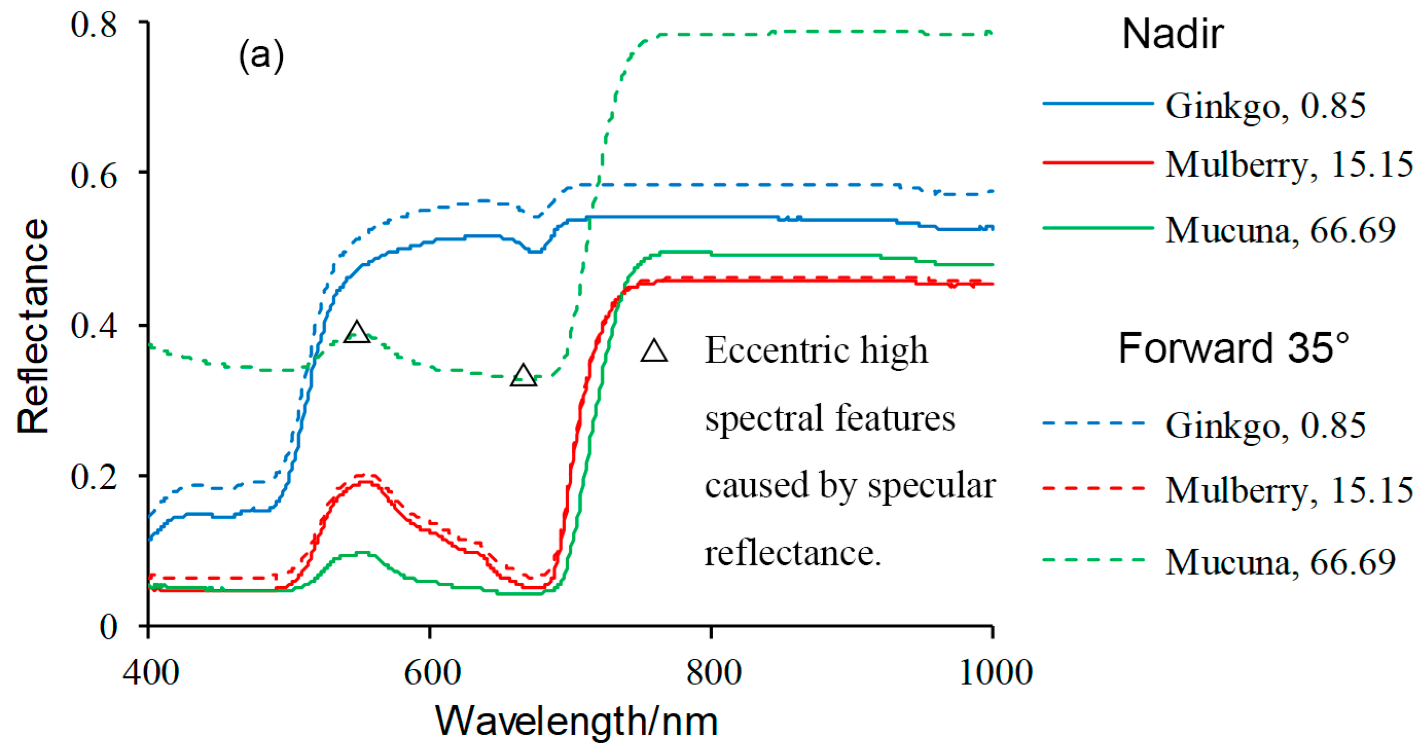
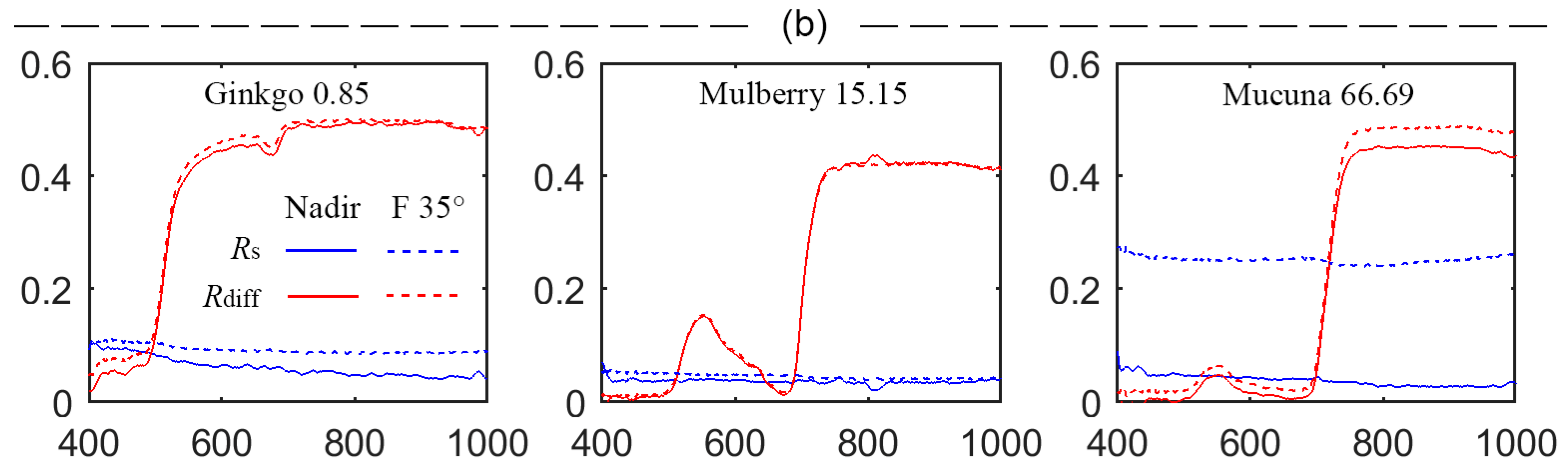
In the nadir direction, most samples showed the typical spectral characteristics of green leaves, as Figure 3a displays. The reflectance in the blue and red regions was low, due to the strong absorption by the pigments, while in the green region, a peak appeared because the absorption was relatively weak. In the near-infrared, there was a high plateau, owing to strong scattering by the leaf structure. Furthermore, with the increase in the pigment content, the reflectance in both major absorption regions decreased. The reflectance in the green region also dropped, but with a relatively low intensity. Based on these spectral feature changes with pigment content, a series of VIs were established to retrieve pigment content, such as the NDVI and the green ratio (RNIR/Rgreen) [53].
However, in the forward 35° direction, the situation was different. Leaf reflectance was always larger in this direction than in the nadir, especially for the mucuna leaves (Figure 3a and Figure 4). Since leaf diffuse reflectance was isotropic in directions [13,14], the higher reflectance in this direction was due to a greater amount of specular reflectance (Figure 3b and Table 4). The specular reflectance in Figure 3b and Table 4 was obtained with a simple model, through polarization measurements [15]. Note that the reflectance of the mucuna leaf at 800–1000 nm in Figure 3a reached almost 0.80, and in the green and red regions, it was still higher than that of the mulberry leaf. However, the chlorophyll content of the former was much higher than that of the latter (66.69 vs. 15.15 μg/cm2). This was a contradiction to the nadir trend, where more pigments would result in a lower reflectance in the major absorption regions. Therefore, this unusual spectral feature change would cause confusion in pigment content retrieval, and usually induces a decrease in retrieval accuracy (e.g., using previous green ratio [15]).
3.3. Pigment Content Retrieval
3.3.1. VIs, RT, and Hybrid Models
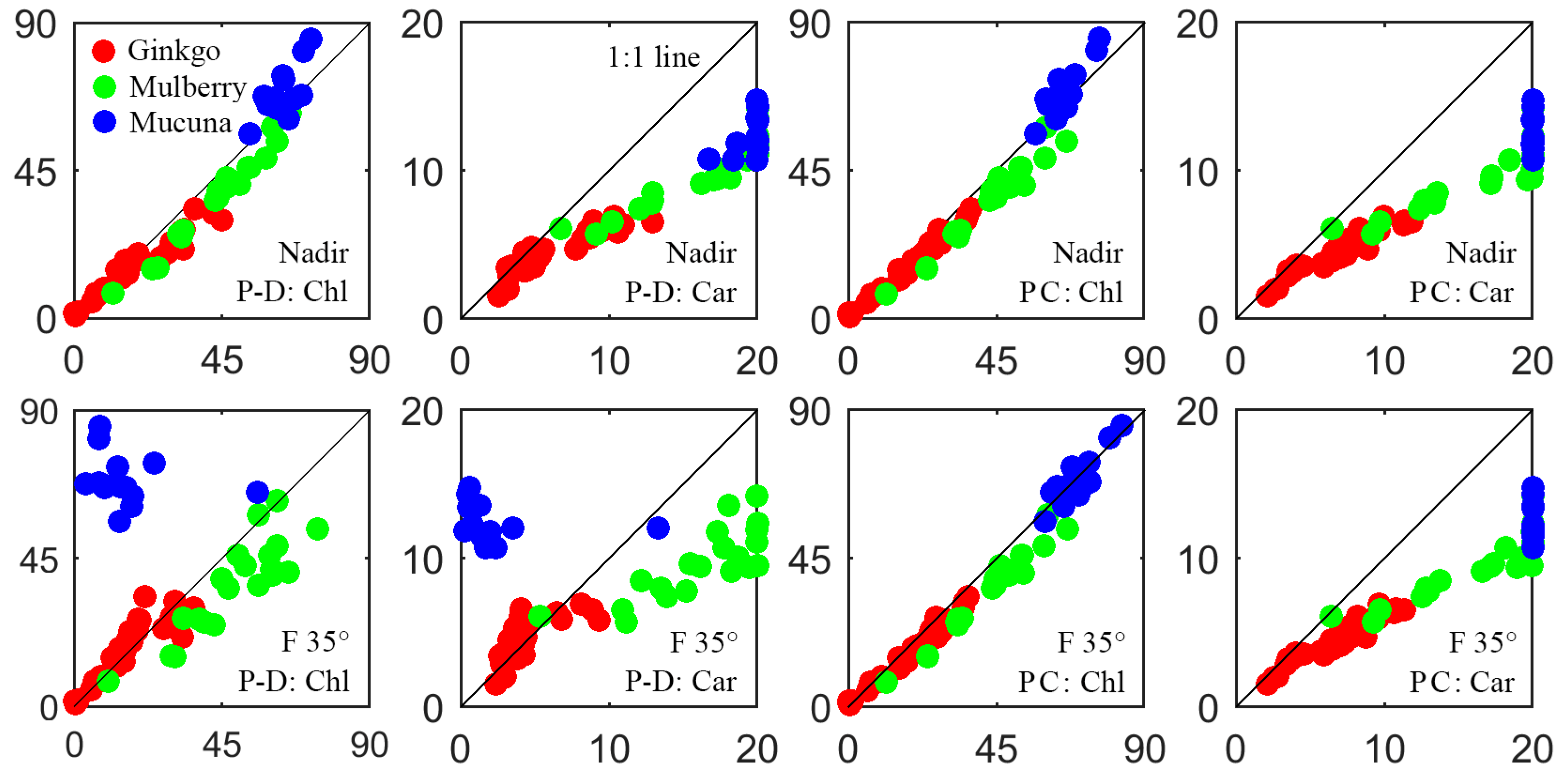
Table 5 shows the validation results for the RT and hybrid models. For chlorophylls, with higher specular reflectance in the forward 35° direction, the retrieval accuracy with PROSPECT-D decreased considerably compared to that in the nadir direction (RE: 80.40% vs. 19.57%). All of the other approaches reduced the specular interference in the forward 35° direction, and produced comparable results (except PROCWT) between the two viewing directions. For example, the RE of PROCOSINE was 15.05% and 15.62% in the forward 35° and nadir directions, respectively. However, these models could not retrieve the carotenoid content, due to the large errors (all REs > 58%). Overall, the retrieval appeared to be ill-posed, and these models were not appropriate for our measurement geometry with a 30° incident zenith angle. Although PROCWT and PROCOSINE were applicable for BRF data in some studies, the incident zenith angle was relatively small (≤20°). Under these circumstances, the specular component took up only a small proportion of the total DHRF at 400–1000 nm (e.g., <0.1 for corn and soybean leaves [54]), and the diffuse reflectance in DHRF and BRF was considered to be equal [18,25].
Table 6 shows the validation with the 11 VIs. Unlike the RT and hybrid models, all of these VIs were simultaneously applicable for chlorophylls and carotenoids. R-reSR and R-reND were not specific for specular disturbance alleviation. Rdiff-reSR and Rdiff-reND were their counterparts, respectively, where specular reflectance was removed. From RMSEs and REs of these four VIs, it was clear that specular reflectance interfered with the retrieval, and that specular removal reduced the interference and improved the retrieval. For example, without removal, the RE of R-reSR for chlorophylls increased from 17.45% to 53.10% from the nadir to the forward 35° direction. In the forward 35° direction, after removal, this value decreased to 19.00%, and it was comparable to 13.77% in the nadir direction. With these four VIs as a reference, it was clear that each VI (except SIPI) obtained comparable accuracy in the two directions, and they effectively alleviated the specular disturbance in the forward 35° direction. SIPI had the worst results for both chlorophylls and carotenoids. This VI was originally designed for the relative carotenoid/chlorophyll a content, so it may be not suitable for absolute content retrieval. The four-band RRDI had the highest accuracy for both chlorophylls and carotenoids. Compared to the four-band RRDI (where k = h) mSR705, one more wavelength may increase the retrieval power of the VI.
3.3.2. MLR Using the Original Reflectance and the First Derivatives
In our preliminary experiment on original reflectance, for the chlorophyll content, the adj. R2 values increased with the number of independent variables, and remained constant when the number exceeded 3. To avoid overfitting and overestimation, the number of selected wavelengths was ≤3. For carotenoids, with three selected wavelengths, two of them were around 710 nm, with a distance of almost always less than 3 nm. To avoid such a correlation, no more than two wavelengths were selected. To allow a comparison, the maximum number of selected wavelengths was fixed, with three for chlorophylls and two for carotenoids in all of the MLR-based models.
Table 7 and Table 8 show the respective validation results using MLR for the original reflectance and the first derivatives. The accuracy was lower in the forward 35° than in the nadir direction for both chlorophylls and carotenoids, owing to the interference created by a larger amount of specular reflectance in the former direction (Table 7). Chlorophylls were more intensely disturbed than carotenoids (RE: 9.54–12.89% for chlorophylls vs. 14.44–15.09% for carotenoids). This different effect may be partly due to the content range, where chlorophylls were more abundant than carotenoids in the leaves (Table 3). Moreover, for chlorophylls, the retrieval in Table 7 was better than Rdiff-reSR (Table 5), and, for carotenoids, it approached mSR705. This was manifested in the effective specular resistance capabilities of the MLR models.
The derivative transformation can remove low-frequency background signals in the spectra [55]. Since leaf specular reflectance in a direction remained stable across wavelengths (Figure 3b) [13], it can be regarded as a constant (additive) term. Thus, the derivative transformation effectively reduced specular reflectance. Moreover, this transformation enhanced the spectral features (Figure 7). Compared to Table 7, Table 8 always has lower RMSE and RE values. This revealed that the derivative transformation plus MLR not only alleviated the specular interference but also further improved the retrieval. The improvement was more remarkable in the forward 35° direction than in the nadir direction for both pigments. For example, the RE for carotenoids decreased by 3.02% in the forward 35° direction, while it decreased by 1.84% in the nadir direction.
3.3.3. CWT plus MLR
Table 9 presents validation results with the CWT plus MLR method, at the optimal decomposition scales. Compared to Table 7, with the original reflectance input, the CWT plus MLR method further reduced the RMSE and RE for both chlorophylls and carotenoids in either direction. With the specular reflectance as a constant term, CWT reduced it, due to the linear additive property in wavelet analysis [25,47]. At the optimal decomposition scale, CWT enhanced the spectral features (Figure 7). Thus, the CWT plus MLR method not only effectively alleviated the specular disturbance but also further improved the retrieval. Moreover, after performing CWT on the reflectance or the derivatives, the retrieval with the wavelet coefficients nearly achieved the best results for both pigments among all of the methods in either direction. Of these CWT plus MLR models, the accuracy for either direction was higher for chlorophylls than for carotenoids (e.g., the nadir RE: 8.15% for chlorophylls vs. 11.55% for carotenoids), while for either pigment, the retrieval in the forward 35° direction was slightly better than that in the nadir direction (e.g., RE for carotenoids: 11.29% in the forward 35° direction vs. 11.55% in the nadir direction).
4. Discussion
4.1. The Effects of the Specular Disturbance Alleviation Methods
From the above results, the RT and hybrid models appeared to be ill-posed, and they obtained very high errors for carotenoids in the retrieval. Figure 5 displays the results with PROSPECT-D and PROCOSINE. Evidently, these models were not applicable under the geometry with an incident zenith angle = 30° for BRF. At such a high angle (>20°), BRF was markedly anisotropic in directions, and the anisotropy increased with the incident zenith angle. For example, the maxima of bidirectional reflectance distribution function (BRDF; BRF = BRDF × π) for the European beech (Fagus sylvatica L.) leaf ranged from 0.03 sr−1 at 5° to 0.45 sr−1 at 65° [56]. In our dataset, the mucuna leaves had large reflectance differences between the two viewing directions (Figure 3a and Figure 4), so the retrieval was poor (Figure 5). However, the bidirectional transmittance distribution function (BTDF) for leaves was much more isotropic than BRDF [12,54,56]. If leaf transmittance can be included in the models, or if new models are developed for transmittance, retrievals at high incident zenith angles (>20°) may be improved. This needs to be further studied.
In addition, in PROSPECT inversion, two other strategies were also examined: (1) only the visible range was used, and other parameters that were insensitive to the visible were fixed [25]; and (2) the whole spectrum was used and all input parameters varied [43]. For Strategy (1), the reflectance within 400–800 nm was used, and Cw was fixed at 0. For Strategy (2), the reflectance within 400–2200 nm was used (data at < 400 nm and > 2200 nm were discarded, due to high noise). For Strategies (1) and (2), anthocyanin and brown pigment contents were fixed at 0. The model was inverted according to the method in Section 2.2.4. The results were also ill-posed and they were generally not much different from those in Table 5.
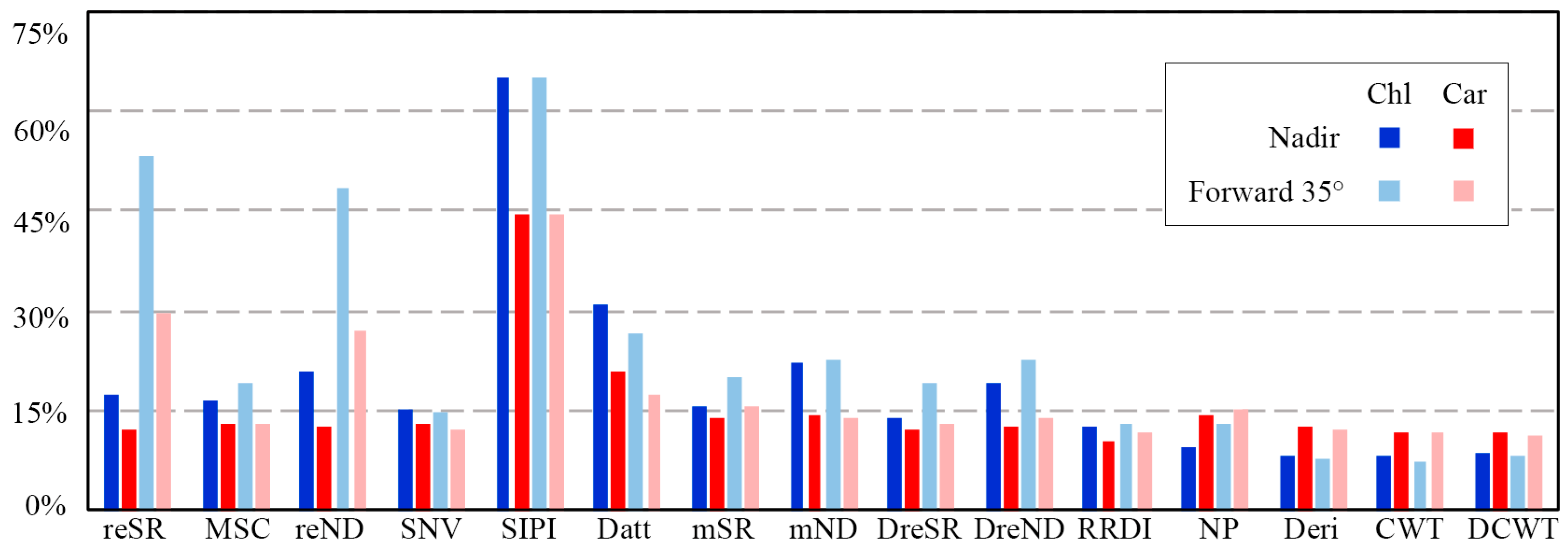
For the empirical techniques, the REs in Table 6, Table 7, Table 8 and Table 9 are illustrated in Figure 6. Again, it is clear that, compared to the VIs, the four MLR-based methods not only effectively alleviated specular interference, but also further improved the retrieval for both chlorophylls and carotenoids in either direction, especially for chlorophylls in the forward 35° direction. There may be two reasons for this: First, the linear combination of data at the specified wavelengths eliminated the low-frequency information. Table 10 demonstrates this situation. As specular reflectance can be regarded as a constant term, it was reduced by the combination of the positive and negative terms of the MLR models. Second, the coefficients, selected wavelengths, and constant terms were optimized for different data. Thus, the optimization not only effectively reduced the specular effect but also improved the retrieval. In addition, both the derivative transformation and CWT suppressed specular interference and enhanced the absorption features (Figure 7). Coupling either or both with MLR further improved the retrieval. However, it should be pointed out that the retrieval was surprisingly accurate (R2 ≥ 0.98 in Table 7, Table 8 and Table 9), and the improvement among these methods was generally marginal (e.g., compare Table 8 and Table 9). The reason for this may be that our dataset was quite limited (68 samples from three species). Thus, more samples and species should be added to the dataset. Under such circumstances, with a wider variation of leaf traits, these MLR-based methods need to be further examined for their applicableness and robustness.
For each of the four MLR-based methods, in either direction, the retrieval accuracy for carotenoids was always lower than that for chlorophylls. This may be due to the lower content of carotenoids vs. chlorophylls and the overlapping absorption regions of the two pigments. This would lead to interference from chlorophylls in carotenoid content retrieval, making the retrieval more challenging [57].
4.2. Pigment Content Retrieval with CWT
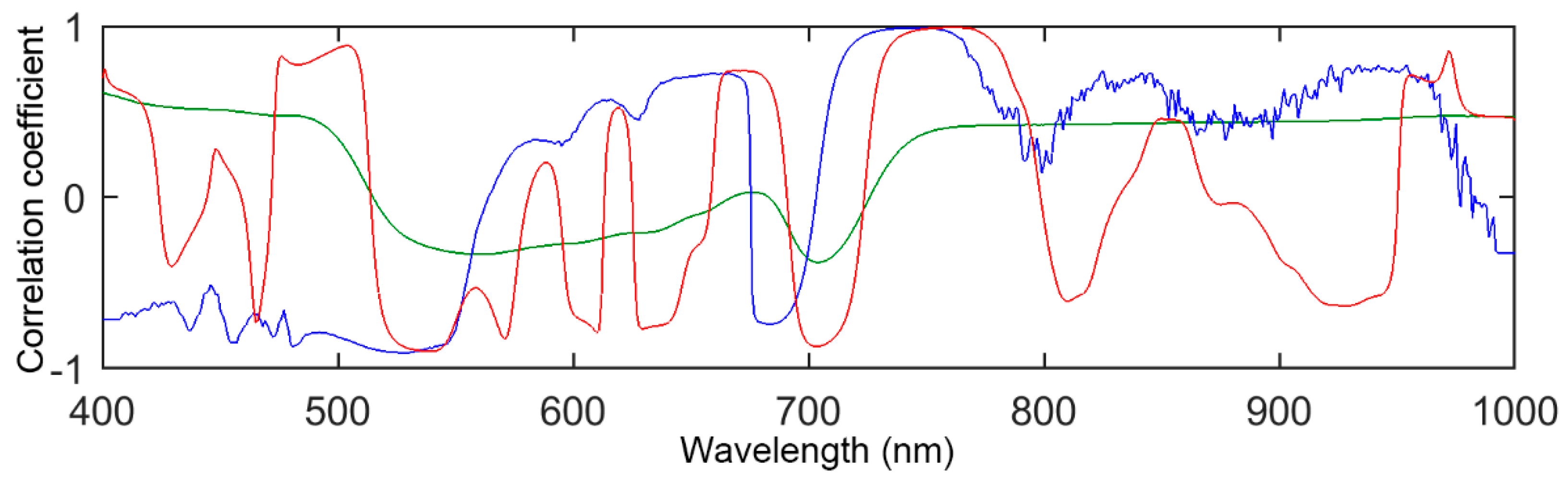
Figure 7 displays the correlation coefficients between the data derived at each wavelength and the chlorophyll content in the forward 35° direction. After the derivative transformation or CWT, the spectral features were significantly enhanced. For example, the absolute r value increased from 0.32 and 0.35 at 550 and 710 nm, respectively, to >0.85. In addition, intense micro-fluctuations on the blue line are noted, at approximately 400–450 nm and 770–1000 nm, which may be induced by high-frequency noise in the first derivative spectra. Although the derivative transformation reduced low-frequency signals (e.g., specular reflectance), it simultaneously increased high-frequency noise in the data [55]. This noise was then amplified when calculating correlation coefficients. However, CWT did not generate such noise, as indicated by the smooth red line in these regions. For carotenoids and the nadir direction, there was a similar situation (figure not shown).
On the optimal wavelet decomposition scale for retrieval, the scale for chlorophylls was 8 with original reflectance input in both directions, which was different from those in [25,35,43]. In [25], it was 16, 32, and 16 for wheat, rice, and wheat + rice, respectively, using PROCWT (PROSPECT-D used). In [43], it was 64 and 32, respectively, for PROSPECT- and LIBERTY-simulated [58] reflectance, both with the first derivative input. In [35], it was 64 for the PROSPECT-simulated reflectance, and the accuracies with reflectance and the first derivative input were equivalent. In addition, the authors of [35,43] used only simulated data with a wide variation of leaf traits, while we used measured data that contained only 68 samples from three species with a relatively narrow range of such variation. For carotenoids, in [25], the scale was 32, 64, and 32 for wheat, rice, and wheat + rice, respectively. In our study, the scale was 4, with the original reflectance input in the nadir direction, and 64 with the first derivative input in the forward 35° direction.
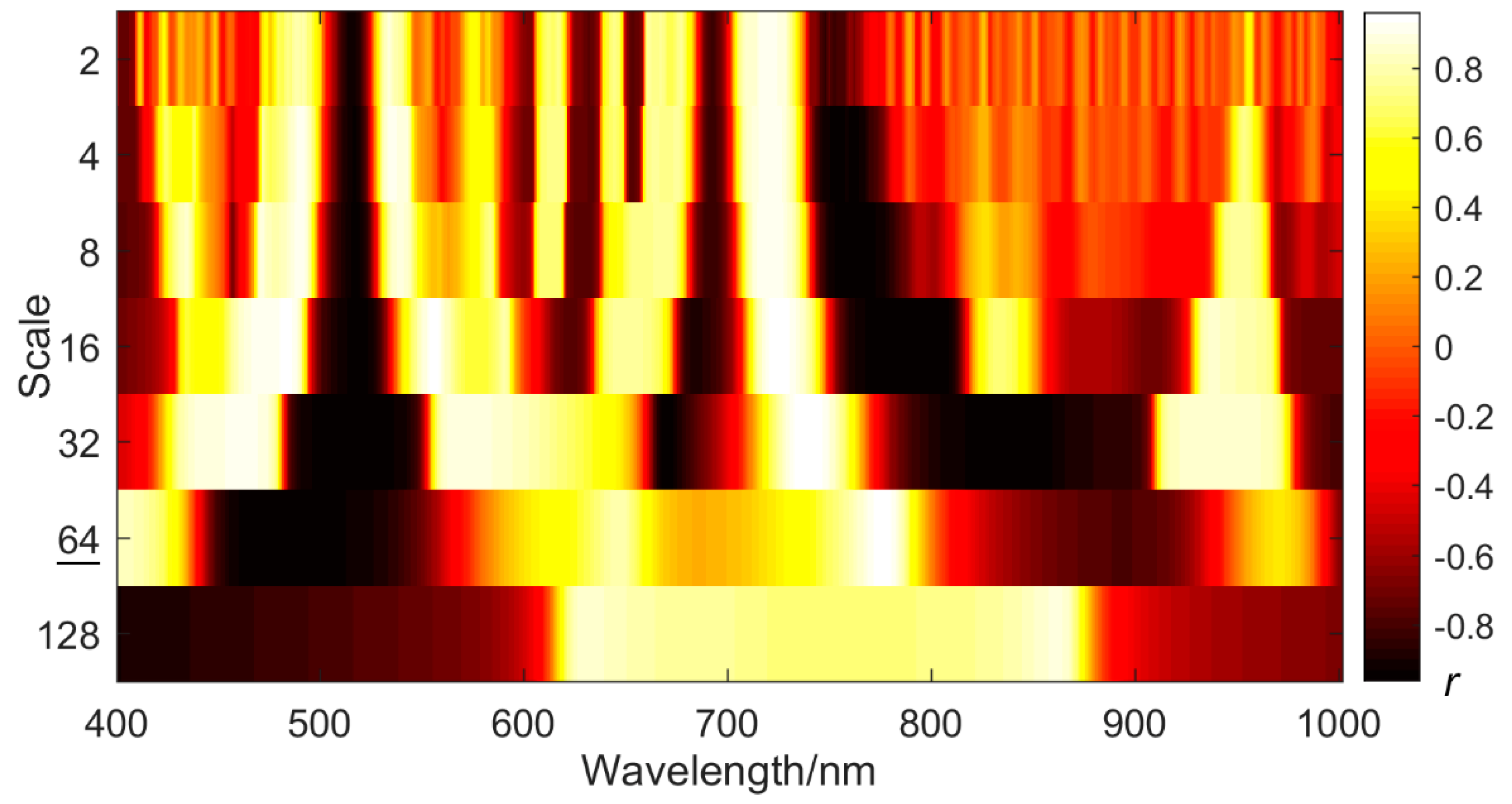
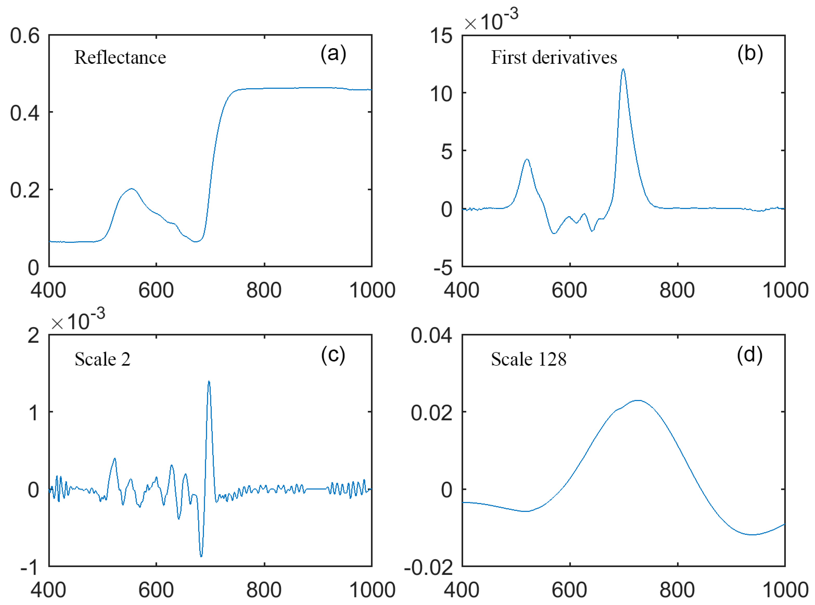
In all of these studies, the optimal scales for pigment content retrieval were generally located near the intermediate position among the decomposition scales (e.g., 32 in 2, 4, 8, …, 128). At a lower decomposition scale, the wavelet coefficients corresponded to noise and fine absorption features, while, at a higher scale, they corresponded to the broad features and leaf structures that determined the overall shape of the reflectance spectra [43]. Thus, the best scale for retrieval may appropriately respond simultaneously to these factors, resulting in a balance among them. Figure 8 and Figure 9 demonstrate this situation. Notice the intense narrow colored stripes and micro-fluctuations at a scale of 2 in Figure 8 and Figure 9c, respectively. When the scale was larger (e.g., 128), these stripes gradually merged into wider colored blocks (Figure 8), and the micro-fluctuations disappeared, forming a smooth generalized curve (Figure 9d). The optimal scale (e.g., 64 in Figure 8) achieved a compromise for this change.
4.3. Selected Wavelengths and Selection Consistency with SMLR
All of the selections for searching for the best wavelengths for chlorophyll and carotenoid content retrieval with SMLR are provided in Figure S1. The selections with the best scales are shown in Table 9 (underlined), and the selections based on the original reflectance in the two directions are presented in the Appendix A.
For the best scales in Table 9 (Table A2, Table A3, Table A4 and Table A5), the percentages of wavelength consistency in the selections were rather low (<0.5), but all of the selections for a pigment in a particular direction had almost the same adj. R2 values. For the selections based on reflectance (Table A1), the consistency was high (percentage ≥ 0.7), and the adj. R2 values were not much different (the R2 value difference was generally ≤ 0.02), for a pigment in either direction. It seems that the percentage of selection consistency decreased for the MLR models with the processed data, compared to those with the original data. The reason for this may be that the CWT corresponded to and enhanced the spectral features, resulting in wavelet coefficients that were more variable than the reflectance. Thus, greater differences should be contained among the extracted subsets of the processed data than those of the original reflectance, for a given calibration-validation process. Besides, the selections with reflectance were very different from those in [49], whose R2 values (less than ours) and wavelength selection consistencies varied greatly, depending on the calibration and validation subsets. This distinction may be caused by two reasons. First, the dataset in [49] contained 50 species, covering a much wider variation of leaf traits than ours, with only three species. Second, in the visible region, the spectral signals were dominated by pigments, and these signals were very strong. However, the signals of lignin, cellulose, starch, etc., were located in the near-infrared region. These signals were relatively weak, and they were often overlapped by water in fresh leaves, and they were susceptible to many other factors, such as noise. All of these reasons may prevent calibrations from attaining good wavelength selection consistency and high retrieval accuracy.
For the wavelengths selected for reflectance, for chlorophylls and carotenoids in both directions, there was always a wavelength that was located in the red edge region (around 710 nm, Table A1). This revealed the significance of this range for both the chlorophyll and carotenoid content retrievals, even when a large amount of specular reflectance existed. For chlorophylls, another wavelength was situated at around 780 nm. These two wavelengths can be used to build VIs, such as the RNIR/Rred edge region [11], to retrieve the pigment contents. In addition, with the reflectance at 450 and 675 nm as independent variables, the MLR models were examined using the same process in Section 2.2.4 to retrieve the chlorophyll content. The RMSEs were 18.08 and 16.04 μg/cm2 in the nadir and forward 35° directions, respectively. Thus, with only the main absorption features, chlorophyll content cannot be accurately retrieved.
4.4. About the Application of Our Methods at a Canopy Scale
At a canopy scale, specular reflectance may cause a confusion in the biochemical content estimation, such as photosynthetic activity [16], vegetation amount [59], and chlorophyll content [24]. However, the specular reflection at a canopy scale is quite complicated. All the factors, such as the phenology, plant physiological phases, and stress, which can affect canopy structure, may influence canopy specular reflection. This situation may complicate the relationship between specular reflectance and biochemical content as well. This issue has not been fully studied so far. Thus, the methods proposed in this paper at a leaf scale should be further investigated when being applied at a canopy scale.
5. Conclusions
In this study, several VIs, RT, and hybrid models that specifically take account of the specular reflectance or specular effect, and wavelet analysis, were investigated to retrieve the pigment contents in the nadir and oblique viewing directions at a leaf scale.
Although the RT and hybrid models confirmed their applicableness with high accuracy at a low incident zenith angle (≤20°) in some studies, their retrievals appeared to be ill-posed at a higher angle of 30°.
For the empirical methods, all eight of the VIs, namely MSC + R-reSR, SNV + R-reND, Datt_710, mSR705, mND705, Rdiff-reSR, Rdiff-reND, and four-band RRDI, obtained comparable accuracies between the two directions, and they could effectively alleviate the specular disturbance in the forward 35° direction. Of these VIs, the four-band RRDI performed the best for both chlorophylls and carotenoids.
The MLR, derivative transformation, and CWT could alleviate the specular interference as well. Moreover, the MLR-based methods generally obtained higher retrieval accuracies than the VIs. For these MLR-based methods, the retrieval for chlorophylls was always better than for carotenoids. Among all of the methods investigated, CWT plus MLR was outstanding, and it generally achieved the best retrieval for both pigments. The results are 2.68 and 0.88 μg/cm2 for chlorophylls and carotenoids, respectively, in the nadir direction, and 2.42 and 0.86 μg/cm2 in the forward 35° direction. Of the decomposition scales with CWT, the low scale corresponded to the noise and fine absorption features, while the high scale characterized the broad absorption features and leaf structure properties that defined the overall reflectance shape. The optimal scale for retrieval probably lays near the intermediate position (e.g., 32 in 2, 4, 8, …, 128), appropriately resulting in a balance among the effects of these factors.
Although excellent results were obtained with the MLR-based methods, they were based on a limited dataset, with 68 samples from three species, and the improvements among these methods were slight. More samples and leaf species should be added to the dataset, to enlarge the variation of leaf traits. The approaches proposed must be verified under a context of wider variation to investigate their performance and robustness. More effort should be made for carotenoid content retrieval, due to its difficulty, and also due to the critical role of this pigment in plant physiology and ecology. In addition, the relationship between specular reflectance and biochemical content at the canopy scale should be further studied. The application of our methods at this scale also needs more investigation.
Supplementary Materials
The following are available online at https://0-www-mdpi-com.brum.beds.ac.uk/2072-4292/11/8/983/s1, Table S1: SMLR_Selection_Data.xlsx.
Author Contributions
The research concept was initially proposed by J.H., in discussion with Y.L. Y.L. designed and performed the experiment. Y.L. wrote the initial manuscript. J.H. significantly reviewed and edited the manuscript.
Funding
This research was funded by the National Natural Science Foundation of China, grant number 41471277.
Acknowledgments
The authors appreciate Shikai Fan’s (Institute of Agricultural Chemistry, Zhejiang University) sincere help in the chemistry experiments, and Yao Zhang’s (Institute of Applied Remote Sensing and Information Technology, Zhejiang University) valuable assistance in the chemistry experiments and spectral measurements. The authors are also grateful to the anonymous reviewers for their detailed and constructive comments that vastly improved the manuscript.
Conflicts of Interest
The authors declare no conflict of interest.
Appendix A

Table A1.
Selections with SMLR on the original reflectance. “Entire” means all that 68 leaves in the dataset were used. In total, 41 datasets (40 subsets + 1 entire set) were used. Adj. R2 indicates adjusted R2. The selections whose wavelengths are far (>10 nm) from the corresponding “Entire” are marked in bold (indicating poor consistency). These abbreviations and symbols have the same meanings as in Table A2, Table A3, Table A4 and Table A5. All adj. R2 values have a p-value < 0.01.
| Nadir | Wavelength/nm | Adj. R2 | RMSE/ μg·cm−2 | Forward 35° | Wavelength/nm | Adj. R2 | RMSE/ μg·cm−2 | |||||
|---|---|---|---|---|---|---|---|---|---|---|---|---|
| Chlorophylls | #1 | 711 | 725 | 784 | 0.98 | 2.93 | #1 | 400 | 713 | 780 | 0.96 | 4.58 |
| #2 | 711 | 728 | 772 | 0.98 | 3.25 | #2 | 400 | 713 | 775 | 0.96 | 4.55 | |
| #3 | 710 | 724 | 784 | 0.98 | 2.69 | #3 | 400 | 712 | 773 | 0.96 | 4.64 | |
| #4 | 712 | 727 | 772 | 0.98 | 3.32 | #4 | 400 | 713 | 773 | 0.96 | 4.64 | |
| #5 | 711 | 725 | 771 | 0.98 | 2.95 | #5 | 400 | 712 | 779 | 0.96 | 4.50 | |
| #6 | 710 | 725 | 772 | 0.99 | 2.77 | #6 | 400 | 714 | 788 | 0.96 | 4.58 | |
| #7 | 709 | 725 | 770 | 0.98 | 3.16 | #7 | 400 | 711 | 770 | 0.96 | 4.43 | |
| #8 | 711 | 725 | 772 | 0.98 | 2.79 | #8 | 400 | 713 | 975 | 0.97 | 3.63 | |
| #9 | 711 | 731 | 772 | 0.98 | 2.88 | #9 | 400 | 713 | 788 | 0.96 | 4.60 | |
| #10 | 710 | 728 | 771 | 0.98 | 3.29 | #10 | 443 | 700 | 705 | 0.94 | 5.60 | |
| Entire | 710 | 725 | 772 | 0.98 | 3.14 | Entire | 400 | 713 | 780 | 0.96 | 4.40 | |
| Carotenoids | #1 | 714 | 769 | 0.92 | 1.03 | #1 | 437 | 705 | 0.91 | 1.14 | ||
| #2 | 405 | 714 | 0.93 | 1.00 | #2 | 437 | 705 | 0.91 | 1.14 | |||
| #3 | 714 | 769 | 0.92 | 1.06 | #3 | 439 | 706 | 0.92 | 1.09 | |||
| #4 | 711 | 771 | 0.92 | 0.97 | #4 | 439 | 705 | 0.89 | 1.24 | |||
| #5 | 714 | 769 | 0.92 | 1.06 | #5 | 400 | 716 | 0.92 | 1.02 | |||
| #6 | 714 | 770 | 0.92 | 1.09 | #6 | 434 | 706 | 0.91 | 1.08 | |||
| #7 | 712 | 771 | 0.91 | 1.08 | #7 | 439 | 706 | 0.90 | 1.18 | |||
| #8 | 714 | 784 | 0.92 | 1.08 | #8 | 438 | 706 | 0.91 | 1.19 | |||
| #9 | 714 | 784 | 0.93 | 1.06 | #9 | 439 | 705 | 0.90 | 1.20 | |||
| #10 | 715 | 768 | 0.93 | 1.01 | #10 | 504 | 705 | 0.92 | 1.09 | |||
| Entire | 714 | 769 | 0.92 | 1.02 | Entire | 439 | 705 | 0.91 | 1.15 | |||
Table A2.
Selections on the wavelet coefficients (original reflectance input, scale 8) where the retrieval for chlorophylls is the best in the nadir direction (Table 9). All adj. R2 values have a p-value < 0.01.
Table A2.
Selections on the wavelet coefficients (original reflectance input, scale 8) where the retrieval for chlorophylls is the best in the nadir direction (Table 9). All adj. R2 values have a p-value < 0.01.
| Scale 8 | Wavelength | Adj. R2 | RMSE | ||
|---|---|---|---|---|---|
| #1 | 625 | 764 | 897 | 0.99 | 2.37 |
| #2 | 569 | 706 | 763 | 0.99 | 2.42 |
| #3 | 764 | 877 | 975 | 0.99 | 2.19 |
| #4 | 551 | 765 | 818 | 0.99 | 2.39 |
| #5 | 763 | 877 | 975 | 0.99 | 2.41 |
| #6 | 568 | 708 | 763 | 0.99 | 2.21 |
| #7 | 568 | 708 | 764 | 0.99 | 2.21 |
| #8 | 569 | 763 | 874 | 0.99 | 2.64 |
| #9 | 565 | 686 | 764 | 0.99 | 2.34 |
| #10 | 568 | 765 | 875 | 0.99 | 2.19 |
| Entire | 568 | 708 | 764 | 0.99 | 2.39 |
Table A3.
Selections on the wavelet coefficients (original reflectance input, scale 4) where the retrieval for carotenoids is the best in the nadir direction (Table 9). All adj. R2 values have a p-value < 0.01.
Table A3.
Selections on the wavelet coefficients (original reflectance input, scale 4) where the retrieval for carotenoids is the best in the nadir direction (Table 9). All adj. R2 values have a p-value < 0.01.
| Scale 4 | Wavelength | Adj. R2 | RMSE | |
|---|---|---|---|---|
| #1 | 527 | 751 | 0.95 | 0.85 |
| #2 | 528 | 753 | 0.94 | 0.87 |
| #3 | 750 | 992 | 0.95 | 0.84 |
| #4 | 751 | 990 | 0.95 | 0.83 |
| #5 | 505 | 766 | 0.94 | 0.91 |
| #6 | 528 | 752 | 0.94 | 0.88 |
| #7 | 529 | 752 | 0.94 | 0.86 |
| #8 | 529 | 750 | 0.95 | 0.87 |
| #9 | 529 | 752 | 0.94 | 0.96 |
| #10 | 751 | 993 | 0.96 | 0.77 |
| Entire | 750 | 1000 | 0.95 | 0.82 |
Table A4.
Selections on the wavelet coefficients (original reflectance input, scale 8) where the retrieval for chlorophylls is the best in the forward 35° direction (Table 9). All adj. R2 values have a p-value < 0.01.
Table A4.
Selections on the wavelet coefficients (original reflectance input, scale 8) where the retrieval for chlorophylls is the best in the forward 35° direction (Table 9). All adj. R2 values have a p-value < 0.01.
| Scale 8 | Wavelength | Adj. R2 | RMSE | ||
|---|---|---|---|---|---|
| #1 | 469 | 578 | 762 | 0.99 | 2.34 |
| #2 | 579 | 715 | 763 | 0.99 | 2.30 |
| #3 | 579 | 717 | 762 | 0.99 | 2.30 |
| #4 | 582 | 761 | 839 | 0.99 | 2.01 |
| #5 | 579 | 762 | 861 | 0.99 | 2.44 |
| #6 | 582 | 761 | 863 | 0.99 | 2.28 |
| #7 | 555 | 761 | 862 | 0.99 | 2.29 |
| #8 | 625 | 762 | 863 | 0.99 | 2.35 |
| #9 | 581 | 760 | 861 | 0.99 | 2.46 |
| #10 | 581 | 760 | 862 | 0.99 | 2.19 |
| Entire | 580 | 761 | 862 | 0.99 | 2.30 |
Table A5.
Selections on the wavelet coefficients (first derivative input, scale 64) where the retrieval for carotenoids is the second-best in the forward 35° direction (Table 9). All adj. R2 values have a p-value < 0.01.
Table A5.
Selections on the wavelet coefficients (first derivative input, scale 64) where the retrieval for carotenoids is the second-best in the forward 35° direction (Table 9). All adj. R2 values have a p-value < 0.01.
| Scale 64 | Wavelength | Adj. R2 | RMSE | |
|---|---|---|---|---|
| #1 | 476 | 644 | 0.95 | 0.85 |
| #2 | 469 | 774 | 0.96 | 0.80 |
| #3 | 476 | 643 | 0.95 | 0.83 |
| #4 | 476 | 776 | 0.95 | 0.90 |
| #5 | 468 | 775 | 0.95 | 0.87 |
| #6 | 471 | 776 | 0.95 | 0.84 |
| #7 | 479 | 644 | 0.95 | 0.79 |
| #8 | 479 | 645 | 0.95 | 0.77 |
| #9 | 475 | 644 | 0.95 | 0.87 |
| #10 | 479 | 644 | 0.96 | 0.74 |
| Entire | 472 | 776 | 0.95 | 0.87 |
References
- Filella, I.; Serrano, L.; Serra, J.; Peñuelas, J. Evaluating Wheat Nitrogen Status with Canopy Reflectance Indices and Discriminant Analysis. Crop Sci. 1995, 35, 1400–1405. [Google Scholar] [CrossRef]
- Curran, P.J.; Dungan, J.L.; Gholz, H.L. Exploring the relationship between reflectance red dege and chlorophyll content in slash pine. Tree Physiol. 1990, 7, 33–48. [Google Scholar] [CrossRef] [PubMed]
- Demmig-Adams, B.; Adams, W.W., III. The role of xanthophyll cycle carotenoids in the protection of photosynthesis. Trends Plant Sci. 1996, 1, 21–26. [Google Scholar] [CrossRef]
- Gitelson, A.; Merzlyak, M.N. Spectral Reflectance Changes Associated with Autumn Senescence of Aesculus hippocastanum L. and Acer platanoides L. Leaves. Spectral Features and Relation to Chlorophyll Estimation. J. Plant Physiol. 1994, 143, 286–292. [Google Scholar] [CrossRef]
- Curran, P.J.; Kupiec, J.A.; Smith, G.M. Remote sensing the biochemical composition of a slash pine canopy. IEEE Trans. Geosci. Remote 1997, 35, 415–420. [Google Scholar] [CrossRef]
- Zhou, X.F.; Huang, W.J.; Kong, W.P.; Ye, H.C.; Dong, Y.Y.; Casa, R. Assessment of of leaf carotenoids content with a new carotenoid index: Development. and validation on experimental and model data. Int. J. Appl. Earth Obs. Geoinf. 2017, 57, 24–35. [Google Scholar] [CrossRef]
- Kira, O.; Linker, R.; Gitelson, A. Non-destructive estimation of foliar chlorophyll and carotenoid contents: Focus on informative spectral bands. Int. J. Appl. Earth Obs. Geoinf. 2015, 38, 251–260. [Google Scholar] [CrossRef]
- Feilhauer, H.; Asner, G.P.; Martin, R.E. Multi-method ensemble selection of spectral bands related to leaf biochemistry. Remote Sens. Environ. 2015, 164, 57–65. [Google Scholar] [CrossRef]
- Gitelson, A.; Solovchenko, A. Generic Algorithms for Estimating Foliar Pigment Content. Geophys. Res. Lett. 2017, 44, 9293–9298. [Google Scholar] [CrossRef]
- Jacquemoud, S.; Baret, F. Prospect—A model of leaf optical-properties spectra. Remote Sens. Environ. 1990, 34, 75–91. [Google Scholar] [CrossRef]
- Ustin, S.L.; Gitelson, A.A.; Jacquemoud, S.; Schaepman, M.; Asner, G.P.; Gamon, J.A.; Zarco-Tejada, P. Retrieval of foliar information about plant pigment systems from high resolution spectroscopy. Remote Sens. Environ. 2009, 113, S67–S77. [Google Scholar] [CrossRef]
- Brakke, T.W. Specular and diffuse components of radiation scattered by leaves. Agric. For. Meteorol. 1994, 71, 283–295. [Google Scholar] [CrossRef]
- Bousquet, L.; Lachérade, S.; Jacquemoud, S.; Moya, I. Leaf BRDF measurements and model for specular and diffuse components differentiation. Remote Sens. Environ. 2005, 98, 201–211. [Google Scholar] [CrossRef]
- Grant, L. Diffuse and specular characteristics of leaf reflectance. Remote Sens. Environ. 1987, 22, 309–322. [Google Scholar] [CrossRef]
- Li, Y.Y.; Chen, Y.L.; Huang, J.F. An Approach to Improve Leaf Pigment Content Retrieval by Removing Specular Reflectance Through Polarization Measurements. IEEE Trans. Geosci. Remote 2019, 57, 2173–2186. [Google Scholar] [CrossRef]
- Rondeaux, G.; Vanderbilt, V.C. Specularly modified vegetation indices to estimate photosynthetic activity. Int. J. Remote Sens. 1993, 14, 1815–1823. [Google Scholar] [CrossRef]
- Sims, D.A.; Gamon, J.A. Relationships between leaf pigment content and spectral reflectance across a wide range of species, leaf structures and developmental stages. Remote Sens. Environ. 2002, 81, 337–354. [Google Scholar] [CrossRef]
- Jay, S.; Bendoula, R.; Hadoux, X.; Feret, J.-B.; Gorretta, N. A physically-based model for retrieving foliar biochemistry and leaf orientation using close-range imaging spectroscopy. Remote Sens. Environ. 2016, 177, 220–236. [Google Scholar] [CrossRef]
- Baret, F.; Andrieu, B.; Guyot, G. A Simple Model for Leaf Optical Properties in Visible and Near-Infrared: Application to the Analysis of Spectral Shifts Determinism; Springer: Dordrecht, The Netherlands, 1988; pp. 345–351. [Google Scholar]
- Peñuelas, J.; Baret, F.; Filella, I. Semi-empirical Indexes to Assess Carotenoids/Chlorophyll a Ratio from Leaf Spectral Reflectance. Photosynthetica 1995, 31, 221–230. [Google Scholar]
- Datt, B. A new reflectance index for remote sensing of chlorophyll content in higher plants: Tests using Eucalyptus leaves. J. Plant Physiol. 1999, 154, 30–36. [Google Scholar] [CrossRef]
- Datt, B. Remote Sensing of Chlorophyll a, Chlorophyll b, Chlorophyll a + b, and Total Carotenoid Content in Eucalyptus Leaves. Remote Sens. Environ. 1998, 66, 111–121. [Google Scholar] [CrossRef]
- Geladi, P.; Macdougall, D.; Martens, H. Linearization and scatter-correction for near-infrared reflectance spectra of meat. Appl. Spectrosc. 1985, 39, 491–500. [Google Scholar] [CrossRef]
- Yu, K.; Lenz-Wiedemann, V.; Chen, X.; Bareth, G. Estimating leaf chlorophyll of barley at different growth stages using spectral indices to reduce soil background and canopy structure effects. ISPRS J. Photogramm. Remote Sens. 2014, 97, 58–77. [Google Scholar] [CrossRef]
- Li, D.; Cheng, T.; Jia, M.; Zhou, K.; Lu, N.; Yao, X.; Tian, Y.; Zhu, Y.; Cao, W. PROCWT: Coupling PROSPECT with continuous wavelet transform to improve the retrieval of foliar chemistry from leaf bidirectional reflectance spectra. Remote Sens. Environ. 2018, 206, 1–14. [Google Scholar] [CrossRef]
- Asaari, M.S.M.; Mishra, P.; Mertens, S.; Dhondt, S.; Inze, D.; Wuyts, N.; Scheunders, P. Close-range hyperspectral image analysis for the early detection of stress responses in individual plants in a high-throughput phenotyping platform. ISPRS J. Photogramm. Remote Sens. 2018, 138, 121–138. [Google Scholar] [CrossRef]
- Barnes, R.J.; Dhanoa, M.S.; Lister, S.J. Standard normal variate transformation and de-trending of near-infrared diffuse reflectance spectra. Appl. Spectrosc. 1989, 43, 772–777. [Google Scholar] [CrossRef]
- Farge, M. Wavelet transforms and their applications to turbulence. Annu. Rev. Fluid Mech. 1992, 24, 395–457. [Google Scholar] [CrossRef]
- Graps, A. An introduction to wavelets. IEEE Comput. Sci. Eng. 1995, 2, 50–61. [Google Scholar] [CrossRef]
- Schmidt, K.S.; Skidmore, A.K. Smoothing vegetation spectra with wavelets. Int. J. Remote Sens. 2004, 25, 1167–1184. [Google Scholar] [CrossRef]
- Lang, M.; Guo, H.; Odegard, J.E.; Burrus, C.S.; Wells, R.O. Noise reduction using an undecimated discrete wavelet transform. IEEE Signal Process. Lett. 1996, 3, 10–12. [Google Scholar] [CrossRef]
- González-Audícana, M.; Saleta, J.L.; Catalan, R.G.; Garcia, R. Fusion of multispectral and panchromatic images using improved IHS and PCA mergers based on wavelet decomposition. IEEE Trans. Geosci. Remote 2004, 42, 1291–1299. [Google Scholar] [CrossRef]
- Zhang, J.; Rivard, B.; Sanchez-Azofeifa, A.; Castro-Esau, K. Intra and inter-class spectral variability of tropical tree species at La Selva, Costa Rica: Implications for species identification using HYDICE imagery. Remote Sens. Environ. 2006, 105, 129–141. [Google Scholar] [CrossRef]
- Ouma, Y.O.; Tetuko, J.; Tateishi, R. Analysis of co-occurrence and discrete wavelet transform textures for differentiation of forest and non-forest vegetation in very-high-resolution optical-sensor imagery. Int. J. Remote Sens. 2008, 29, 3417–3456. [Google Scholar] [CrossRef]
- Huang, J.F.; Blackburn, G.A. Optimizing predictive models for leaf chlorophyll concentration based on continuous wavelet analysis of hyperspectral data. Int. J. Remote Sens. 2011, 32, 9375–9396. [Google Scholar] [CrossRef]
- Cheng, T.; Rivard, B.; Sanchez-Azofeifa, A. Spectroscopic determination of leaf water content using continuous wavelet analysis. Remote Sens. Environ. 2011, 115, 659–670. [Google Scholar] [CrossRef]
- Li, D.; Wang, X.; Zheng, H.; Zhou, K.; Yao, X.; Tian, Y.; Zhu, Y.; Cao, W.; Cheng, T. Estimation of area- and mass-based leaf nitrogen contents of wheat and rice crops from water-removed spectra using continuous wavelet analysis. Plant Methods 2018, 14, 76. [Google Scholar] [CrossRef] [PubMed]
- Liu, M.; Liu, X.; Ding, W.; Wu, L. Monitoring stress levels on rice with heavy metal pollution from hyperspectral reflectance data using wavelet-fractal analysis. Int. J. Appl. Earth Obs. Geoinf. 2011, 13, 246–255. [Google Scholar] [CrossRef]
- Ehsani, M.R.; Upadhyaya, S.K.; Fawcett, W.R.; Protsailo, L.V.; Slaughter, D. Feasibility of detecting soil nitrate content using a mid-infrared technique. Trans. ASAE 2001, 44, 1931–1940. [Google Scholar] [CrossRef]
- Zhang, Y. Hyperspectral Quantitative Remote Sensing Inversion Model and Regime of Multiple Pigments at Leaf Scale Based on PROSPECT-PLUS Model. Ph.D. Thesis, Zhejiang University, Hangzhou, China, 2015. [Google Scholar]
- Torrance, K.E.; Sparrow, E.M. Theory for Off-Specular Reflection from Roughened Surfaces. J. Opt. Soc. Am. 1967, 57, 1105–1114. [Google Scholar] [CrossRef]
- Lichtenthaler, H.K. Chlorophylls and carotenoids: Pigments of photosynthetic biomembranes. Methods Enzymol. 1987, 148, 350–382. [Google Scholar] [CrossRef]
- Blackburn, G.A.; Ferwerda, J.G. Retrieval of chlorophyll concentration from leaf reflectance spectra using wavelet analysis. Remote Sens. Environ. 2008, 112, 1614–1632. [Google Scholar] [CrossRef]
- Torrence, C.; Compo, G.P. A practical guide to wavelet analysis. Bull. Am. Meteorol. Soc. 1998, 79, 61–78. [Google Scholar] [CrossRef]
- Miller, J.R.; Hare, E.W.; Wu, J. Quantitative characterization of the vegetation red edge reflectance 1. An inverted-Gaussian reflectance model. Int. J. Remote Sens. 1990, 11, 1755–1773. [Google Scholar] [CrossRef]
- le Maire, G.; François, C.; Dufrêne, E. Towards universal broad leaf chlorophyll indices using PROSPECT simulated database and hyperspectral reflectance measurements. Remote Sens. Environ. 2004, 89, 1–28. [Google Scholar] [CrossRef]
- Rivard, B.; Feng, J.; Gallie, A.; Sanchez-Azofeifa, A. Continuous wavelets for the improved use of spectral libraries and hyperspectral data. Remote Sens. Environ. 2008, 112, 2850–2862. [Google Scholar] [CrossRef]
- Grossman, Y.L.; Ustin, S.L.; Jacquemoud, S.; Sanderson, E.W.; Schmuck, G.; Verdebout, J. Critique of stepwise multiple linear regression for the extraction of leaf biochemistry information from leaf reflectance data. Remote Sens. Environ. 1996, 56, 182–193. [Google Scholar] [CrossRef]
- Jacquemoud, S.; Verdebout, J.; Schmuck, G.; Andreoli, G.; Hosgood, B. Investigation of leaf biochemistry by statistics. Remote Sens. Environ. 1995, 54, 180–188. [Google Scholar] [CrossRef]
- Féret, J.B.; Gitelson, A.A.; Noble, S.D.; Jacquemoud, S. PROSPECT-D: Towards modeling leaf optical properties through a complete lifecycle. Remote Sens. Environ. 2017, 193, 204–215. [Google Scholar] [CrossRef]
- Feret, J.B.; François, C.; Asner, G.P.; Gitelson, A.A.; Martin, R.E.; Bidel, L.P.R.; Ustin, S.L.; Maire, G.L.; Jacquemoud, S. PROSPECT-4 and 5: Advances in the leaf optical properties model separating photosynthetic pigments. Remote Sens. Environ. 2008, 112, 3030–3043. [Google Scholar] [CrossRef]
- Jacquemoud, S.; Ustin, S.L.; Verdebout, J.; Schmuck, G.; Andreoli, G.; Hosgood, B. Estimating leaf biochemistry using the PROSPECT leaf optical properties model. Remote Sens. Environ. 1996, 56, 194–202. [Google Scholar] [CrossRef]
- Gitelson, A.A.; Merzlyak, M.N. Remote estimation of chlorophyll content in higher plant leaves. Int. J. Remote Sens. 1997, 18, 2691–2697. [Google Scholar] [CrossRef]
- Waltershea, E.A.; Norman, J.M.; Blad, B.L. Leaf bidirectional reflectance and transmittance in corn and soybean. Remote Sens. Environ. 1989, 29, 161–174. [Google Scholar] [CrossRef]
- Demetriadesshah, T.H.; Steven, M.D.; Clark, J.A. High Resolution Derivative Spectra in Remote Sensing. Remote Sens. Environ. 1990, 33, 55–64. [Google Scholar] [CrossRef]
- Combes, D.; Bousquet, L.; Jacquemoud, S.; Sinoquet, H.; Varlet-Grancher, C.; Moya, I. A new spectrogoniophotometer to measure leaf spectral and directional optical properties. Remote Sens. Environ. 2007, 109, 107–117. [Google Scholar] [CrossRef]
- Kong, W.; Huang, W.; Zhou, X.; Song, X.; Casa, R. Estimation of carotenoid content at the canopy scale using the carotenoid triangle ratio index from in situ and simulated hyperspectral data. J. Appl. Remote Sens. 2016, 10, 026035. [Google Scholar] [CrossRef]
- Dawson, T.P.; Curran, P.J.; Plummer, S.E. LIBERTY—Modeling the effects of leaf biochemical concentration on reflectance spectra. Remote Sens. Environ. 1998, 65, 50–60. [Google Scholar] [CrossRef]
- Bell, C.C.; Curran, P.J. The effect of specular reflectance on the relationship between reflectance and vegetation amount. Int. J. Remote Sens. 1992, 13, 2751–2757. [Google Scholar] [CrossRef]
Figure 1.
The spectral measurement geometry. The sensor (spectroradiometer fiber + an optical lens) has a field of view of 8°, with a distance of about 12.5 cm from the leaf surface in the nadir direction. In this direction, the first measurements (“1st”) were conducted. Then, the sensor was revolved in the principal plane, and in the forward 35° direction, the second measurements (“2nd”) were conducted. For the mulberry and mucuna leaves, the major veins were kept out of the view of the sensor.

Figure 2.
Schematic for the methods.

Figure 3.
(a) Reflectance spectra of three leaves with different chlorophyll contents (μg/cm2, decimals in the legend) in the nadir and forward 35° directions; and (b) their specular reflectance (Rs) and diffuse reflectance (Rdiff) in the two directions. F 35° represents the forward 35° direction. The x-axes in the subplots represent wavelength (nm).


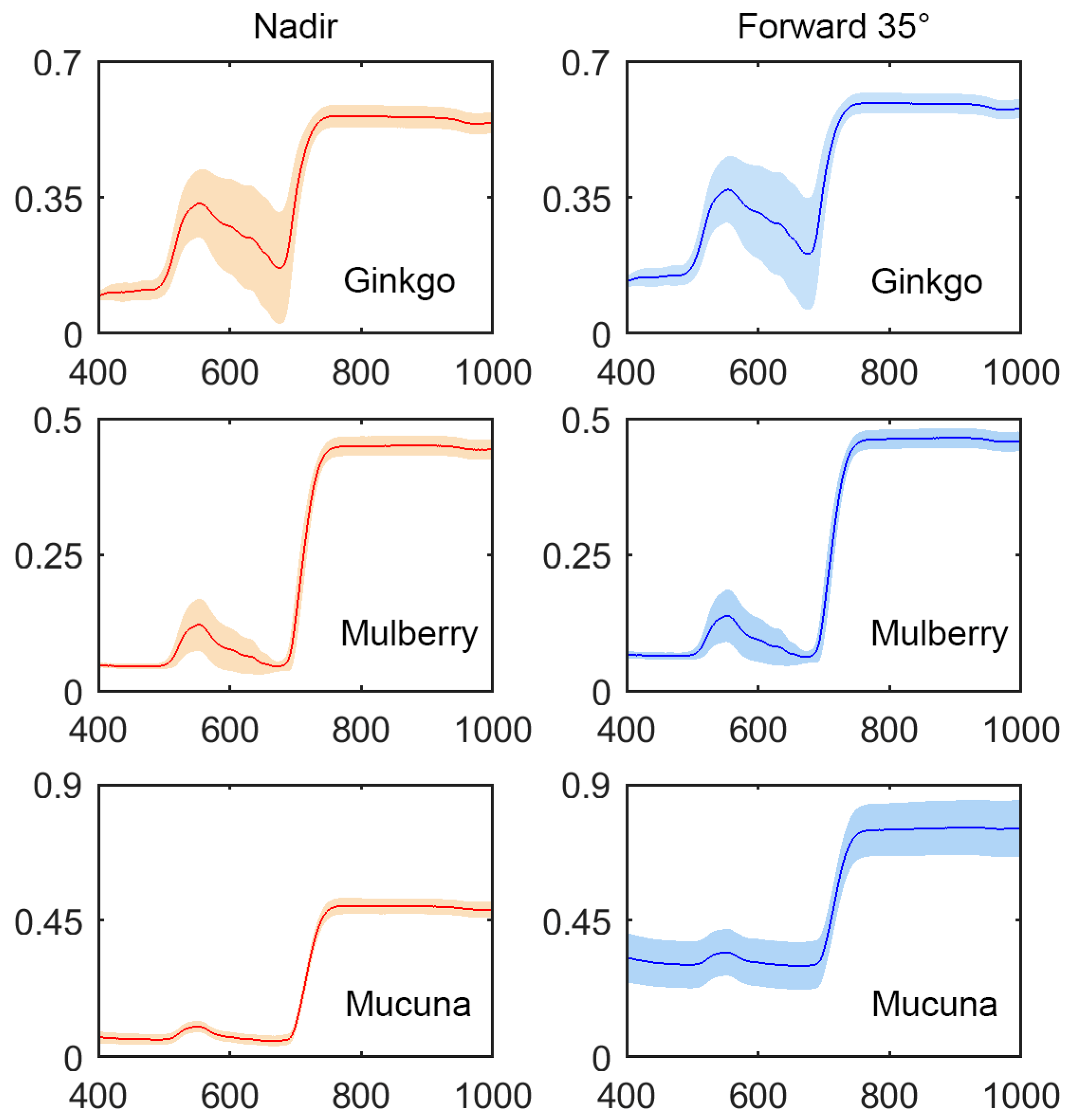
Figure 4.
The mean (solid line) ± standard deviation (colored shade) of reflectance, based on the leaf species in the nadir (first column) and forward 35° (second column) directions. The mucuna leaves have a much higher reflectance in the forward 35° than in the nadir direction.
Figure 4.
The mean (solid line) ± standard deviation (colored shade) of reflectance, based on the leaf species in the nadir (first column) and forward 35° (second column) directions. The mucuna leaves have a much higher reflectance in the forward 35° than in the nadir direction.

Figure 5.
Scatter plots for the retrievals for chlorophyll (Columns 1 and 3) and carotenoid (Columns 2 and 4) contents (μg/cm2) with PROSPECT-D (P-D) (Columns 1 and 2) and PROCOSINE (PC) (Columns 3 and 4) in the nadir (Row 1) and forward 35° (F 35°) (Row 2) directions. The x-axis is the predicted content, and the y-axis is the measured content. The retrieval is ill-posed (see Section 3.3.1). With PROSPECT-D, the mucuna leaves seriously deviate from the 1:1 line.

Figure 6.
RE for the empirical methods. The first 11 are the VIs, and the last four are the MLR-based methods. On the x-axis, except for SIPI and CWT, the remaining abbreviations indicate R-reSR, MSC+R-reSR, R-reND, SNV+R-reND, Datt_710, mSR705, mND705, Rdiff-reSR, Rdiff-reND, four-band RRDI, No processing, Derivative, and Derivative + CWT, respectively. CWT and DCWT used the underlined scales in Table 9.

Figure 7.
Correlogram for reflectance (green), first derivatives (blue), and wavelet coefficients (red, scale 8 with reflectance input, see Table 9) vs. chlorophyll content in the forward 35° direction.
Figure 7.
Correlogram for reflectance (green), first derivatives (blue), and wavelet coefficients (red, scale 8 with reflectance input, see Table 9) vs. chlorophyll content in the forward 35° direction.

Figure 8.
Correlogram between the wavelet coefficients and the carotenoid content, with the first derivative as the input. The underlined scale was the second-best for carotenoid content retrieval in the forward 35° direction (see Table 9).
Figure 8.
Correlogram between the wavelet coefficients and the carotenoid content, with the first derivative as the input. The underlined scale was the second-best for carotenoid content retrieval in the forward 35° direction (see Table 9).

Figure 9.
(a) Reflectance, (b) the first derivatives, and (c,d) wavelet coefficients using the derivative input (scales 2, 128), for the mulberry leaf in Figure 3 (chlorophyll content = 15.15 μg/cm2) in the forward 35° direction. The x-axis in each subplot is the wavelength (nm).
Figure 9.
(a) Reflectance, (b) the first derivatives, and (c,d) wavelet coefficients using the derivative input (scales 2, 128), for the mulberry leaf in Figure 3 (chlorophyll content = 15.15 μg/cm2) in the forward 35° direction. The x-axis in each subplot is the wavelength (nm).

Table 1.
Some retrieval approaches that specifically consider the specular reflectance or specular effect.
Table 1.
Some retrieval approaches that specifically consider the specular reflectance or specular effect.
| Type | Name | Formula | Specular Estimator | Reference |
|---|---|---|---|---|
| VIs | SIPI | [20] | ||
| Datt_710 | [21] | |||
| mSR705 | R445 | [17] | ||
| mND705 | R445 | [17] | ||
| R-reSR 1 | [11,15] | |||
| Rdiff-reSR | Specular reflectance | [15] | ||
| MSC+R-reSR | R-reSR using MSC processed spectrum | [11,23] | ||
| R-reND 1 | [11,15] | |||
| Rdiff-reND | Specular reflectance | [15] | ||
| SNV+ R-reND | R-reND using SNV processed spectrum | [11,27] | ||
| Four-band RRDI | (h ≠ i ≠ j ≠ k) | [24] | ||
| RT model | PROSPECT 1 | [50] | ||
| PROCOSINE | PROSPECT + simplified COSINE | bspec | [18] | |
| Hybrid model | PROCWT | PROSPECT + CWT | [25] | |
| PROSPECT + R−445 | R445 | [17,25] | ||
| PROSPECT + Rdiff + R−445 | Specular reflectance and R445 | this study |
1 These do not specifically consider the specular reflectance or specular effect and are just included for comparison.
Table 2.
Parameters, their bounds, and the initial values for optimization.
| Parameter | Lower Bound | Upper Bound | Initial Value |
|---|---|---|---|
| N (unitless) | 1 | 3 | 2 |
| Cab (chlorophylls; μg/cm2) | 0 | 100 | 16 |
| Cxc (carotenoids; μg/cm2) | 0 | 20 | 5 |
| Cw (cm) | 0.01 | 0.05 | 0.03 |
| Cm (g/cm2) | 0.002 | 0.03 | 0.01 |
| bspec (unitless) 1 | −0.9 | 0.9 | 0 |
1 Only in PROCOSINE.
Table 3.
Descriptive statistics for chlorophyll and carotenoid contents (μg/cm2).
| Species | Pigment | Number | Mean | Range | Standard Deviation |
|---|---|---|---|---|---|
| Ginkgo | Chlorophylls | 34 | 15.87 | 0.85–33.40 | 9.25 |
| Carotenoids | 4.46 | 1.58–6.96 | 1.39 | ||
| Mulberry | Chlorophylls | 20 | 36.74 | 7.57–62.48 | 14.64 |
| Carotenoids | 9.66 | 5.73–14.21 | 2.38 | ||
| Mucuna | Chlorophylls | 14 | 68.79 | 56.17–85.19 | 7.58 |
| Carotenoids | 12.38 | 10.74–14.79 | 1.32 | ||
| Total | Chlorophylls | 68 | 32.9 | 0.85–85.19 | 23.12 |
| Carotenoids | 7.62 | 1.58–14.79 | 3.74 |
Table 4.
Specular reflectance for the three leaves in Figure 3 at specific wavelengths 1.
Table 4.
Specular reflectance for the three leaves in Figure 3 at specific wavelengths 1.
| Leaf | Wavelength (nm; nadir) | Wavelength (nm; forward 35°) | ||||
|---|---|---|---|---|---|---|
| 550 | 675 | 800 | 550 | 675 | 800 | |
| Ginkgo | 0.071 | 0.059 | 0.048 | 0.094 | 0.090 | 0.085 |
| Mulberry | 0.040 | 0.036 | 0.029 | 0.047 | 0.047 | 0.039 |
| Mucuna | 0.036 | 0.031 | 0.022 | 0.308 | 0.308 | 0.282 |
Table 5.
Pigment content retrieval using the RT and hybrid models. All R2 values have a p-value < 0.01.
Table 5.
Pigment content retrieval using the RT and hybrid models. All R2 values have a p-value < 0.01.
| Direction | Pigment | Indicator | P-D 1 | P-D+Rdiff + R−445 1 | PROCWT 2 | P-D+R−445 1 | PROCOSINE |
|---|---|---|---|---|---|---|---|
| Nadir | Chlorophylls | RMSE | 6.44 | 6.22 | 5.14 | 5.23 | 5.14 |
| RE | 19.57% | 18.91% | 15.62% | 15.90% | 15.62% | ||
| R2 | 0.93 | 0.95 | 0.96 | 0.96 | 0.96 | ||
| Carotenoids | RMSE | 5.19 | 5.75 | 4.48 | 5.60 | 5.55 | |
| RE | 68.11% | 75.46% | 58.79% | 73.49% | 72.83% | ||
| R2 | 0.94 | 0.94 | 0.89 | 0.93 | 0.93 | ||
| Forward 35° | Chlorophylls | RMSE | 26.45 | 6.81 | 11.67 | 5.32 | 4.95 |
| RE | 80.40% | 20.70% | 35.47% | 16.17% | 15.05% | ||
| R2 | 0.09 3 | 0.93 | 0.97 | 0.98 | 0.97 | ||
| Carotenoids | RMSE | 6.25 | 5.69 | 5.06 | 5.55 | 5.47 | |
| RE | 82.02% | 74.67% | 66.40% | 72.83% | 71.78% | ||
| R2 | 0.11 | 0.93 | 0.85 | 0.94 | 0.94 |
1 P-D represents PROSPECT-D; 2 in the nadir direction, the scale was 32 and 8 for chlorophylls and carotenoids, respectively; in the forward 35° direction, it was 32 and 8 as well; 3 p-value = 0.012.
Table 6.
Pigment content (μg/cm2) prediction with the eight VIs.
| Direction | Pigment | Indicator | R-reSR | MSC+ R-reSR | R-reND | SNV+ R-reND | SIPI | Datt_710 | mSR705 | mND705 | Rdiff-reSR | Rdiff-reND | Four-Band RRDI 1 |
|---|---|---|---|---|---|---|---|---|---|---|---|---|---|
| Nadir | Chlorophylls | RMSE | 5.74 | 5.44 | 6.86 | 4.98 | 21.41 | 10.18 | 5.15 | 7.27 | 4.53 | 6.36 | 4.17 |
| RE | 17.45% | 16.53% | 20.85% | 15.14% | 65.08% | 30.94% | 15.65% | 22.10% | 13.77% | 19.33% | 12.67% | ||
| R2 | 0.94 | 0.95 | 0.92 | 0.96 | 0.26 | 0.83 | 0.95 | 0.91 | 0.96 | 0.93 | 0.97 | ||
| p-value | <0.01 | <0.01 | <0.01 | <0.01 | 0.39 | <0.01 | <0.01 | <0.01 | <0.01 | <0.01 | <0.01 | ||
| Carotenoids | RMSE | 0.93 | 0.99 | 0.96 | 0.98 | 3.39 | 1.60 | 1.06 | 1.08 | 0.92 | 0.97 | 0.80 | |
| RE | 12.20% | 12.99% | 12.60% | 12.86% | 44.49% | 21.00% | 13.91% | 14.17% | 12.07% | 12.73% | 10.50% | ||
| R2 | 0.94 | 0.93 | 0.94 | 0.93 | 0.26 | 0.84 | 0.92 | 0.92 | 0.94 | 0.93 | 0.95 | ||
| p-value | <0.01 | <0.01 | <0.01 | <0.01 | 0.05 | <0.01 | <0.01 | <0.01 | <0.01 | <0.01 | <0.01 | ||
| Forward 35° | Chlorophylls | RMSE | 17.47 | 6.25 | 15.93 | 4.82 | 21.40 | 8.80 | 6.62 | 7.41 | 6.25 | 7.43 | 4.25 |
| RE | 53.10% | 19.00% | 48.42% | 14.65% | 65.05% | 26.75% | 20.12% | 22.52% | 19.00% | 22.58% | 12.92% | ||
| R2 | 0.49 | 0.93 | 0.55 | 0.96 | 0.26 | 0.87 | 0.94 | 0.91 | 0.93 | 0.90 | 0.97 | ||
| p-value | <0.01 | <0.01 | <0.01 | <0.01 | 0.04 | <0.01 | <0.01 | <0.01 | <0.01 | <0.01 | <0.01 | ||
| Carotenoids | RMSE | 2.27 | 1.00 | 2.07 | 0.94 | 3.39 | 1.33 | 1.18 | 1.06 | 0.99 | 1.07 | 0.90 | |
| RE | 29.79% | 13.12% | 27.17% | 12.34% | 44.49% | 17.45% | 15.49% | 13.91% | 12.99% | 14.04% | 11.81% | ||
| R2 | 0.63 | 0.93 | 0.68 | 0.94 | 0.25 | 0.88 | 0.91 | 0.92 | 0.93 | 0.92 | 0.94 | ||
| p-value | <0.01 | <0.01 | <0.01 | <0.01 | 0.04 | <0.01 | <0.01 | <0.01 | <0.01 | <0.01 | <0.01 |
1 In the nadir direction, this was and for chlorophylls and carotenoids, respectively; in the forward 35° direction, it was and .
Table 7.
Pigment content (μg/cm2) prediction using MLR for the original reflectance. All R2 values have a p-value < 0.01.
Table 7.
Pigment content (μg/cm2) prediction using MLR for the original reflectance. All R2 values have a p-value < 0.01.
| Pigment | Direction | Wavelength (nm) | RMSE | RE | R2 | ||
|---|---|---|---|---|---|---|---|
| Chlorophylls | Nadir | 710 | 725 | 772 | 3.14 | 9.54% | 0.98 |
| Forward 35° | 400 | 713 | 780 | 4.24 | 12.89% | 0.97 | |
| Carotenoids | Nadir | 714 | 769 | – | 1.10 | 14.44% | 0.92 |
| Forward 35° | 439 | 705 | – | 1.15 | 15.09% | 0.91 | |
Table 8.
Pigment content (μg/cm2) prediction using MLR for the first derivatives. All R2 values have a p-value < 0.01.
Table 8.
Pigment content (μg/cm2) prediction using MLR for the first derivatives. All R2 values have a p-value < 0.01.
| Pigment | Direction | Wavelength (nm) | RMSE | RE | R2 | ||
|---|---|---|---|---|---|---|---|
| Chlorophylls | Nadir | 576 | 745 | 778 | 2.72 | 8.27% | 0.99 |
| Forward 35° | 474 | 747 | 773 | 2.63 | 7.99% | 0.99 | |
| Carotenoids | Nadir | 752 | 955 | – | 0.96 | 12.60% | 0.94 |
| Forward 35° | 736 | 949 | – | 0.92 | 12.07% | 0.94 | |
Table 9.
Pigment content (μg/cm2) prediction with the CWT plus MLR method. The “spectral input type” is the spectrum type that is used for the wavelet transformation. The underlined results are the best (the second-best for carotenoids in the forward 35° direction) for a pigment in a direction, among all of the retrieval methods. All R2 values have a p-value < 0.01.
| Direction | Spectral input Type | Pigment | Optimal Scale | Wavelength (nm) | RMSE | RE | R2 | ||
|---|---|---|---|---|---|---|---|---|---|
| Nadir | Original reflectance | Chlorophylls | 8 | 568 | 708 | 764 | 2.68 | 8.15% | 0.99 |
| Carotenoids | 4 | 750 | 1000 | – | 0.88 | 11.55% | 0.95 | ||
| First derivative | Chlorophylls | 8 | 580 | 771 | 786 | 2.80 | 8.51% | 0.99 | |
| Carotenoids | 16 | 556 | 783 | – | 0.90 | 11.81% | 0.95 | ||
| Forward 35° | Original reflectance | Chlorophylls | 8 | 580 | 761 | 862 | 2.42 | 7.36% | 0.99 |
| Carotenoids | 16 | 536 | 775 | – | 0.88 | 11.55% | 0.95 | ||
| First derivative | Chlorophylls | 8 | 732 | 767 | 782 | 2.74 | 8.32% | 0.99 | |
| Carotenoids | 64 | 472 | 776 | – | 0.86 1 | 11.29% | 0.95 | ||
1 The second-best, and only slightly higher than 0.80 from the four-band RRDI in Table 6.
Table 10.
The MLR retrieval models for the original reflectance. The wavelengths correspond to the ones in Table 7, in sequence.
Table 10.
The MLR retrieval models for the original reflectance. The wavelengths correspond to the ones in Table 7, in sequence.
| Direction | Pigment | Wavelength Coefficients | Constant Term | ||
|---|---|---|---|---|---|
| Nadir | Chlorophylls | 148.91 | −748.51 | 598.50 | 3.09 |
| Carotenoids | −37.04 | 19.89 | — | 10.77 | |
| Forward 35° | Chlorophylls | 113.73 | −220.83 | 158.02 | 16.56 |
| Carotenoids | 36.27 | −31.12 | — | 13.09 | |
© 2019 by the authors. Licensee MDPI, Basel, Switzerland. This article is an open access article distributed under the terms and conditions of the Creative Commons Attribution (CC BY) license (http://creativecommons.org/licenses/by/4.0/).
Share and Cite
MDPI and ACS Style
Li, Y.; Huang, J. Remote Sensing of Pigment Content at a Leaf Scale: Comparison among Some Specular Removal and Specular Resistance Methods. Remote Sens. 2019, 11, 983. https://0-doi-org.brum.beds.ac.uk/10.3390/rs11080983
AMA Style
Li Y, Huang J. Remote Sensing of Pigment Content at a Leaf Scale: Comparison among Some Specular Removal and Specular Resistance Methods. Remote Sensing. 2019; 11(8):983. https://0-doi-org.brum.beds.ac.uk/10.3390/rs11080983
Chicago/Turabian StyleLi, Yingying, and Jingfeng Huang. 2019. "Remote Sensing of Pigment Content at a Leaf Scale: Comparison among Some Specular Removal and Specular Resistance Methods" Remote Sensing 11, no. 8: 983. https://0-doi-org.brum.beds.ac.uk/10.3390/rs11080983
Note that from the first issue of 2016, this journal uses article numbers instead of page numbers. See further details here.