Assessment of Different Stochastic Models for Inter-System Bias between GPS and BDS


1
Institute of Space Sciences, Shandong University, Weihai 264209, China
2
Institut für Geodäsie und Geoinformationstechnik, Technical University of Berlin, 10623 Berlin, Germany
3
German Research Centre for Geosciences GFZ, Telegrafenberg, 14473 Potsdam, Germany
4
State Key Laboratory of Geo-Information Engineering, Xi’an 710054, China
*
Author to whom correspondence should be addressed.
Remote Sens. 2019, 11(8), 989; https://0-doi-org.brum.beds.ac.uk/10.3390/rs11080989
Submission received: 15 March 2019
/
Revised: 19 April 2019
/
Accepted: 23 April 2019
/
Published: 25 April 2019
(This article belongs to the Special Issue Global Navigation Satellite Systems for Earth Observing System)
Abstract
:Inter-system bias (ISB) will affect accuracy and processing time in integrated precise point positioning (PPP), and ISB stochastic models will largely determine the quality of ISB estimation. Thus, the impacts of four different stochastic models of ISB processing will be assessed and studied in detail to further reveal the influence of ISB in positioning. They are ISB-PW considering ISB as a piece-wise constant, ISB-RW considering ISB as random walk, ISB-AD considering ISB as an arc-dependent constant, and ISB-WN considering ISB as white noise. Together with the model without introducing ISB called ISB-OFF, i.e., five different schemes, ISB-OFF, ISB-PW, ISB-RW, ISB-AD, and ISB-WN, will be designed and tested in this study. From the results of pseudorange residuals, it can be noticed that when considering ISB, the Root-Mean-Square (RMS) of ionosphere-free combined pseudorange residuals are much smaller than without ISB (ISB-OFF). The results of convergence time and positioning accuracy analysis show that PPP performance with ISB-AD is even worse than ISB-OFF, when using the precise products from the German Research Centre for Geosciences (GFZ) named as GBM products here; while the strategies of ISB-RW, and ISB-WN achieve the best results. For the products from Wuhan University called WUM products, a completely different result is achieved. PPP with the stochastic models of ISB-PW and ISB-AD perform best. The most likely reason is the ISB stochastic models applied by the analysis centers are consistent with those used in the PPP on the user side. So, ISB-RW, or ISB-WN is recommended when GBM products are used, and for the WUM products, ISB-PW, or ISB-AD is chosen. From the statistics of PPP precision during the convergence period, it can be concluded that considering ISB also has a great improvement on combined PPP accuracy during the initialization phase.
1. Introduction
Along with the modernization of the Global Positioning System (GPS) [1], the revitalization of the Russian Global Navigation Satellite System (GLONASS) [2], the launch of more European Global Navigation Satellite System (Galileo) satellites [3], and the fast development of Chinese BeiDou Navigation Satellite System (BDS) [4,5], more and more satellites can be observed at one place. Together with the initiation of the Multi-GNSS Experiment (MGEX) in 2012 [6], precise point positioning (PPP) has been stepped up into the stage of multi-system combined mode. However, because of different time systems, reference frames, and hardware delays within receivers used in different systems [7,8], biases exist between different systems when we are making multi-GNSS combined PPP. If we blindly apply observations from all systems without any calibration of these biases, a poor accuracy result will be achieved, and sometimes even worse than that of the single-system PPP. Hence, biases between different systems need to be carefully considered and calibrated, which is the basis of multi-system integrated positioning. Often, an extra parameter named inter-system bias (ISB) is introduced to cover the biases between different satellite systems [9,10,11]. Currently, the processing strategy for ISB is usually to estimate it together with other unknown items, such as coordination, receiver clock, and tropospheric delay, etc. As for the estimation stochastic models of ISB, normally a strategy of considering ISB as an arc-dependent constant is applied in Paziewski and Wielgosz [12], Li, et al. [13], Guo, et al. [14], and Lou, et al. [15]. Besides applying the code ISB estimation, the stochastic model of considering ISB as an arc-dependent constant is also used in the phase ISB estimation for PPP ambiguity resolution (PPP-AR). Because day-to-day variation of phase ISB is less than 0.1 cycles, the phase ISB is usually estimated as an arc-dependent constant every 24 h [16,17]. Jiang, et al. [9] regard ISB as a piece-wise parameter, which can increase the sample size and is good for ISB modeling and prediction. Besides these two strategies, another two stochastic models can be used, which are considering ISB as white noise or as random walk. However, up to now, no specific analysis has been made to assess the difference between these stochastic models and their impact on ISB estimation, therefore in this study, we will evaluate and compare the influence of different stochastic models on ISB, positioning accuracy, and processing time. Based on the results, the recommendations on the selections for the ISB stochastic models will be given.
The paper is organized as follows: Section 2 gives the introductions on the PPP model for ISB estimation and processing strategies. In addition, the detailed descriptions of four different ISB stochastic models and five designed schemes are made. Then, the experimental data used in this study are declared in Section 3. The results and analysis are shown in Section 4, inside pseudorange observation residuals. The estimated ISBs, convergence time, positioning accuracy with GBM and WUM precise products, and accuracy improvement during the convergence time are discussed and compared with five different strategies. Finally, conclusions of this study are made in Section 5.
2. Model for Inter-System Bias Estimation and Descriptions of the Stochastic Models
The main biases between two satellite systems are related to the satellite constellations, the signals broadcast, and time and coordinate frame conventions [18]. Thus, in our multi-GNSS combined processing model, we introduce an extra ISB parameter to cover the effect of the biases between the two systems, and the ISB is estimated with other unknowns using the ionospheric-free (IF) PPP processing.
2.1. Model for Inter-System Bias Estimation and Processing Strategies
The ionosphere-free (IF) pseudorange and phase observation functions between the receiver and a satellite can be written as:
where , are pseudorange and carrier-phase IF combined observations, respectively; is the range between the receiver and the satellite; is the light speed; is the receiver clock error and is the satellite clock error; and are mapping function and zenith tropospheric delay; the first-order error of ionospheric delay is eliminated by ionosphere-free combination; , and , are the pseudorange and carrier-phase hardware delay biases of the ionospheric-free function for receivers and satellites; is ambiguity in distance; and denote unmodeled parameters (e.g., the measurement noise and multipath errors for pseudorange and carrier phase).
The pseudorange hardware delay biases , in the GNSS observations can be assimilated into the clock errors . The carrier-phase hardware delay biases , are not considered in most GNSS data processing, since the carrier-phase hardware delay biases is satellite dependent and stable over time; thus, it can be absorbed by the ambiguity [19,20]. Using the precise satellite orbit and clock products, Equation 1 can be rewritten as:
where and are redefined receiver clock error and ambiguity:
Because the satellite hardware delays are contained in the precise satellite clock and can be eliminated on the user side when applying the precise products in Equation (2) [21]. In Equation (3), the ambiguity term is not an integer property anymore since it contains the bias term, which is the uncalibrated hardware delay biases, showing a fractional cycle property. Thus, the term is called the uncalibrated phase delay [22].
The tight combined PPP model requires the estimation of an extra ISB parameter. Hence, the combined observation model can be expressed as:
where in the notation of the receiver clock error, mapping functions, the ambiguity, and some other parameters, we use the superscript G as GPS to distinguish them from the parameters of other systems, which are denoted with the superscript O. is a common item between different systems, being the receiver clock term relating to the GPS. The is the inter-system bias parameter between GPS and other systems in the unit of time. It will be modeled as an unknown parameter and estimated together with the other parameters such as coordinates and the receiver clock error. So, the corresponding estimated parameters vector is,
where denotes the vector of the receiver position increments, and are the modified ambiguity parameters for different systems. Here, we take GPS and BDS systems as an example for data processing, and a Kalman filter is employed to estimate the unknown parameters in the processing [23,24,25].
Suppose the initial state value is , the variance is , so the state estimation at epoch can be obtained recursively by Kalman filter:
- (a)
- One-step state prediction:
- (b)
- One-step prediction of covariance:
- (c)
- Filtering gain:
- (d)
- Status update:
- (e)
- State covariance update:where is transition matrix; is the coefficient matrix of observation equation; and is the variance matrix of system noise sequence and variance matrix of observation noise, respectively; and is one-step prediction value and its variance-covariance matrix, respectively; is gain matrix; and is filtered estimation and its variance-covariance matrix, respectively; denotes the unit matrix.
In this experiment, during the preprocessing we detect and repair clock jumps to avoid misidentifying an observation jump caused by the receiver clock jumps as the cycle slip. Afterwards, the Geometry-Free (GF) and Hatch-Melbourne-Wubbena (HMW) [26,27,28] combinations are used to detect cycle slips. The previously described Kalman filter is employed to estimate the unknown parameters with a sliding window of 3 h station by station, which means the 24-h observation data for each station will be divided into 8 processing sessions. GPS and BDS combined PPP in static and simulated kinematic modes are applied in our study. In static PPP mode, the solution strategy for position coordinates is to consider as contents, while for the kinematic PPP mode, they are estimated as white noise at each epoch. To analyze the impacts of different precise products from different analysis centers (AC) on the ISB estimation, the MGEX precise products from two ACs, GFZ (GBM) and Wuhan University (WUM) are used to fix the satellite orbit and clock in the combined PPP model.
The dry component of the tropospheric delay is corrected with the Saastamoinen model, while the residual zenith wet delay is estimated as a random-walk process. We apply the Global Mapping Function (GMF) [29] to convert zenith delay to slant directions. The cutoff elevation angle is set as 7° and an elevation-dependent weighting method is used. Moreover, the phase-wind up effects [30], the solid earth tide, the ocean loading tide [31] and relativistic effects are corrected by the model. Up to now, BDS-specific receiver antenna Phase Center Offsets (PCOs) and Phase Center Variations (PCVs) are not provided in the igs14.atx. In this case, GPS-specific receiver PCOs and PCVs are applied instead. The initial standard deviation for the carrier-phase observations in GPS and BDS systems are set to 0.003 m, while that for the pseudorange observations is set to 0.3 m. The details of models and strategies related to the data processing are listed in Table 1.
The estimation of the ISB parameter can be performed with different stochastic models, such as white noise, random walk, piece-wise constant, or processing-arc-dependent constant, which will be discussed and studied in detail in the following.
2.2. The Different Stochastic Models
To not only verify the importance of ISB, and its influence on the accuracy of tight combined PPP model, but also compare the impacts of different ISB estimation stochastic models on the positioning, five different schemes are proposed in this study. The differences between different schemes mainly focus on the configurations on the ISB. Here, we will take one 3-h processing-arc-window containing 360 observation epochs as an example.
- Neglecting inter-system bias between GPS and BDS is named ISB-OFF, which means the positioning model of BDS and GPS is separated, and the two systems are processed without any relation. The BDS observations are processed the same as GPS ones. However, the ISB between GPS and BDS will remain in the BDS processing model and will be reflected in the pseudorange residuals. The configuration equation can be expressed as:where is the ISB in the scheme ISB-OFF. to is an empty matrix which means without considering ISB.
- Estimating the ISB as a piece-wise constant every 30 min (ISB-PW). ISB parameter is initialized at the first epoch, then re-initialized, and updated every 30 min [9]. The configuration equation can be written as:where means the ISB in the scheme ISB-PW. The ISB in one 3-h processing-arc-window can be divided into six parts according to size of piece-wise (every 30 min), which are denoted as to . is one piece-wise ISB, and is from 1 to 6.
- Estimating the ISB as a random-walk processing (ISB-RW). With this scheme, ISB is initialized at the first epoch, and then with a time-related spectral density of 0.001 . The configuration equation can be formed as:where is the ISB in the scheme ISB-RW. is the ISB for one epoch, with from 1 to 360. means the time-related spectral density.
- Estimating the ISB as a processing-arc-dependent constant (ISB-AD). During the whole processing-arc period, ISB is only initialized at the first epoch. If the processing-arc window is one day, this means the ISB is estimated as a constant each day. In this paper, we make the period of our processing tests as 3 h, so the ISB is considered to be a 3-h arc-dependent constant. The configuration equation can be indicated as:where means the ISB in the scheme ISB-AD, which is estimated as a constant during the 3-h processing-arc window.
- Estimating the ISB as white noise (ISB-WN). In this way, the ISB is initialized for each epoch, which is the same as the normal processing mode as the receiver clock error. The configuration equation can be shown as:where means the ISB in the scheme ISB-WN. The ISB in each epoch will be initialized and estimated.
For convenience, the five schemes mentioned above marked as ISB-OFF, ISB-PW, ISB-RW, ISB-AD, and ISB-WN, respectively, are summarized in Table 2.
3. Experimental Data
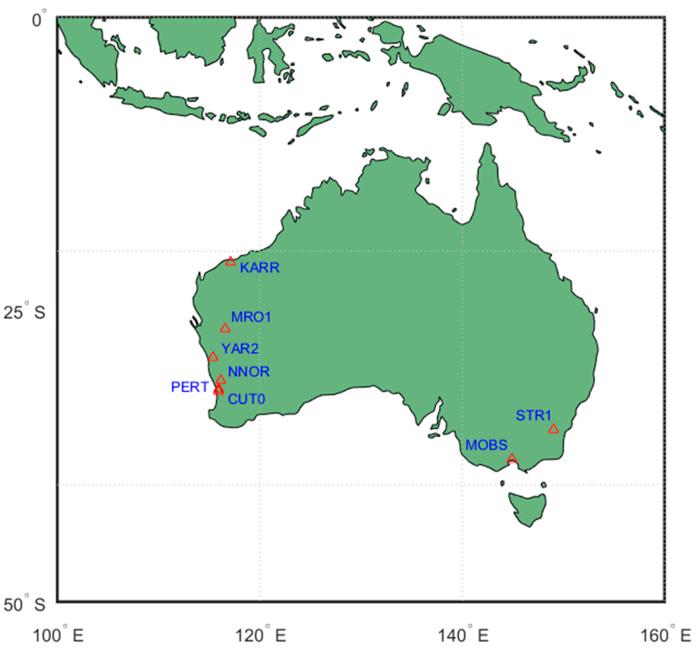
To validate the different proposed ISB estimation stochastic models and the influence of the extra parameter ISB on PPP performance, observations from 8 stations in the MGEX network, named as CUT0, KARR, MRO1, PERT, MOBS, NNOR, STR1, and YAR2, were chosen, covering a one-week period which is GPS week 1965 with the DOY (day of year) from 246-252, 2017. These 8 stations are all located in Australia, where we can usually observe more than 7 BDS satellites [5]. The distribution and the receiver types equipped in the stations are shown in Figure 1 and Table 3.
The data of these 8 stations will be processed with the tight combined PPP model, and with the different stochastic models for ISB estimation mentioned above. The results in static and kinematic mode using GBM and WUM precise products will be analyzed and explained in the following sections.
4. Results and Discussion
This section presents the results and analysis performed to assess the difference between diverse ISB stochastic models and their impacts on positioning accuracy and convergence time. As mentioned before, processing is re-initialized eight times per day to evaluate the influence on convergence time. One initialization is considered to be a cold start. A time slide window of 3 h is chosen to ensure enough time for converging into a certain accuracy in nearly all the cases and offer enough test samples. Considering the entire experiment over all stations, it gives 448 cold starts (8 stations × 7 days × 8 initializations).
Here, we use the station coordinates from the IGS weekly solutions as the references, and the positioning errors are defined as the increments between PPP results and the references. The statistical analysis of positioning errors are made with the methods of 68% and 95% quantiles. These two statistical parameters are chosen instead of mean and standard deviation due to the possible remaining biases that might cause results do not follow a normal distribution [32]. The convergence time is defined as when the positioning error is lower than 0.2 m (95%) and 0.1 m (68%) in the North, East, and UP components [15]. This statistical approach is also used in Bree and Tiberius [33], Jr, et al. [32], and Zhou, et al. [34].
Since different MGEX analysis center (GBM, or WUM) has its own processing strategy to obtain precise multi-GNSS orbit and clock products, during the product generation, different ISB stochastic models will be employed with different ACs. In this study, we will apply the precise products from GBM and WUM to validate the difference between these two kinds of products and analyze the potential influence of the different ISB estimation strategies used in different ACs on the positioning and convergence time.
4.1. Pseudorange and Carrier-Phase Observation Residuals
As is already known, the remaining measurement noises and other unmodeled errors will be assimilated by the observation residuals, which is a very important indicator to assess the accuracy of the positioning model. Thus, here the pseudorange and carrier-phase observation residuals will be assessed and compared in the five different schemes.
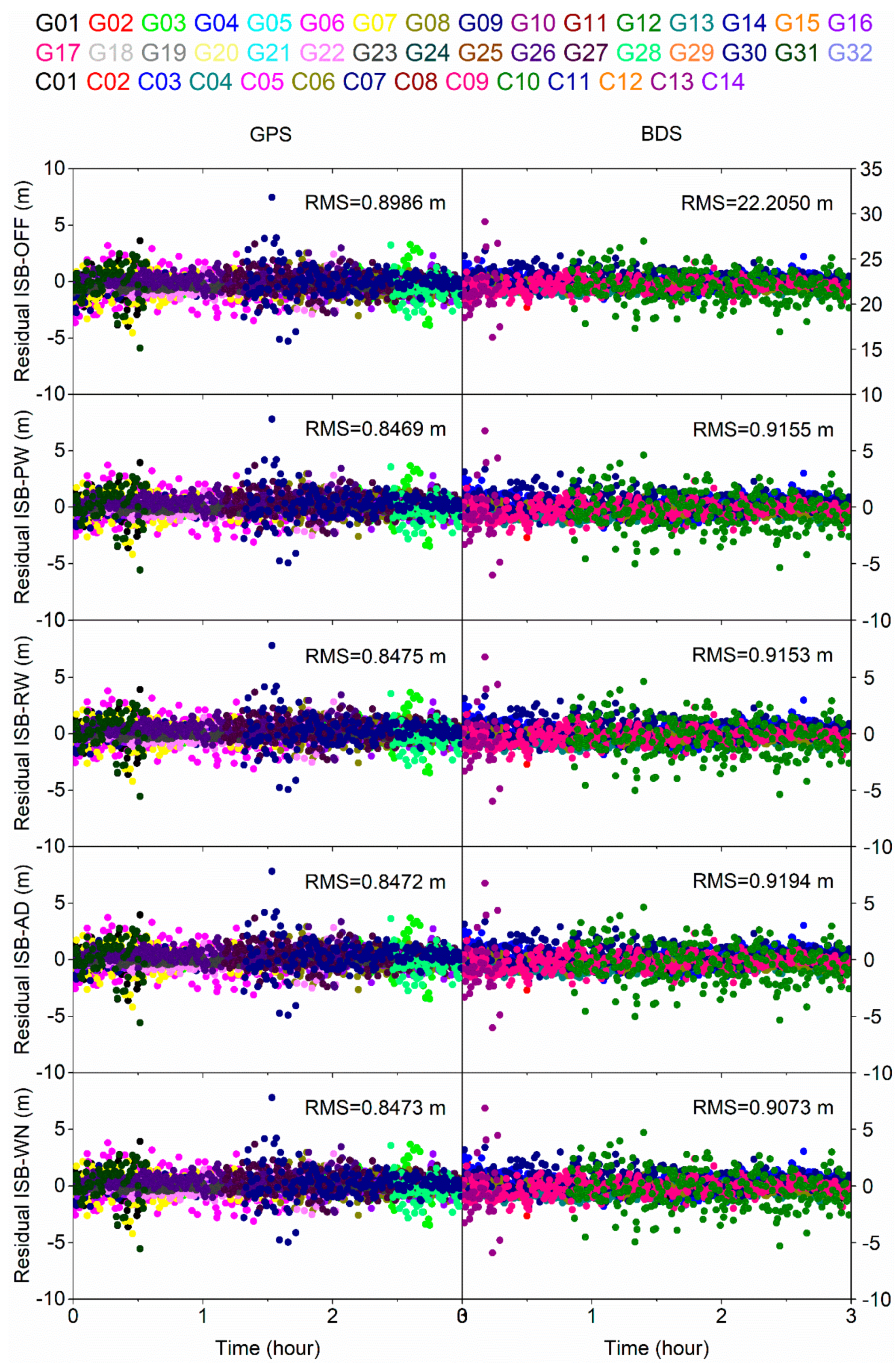
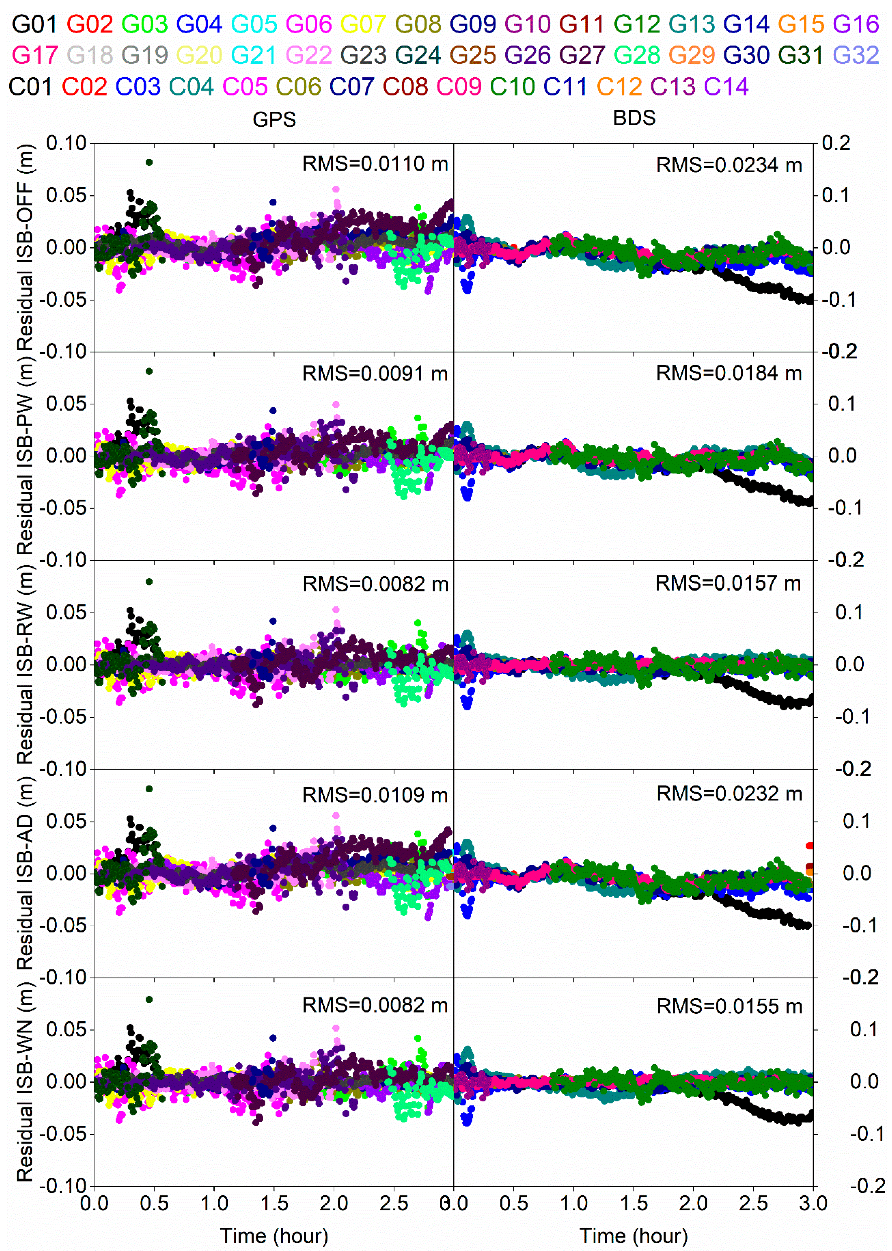
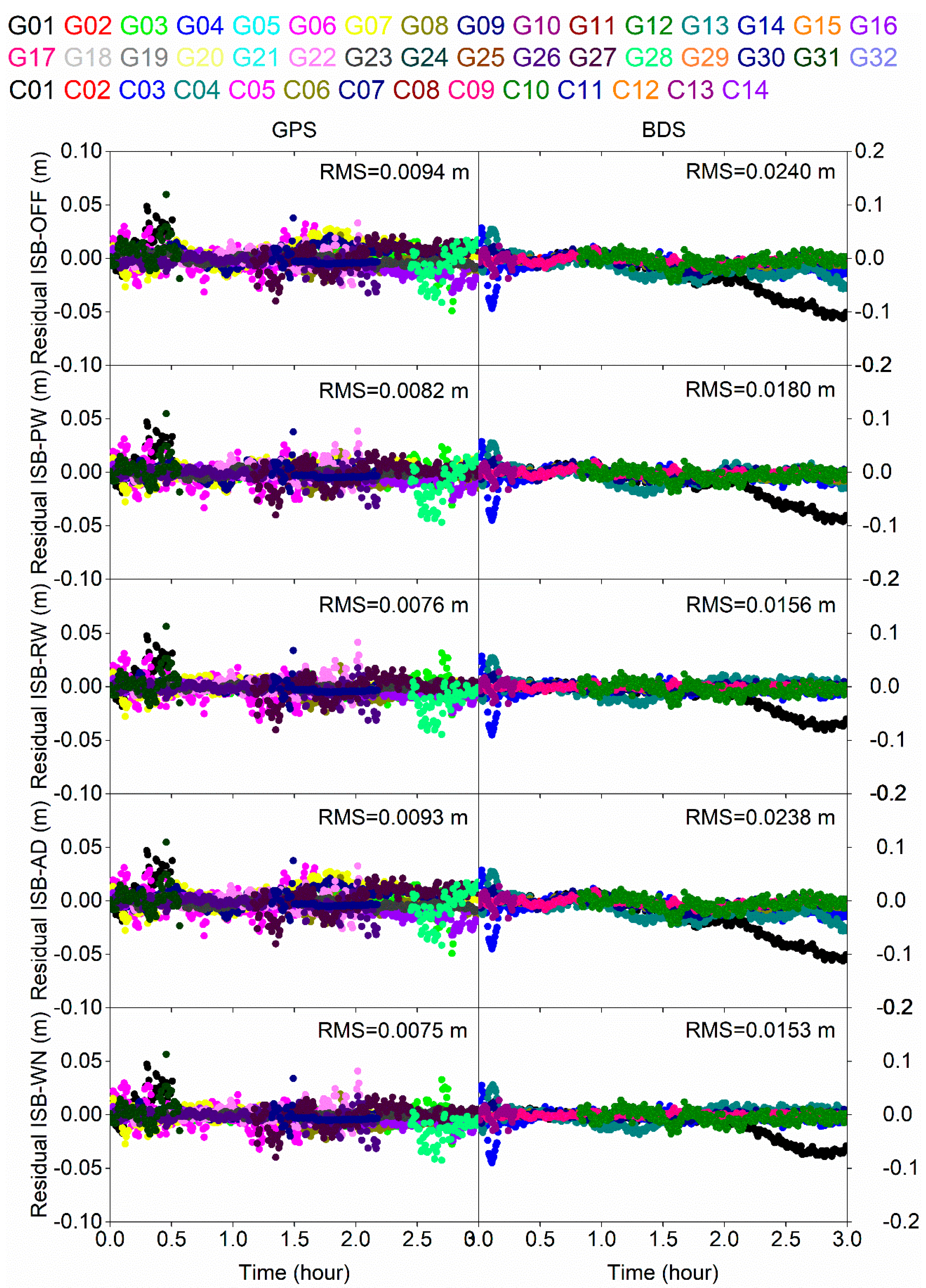
The pseudorange residuals at station STR1 (with the GBM products as an example) of each satellite with different colors in GPS and BDS system, respectively, are shown in Figure 2 and Figure 3. Figure 2 is the result of static mode, while Figure 3 is the kinematic mode. From the figures, we can see that both in the static and kinematic modes, compared to considering ISB, neglecting ISB (ISB-OFF) will lead to a higher pseudorange residual. After introducing the ISB parameter (ISB-PW, ISB-RW, ISB-AD, and ISB-WN), the ionospheric-free pseudorange (PC) residuals in GPS system will on average improve 4.8 cm (i.e., 5.4%) in static mode, and 5.1 cm (i.e., 5.7%) in kinematic mode. The improvement is not obvious, which is in accordance with the ISB processing strategy that the GPS receiver clock error is considered to be the reference clock error, and ISB covers the biases between BDS and GPS. Thus, the ISB has no effect on the pseudorange residuals in GPS system. As for the BDS system, the PC residual of ISB-OFF is largest; because the remaining errors and difference are not absorbed by ISB, they go into the residuals. The statistical results of the other four schemes are similar, and compared to ISB-OFF, the RMS of pseudorange residuals for ISB-PW, ISB-RW, ISB-AD, and ISB-WN can reduce by 21.3 m (95.9%) both in static mode and kinematic mode. Hence, we can conclude that it is necessary to consider the ISB parameter in multi-GNSS combined positioning. In addition, the carrier-phase observation residuals of GPS and BDS satellites in station STR1 with the GBM products are also taken as an example, the results of static and kinematic modes are displayed in Figure 4 and Figure 5, respectively.
It can be noted from Figure 4 and Figure 5 that the RMS of carrier-phase observation residuals is two orders of magnitude lower than that of the pseudorange residuals, which is caused by the different measurement accuracy levels of pseudorange and carrier-phase observations. Compared with neglecting ISB, the RMS of carrier-phase residuals considering ISB has no significant improvement regarding the pseudorange residuals. That is because in the carrier-phase PPP performance except ISB, the ambiguity is also an unknown parameter. If the ISB is neglected, the impact of unmodeled ISB will be partly or even totally assimilated by the ambiguity, which means the effect of considering ISB or not will not obviously reflect in the carrier-phase residuals. Besides, we can see that when using GBM products, the RMS of carrier-phase residuals in ISB-RW and ISB-WN are the best. Compared with the residuals in ISB-OFF and ISB-AD, the RMS can on average improve by 25.5% and 33.8% in GPS and BDS satellites in the static mode, and for the kinematic mode the improvement rate is 20.2% and 36.3% in GPS and BDS satellites. The carrier-phase observation residuals mainly reflected the accuracy of PPP performance, so we can conclude that the ISB stochastic models impact the carrier-phase observation residuals, and will have a further influence on the PPP performance. In the following parts, the impact of ISB stochastic models on the ISB estimation and PPP performance will be studied in detail.
4.2. Comparison of Estimated Inter-System Bias
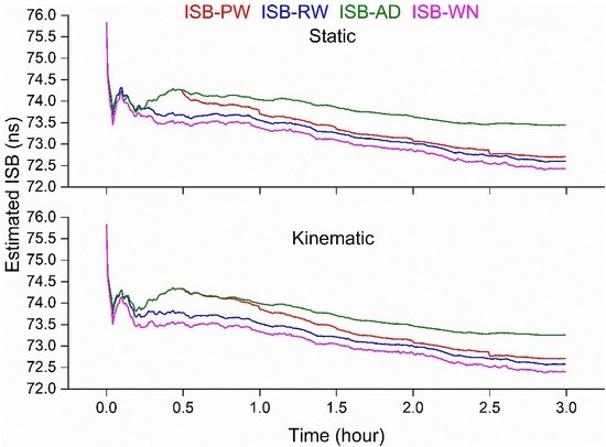
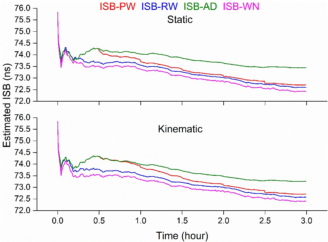
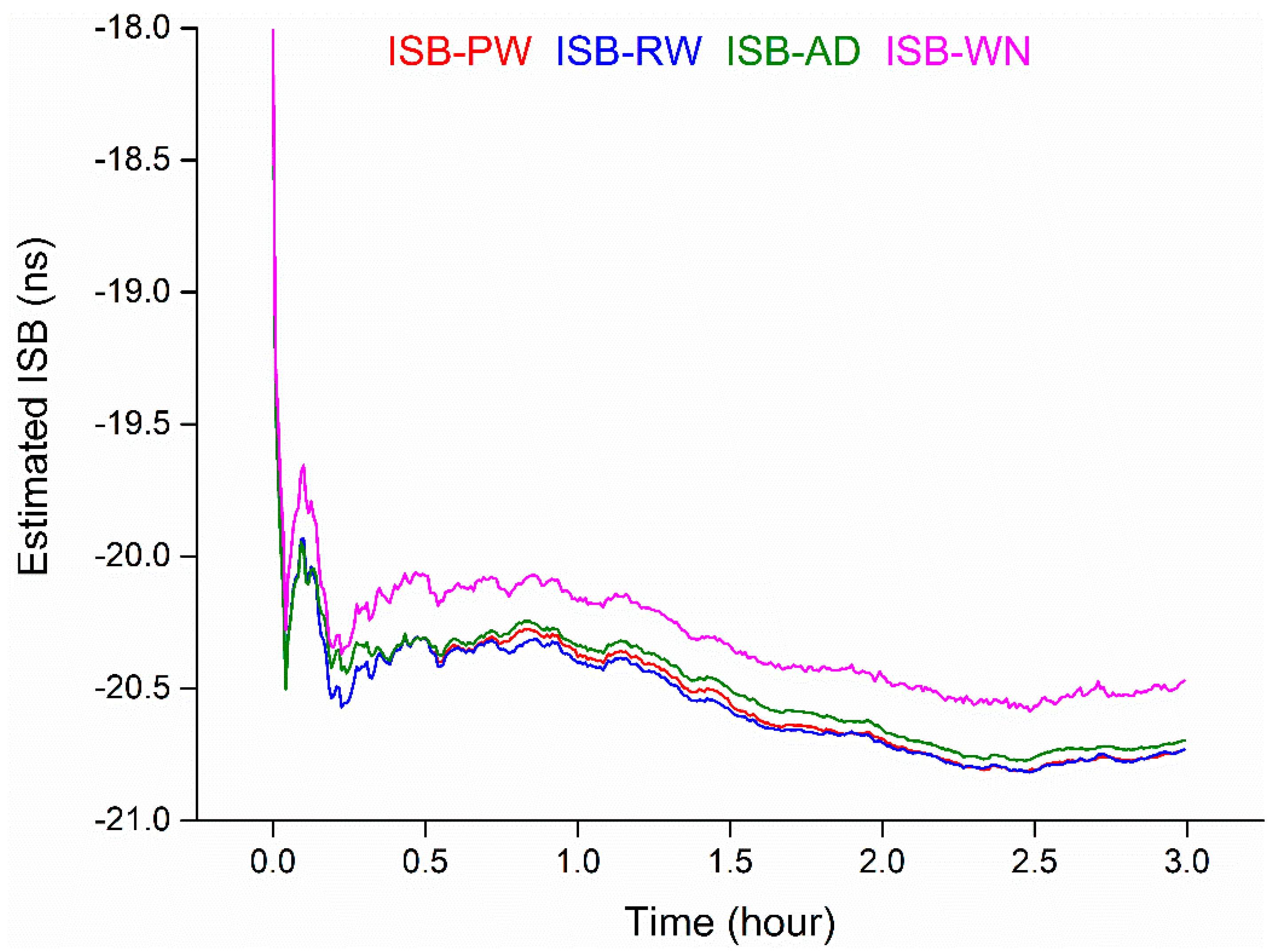
The estimated ISB is the most direct factor to reflect which the stochastic model is the optimal one for the PPP performance and how to select an ideal stochastic model for different precise products. Thus, the comparisons of the estimated ISBs from the schemes ISB-PW, ISB-RW, ISB-AD, and ISB-WN using GBM and WUM precise products are made. Figure 6 shows the estimated ISBs using the GBM products in static and kinematic modes. The first 3-h ISB results on DOY 251, 2017 in the station STR1 are taken as an example.
From Figure 6, we can see that the four estimated ISBs from PPP performance with different stochastic models using GBM products have completely different results. The ISBs in ISB-AD have the largest values. The ISBs in ISB-PW are coincident with those in ISB-AD in the first 30 min, but they show different values in the following periods because ISB in ISB-PW was initialized every 30 min. The ISBs in ISB-RW and ISB-WN demonstrate the consistent trend but with a systematic difference, which will be absorbed by the ambiguity in the PPP solution. To deeply show the feature ISBs with different precise products, PPP performance using the WUM products is made. The estimated ISBs with the WUM product is shown in Figure 7.
It can be noticed from Figure 7 that entirely different from the results in Figure 6, the ISBs in ISB-PW, ISB-RW, and ISB-AD have the same trend and very close values. A consistent trend is displayed between the ISB in ISB-WN and the other three ISBs, but the ISB in ISB-WN is rougher than others. The impacts of the different features of ISBs on PPP performance will be analyzed and assessed in the next step.
4.3. Convergence Time and Positioning Accuracy
Positioning accuracy is evaluated by comparing the coordinates with external reference values, which are from the final IGS weekly solution. As for the statistics of convergence time, we use the statistical method of 68% and 95% quantiles mentioned above. In the 68% quantile case, we make the convergence time as the first epoch time whose error is less than 0.1 m and the errors in the following epochs are all less than 0.1 m. As for the 95% quantile, the criterion is less than 0.2 m.
4.3.1. The Case with GBM Precise Products
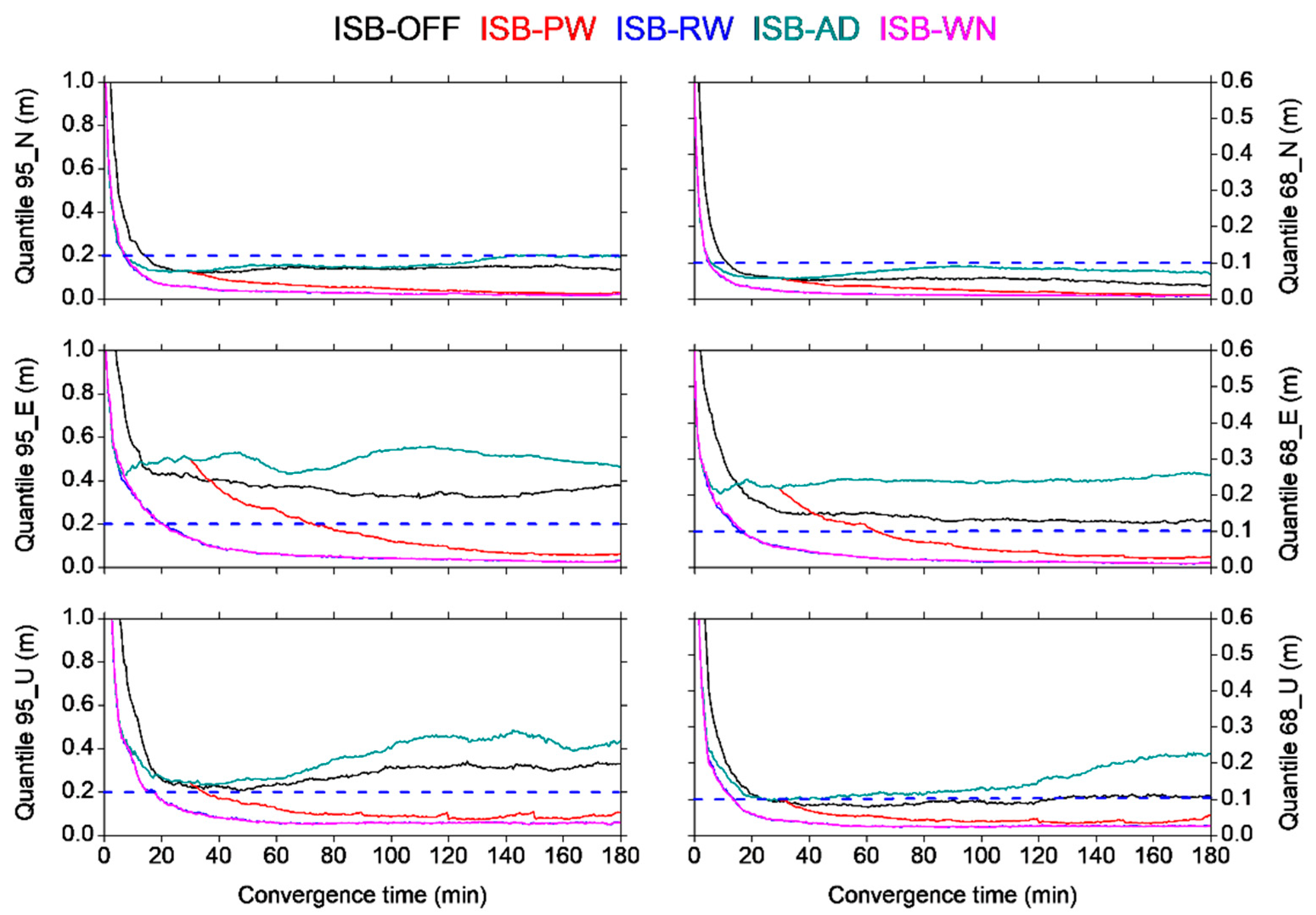
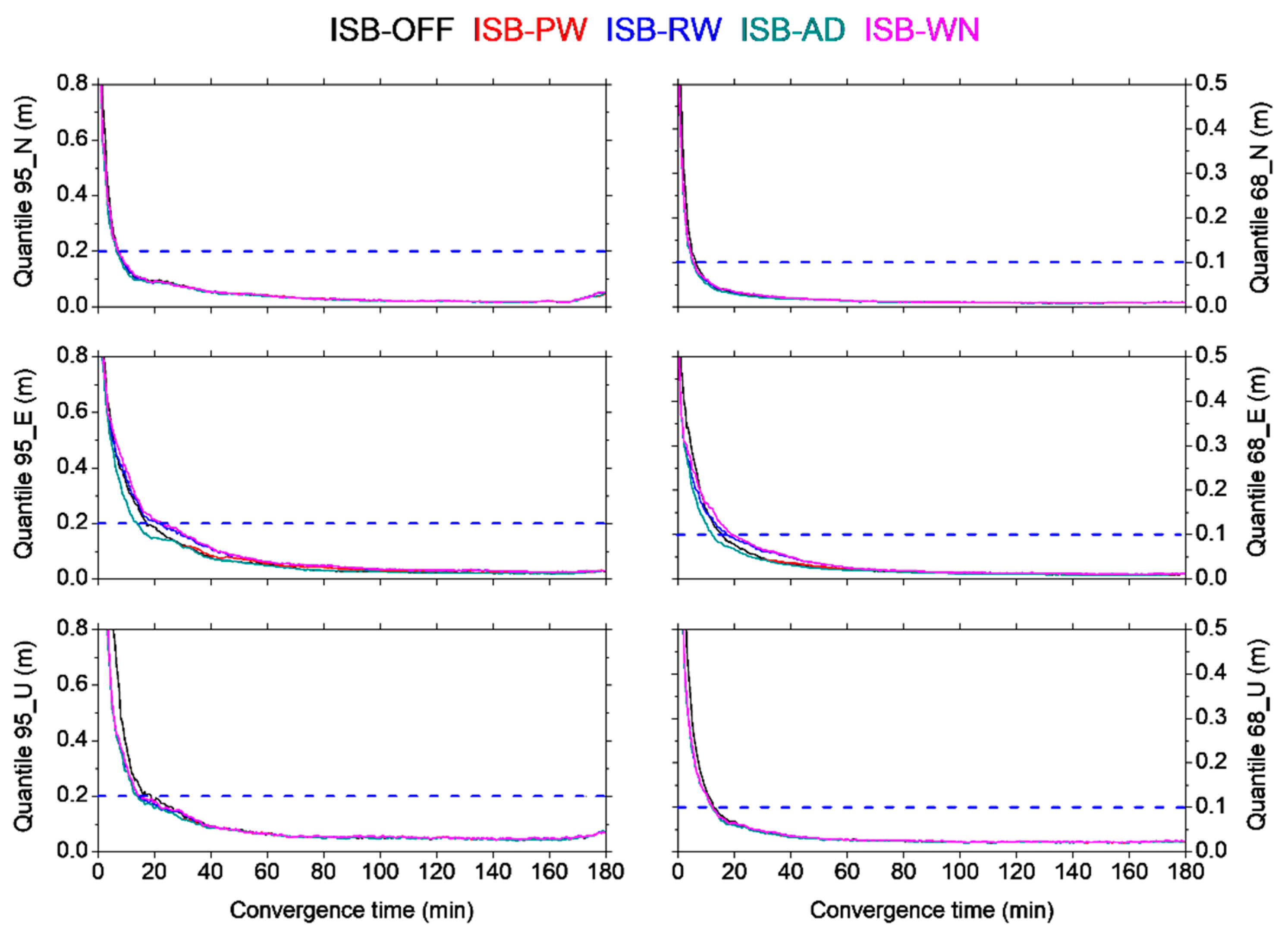
Figure 8 presents the errors in North (N), East (E), and UP (U) components of GPS/BDS combined static PPP in different schemes. Meanwhile, Table 4 shows the convergence time derived in the N, E, and U components, based on the statistics over all the tests.
From Figure 8 and Table 4, it can be noticed that PPP performance at some components in ISB-OFF, and ISB-AD schemes cannot converge in one 3-h processing-arc window. It also can be seen that using the GBM products, the convergence time of ISB-OFF is 8.5 min and 20.0 min in N, and U components at 95% quantile. It takes 7.5 min, 74.5 min and 16.0 min to converge into the 68% quantile in three components. As for the N component, the convergence time of four schemes with ISB (ISB-PW, ISB-RW, ISB-AD, and ISB-WN) is on average improved by 41.2% from 8.5 min to 5.0 min, and 41.7% from 7.5 min to 4.4 min at 95% and 68% quantile, respectively. That means after considering the ISB, the convergence rate speeds up, compared to ISB-OFF. The convergence time of ISB-PW at the U component is longer than ISB-OFF, this may be caused by the stochastic model of ISB-PW here being inconsistent with the model of ISB estimation applied by GFZ for precise product generation, which is not mentioned in any reference, but we have confirmed with the colleagues responsible for the matter in GFZ. From the results, this inconsistency will slow down the ISB convergence rate, and PPP performance time will be increased. This finding corresponds with the results in Figure 6. At E component, ISB-PW performs faster than ISB-OFF. It also can be seen that ISB-RW and ISB-WN have similar results and perform best among the proposed schemes. ISB-PW performs better than ISB-AD, and at the end of the 3-h period, its accuracy can reach closer to ISB-RW, and ISB-WN. It is quite incredible that compared with ISB-OFF, ISB-AD has a poorer result. In other words, GPS/BDS combined PPP considering the ISB with GBM products performs worse than neglecting the ISB, which is largely due to the inconsistency of ISB stochastic model applied in PPP processing on the user side and the precise products generation in GFZ. Therefore, we recommend PPP users adopt the same stochastic model of ISB estimation as the analysis center.
Figure 9 indicates the errors in N, E, and U components of kinematic PPP with different schemes, and Table 4 also shows the convergence time of kinematic PPP at the 95% and 68% quantile in three different components. It can be seen that the convergence times of all schemes in kinematic mode are longer than the static mode, because of different coordinate estimation strategies. However, similar to the static PPP, both at 95% and 68% quantile, ISB-AD performs worst in the convergence performance, while ISB-RW and ISB-WN perform best. PPP performance cannot be converged in E and U components for ISB-OFF, and ISB-AD at 95% quantile. For the 68% quantile, there are no convergence time values in E component. Compared with ISB-PW, the convergence time of ISB-RW at 95% quantile can be improved by 71.7% from 72.5 min to 20.5 min in E component, and 47.8% from 34.5 min to 18.0 min in U component, respectively. As for the 68% quantile, the improvement can reach 74.8% from 63.5 min to 16.0 min in E component, and 45.1% from 25.5 min to 14.0 min. ISB-WN has a similar convergence time as ISB-RW. It can also be noted that the convergence time in U component is less than that in E component in ISB-PW, ISB-RW, and ISB-WN. The first reason may be the phase ambiguities are more correlative with the E component than U component. Thus, in some cases, the convergence time of E component will be enlarged because of their correlation with phase ambiguities [35]. The second reason may be caused by the GPS and BDS satellites with north-south ground tracking in the earth-fixed reference frame [27].
GPS/BDS combined positioning accuracy in static and kinematic modes for five different schemes is listed in Table 5. In static PPP, we make the statistics using the results in the last epoch. As for the kinematic mode, since PPP performance cannot converge in some schemes, we make statistics with the same processing period, here using two hours later for each test. We can see, from the table, ISB-RW and ISB-WN have a similar processing accuracy, and perform best, while ISB-AD performs worst. Compared with ISB-AD, in static PPP at 95% quantile, the accuracy of ISB-RW and ISB-WN are improved by 90% from 12.0 cm to 1.2 cm, 95.6% from 36.3 cm to 1.6 cm, and 91.8% from 34.3 cm to 2.8 cm in N, E, and U components, respectively. At 68% quantile, the remarkable improvement can also be achieved with 80.6%, 96.3%, and 89.8% in three components. For kinematic mode at 95% quantile, the accuracy improvements are 89.5% from 19.1 cm to 2.0 cm, 94.1% from 50.6 cm to 3.0 cm, and 86.8% from 43.8 cm to 5.8 cm in N, E, and U components, respectively, while at 68% quantile, 89.9%, 94.8%, and 86.9% accuracy increment in three components can be acquired. Compared to ISB-OFF, schemes with the ISB parameter (i.e., ISB-PW, ISB-RW, and ISB-WN) can get an obvious accuracy improvement, which indicates the importance of considering ISB. Therefore, we conclude that from the validation of convergence time and performance accuracy using the GBM precise products, it is necessary to introduce the ISB parameter, and estimate it as a random-walk processing, or white noise, if you want to get a higher processing precision in a short time period (e.g., 3 h in this study). The scheme of ISB estimated as an arc-dependent constant (ISB-AD) is not recommended, because of its longest convergence time and worst positioning accuracy.
4.3.2. The Case with WUM Precise Products
The analysis of the convergence time and positioning accuracy in GPS/BDS combined kinematic PPP using WUM precise products is shown in Figure 10. Meanwhile, Table 6 presents the statistics of convergence time and positioning accuracy. The ISB stochastic model applied in AC Wuhan University is considered it as an arc-dependent constant [14]. From the figure and the table, we can see that different from the tests with the GBM products, the performance using the WUM products have similar accuracy level whether considering the ISB parameter or not. The possible reason is that ISB estimation strategy used in WUM products is the same as the ambiguity processing strategy, and both are estimated as a constant each arc window. Thus, the ISB is highly correlative with the ambiguity; in this case, if the ISB is not introduced, the impact of its error will be absorbed by ambiguity. This finding corresponds with the statements from Figure 7. For the convergence time, in N component the improvements are small (6.7% from 7.5 min to 7.0 min) at the 95% quantile, and at 68% quantile, it is on average 19.2%, from 6.5 min to 5.25 min. For the E component, the schemes ISB-PW and ISB-AD perform better than ISB-OFF, and ISB-RW is worse than ISB-OFF, while ISB-WN performs worst. Compared with ISB-WN, the convergence time of ISB-PW and ISB-AD can be improved by 40.4% from 23.5 min to 14.0 min, and 34.2% from 19.0 min to 12.5 min at 95% quantile and 68% quantile, respectively. Similar to N component, the improvements of convergence time in U component considering ISB are low, which can on average reach 16.2%, and 5.8% at 95% quantile, and 68% quantile, respectively.
From these two cases with GBM and WUM precise products, we can conclude that GPS/BDS combined PPP processing with orbit and clock products from different ACs can get a completely different result, because during the generations of multi-GNSS orbit and satellite clock products, different ISB resolution strategies (stochastic model) are applied in different ACs, and if the users use the same ISB strategies as the ACs (GBM and WUM) during the PPP performance, a better result can be obtained. So, based on the tests in this study, we recommend users consider the ISB parameter as random-walk processing, or white noise if the GBM products are used; however, when the WUM products are applied, it is better to consider the ISB as a piece-wise constant, or an arc-dependent constant.
4.4. Accuracy Improvement during the Convergence Period
During the convergence period, the accuracy of GPS/GLONASS combined PPP can be improved after considering the inter-frequency biases (IFB) [36]. So, similar analysis of accuracy improvement in GPS/BDS fusion PPP when considering ISB during the initialization phase is made in this study.
Table 7 and Table 8 show the statistics of the positioning accuracy during the convergence period. It can be seen from the tables that no matter which product is applied, if ISB is neglected, the accuracy in N, E, and U components is lower than the schemes with considering the ISB during 8 min and 16 min convergence period both at 95% and 68% quantiles. Therefore, we can conclude that considering ISB also has a great improvement on the PPP positioning accuracy during the convergence period. With GBM precise products, the average improved rate can be 40.1%, 35.4%, and 41.0% in N, E, and U components, respectively. In addition, for the WUM products, this rate can be 25.4%, 22.3%, and 33.4% in three components, respectively.
5. Conclusions
To study the effect of stochastic models for the ISB estimation and the importance of considering ISB, five different ISB processing strategies are proposed. From the comparison of pseudorange observation residuals between five strategies, it can be found that the ISB-OFF strategy has the largest residuals, and the other four schemes have much lower results. Compared to ISB-OFF, the RMS of pseudorange residuals in ISB-PW, ISB-RW, ISB-AD, and ISB-WN can reduce by 21.3 m (improvement rate is 95.9%) both in static mode and kinematic mode. That is to say, it is quite necessary to consider the effect of ISB parameter in multi-GNSS combined positioning.
As for the analyses on the convergence time and positioning accuracy, the cases with GBM and WUM precise products are carried out to reveal the potential impact on ISB caused by the different solution strategies in the analysis center. The result of the GBM case shows that ISB-RW and ISB-WN strategies have a similar processing accuracy, and perform best, while ISB-AD performs worst, even worse than the ISB-OFF, which is against the conclusion of pseudorange observation residuals results, the most probable reason being that the ISB stochastic model during GBM precise product generation is not set as an arc-dependent constant. The result of the WUM case is opposite; the schemes ISB-PW and ISB-AD perform best, and ISB-RW is worse than ISB-OFF, while ISB-WN performs worst. Based on the above findings, it can be concluded that the ISB processing strategies of GBM and WUM products are quite different. Thus, the recommendation of the ISB stochastic model selection can summarized as follows: it is better to consider the ISB parameter as random walk, or white noise if the GBM products are used; however, when the WUM products are applied, it is better to consider the ISB as a piece-wise constant, or an arc-dependent constant.
The test of accuracy improvement during the convergence period is performed as well. From the results, the conclusion can be drawn that just as after a converged period, considering ISB or not also has a strong impact on PPP positioning accuracy during the convergence period.
Author Contributions
N.J. and Y.X. conceived and designed the study, made formal analysis, wrote the original draft; T.X. made some data analysis and visualization, and interpreted the results; G.X. contributed to the project administration; H.S. polished the manuscript.
Funding
This study is supported by the Chinese Scholarship Council, Technical University of Berlin, German Research Centre for Geosciences Potsdam, and Institute of Space Sciences of Shandong University. This work is also funded by National Key Research Program of China “Collaborative Precision Positioning Project” (2016YFB0501900), State Key Laboratory of Geo-Information Engineering, China (SKLGIE2017-Z-2-2), National Natural Science Foundation of China (41874032, 41731069, 41574013, and 41574025).
Acknowledgments
The authors would like to thank the MGEX network for providing open access multi-GNSS observations.
Conflicts of Interest
The authors declare no conflict of interest.
References
- Aboul-Enein, Y.H. The Precision Revolution: GPS and the Future of Aerial Warfare. Tech. Cult. 2003, 45, 883–884. [Google Scholar]
- Revnivykh, S. GLONASS Status and Progress. In Proceedings of the ION GNSS 2010, Portland, OR, USA, 22 September 2010; pp. 609–633. [Google Scholar]
- Falcone, M. GALILEO System Status. In Proceedings of the ION GNSS 2016, Portland, OR, USA, 12–16 September 2016; pp. 2410–2430. [Google Scholar]
- Yang, Y. Progress, Contribution and Challenges of Compass/Beidou Satellite Navigation System. Acta Geod. Cartogr. Sin. 2010, 39, 1–6. [Google Scholar]
- Yang, Y.; Li, J.; Wang, A.; Xu, J.; He, H.; Guo, H.; Shen, J.; Dai, X. Preliminary assessment of the navigation and positioning performance of BeiDou regional navigation satellite system. Sci. China Earth Sci. 2014, 57, 144–152. [Google Scholar] [CrossRef]
- Montenbruck, O.; Steigenberger, P.; Khachikyan, R.; Weber, G.; Langley, R.B.; Mervart, L.; Hugentobler, U. IGS-MGEX: Preparing the ground for multi-constellation GNSS science. In Proceedings of the 4th International Colloquium on Scientific and Fundamental Aspects of the Galileo System, Prague, Czech Republic, 4–6 December 2013. [Google Scholar]
- Torre, A.D.; Caporali, A. An analysis of intersystem biases for multi-GNSS positioning. GPS Solut. 2015, 19, 297–307. [Google Scholar] [CrossRef]
- Montenbruck, O.; Hauschild, A.; Hessels, U. Characterization of GPS/GIOVE sensor stations in the CONGO network. GPS Solut. 2011, 15, 193–205. [Google Scholar] [CrossRef]
- Jiang, N.; Xu, Y.; Xu, T.; Xu, G.; Sun, Z.; Schuh, H. GPS/BDS short-term ISB modelling and prediction. GPS Solut. 2017, 21, 163–175. [Google Scholar] [CrossRef]
- Chen, J.; Wang, J.; Zhang, Y.; Yang, S.; Chen, Q.; Gong, X. Modeling and Assessment of GPS/BDS Combined Precise Point Positioning. Sensors 2016, 16, 1151. [Google Scholar] [CrossRef]
- Li, X.; Zhang, X.; Ren, X.; Fritsche, M.; Wickert, J.; Schuh, H. Precise positioning with current multi-constellation Global Navigation Satellite Systems: GPS, GLONASS, Galileo and BeiDou. Sci. Rep. 2015, 5, 8328. [Google Scholar] [CrossRef] [Green Version]
- Paziewski, J.; Wielgosz, P. Assessment of GPS + Galileo and multi-frequency Galileo single-epoch precise positioning with network corrections. GPS Solut. 2014, 18, 571–579. [Google Scholar] [CrossRef]
- Li, X.; Zus, F.; Lu, C.; Ning, T.; Dick, G.; Ge, M.; Wickert, J.; Schuh, H. Retrieving high-resolution tropospheric gradients from multiconstellation GNSS observations. Geophys. Res. Lett. 2015, 42, 4173–4181. [Google Scholar] [CrossRef]
- Guo, J.; Xu, X.; Zhao, Q.; Liu, J. Precise orbit determination for quad-constellation satellites at Wuhan University: Strategy, result validation, and comparison. J. Geodesy 2016, 90, 143–159. [Google Scholar] [CrossRef]
- Lou, Y.; Zheng, F.; Gu, S.; Wang, C.; Guo, H.; Feng, Y. Multi-GNSS precise point positioning with raw single-frequency and dual-frequency measurement models. GPS Solut. 2016, 20, 849–862. [Google Scholar] [CrossRef]
- Geng, J.; Li, X.; Zhao, Q.; Li, G. Inter-system PPP ambiguity resolution between GPS and BeiDou for rapid initialization. J. Geodesy 2019, 93, 383–398. [Google Scholar] [CrossRef]
- Geng, J.; Guo, J.; Chang, H.; Li, X. Toward global instantaneous decimeter-level positioning using tightly coupled multi-constellation and multi-frequency GNSS. J. Geodesy 2018. [Google Scholar] [CrossRef]
- Gioia, C.; Borio, D. A statistical characterization of the Galileo-to-GPS inter-system bias. J. Geodesy 2016, 60, 1279–1291. [Google Scholar] [CrossRef]
- Dach, R.; Schaer, S.; Lutz, S.; Meindl, M.; Beutler, G. Combining the Observations from Different GNSS. Presented at the EUREF 2010 Symposium, Gävle, Sweden, 2–5 June 2010; Volume 12. [Google Scholar]
- Geng, J.; Meng, X.; Dodson, A.H.; Teferle, F.N. Integer ambiguity resolution in precise point positioning: Method comparison. J. Geodesy 2010, 84, 569–581. [Google Scholar] [CrossRef]
- Defraigne, P.; Bruyninx, C. On the link between GPS pseudorange noise and day-boundary discontinuities in geodetic time transfer solutions. GPS Solut. 2007, 11, 239–249. [Google Scholar] [CrossRef]
- Ge, M.; Gendt, G.; Rothacher, M.; Shi, C.; Liu, J. Resolution of GPS carrier-phase ambiguities in Precise Point Positioning (PPP) with daily observations. J. Geodesy 2008, 82, 389–399. [Google Scholar] [CrossRef]
- Xu, G.; Xu, Y. GPS: Theory, Algorithms Application; Springer Publishing Company: Berlin/Heidelberg, Germany, 2016. [Google Scholar]
- Koch, K.; Yang, Y. Robust Kalman filter for rank deficient observation models. J. Geodesy 1998, 72, 436–441. [Google Scholar] [CrossRef]
- Yang, Y. Adaptively robust kalman filters with applications in navigation. In Sciences Geodesy-I; Springer: Berlin/Heidelberg, Germany, 2010; pp. 49–82. [Google Scholar]
- Hatch, R. The synergism of GPS code and carrier measurements. In Proceedings of the International Geodetic Symposium on Satellite Doppler Positioning; Physical Science Laboratory of the New Mexico State University: Las Cruces, NM, USA, 1983; pp. 1213–1231. [Google Scholar]
- Melbourne, W. The case for ranging in GPS-based geodetic systems. In Proceedings of the First International Symposium on Precise Positioning with the Global Positioning System, Rockville, MD, USA, 15–19 April 1985; pp. 373–386. [Google Scholar]
- Wubbena, G. Software developments for geodetic positioning with GPS using TI 4100 code and carrier measurements. In Proceedings of the 1st International Symposium on Precise Positioning with the Global Positioning System, Rockville, MD, USA, 15–19 April 1985; pp. 403–412. [Google Scholar]
- Böhm, J.; Niell, A.; Tregoning, P.; Schuh, H. Global Mapping Function (GMF): A new empirical mapping function based on numerical weather model data. Geophys. Res. Lett. 2006, 33. [Google Scholar] [CrossRef] [Green Version]
- Wu, J.; Wu, S.; Hajj, G.; Bertiger, W.; Lichten, S. Effects of antenna orientation on GPS carrier phase. Astrodynamics 1992, 1, 1647–1660. [Google Scholar]
- Petit, G.; Luzum, B. IERS Conventions. In Proceedings of IERS Technical Note 36; Verlag des Bundesamts für Kartographie und Geodäsie: Frankfurt, Germany, 2010; Available online: https://www.iers.org/SharedDocs/Publikationen/EN/IERS/Publications/tn/TechnNote36/tn36.pdf;jsessionid=75EE4C0EE29A43CF4E0A45B6AA441D1A.live2?__blob=publicationFile&v=1 (accessed on 25 April 2019).
- de Oliveira, P.S., Jr.; Morel, L.; Fund, F.; Legros, R.; Monico, J.F.G.; Durand, S.; Durand, F. Modeling tropospheric wet delays with dense and sparse network configurations for PPP-RTK. GPS Solut. 2017, 21, 237–250. [Google Scholar]
- Bree, R.J.P.V.; Tiberius, C.C.J.M. Real-time single-frequency precise point positioning: Accuracy assessment. GPS Solut. 2012, 16, 259–266. [Google Scholar] [CrossRef]
- Zhou, F.; Dong, D.; Ge, M.; Li, P.; Wickert, J.; Schuh, H. Simultaneous estimation of GLONASS pseudorange inter-frequency biases in precise point positioning using undifferenced and uncombined observations. GPS Solut. 2018, 22, 19. [Google Scholar] [CrossRef]
- Blewitt, G. Carrier phase ambiguity resolution for the Global Positioning System applied to geodetic baselines up to 2000 km. J. Geophys. Res. Solid Earth 1989, 94, 10187–10203. [Google Scholar] [CrossRef]
- Shi, C.; Yi, W.; Song, W.; Lou, Y.; Yao, Y.; Zhang, R. GLONASS pseudorange inter-channel biases and their effects on combined GPS/GLONASS precise point positioning. GPS Solut. 2013, 17, 439–451. [Google Scholar]
Figure 1.
Distribution of the selected stations.

Figure 2.
Ionospheric-free pseudorange observation residuals of GPS and BDS systems at STR1 station as an example on DOY 251, 2017, here is the results of the first 3h period with static PPP mode, left column is the GPS system, the right one denotes the BDS system, from top to bottom represents different schemes.

Figure 3.
Ionospheric-free pseudorange observation residuals of GPS and BDS systems at STR1 station as an example on DOY 251, 2017, it is the results for the first 3h period with kinematic PPP mode.
Figure 3.
Ionospheric-free pseudorange observation residuals of GPS and BDS systems at STR1 station as an example on DOY 251, 2017, it is the results for the first 3h period with kinematic PPP mode.

Figure 4.
Ionospheric-free carrier-phase observation residuals for GPS and BDS satellites in STR1 station, the result in the first 3h period on DOY 251, 2017 with static PPP mode is taken as an example, left panels are the results for GPS system, the right ones denote the results of BDS system, from top to bottom represents different schemes.

Figure 5.
Ionospheric-free carrier-phase observation residuals in the first 3h period of DOY 251, 2017 for the kinematic PPP mode, left panels show the results for GPS system, the right ones are the results of BDS system.
Figure 5.
Ionospheric-free carrier-phase observation residuals in the first 3h period of DOY 251, 2017 for the kinematic PPP mode, left panels show the results for GPS system, the right ones are the results of BDS system.

Figure 6.
The estimated ISBs derived from the four different schemes with considering ISB using the GBM products. Different ISBs are shown in different colors. The top subfigure displays the results for the static mode, while the bottom on is the results for the kinematic mode.
Figure 6.
The estimated ISBs derived from the four different schemes with considering ISB using the GBM products. Different ISBs are shown in different colors. The top subfigure displays the results for the static mode, while the bottom on is the results for the kinematic mode.

Figure 7.
The estimated ISBs using the WUM products in the kinematic mode. Different ISBs derived from the different schemes with considering ISB are shown in different colors.
Figure 7.
The estimated ISBs using the WUM products in the kinematic mode. Different ISBs derived from the different schemes with considering ISB are shown in different colors.

Figure 8.
GPS/BDS combined static PPP convergence performance in five different schemes with GBM precise products, each scheme uses a different color, left side is the errors of 95% quantile, while the right side is the errors of 68% quantile.
Figure 8.
GPS/BDS combined static PPP convergence performance in five different schemes with GBM precise products, each scheme uses a different color, left side is the errors of 95% quantile, while the right side is the errors of 68% quantile.

Figure 9.
GPS/BDS combined kinematic PPP convergence performance with five different schemes.

Figure 10.
GPS/BDS combined kinematic PPP convergence performance in five different schemes using WUM precise products.
Figure 10.
GPS/BDS combined kinematic PPP convergence performance in five different schemes using WUM precise products.


Table 1.
Models and strategies for data processing.
| Item | Models/Strategies |
|---|---|
| Data | GPS + BDS, 8 stations |
| Processing-arc-window | 3 h, 8 stations in one-week period have totally 448 tests |
| Signal selection | GPS:L1 and L2; BDS:B1 and B2 |
| Estimator | Kalman filter |
| Elevation cut off | 7° |
| Interval rate | 30 s |
| Satellite orbit and clock | Fixed to MGEX (GBM or WUM) products |
| Tropospheric delay | Saastamoinen model corrected for the dry component; estimate the residual wet component with random-walk processing |
| Mapping function | Global Mapping Function (GMF) |
| Ionospheric delay | First-order effect eliminated by ionospheric-free linear combination |
| Receiver phase center | PCO and PCV for GPS from igs14.atx are used; Corrections of BDS is applied the same with GPS |
| Satellite phase center | PCO and PCV are used with igs14.atx |
| ISB | Schemes ISB-OFF, ISB-PW, ISB-RW, ISB-AD, ISB-WN |
| Phase ambiguities | Estimated as a constant for each arc |
Table 2.
The description of GPS/BDS ISB estimating schemes.
| Schemes | Descriptions |
|---|---|
| ISB-OFF | Neglecting inter-system bias |
| ISB-PW | Estimating the ISB as piece-wise constant |
| ISB-RW | Estimating the ISB as a random-walk processing |
| ISB-AD | Estimating the ISB as a processing-arc-dependent constant |
| ISB-WN | Estimating the ISB as white noise |
Table 3.
Details of 8 selected stations location and receiver types.
| Station ID | Location | Receiver Type | ||
|---|---|---|---|---|
| Latitude (°) | Longitude (°) | Height (m) | ||
| CUT0 | −32.0039 | 115.8948 | 24.000 | TRIMBLE NETR9 |
| KARR | −20.9814 | 117.0972 | 109.247 | TRIMBLE NETR9 |
| MRO1 | −26.6966 | 116.6375 | 354.069 | TRIMBLE NETR9 |
| PERT | −31.8019 | 115.8852 | 12.920 | TRIMBLE NETR9 |
| MOBS | −37.8294 | 144.9753 | 40.578 | SEPT POLARX4TR |
| NNOR | −31.0487 | 116.1927 | 234.984 | SEPT POLARX4 |
| STR1 | −35.3155 | 149.0109 | 800.032 | SEPT POLARX5 |
| YAR2 | −29.0466 | 115.3470 | 241.291 | SEPT POLARX4TR |
Table 4.
Convergence times of GPS and BDS combined static and kinematic PPP in five different schemes (unit: min).
Table 4.
Convergence times of GPS and BDS combined static and kinematic PPP in five different schemes (unit: min).
| Static (95%) | Static (68%) | Kinematic (95%) | Kinematic (68%) | |||||||||
|---|---|---|---|---|---|---|---|---|---|---|---|---|
| N | E | U | N | E | U | N | E | U | N | E | U | |
| OFF | 8.5 | - | 20.0 | 7.5 | 74.5 | 16.0 | 14.5 | - | - | 11.5 | - | 25.0 |
| PW | 5.0 | 63.0 | 31.0 | 4.5 | 45.5 | 31.0 | 7.5 | 72.5 | 34.5 | 6.0 | 63.5 | 25.5 |
| RW | 5.0 | 13.0 | 13.5 | 4.0 | 11.5 | 12.0 | 7.0 | 20.5 | 18.0 | 5.5 | 16.0 | 14.0 |
| AD | 5.0 | - | - | 4.5 | - | - | 7.5 | - | - | 6.0 | - | 25.5 |
| WN | 5.0 | 13.5 | 14.0 | 4.5 | 11.5 | 12.0 | 7.5 | 19.5 | 17.5 | 5.5 | 17.5 | 13.5 |
Table 5.
Positioning accuracy of GPS/BDS combined static and kinematic PPP with five different schemes (unit: cm).
Table 5.
Positioning accuracy of GPS/BDS combined static and kinematic PPP with five different schemes (unit: cm).
| Static (95%) | Static (68%) | Kinematic (95%) | Kinematic (68%) | |||||||||
|---|---|---|---|---|---|---|---|---|---|---|---|---|
| N | E | U | N | E | U | N | E | U | N | E | U | |
| OFF | 9.5 | 31.9 | 23.6 | 1.3 | 9.3 | 4.3 | 14.6 | 34.6 | 31.8 | 4.6 | 12.7 | 10.7 |
| PW | 1.4 | 3.6 | 3.9 | 0.7 | 1.6 | 1.8 | 2.9 | 6.7 | 8.6 | 1.4 | 3.0 | 3.8 |
| RW | 1.2 | 1.6 | 2.7 | 0.7 | 0.7 | 1.3 | 2.0 | 3.0 | 5.8 | 0.8 | 1.3 | 2.6 |
| AD | 12.0 | 36.3 | 34.3 | 3.6 | 18.9 | 12.8 | 19.1 | 50.6 | 43.8 | 7.9 | 24.8 | 19.8 |
| WN | 1.2 | 1.6 | 2.8 | 0.7 | 0.7 | 1.3 | 2.0 | 3.0 | 5.8 | 0.8 | 1.3 | 2.6 |
Table 6.
Convergence time and positioning accuracy of GPS/BDS combined kinematic PPP with the WUM products in five different schemes.
Table 6.
Convergence time and positioning accuracy of GPS/BDS combined kinematic PPP with the WUM products in five different schemes.
| Convergence Time (95%)/min | Convergence Time (68%)/min | Accuracy (95%)/cm | Accuracy (68%)/cm | |||||||||
|---|---|---|---|---|---|---|---|---|---|---|---|---|
| N | E | U | N | E | U | N | E | U | N | E | U | |
| OFF | 7.5 | 17.5 | 17.0 | 6.5 | 15.5 | 13.0 | 4.9 | 6.1 | 7.6 | 2.0 | 2.7 | 3.2 |
| PW | 7.0 | 14.0 | 14.0 | 5.0 | 12.5 | 12.0 | 4.8 | 6.6 | 7.6 | 2.0 | 2.9 | 3.2 |
| RW | 7.0 | 21.0 | 14.5 | 5.5 | 17.5 | 12.5 | 5.0 | 7.0 | 7.8 | 2.1 | 3.3 | 3.3 |
| AD | 7.0 | 14.0 | 14.0 | 5.0 | 12.5 | 12.0 | 4.8 | 6.2 | 7.4 | 2.0 | 2.7 | 3.1 |
| WN | 7.0 | 23.5 | 14.5 | 5.5 | 19.0 | 12.5 | 5.2 | 6.8 | 8.0 | 2.2 | 3.3 | 3.3 |
Table 7.
Positioning accuracy of GPS/BDS combined kinematic PPP during the convergence period (8 min and 16 min) in five different schemes with GBM precise products (unit: cm).
Table 7.
Positioning accuracy of GPS/BDS combined kinematic PPP during the convergence period (8 min and 16 min) in five different schemes with GBM precise products (unit: cm).
| 8 min (95%) | 16 min (95%) | 8 min (68%) | 16 min (68%) | |||||||||
|---|---|---|---|---|---|---|---|---|---|---|---|---|
| N | E | U | N | E | U | N | E | U | N | E | U | |
| OFF | 71.4 | 78.4 | 191.8 | 76.1 | 94.7 | 178.7 | 49.3 | 57.9 | 106.1 | 35.6 | 45.5 | 76.4 |
| PW | 58.2 | 69.3 | 135.6 | 43.3 | 58.8 | 100.0 | 24.6 | 31.4 | 58.1 | 18.1 | 27.1 | 42.7 |
| RW | 58.7 | 71.2 | 135.9 | 42.9 | 53.1 | 99.0 | 24.3 | 30.6 | 57.4 | 17.6 | 23.7 | 41.5 |
| AD | 58.2 | 69.3 | 135.6 | 43.4 | 58.8 | 100.0 | 24.6 | 31.4 | 58.1 | 18.1 | 27.1 | 42.7 |
| WN | 60.5 | 69.9 | 137.1 | 43.8 | 54.3 | 99.2 | 24.6 | 31.1 | 57.5 | 17.8 | 24.3 | 41.5 |
Table 8.
Positioning accuracy of GPS/BDS combined kinematic PPP during the convergence period (8 min and 16 min) in five different schemes with WUM precise products (unit: cm).
Table 8.
Positioning accuracy of GPS/BDS combined kinematic PPP during the convergence period (8 min and 16 min) in five different schemes with WUM precise products (unit: cm).
| 8 min (95%) | 16 min (95%) | 8 min (68%) | 16 min (68%) | |||||||||
|---|---|---|---|---|---|---|---|---|---|---|---|---|
| N | E | U | N | E | U | N | E | U | N | E | U | |
| OFF | 104.8 | 122.8 | 247.2 | 51.3 | 59.7 | 137.7 | 32.1 | 38.7 | 82.0 | 23.0 | 29.1 | 58.6 |
| PW | 59.2 | 68.7 | 136.9 | 42.0 | 52.0 | 97.6 | 25.3 | 30.5 | 57.0 | 18.2 | 22.9 | 41.0 |
| RW | 59.3 | 68.2 | 136.8 | 42.5 | 55.5 | 98.0 | 25.4 | 31.4 | 57.0 | 18.4 | 24.3 | 41.1 |
| AD | 59.2 | 68.7 | 136.9 | 42.0 | 52.0 | 97.6 | 25.3 | 30.5 | 57.0 | 18.2 | 22.9 | 41.0 |
| WN | 59.6 | 73.4 | 137.0 | 43.2 | 57.6 | 98.8 | 25.7 | 32.5 | 57.6 | 18.6 | 25.6 | 41.5 |
© 2019 by the authors. Licensee MDPI, Basel, Switzerland. This article is an open access article distributed under the terms and conditions of the Creative Commons Attribution (CC BY) license (http://creativecommons.org/licenses/by/4.0/).
Share and Cite
MDPI and ACS Style
Jiang, N.; Xu, T.; Xu, Y.; Xu, G.; Schuh, H. Assessment of Different Stochastic Models for Inter-System Bias between GPS and BDS. Remote Sens. 2019, 11, 989. https://0-doi-org.brum.beds.ac.uk/10.3390/rs11080989
AMA Style
Jiang N, Xu T, Xu Y, Xu G, Schuh H. Assessment of Different Stochastic Models for Inter-System Bias between GPS and BDS. Remote Sensing. 2019; 11(8):989. https://0-doi-org.brum.beds.ac.uk/10.3390/rs11080989
Chicago/Turabian StyleJiang, Nan, Tianhe Xu, Yan Xu, Guochang Xu, and Harald Schuh. 2019. "Assessment of Different Stochastic Models for Inter-System Bias between GPS and BDS" Remote Sensing 11, no. 8: 989. https://0-doi-org.brum.beds.ac.uk/10.3390/rs11080989
Note that from the first issue of 2016, this journal uses article numbers instead of page numbers. See further details here.