Increasing Precision for French Forest Inventory Estimates using the k-NN Technique with Optical and Photogrammetric Data and Model-Assisted Estimators

Abstract

Multisource forest inventory methods were developed to improve the precision of national forest inventory estimates. These methods rely on the combination of inventory data and auxiliary information correlated with forest attributes of interest. As these methods have been predominantly tested over coniferous forests, the present study used this approach for heterogeneous and complex deciduous forests in the center of France. The auxiliary data considered included a forest type map, Landsat 8 spectral bands and derived vegetation indexes, and 3D variables derived from photogrammetric canopy height models. On a subset area, changes in canopy height estimated from two successive photogrammetric models were also used. A model-assisted inference framework, using a k nearest-neighbors approach, was used to predict 11 field inventory variables simultaneously. The results showed that among the auxiliary variables tested, 3D metrics improved the precision of dendrometric estimates more than other auxiliary variables. Relative efficiencies (RE) varying from 2.15 for volume to 1.04 for stand density were obtained using all auxiliary variables. Canopy height changes also increased RE from 3% to 26%. Our results confirmed the importance of 3D metrics as auxiliary variables and demonstrated the value of canopy change variables for increasing the precision of estimates of forest structural attributes such as density and quadratic mean diameter.

1. Introduction

French forests, as with their European counterparts, undergo rapid changes, mainly due to the abandonment of agricultural lands [1]. In France, forests are defined as land areas of at least 0.5 ha with a minimum average width of 20 m, and a canopy cover of trees capable of reaching a height of 5 m in situ of more than 10% [2]. French forest area expanded by around 100,000 ha per year during the last century, and the phenomenon is showing no signs of diminishing. Similarly, forest-growing stock experienced the same trend with a time lag, and even doubled during the last 50 years [3]. As the French National Forest Inventory (NFI) is continuous, with a new sample generated each year, such an expansion is handled with a sample size adapted yearly to these new conditions [4]. Nevertheless, a large proportion of these new resources are located in areas where the intensity of forest management practices has been historically limited. These new resources have different properties compared to ancient forests [3], and remain largely unknown by local stakeholders. Support for action by territorial decision-makers, forest industry, and local administrations, requires precise estimation of forest resources at larger spatial scales for establishing forest management strategies under sustainable development. As the number of NFI plots at those scales is usually limited, alternative solutions must be developed.

Multisource national forest inventory (MSNFI) methods have been applied (e.g., [5,6,7]) to improve the precision of forest resource estimates without increasing inventory costs or sampling intensities for smaller areas than normally possible using NFI field data alone [8]. MSNFI relies on the combination of field inventory data with wall-to-wall auxiliary variables derived from thematic maps and remotely sensed data. The objective of MSNFI methods is to infer population parameters [6,9]. Design-based estimators [10] are well adapted to NFI data because they rely on probability sampling designs as the basis for inference and are nearly design-unbiased [11,12,13,14]. A model-based approach is an alternative which assumes that the population under study is a random realization of a “super-population”, but is subject to bias [15] and requires the use of a correctly specified model form [16,17]. Each method has its advantages and drawbacks [11], and the appropriate inference approach should be selected according to the objectives of interest because the respective estimators are based on different underlying assumptions [18,19,20].

MSNFIs have been implemented using either parametric or non-parametric models [21,22,23,24], including co-kriging, universal kriging, Bayesian regression model, geographically weighted regression, and k nearest neighbors (k-NN) [8,25,26,27,28]. Among these methods k-NN approaches have gained popularity in MSNFIs because of their multivariate properties [24,29], allowing simultaneous prediction of multiple forest attributes with a single model, and the absence of assumptions regarding the distributions of both response and auxiliary variables. A strong argument for k-NN relies on its ease of use and the fact that predictions better preserve the covariances among the observed forest response variable observations [24]. Overall, the performance of k-NN relies on the number of neighbors, k, the distance metric, the weights used for individual neighbors, and the auxiliary variables to build the model [30,31]. The optimal value of k is a trade-off between accuracy and variance. Single nearest neighbor (k = 1) uses only a single sample plot value in the imputations [15,32,33], and avoids extrapolation beyond bounds of reality [34], but at the cost of a reduced prediction accuracy [35]. A greater k value (>3 to 10 or much greater) selected based on an optimization criterion (e.g., prediction error) using the leave-one-out technique generally improves predictive accuracy [20,36].

In terms of variables, the majority of MSNFIs rely on freely available medium (i.e., Landsat TM) or coarse (i.e., MODIS) resolution optical images [8,37] due to their availability over large territories and their frequent renewal [38]. However, the correlation between optical variables and major forest attributes such as volume or biomass may be weak due to signal saturation problems [39]. Haapanen and Tuominen [40] combined Landsat TM data with textural features extracted from aerial photographs and reported that the combination of variables from both data sources provided the greatest predictive accuracies. The development of three-dimensional remote sensing from both spaceborne and airborne platforms provides information related to canopy height and structure that is well-correlated with some of the major forest attributes measured in the field [19,31,41], and is expected to provide greater accuracies for forest attribute estimates [42]. Studies have been conducted using Airborne Laser Scanning (ALS) data [43,44], Digital Aerial Photography (DAP) [41,45,46], and even Interferometric Synthetic Aperture Radar (InSAR) [47]. Estimates obtained using auxiliary variables derived from image matching techniques were found to be in good agreement with estimates obtained using ALS-derived variables [48,49]. The availability and affordability of aerial photographs at frequent intervals make them a viable alternative for forest inventory applications for updating or retrospective analysis compared to ALS or InSAR data [45,50,51]. Furthermore, multi-temporal aerial photographs also facilitate estimation of growth increment or canopy change detection that may improve the precision of MSNFI estimates. Typically, studies have employed simple height-related metrics (e.g., mean height, percentiles, maximum height) for forest attribute estimation (e.g., [52]). Other studies focus on more complex descriptors of canopy structure and heterogeneity at the plot-level [53,54,55]. The proliferation of auxiliary information poses the issue of the curse of dimensionality [56] and the related noise introduced by variables unrelated to response attributes of interest. For k-NN, the value of k can then be large when the relationship between field attributes and auxiliary variables is weak, and the selection of nearest neighbors may become difficult [20].

According to [57], more than 35% of studies involving k-NN approaches focused on boreal coniferous forests, and most of the studies on temperate continental and temperate mountain forests were for the USA. Despite the multivariate capabilities of k-NN, many researchers focused on a single response variable [20,58,59]. In this context, the objective of this paper was to test the performance of MSNFI based on multivariate k-NN imputations for improving the precision of estimates beyond what could be obtained by NFI field data alone in a broadleaved-dominated forest, which is complex in terms of composition, structure, and fragmentation. The secondary objectives were: 1) to assess the influence of auxiliary data (Landsat images, 3D models from aerial images and forest type map) on the precision of the MSNFI estimates, and 2) to further evaluate the potential of diachronic 3D data from two successive aerial data coverages on the precision of MSNFI estimates. The performance of MSNFI was evaluated in a multivariate context with 11 forest attributes as response variables: growing stock volume, production volume, basal area, density, quadratic mean diameter, and the volume respectively of broadleaved, conifers, oak, Scots pine, other broadleaved, and other conifers.

2. Materials and Methods

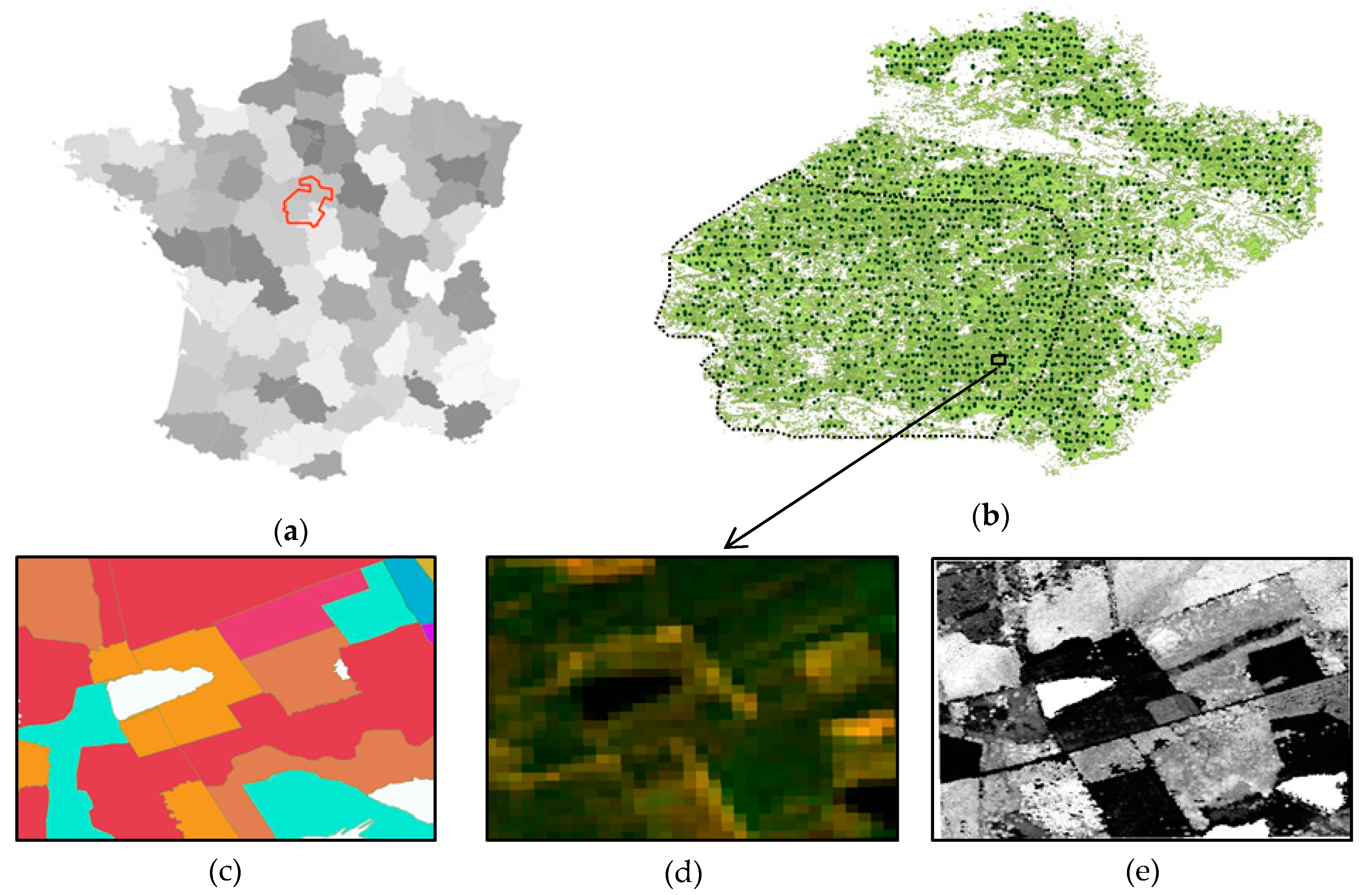
2.1. Study Site

The study site is located in Central France (48°6′ N to 48°5′ N and 1°50′ E to 1°30′ E) and covers the Sologne and Orléans forests, an area of 7335 km², of which 48% consists of forests (3600 km²) (Figure 1). The area is representative of western oak-dominated broadleaved French forests with respect to landscape heterogeneity, forest habitats, and diversity in forest management practices [60]. The area is influenced by a degraded oceanic climate and is marked by a greater temperature range compared with the littoral area. Mean annual temperature and precipitation are 10.9 °C and 731 mm, respectively. The slowly undulating relief ranges from 70 to 180 m elevations, and bears hydromorphic (58%), brown (23%), and podzolized (17%) soils made of sand and clay, and resulting from the erosion of the Massif Central. The forests are dominated by broadleaved (75.3%) mainly oaks (i.e., Quercus robur L. and Quercus petraea Mill.). Coniferous stands represent 15.5% of the forest area and are dominated by maritime (Pinus pinaster Ait.) and Scots pines (Pinus sylvestris L.). The remaining area of the forests is covered by mixed stands consisting mostly of oak and Scots pine. The forests are characterized by different management strategies related to forest ownership. While the southern part of the area is dominated by private forests (90%) with various intensities of management, the northern part is more intensely managed and includes the largest state forest of France, which covers around 34,600 ha.

2.2. National Forest Inventory Data

The French NFI is a continuous countrywide inventory [1,61]. The two-phase sampling plan is based on a permanent systematic 1-kilometer-square unit grid. The first-phase annual sample is drawn randomly for one-tenth of the grid (10 km²). For each 1-kilometer square grid cell one to four points may be drawn, thus constructing an annual sample of ~80,000 points. The first phase points are photo interpreted on 0.5 m resolution infrared aerial photographs for land cover and land use, and produce results for land cover. The second phase is a subsample of the first taken in different proportions. For forests, the standard second phase sample is obtained by taking one point out of two (~6500 points) that are visited in the field. Field observations are obtained from concentric plots of 6, 9, 15, and 25 m radius. The stand description in terms of land cover and use, as well as composition, structure, age, etc. is assessed for the 25 m plot. Trees are measured on the three smallest concentric plots, according to their circumference at a height of 1.3 m: trees in the 23.5–70.5 cm circumference range are measured on the 6 m radius plot, trees in the 70.5–117.5 cm circumference range are measured on the 9 m radius plots, and the trees with a circumference of at least 117.5 m are measured on the 15 m radius plot. Dendrometric measurements include species, diameter at 0.1 and 1.3 m, total height, as well as diameter increment during the last five years. Additional measurements including timber height, mid-diameter and mid-timber diameter are taken on a subsample of plots to fit volume models [1].

For the purpose of this research, data from 775 plots measured during the 5-year period 2010–2014 were used. This period has been selected to match the acquisition date of the remotely sensed data whose reference year was 2014. A total of 11 forest attributes were considered as response variables: growing stock volume, basal area, density, and quadratic mean diameter, production volume (estimated based on measurements of the last 5 growth rings), volumes of broadleaved, conifers, oak, Scots pine, other broadleaved and other conifers. Summary statistics for the plot variables are provided in

Table 1. Mean and variance of field plot attributes for the whole area and the subset area.

Response Variable	Main Area (N = 775)		Subset Area (N = 346)
	Mean	Variance	Mean	Variance
1: Total volume (m3/ha)	152.14	13.03	143.64	28.27
2: Stand basal area (m2/ha)	20.14	0.15	19.49	0.34
3: Stand density (n/ha)	686.19	402.37	687.23	952.03
4: Quadratic mean diameter (cm)	23.50	0.18	22.82	0.35
5: Production volume (m3/ha/yr)	5.45	0.016	5.41	0.04
6: Conifers volume (m3/ha)	46.06	10.13	50.22	28.40
7: Broadleaved volume (m3/ha)	106.08	11.09	93.41	18.88
8: Oak volume (m3/ha)	72.15	8.81	61.69	14.79
9: Other broadleaved volume (m3/ha)	33.93	4.07	31.72	7.48
10: Scots pine volume (m3/ha)	22.22	5.91	23.61	15.81
11: Other conifers volume (m3/ha)	23.85	5.58	26.62	16.24

. Two photogrammetric elevation models (2008 and 2014) are available for a subset (~44%) of the study area (N = 346 plots, Table 1), and were used to assess the effect of canopy height changes on the precision of estimates.

2.3. Auxiliary Data

Three sources of auxiliary data available at no cost were considered: a forest type (FT) map (BD Forêt^® v2) constructed by the French National Institute of Geographic and Forest Information (IGN), DAP models of the forest canopy surface, and Landsat images. All auxiliary variables were processed at a 30 m spatial resolution corresponding to the Landsat image pixel size and to the field plot area used for dendrometric measurements.

The FT map product BD Forêt^® is a vector layer constructed by photo-interpretation of near-infrared aerial photographs. The map includes a total of 32 classes and a minimum polygon size of 0.5 ha. The nomenclature includes a description of the vegetation type with the dominant species, according to tree cover classes. The map corresponding to the study region has been constructed using aerial images acquired in 2008. The forest contours were used to construct a forest mask. The mask was further intersected with the 30 m grid, and only the grid cells completely in the forest mask were considered for the analysis [10]. The FT map attributes were summarized for each grid cell and aggregated into three classes corresponding to pure broadleaved, pure conifers and mixed stands.

The DAP Digital Surface Models (DSM) were normalized using a co-occurring ALS Digital Terrain Model (DTM) to generate Canopy Height Models (CHM). ALS data were not considered as auxiliary data for describing the forest structure as their availability and cost prevent regular updates. The ALS data were acquired by IGN between January 17 and March 30, 2014, as part of the land survey with a point density of 2 pts.m⁻² and a flight line overlap of 50%. The point cloud was processed using the iterative TIN algorithm of the Terrascan software (Terrasolid, https://www.terrasolid.com, last consulted October 25, 2018), followed by visual inspection and manual correction whenever necessary. The algorithm was run using a terrain angle of 88°, iteration angle of 6°, and an iteration distance of 1.4 m. The point data were delivered by 1 km x 1 km tiles, and were buffered using a 30 m threshold. Ground classified points were used to construct a digital terrain model with a 1 m resolution using inverse distance weighted interpolation. The DAP DSMs were constructed using aerial images acquired in 2013 (eastern part of the area, from July 06 to 12), 2014 (western part of the area, from May 18 to July 16), and 2008 (western part of the area only). The 2013–2014 images were acquired using an IGN camera (sensor V28T, 14,650 x 10,700 pixels of 6.8 µm each) mounted with a Zeiss lens having a 125 mm focal length. The images were acquired at 6,400 m above ground level, leading to a 35 cm resolution at the ground level. The 2008 images were acquired on August 30 using a DMC camera (sensor of 13,824 x 7680 pixels of 9 µm each) and a Zeiss 90 mm focal length lens. The acquisition was done at an altitude of 5,500 m, leading to a 54 cm resolution at the ground level. For all flights, the image overlap was 60% along and 25% across tracks. The image orientation was done by IGN as part of the production process. The dense image matching was done using MicMac open source photogrammetric software [62]. MicMac is based on a multi-resolution-optimization approach and used a coarse to fine matching strategy based on image pyramids to improve the processing time and control the similarity of matches between levels. The dense matching was performed using a Per Images Matching approach (PIMs mode) in image geometry and rely on tie points generated using the ‘Scale-Invariant-Feature Transform’ (SIFT) detector [63]. The matching approach produces a depth map for each image pair. The depth maps are then merged together and converted into a dense point cloud. The resulting point clouds were converted into a 1 m DSM using the maximum height per pixels. Empty pixels were not interpolated. The DSM was further converted into a canopy height model (CHM) by subtracting the ALS DTM. Two categories of metrics were derived from the CHM to serve as auxiliary variables for each cell of the 30 m grid: distribution metrics above a height threshold fixed at 5 m to match with the definition of forest and structure metrics [53]. The distributional metrics included the percentiles 0 to 100 by steps of 10 (p0 to p100), as well as upper percentiles 95 and 99 (p95, p99), the mean (h_mean), standard deviation (h_std), variance (h_var), and the mean absolute deviation (h_mad) of heights. The structure metrics (

Table A1. Structure metrics derived from the photogrammetric canopy height model. N is the total number of pixels, P is a given pixel, and PS is the pixel size.

Metric Name	Acronym	Equation
Gap area	Ga	${\displaystyle \sum }_i^{n}CH{M}_{i<th}P{S}^2$
Mean inner canopy volume	Vi	$\frac{1}{n}{\displaystyle \sum }_i^{n}CH{M}_{i>th}P{S}^2$
Mean outer canopy volume	Vo	$\frac{1}{n}{\displaystyle \sum }_i^n(Pixe{l}_{CH{M}_{i>th}}\ast Max\left(CHM\right)\ast P{S}^2)-Vi$
Mean inner gap canopy volume	Vgi	$\frac{1}{n}{\displaystyle \sum }_i^{n}CH{M}_{i<th}P{S}^2$
Mean outer gap canopy volume	Vgo	$\frac{1}{n}{\displaystyle \sum }_i^n(P_{CH{M}_{i<th}}\ast Max\left(CHM\right)\ast P{S}^2)-Vgi$
Rumple area	Ra	${\displaystyle \sum }_{CHM>th}||\frac{\overrightarrow{P_{l,c}{P}_{l+1,c}}\wedge \overrightarrow{P_{l,c}{P}_{l,c+1)}}}{2}+\frac{\overrightarrow{P_{l+1,c+1}{P}_{l,c+1}}\wedge \overrightarrow{P_{l+1,c+1}+P_{l,c+1)}}}{2}\ast P{S}^2||/{\displaystyle \sum }_{CHM>th}P{S}^2$
No data	NA	${\displaystyle \sum }_i^n{P}_{CH{M}_{i=NA}}$

), included the gap area ratio (Ga), the mean inner canopy volume (Vi), the mean outer canopy volume (Vo), the mean inner canopy volume above a given threshold value (Th) fixed here at 5 m (Vci), the mean outer canopy volume above Th (Vco), defined as the complement of the canopy volume to the maximum height, the mean inner canopy volume within gaps (Vgi) and its outer complement (Vgo), the standard rumple area (Ra) [55], or the ones defined with respect to Vi (Ra1) and Vci (Ra2), as well as the number of empty pixels (NA). Over the subset area, various difference metrics were computed, including changes in gap area (dGa), in volume differences (e.g., dVi, dVo), mean, minimum and maximum heights (dh_mean, dp0, dp100), as well as in the upper percentiles (dp95, dp99).

Four Landsat 8 images acquired on September 8, 2014 were downloaded from the Theia platform (https://theia-landsat.cnes.fr) with the processing level 2A, including orthorectification, atmospheric correction and cloud detection [64]. The reflectance images were used to compute various indices (

Table A2. Landsat spectral indices. Acronyms B, R, NIR stand for blue, red, and near infra-red bands, respectively. SWIR stands for the shortwave Infrared bands. Ls and Lc are sol brightness correction factor and canopy background value, respectively. Ls is by default equal to 0.5 (Ls = 0 means NDVI = SAVI), and Lc is equal to 1.

Indice Name	Acronym	Equation
Simple Ratio	SR	NIR/R
Normalized Difference vegetation index	NDVI	(NIR − R)/(NIR + R)
Specific Leaf Area Vegetation Index	SLAVI	NIR/(R + SWIR1)
Soil Adjusted Vegetation Index	SAVI	((NIR − R)/(NIR + R+Ls)) * (1+Ls)
Modified Soil Adjusted Vegetation Index	MSAVI	(2 * NIR + 1 − $\sqrt{{\left(2\ast \mathrm{NIR}+1\right)}^2-8\ast \left(\mathrm{NIR}-\mathrm{R}\right))}$/2
Enhance Vegetation Index	EVI	2.5 * ((NIR − R)/(NIR + 6 * R − 7.5 * B + Lc))
Normalized Difference Moisture Index	NDMI	(R − NIR)/(R + NIR)
Normalized Difference Water Index	NDWI	(NIR − SWIR1)/(NIR + SWIR1)
Green NDVI	GNDVI	(NIR − G)/(NIR + G)
Brightness	Br	0.3029 B + 0.2786 G + 0.4733 R + 0.5599 NIR + 0.508 SWIR1 + 0.1872 SWIR2
Greenness	Gr	−0.2941 B − 0.243 G − 0.5424 R + 0.7276 NIR − 0.0713 SWIR1 − 0.1608 SWIR2
Wetness	We	0.1511 B + 0.1973 G + 0.3283 R + 0.3707 NIR − 0.7117 SWIR1 − 0.4559 SWIR2

): the simple ratio (SR), the normalized difference vegetation index (NDVI), the Specific Leaf Area Vegetation Index (SLAVI), the Soil Adjusted Vegetation Index (SAVI), the Modified Soil Adjusted Vegetation Index (MSAVI), the enhance vegetation index (EVI) the green NDVI (GNDVI), the Normalized Difference Moisture Index (NDMI), Normalized Difference Water Index (NDWI) [65,66], as well as brightness (Br), greenness (Gr), and wetness (We) derived from Tasseled Cap transformation [67]. In addition to computed spectral reflectance indices, we also included the seven reflectance bands of Landsat 8: Ultra Blue (UB), Blue (B), Green (G), Red (R), Near Infrared (NIR), Shortwave Infrared (SWIR) 1, and Shortwave Infrared (SWIR) 2. The Landsat metrics were assigned to the grid cells by intersecting the grid with the coordinate of the center of the Landsat pixels.

2.4. Optimization of the k-NN Model

MSNFI performance depends on: (1) the modeling framework, and (2) the correlation between the surveyed forest attributes and the auxiliary information.

As indicated above, a non-parametric multivariate k-NN approach was adopted to construct wall-to-wall predictions of forest attributes. The k-NN parameters include the number of neighbors (k), the distance metric used to search the variable space, and a weighting function to compute predictions [57]. In k-NN, the population units for which both response and auxiliary variables are available are termed the reference set and the units for which predictions of response variables are sought are termed the target set. The auxiliary variables are also termed feature variables and the space defined by them is termed the feature space.

Based on a literature survey [57,68] and preliminary results, two distance metrics were compared: Euclidean and Canonical Correlation Analysis (CCA) [69]. The Euclidean distance is computed in a normalized space of auxiliary variables. The CCA distance is defined by Equation (1):

$$\mathrm{d}=\sqrt{\mathsf{\Gamma }{\wedge }^2{\mathsf{\Gamma }}^{\mathrm{T}}}$$

(1)

where Γ is the matrix of canonical vectors corresponding to the X’s found by canonical correlation analysis between X and Y, ${\mathsf{\Gamma }}_{}^{\mathrm{T}}$ the transposed matrix, and $\wedge$ is the canonical correlation matrix.

Values of k in the range of 1 to 20 were tested to optimize model performance. The weight of the neighbors used to compute the imputed values for the continuous variables according to Equation (2):

w_j = 1/(1 + d_ij)

(2)

where d_ij is the distance between target pixel i and reference pixel j in the feature space.

k-NN models were generated using six different combinations of auxiliary variables: (1) Landsat variables alone, (2) Landsat variables and FT from the forest map, 3() 3D metrics from DAP CHMs, (4) 3D metrics from DAP CHMs with FT from the forest map, (5) Landsat variables and 3D metrics from DAP CHMs, and (6) all auxiliary variables. On the subset area, the introduction of change detection variables was also tested. Only two combinations of auxiliary variables were considered: all former auxiliary variables used alone, or with the change detection variables.

Note that preliminary analyses revealed estimation accuracy issues due to auxiliary variables having weak correlations with the response variables, which has also been reported in [30,31]. The problem was solved by filtering out auxiliary variables that have maximum correlation values less than 0.2 with the response variable considered. A total of four auxiliary variables were discarded from analysis, including three Landsat bands (UB, B, R), and one volume metric (Vco).

The performance of the k-NN models was evaluated using a leave-one-out cross-validation approach (LOOCV). Model accuracy was evaluated using the Root Mean Squared Difference (RMSD) between observed and imputed values [70]. For comparing imputation models across multiple response variables with different measurement units, RMSD value was standardized by dividing RMSD by the standard deviation of the observations of the response variable (i.e., Scaled RMSD = RMSD/Standard deviation of the response variable) [71]. Optimal k values were selected as those for which mean RMSD across multiple response variables did not differ more than 5% from the minimal mean RMSD value [20].

k-NN optimization was conducted using R open source software with the yaImpute package [71].

2.5. Statistical Inference

Using field data only, the design-based, simple expansion (Exp) estimators of the population mean and variance were defined by Equations (3) and (4).

$${\widehat{\mathsf{\mu }}}_{\mathrm{Exp}}^{}=\frac{1}{\mathrm{n}}{\displaystyle \sum }_{\mathrm{i}=1}^{\mathrm{n}}{\mathrm{y}}_{\mathrm{i}}$$

(3)

$$\mathrm{V}\widehat{\mathrm{a}}\mathrm{r}\left({\widehat{\mathsf{\mu }}}_{\mathrm{Exp}}^{}\right)=\frac{1}{\mathrm{n}\cdot \left(\mathrm{n}-1\right)}{\displaystyle \sum }_{\mathrm{i}=1}^{\mathrm{n}}{({\mathrm{y}}_{\mathrm{i}-}^{}{\widehat{\mathsf{\mu }}}_{\mathrm{Exp}}^{})}^2$$

(4)

where n is the number of sample plots, and ${\mathrm{y}}_{\mathrm{i}}$ is the observed value of plot i.

The inference of population parameters from the k-NN predictions across the study area was assessed using model-assisted generalized regression (GREG) estimators of means and variances [72]. Despite using the term regression in the label characterizing GREG estimators, multiple prediction techniques other than regression models, and particularly other than linear regression models, have been used with the GREG estimators [73,74,75]. The GREG estimator of the mean is the difference between the mean of the k-NN predictions across population units and the estimated bias, as shown in Equation (5):

$${\widehat{\mathsf{\mu }}}_{\mathrm{GREG}}^{}=\frac{1}{\mathrm{N}}{\displaystyle \sum }_{\mathrm{i}=1}^{\mathrm{N}}{\widehat{\mathrm{y}}}_{\mathrm{i}}-\frac{1}{\mathrm{n}}{\displaystyle \sum }_{\mathrm{i}=1}^{\mathrm{n}}{\mathsf{\epsilon }}_{\mathrm{i}}$$

(5)

where ${\mathsf{\epsilon }}_{\mathrm{i}}$ = (${\widehat{\mathrm{y}}}_{\mathrm{i}}-{\mathrm{y}}_{\mathrm{i}})$ is the difference between k-NN prediction and the observed response variable (estimate of bias), N is the number of population units or pixels, and n is the number of field sample plots. The associated variance estimator is computed using Equation (6):

$$\mathrm{V}\widehat{\mathrm{a}}\mathrm{r}\left({\widehat{\mathsf{\mu }}}_{\mathrm{GREG}}^{}\right)=\frac{1}{\mathrm{n}\cdot \left(\mathrm{n}-1\right)}·{\displaystyle \sum }_{\mathrm{i}=1}^{\mathrm{n}}{({\mathsf{\epsilon }}_{\mathrm{i}-}^{}\overline{\mathsf{\epsilon }})}_{}^2$$

(6)

where $\overline{\mathsf{\epsilon }}=\left(\frac{1}{\mathrm{n}}\right)·{{\displaystyle \sum }}_{\mathrm{i}=1}^{\mathrm{n}}{\mathsf{\epsilon }}_{\mathrm{i}}$.

The performance of k-NN was evaluated through a measure of relative efficiency (RE = $\mathrm{V}\widehat{\mathrm{a}}\mathrm{r}\left({\widehat{\mathsf{\mu }}}_{\mathrm{Exp}}^{}\right)$/$\mathrm{V}\widehat{\mathrm{a}}\mathrm{r}\left({\widehat{\mathsf{\mu }}}_{\mathrm{GREG}}^{}\right)$. RE provides an estimate of the gain in precision resulting from the use of the auxiliary information that is incorporated into the model-assisted estimators in comparison with pure field-based estimates. RE values greater than 1 indicate increased precision. The primary advantage of the GREG estimators is that they take advantage of the relationship between the probability based sample plot data and their corresponding predictions to reduce the variance of the estimated population mean [20] and thereby increase RE. For each combination of auxiliary variables: ${\widehat{\mathsf{\mu }}}_{\mathrm{GREG},}^{}\mathrm{V}\widehat{\mathrm{a}}\mathrm{r}\left({\widehat{\mathsf{\mu }}}_{\mathrm{GREG}}^{}\right)$, and RE were calculated for all 11 response variables.

2.6. External Validation

Internal models are recognized to underestimate variance [12,13]. To account for this issue, a complementary analysis was conducted. Both the main and subset areas were divided into three sub-areas having approximately the same number of field plots (i.e., 258 (~775/3) and 115 (~346/3) plots for the main and the subset areas, respectively). Each sub-area was used to build a k-NN model following the methods presented in Section 2.4 and Section 2.5. The models were then applied to the two other sub-areas as external models. The mean REs obtained with both approaches were compared to assess the underestimation associated with the internal model.

3. Results

3.1. k-NN Optimization

Table 2. Cross-validated Root Mean Squared Differences (RMSD) of the imputation, for the optimal k-NN models. Numbers in parenthesis are minimum and maximum values of the 11 forest attributes.

			Euclidean		CCA
Auxiliary Variable Combination	Domain	No. of Variables	k	RMSD	k	RMSD
Landsat	Main	15	6	1.00 (0.84;1.08)	6	0.99 (0.83;1.07)
Landsat & Forest types	Main	16	6	0.98 (0.73;1.09)	6	0.97 (0.71;1.07)
3D metrics	Main	24	6	0.91 (0.72;1.04)	6	0.91 (0.71;1.03)
3D metrics and Forest types	Main	25	5	0.85 (0.69;0.98)	5	0.84 (0.67,1.00)
3D metrics and Landsat	Main	39	8	0.86 (0.68;1.00)	5	0.86 (0.71;0.99)
All	Main	40	5	0.84 (0.67;1.00)	5	0.84 (0.64;0.97)
All	Subset	41	4	0.87 (0.66;1.02)	5	0.86 (0.66;1.01)
All and change	Subset	45	5	0.85 (0.65;1.00)	6	0.85 (0.64;1.01)

shows the mean RMSD values for the various combinations of auxiliary variables and distance metrics. The smaller the RMSD, the greater the similarity between the reference and the imputed observations. Using Euclidean distance, mean RMSD values ranged from 1.00 for the Landsat metrics alone to 0.84 for the overall metrics. The k values selected were relatively stable, ranging from 4 to 8. Interestingly, the combination of 3D metrics with the FT map performed well with a mean RMSD of 0.85, which was only 0.01 greater than for the combination having smaller RMSD with a 37.5% decrease in the number of auxiliary variables. By comparison, the combination of 3D metrics with Landsat metrics (39 variables) performed slightly less well with mean RMSD of 0.86, and a greater range of individual RMSD values. Slightly smaller RMSD values were obtained using CCA distance, with mean RMSD values ranging from 0.99 for the Landsat metrics alone to 0.84 with the full set of metrics. The optimal k value was also rather stable, ranging from 5 to 6. With both distance metrics, the introduction of canopy change auxiliary variables contributed to greater mean RMSD values. The improvement was more pronounced using the Euclidean distance metric, with a gain in mean RMSD of 0.02.

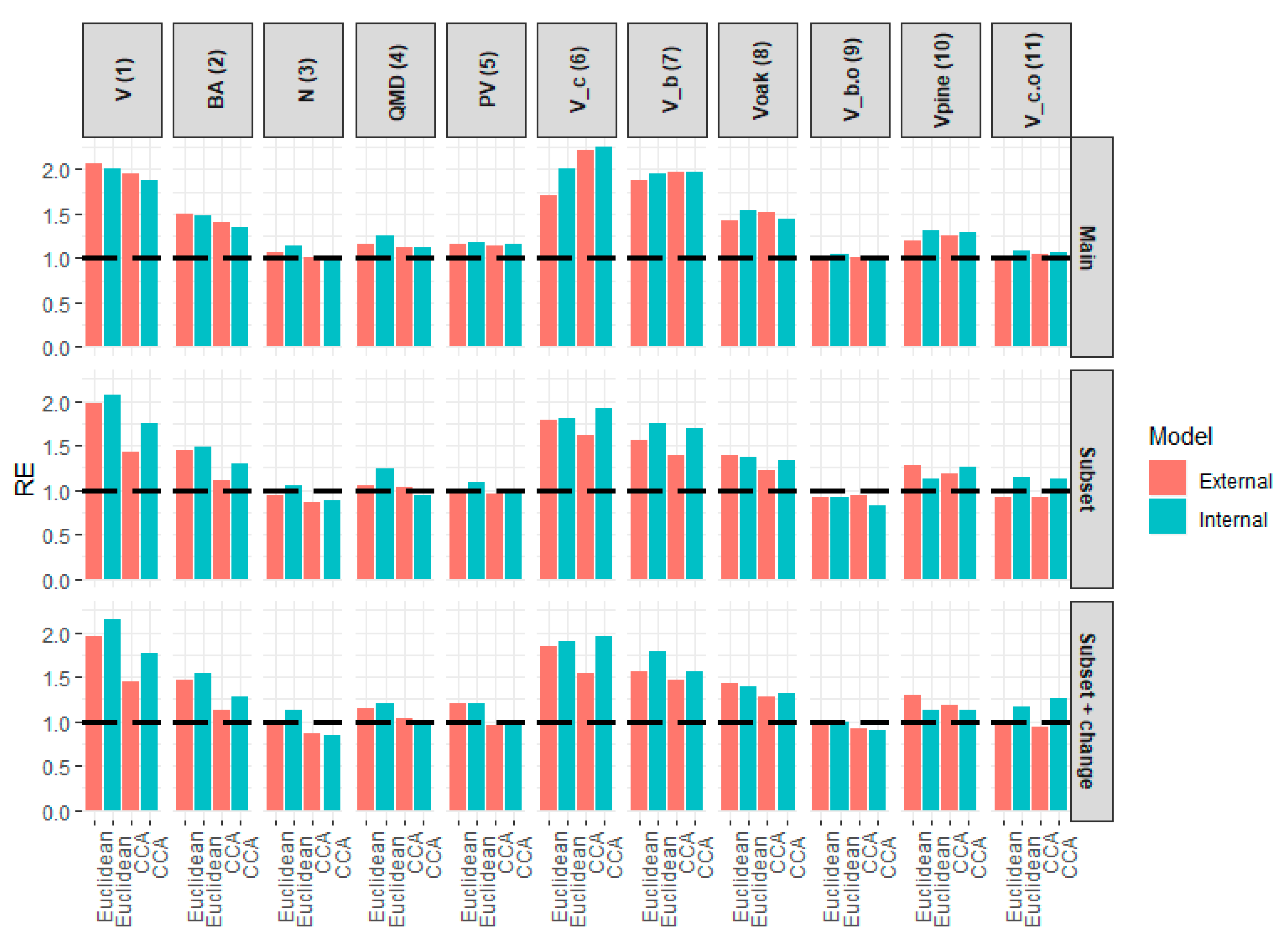
3.2. Statistical Inference

Table 3. Mean, standard error (SE), and relative efficiencies (RE) computed on the main area for the different combination of auxiliary variables using Euclidean distance. The greatest RE for each forest attributes appears in bold.

	Landsat			Landsat and Forest Types			3D Metrics
Forest Attributes 1	Mean	SE	RE	Mean	SE	RE	Mean	SE	RE
1	155.02	3.63	0.99	154.82	3.59	1.01	153.83	2.62	1.90
2	20.47	0.13	0.98	20.42	0.39	1.00	20.10	0.33	1.39
3	692.67	21.27	0.89	690.32	21.48	0.87	686.65	18.27	1.21
4	23.55	0.46	0.85	23.55	0.46	0.84	23.59	0.38	1.23
5	5.57	0.13	0.96	5.57	0.13	0.98	5.45	0.12	1.09
6	48.92	2.68	1.41	49.61	2.35	1.83	45.74	3.13	1.04
7	106.09	3.15	1.12	105.22	3.07	1.18	108.09	2.70	1.52
8	72.04	2.84	1.09	71.07	2.83	1.10	72.65	2.55	1.35
9	34.06	2.14	0.89	34.15	2.13	0.90	35.43	2.04	0.97
10	23.52	2.39	1.04	25.08	2.27	1.14	21.84	2.49	0.95
11	25.40	2.38	0.98	24.52	2.33	1.03	24.21	2.46	0.93
	3D Metrics and Forest Types			Landsat and 3D Metrics			All
Forest Attributes 1	Mean	SE	RE	Mean	SE	RE	Mean	SE	RE
1	155.28	2.55	2.00	153.60	2.48	2.12	153.24	2.44	2.18
2	20.33	0.32	1.43	20.00	0.31	1.54	19.98	0.31	1.56
3	691.73	18.37	1.19	673.84	19.07	1.11	678.00	19.17	1.10
4	23.54	0.39	1.20	23.64	0.38	1.22	23.48	0.38	1.23
5	5.49	0.12	1.16	5.45	0.12	1.18	5.47	0.12	1.19
6	47.66	2.19	2.10	48.69	2.44	1.70	47.91	2.18	2.13
7	107.62	2.31	2.07	104.91	2.39	1.93	105.33	2.29	2.11
8	72.12	2.41	1.52	72.20	2.33	1.63	72.29	2.28	1.69
9	35.50	1.99	1.03	32.71	2.02	0.99	33.05	2.02	1.00
10	22.72	2.15	1.28	24.40	2.27	1.14	23.68	2.15	1.28
11	24.94	2.32	1.04	24.28	2.36	1.01	24.23	2.27	1.08

¹: forest attributes: 1: total volume (m³/ha); 2: stand basal area (m²/ha); 3: stand density (stem/ha); 4: quadratic mean diameter (cm); 5: production volume (m³/ha/yr), 6: conifers volume (m³/ha); 7: broadleaved volume (m³/ha); 8: Oak volume (m³/ha), 9: other broadleaved volume (m³/ha); 10: Scots pine volume (m³/ha); 11: other conifers volume (m³/ha).

and

Table 4. Mean, standard error (SE) and relative efficiencies (RE) computed on the main area for the different combinations of auxiliary variables using Canonical Correlation Analysis distance. The greatest RE for each forest attribute appears in bold.

	Landsat			Landsat and Forest types			3D metrics
Forest attributes 1	Mean	SE	RE	Mean	SE	RE	Mean	SE	RE
1	152.67	3.65	0.97	153.85	3.56	1.02	154.83	2.58	1.96
2	20.23	0.39	0.97	20.32	0.39	1.00	20.23	0.33	1.38
3	701.32	21.31	0.88	697.03	21.65	0.86	683.02	18.77	1.14
4	23.19	0.45	0.87	23.49	0.45	0.88	23.73	0.38	1.21
5	5.53	0.13	1.00	5.55	0.13	1.01	5.44	0.13	1.05
6	47.27	2.67	1.42	48.73	2.26	1.97	49.10	3.08	1.06
7	105.40	3.22	1.07	105.11	3.07	1.17	105.73	2.68	1.54
8	72.04	2.84	1.08	72.04	2.82	1.11	72.02	2.48	1.42
9	33.35	2.15	0.88	33.07	2.13	0.90	34.70	2.03	0.99
10	22.23	2.31	1.11	23.18	2.24	1.18	24.11	2.51	0.94
11	25.04	2.38	0.99	25.55	2.22	1.13	24.98	2.38	0.98
	3D metrics and Forest types			Landsat and 3D metrics			All
Forest attributes 1	Mean	SE	RE	Mean	SE	RE	Mean	SE	RE
1	154.79	2.53	2.04	153.43	2.56	1.98	154.95	2.53	2.03
2	20.21	0.32	1.44	20.03	0.33	1.41	20.24	0.32	1.43
3	679.82	18.91	1.12	676.87	19.50	1.05	685.17	19.43	1.07
4	23.74	0.40	1.15	23.76	0.38	1.21	23.77	0.38	1.21
5	5.44	0.12	1.12	5.43	0.12	1.16	5.44	0.11	1.21
6	48.95	2.14	2.21	50.34	2.38	1.78	50.04	2.07	2.37
7	105.84	2.27	2.15	103.10	2.50	1.78	104.90	3.39	1.95
8	71.25	2.31	1.65	68.77	2.41	1.52	70.61	2.38	1.56
9	35.59	2.01	1.00	34.33	1.99	1.01	34.30	1.95	1.06
10	23.78	2.13	1.31	25.43	2.15	1.27	24.92	2.10	1.34
11	25.17	2.19	1.16	24.90	2.21	1.14	25.13	2.19	1.16

¹: forest attributes: 1: total volume (m³/ha); 2: stand basal area (m²/ha); 3: stand density (stem/ha); 4: quadratic mean diameter (cm); 5: production volume (m³/ha/yr), 6: conifers volume (m³/ha); 7: broadleaved volume (m³/ha); 8: Oak volume (m³/ha), 9: other broadleaved volume (m³/ha); 10: Scots pine volume (m³/ha); 11: other conifers volume (m³/ha).

show the estimated means and corresponding REs for the 11 field response attributes for the whole area computed using Euclidean and CCA distances, respectively. Using Euclidean distance (Table 3), the greatest RE was obtained for total volume, with a value of 2.18. The smallest RE was obtained for the volume of other broadleaved, with a value of 1.03. For nine out of the 11 forest attributes, the greatest RE was achieved with all auxiliary variables combined. The stand density was most accurately estimated using the 3D metrics alone (RE = 1.21). For the volume of other broadleaved, the most accurate auxiliary variable combination included the 3D metrics and the forest types, and produced RE of 1.03. With CCA distance (Table 4), the greatest RE was obtained for the volume of other conifers with a value of 2.37. As for Euclidean distance, the least accurate results were obtained for the volume of other broadleaved, reaching a RE of 1.06. The greatest REs were achieved using all auxiliary variables combined for only six of the 11 forest attributes. The greatest REs for total volume (2.04), stand basal area (1.44), broadleaved volume (2.15), and oak volume (1.65) were obtained using as the 3D metrics and the FT. For stand density, the greatest RE was obtained with the 3D metrics only (1.14). On average, Euclidean distance was more accurate for six of the 11 forest attributes. But CCA distance tended to be more accurate for those field attributes showing the smallest REs, namely the production volume, the Scots pine volume and the volume of other conifers.

Table 5. Effect of the inclusion of diachronic variables on the mean, standard error (SE), and relative efficiencies (RE) over the subset area, for both distance metrics. The greatest RE for each forest attribute and distance metric appears in bold.

	Euclidean						CCA
	All			All and Change			All			All and Change
Forest Attributes 1	Mean	SE	RE	Mean	SE	RE	Mean	SE	RE	Mean	SE	RE
1	142.60	3.62	2.15	144.0	3.57	2.21	146.15	3.78	1.97	146.27	3.79	1.97
2	19.23	0.48	1.50	19.36	0.47	1.57	19.63	0.49	1.41	19.59	0.50	1.39
3	682.13	30.63	1.01	680.01	29.47	1.10	693.18	31.19	0.98	683.96	31.22	0.98
4	22.80	0.56	1.11	22.88	0.55	1.16	22.89	0.56	1.12	22.74	0.54	1.21
5	5.33	0.20	1.07	5.43	0.18	1.24	5.52	0.19	1.09	5.52	0.18	1.24
6	51.52	3.55	2.25	54.27	3.49	2.33	54.37	3.57	2.23	54.81	3.44	2.40
7	91.07	3.27	1.77	89.72	3.24	1.80	91.78	3.12	1.94	91.46	3.14	1.91
8	59.65	3.18	1.46	60.18	3.10	1.54	60.89	3.12	1.52	60.87	3.05	1.59
9	31.42	2.80	0.95	29.54	2.76	0.98	30.90	2.72	1.01	30.59	268	1.04
10	26.18	3.74	1.13	28.20	3.73	1.13	26.53	3.74	1.13	25.52	3.69	1.16
11	25.34	3.82	1.11	26.08	3.92	1.05	27.84	3.39	1.42	29.29	3.45	1.36

¹: forest attributes: 1: total volume (m³/ha); 2: stand basal area (m²/ha); 3: stand density (stem/ha); 4: quadratic mean diameter (cm); 5: production volume (m³/ha/yr), 6: conifers volume (m³/ha); 7: broadleaved volume (m³/ha); 8: Oak volume (m³/ha), 9: other broadleaved volume (m³/ha); 10: Scots pine volume (m³/ha); 11: other conifers volume (m³/ha).

shows the RE achieved on the subset area after including 3D change detection metrics. Using Euclidean distance, REs increased for nine of the 11 field attributes, with an average RE difference of 0.05. The greatest increase was obtained for the production volume with a RE increase of 0.17. RE was most degraded for the volume of other conifers, with a difference of −0.06. Using CCA distance, the mean RE difference was 0.04. However, the introduction of 3D change detection metrics contributed to increased RE for six forest attributes only. The greatest increases were achieved for conifer volume and production volume, with RE differences of 0.17 and 0.15, respectively. On the contrary, RE values were degraded for the volume of other conifers (−0.06), the broadleaved volume (−0.03), and the stand basal area (−0.02). Overall the greatest RE values were obtained using a CCA distance for seven out of the 11 field attributes.

3.3. External Validation

The results of the external validation are presented in Figure 2. Over the main area, the mean RE obtained with the Euclidean distance was 1.45 for the internal model and 1.38 for the external model. REs obtained with the CCA distance were of the same magnitude, with an internal RE of 1.41 and an external one slightly greater with a value of 1.42. The results obtained over the subset area showed the limitation of CCA distance associated with respect to the number of field sample units. Using the Euclidean distance, the greatest REs were obtained using the change detection metrics, with values of 1.41 and 1.35 for the internal and external models, respectively. This is 0.04 and 0.05 greater than the RE achieved without considering change metrics. By comparison, the greatest RE output with the CCA distance were almost similar to the two sets of metrics, reaching 1.27 with the internal models and 1.16 and 1.15 with the external models with and without change metrics, respectively.

Figure 2 also highlights the differences between forest attributes. Volume attributes were estimated with the greatest RE, provided these attributes were well represented within the field sampling plots, and were not rare events. Indeed, the total volume, total volume of conifers and of broadleaved were estimated with RE above 1.5. Those volumes with smaller frequencies like the volume of other broadleaved than oaks and the volume of other conifers than scot pines were estimated with RE around 1. The introduction of change detection metrics with the Euclidean distance mostly benefits estimation of production volume, a flux variable, and stand density to a lesser extent. RE for the former increased by 0.13 from 1.08 to 1.21 for the internal model, and by 0.2 (i.e., from 1.01 to 1.21) for the external model. The latter showed a gain in RE of 0.09 and 0.08 for the internal and external models, respectively.

4. Discussion

4.1. k-NN Optimization

Our results demonstrated that 3D metrics extracted from DAP CHMSs were the most efficient auxiliary variables for estimating the 11 forests attributes considered (Table 2). Similar results were obtained in boreal countries [76]. However, the limited efficiency of Landsat metrics was expected in the structurally complex broadleaved-dominated forests, with only small correlations between Landsat indices and the forest attributes considered. Such small correlations could be explained by the well documented saturation effect of Landsat spectral indices in average biomass levels [77], thus providing limited capabilities to differentiate subtle variations in forest attributes. That said, the combination of 3D auxiliary variables with information about vegetation composition and related structural characteristics summarized by vegetation indices, significantly improved the RMSD, illustrating the complementarity of information sources to estimate field measured forest attributes [78]. Interestingly, the combination of 3D metrics with either Landsat metrics or the FT map provided similar results (Table 2). Despite a limited spatial resolution, the FT information serves as a proxy for the dominant species, which is an important variable associated with numerous forest attributes. Such information is rare and expensive to produce, as it remains largely based on semi-automated approaches and requires substantial manual photo-interpretation. Furthermore, the FT map used in this study was constructed using images acquired in 2008 and could thus be considered as outdated in some locations where changes due to management or natural events such as storms have occurred, contributing to errors in population mean estimates. A study described in Reference [79] introduced a stratified k-NN method by auxiliary data in multisource forest inventories for reducing the effect of inaccurate map data on the forest-resource estimates in a model-based framework. Those methods for design-based, model-assisted approaches should be investigated. However, considering the importance of the auxiliary variable, there is an interest for NFIs to automate construction/updating of those maps to account for variations in forest surfaces and types in a k-NN framework.

The introduction of variables based on 3D changes contributed to the reduction of RMSD, demonstrating the importance of this kind of metric for increasing the precision of estimates and for developing monitoring systems. This result further points out the potential of time-series of optical imageries to improve neighbor selection within the k-NN method and to contribute to improved estimations [80]. Long-term times-series including decades of observations might provide insights into forest management [78], especially clear and partial cuts, and could be used to update forest maps [7]. Short-term time-series, built using images collected over a year, might also provide information about phenology and further improve neighbor selection [33]. Apart from time-series data, texture metrics extracted from aerial images or very high-resolution satellites data need to be further considered, as they were found to provide information about forest structure and composition [81,82] and did not appear to saturate with increases in biomass levels [82].

In terms of k-NN setup, the optimal number of neighbors, defined according to [20] was relatively constant, despite a large variation in the number of auxiliary variables. Our results are in agreement with the literature, with optimal k values ranging between 1 and 10, with five as a most often selected value [57]. CCA distance, despite using both auxiliary and field data in the k-NN construction only marginally improved the mean RMSD with respect to Euclidean Distance. This makes Euclidean distance appealing since additional field attributes could be estimated without a requirement to re-compute a new k-NN model. This is particularly attractive for NFIs that collect hundreds of variables and could also compute additional information from those field measured attributes.

4.2. Statistical Inference

The estimated means and REs confirmed the trends observed with the RMSD values. The combination of field and Landsat data provided limited precision gain, and even generated greater variance than the one obtained using field data alone for a majority of field attributes. All but one of the REs were greater than 1.0 when the auxiliary variable set included the 3D metrics and either Landsat metrics or FT map. The greatest REs were obtained for volume-related field attributes, to the degree that the attributes were not rare events and were well-represented by the field data. Such a result was expected, since volume is a function of the canopy height and is thus well correlated with the auxiliary variables describing canopy surface height and structure [53]. The degraded precision of volume attributes having small frequencies in our field sample such as the volume of other broadleaved trees, or the volume of other conifers showing a limited precision gain, which has also been reported by others [68]. Indeed, forest attributes with few observations from rare populations are expected to contribute to large standard errors [83]. Other structural metrics were estimated with RE ranging from 1.14 (stand density) to 1.58 (basal area). Those results are of the same magnitude as reported by [29] for a forest area in north central Minnesota in the USA, with values ranging from 1.23 to 1.35 for six forest attributes including volume. The moderate precision gain achieved here for stand density and to some extent to production volume and the QMD could be explained by the smaller correlations of those field attributes with both 3D and 2D metrics [84]. Even though some studies did not report the same trends [29,85] the smaller precision gains reported here for density and QMD could be attributed to the complexity of the forest, characterized by two dominant forest structures made of regular stands (~55%) and of coppice-with-standards (~40%).

An important result was the performance gains achieved with the introduction of variables associated with 3D changes (Table 5). RE increased on average by 0.06 and 0.04 using the Euclidean and CCA distance, respectively. Using both distance metrics, the most substantial precision gain was obtained for the production volume (0.17 and 0.15, respectively), which is a flux variable and thus benefited from the inclusion of 3D variables related to canopy dynamics. Other field attributes benefiting from the inclusion of change detection variables with both distance metrics were the conifer and oak volumes. While the QMD also showed a substantial precision gain with CCA distance (0.09), the stand density (0.09), the stand basal area (0.07), and the total volume (0.06) exhibit among the largest gain in RE based on Euclidean distance. This indicated that changes in canopy height and structure provide additional and pertinent information about traditional field measurements of forest structure that are difficult to estimate from remote sensing means [86]. The differences achieved in the k-NN setup have been reported by others [68,86]. The study described in Reference [86] reported that MSN was sensitive the choice of the response variables.

4.3. External Validation

The external validation showed limited RE differences between internal and external models, indicating that the results achieved over the whole area with internal models are not as overly optimistic as reported in other studies [13]. That said, the study highlights a limitation of the CCA distance metric when an internal model is used. As CCA uses both X and Y variables to set-up the k-NN, it tends to generate a reduced variance as compared to Euclidean distance. However, in an external validation context, CCA-based predictions appear to have more limited capabilities to predict attributes outside the geographical domain used to train the k-NN model [87]. Furthermore, the study conducted in Reference [68] reported that CCA distance tended to have decreased accuracy compared to other distance metrics when no variable selection is performed, probably highlighting a curse of dimensionality issue while both X and Y variables are considered in the feature space [56]. Furthermore, the study described in Reference [29] strongly advised using variable selection approach for the CCA distance metric despite its capability to weight auxiliary variables according to their explanatory power, because multicollinearity degrades the predictive power and the estimation of canonical weights rapidly becomes more complex leading to instability figure [88]. This result therefore indicates that model-assisted inference without variable selection should avoid using CCA distance metric, at the benefit of a distance metric independent of the response variables, such as the Euclidean one.

5. Conclusions

Five principal conclusions could be drawn from this research: (1) provided a sufficient number of sample plots, design-based model-assisted inference performs well with large dimension data, as far as the data sources are related to the forest attributes considered. In such situation, the diversity and complementary of the auxiliary data are expected to improve precision (produce larger REs) and reduce RMSD; (2) a substantial increase in precision of the forest attribute estimates was brought by 3D metrics and the addition of canopy change metrics. The latter contributed to improve markedly the estimations in production volumes; (3) the optimal k value was stable with respect to the k-NN configuration tested; (4) the CCA distance metric involving both feature and response variables could be affected by dimensionality problems. Euclidean distance should be preferred when no variable selection is performed; and (5) the k-NN technique in conjunction with model-assisted estimators produced a significant improvement in precision of inventory parameter estimates.

This work demonstrated the potential of MSNFI approaches in complex broadleaved dominated forests such as those found in France. This opens up the possibilities of more forest attribute estimation for smaller spatial domains. Future work will focus on a downscaling approach involving both model-assisted and model-based approaches.

References

1. Hervé, J.-C.; Wurpillot, S.; Vidal, C.; Roman-Amat, B. L’inventaire des ressources forestières en France: Un nouveau regard sur de nouvelles forêts. RFF 2014, 3, 247–260. [Google Scholar] [CrossRef]
2. Tomppo, E.; Gschwantner, T.; Lawrence, M.; McRoberts, R.E. National Forest Inventories: Pathways for Common Reporting; Springer: Berlin, Germany, 2010; 612p. [Google Scholar]
3. Denardou, A.; Hervé, J.-C.; Dupouey, J.-L.; Bir, J.; Audinot, T.; Bontemps, J.-D. L’expansion séculaire des forêts françaises est dominée par l’accroissement du stock sur pied et ne sature pas dans le temps. RFF 2017, 4–5, 319–339. [Google Scholar] [CrossRef]
4. McRoberts, R.E.; Tomppo, E.O.; Czaplewski, R.L. Sampling designs for national forest assessments. In Knowledge Reference for National Forest Assessments; FAO: Rome, Italy, 2015; pp. 23–40. [Google Scholar]
5. Magnussen, S.; Nord-Larsen, T.; Riis-Nielsen, T. Lidar supported estimators of wood volume and aboveground biomass from the Danish national forest inventory (2012–2016). Remote Sens. Environ. 2018, 211, 146–153. [Google Scholar] [CrossRef]
6. McRoberts, R.E.; Chen, Q.; Gormanson, D.D.; Walters, B.F. The shelf-life of airborne laser scanning data for enhancing forest inventory inferences. Remote Sens. Environ. 2018, 206, 254–259. [Google Scholar] [CrossRef]
7. Nilsson, M.; Nordkvist, K.; Jonzén, J.; Lindgren, N.; Axensten, P.; Wallerman, J.; Egberth, M.; Nilsson, L.; Eriksson, J.; Olsson, H. A nationwide forest attribute map of Sweden predicted using airborne laser scanning data and field data from the National Forest Inventory. Remote Sens. Environ. 2017, 194, 447–454. [Google Scholar] [CrossRef]
8. Tomppo, E.; Olsson, H.; Ståhl, G.; Nilsson, M.; Hagner, O.; Katila, M. Combining national forest inventory field plots and remote sensing data for forest databases. Remote Sens. Environ. 2008, 112, 1982–1999. [Google Scholar] [CrossRef]
9. Ene, L.T.; Næsset, E.; Gobakken, T.; Bollandsås, O.M.; Mauya, E.W.; Zahabu, E. Large-scale estimation of change in aboveground biomass in miombo woodlands using airborne laser scanning and national forest inventory data. Remote Sens. Environ. 2017, 188, 188. [Google Scholar] [CrossRef]
10. Särndal, C.-E.; Thomsen, I.; Hoem, J.M.; Barndorff-Nielsen, O.; Dalenius, T. Design-Based and Model-Based Inference in Survey Sampling. Scand. J. Stat. 1978, 5, 27–52. [Google Scholar] [CrossRef]
11. Gregoire, T.G.; Næsset, E.; McRoberts, R.E.; Ståhl, G.; Andersen, H.-E.; Gobakken, T.; Ene, L.; Nelson, R. Statistical rigor in LiDAR-assisted estimation of aboveground forest biomass. Remote Sens. Environ. 2016, 173, 98–108. [Google Scholar] [CrossRef]
12. Kangas, A.; Myllymäki, M.; Gobakken, T.; Næsset, E. Model-assisted forest inventory with parametric, semiparametric, and nonparametric models. Can. J. For. Res. 2016, 46, 855–868. [Google Scholar] [CrossRef] [Green Version]
13. Massey, A.; Mandallaz, D.; Lanz, A. Integrating remote sensing and past inventory data under the new annual design of the Swiss National Forest Inventory using three-phase design-based regression estimation. Can. J. For. Res. 2014, 44, 1177–1186. [Google Scholar] [CrossRef]
14. Magnussen, S.; Tomppo, E. Model-calibrated k-nearest neighbor estimators. Scand. J. For. Res. 2016, 183–193. [Google Scholar] [CrossRef]
15. Magnussen, S.; Mandallaz, D.; Breidenbach, J.; Lanz, A.; Ginzler, C. National forest inventories in the service of small area estimation of stem volume. Can. J. For. Res. 2014, 44, 1079–1090. [Google Scholar] [CrossRef]
16. Longford, N.T. Editorial: Model selection and efficiency—is ‘Which model …?’ the right question? J. R. Stat. Soc. Series A 2005, 168, 469–472. [Google Scholar] [CrossRef]
17. Rao, J.N.K.; Molina, I. Small Area Estimation, 2nd ed.; John Wiley & Sons: Hoboken, NJ, USA, 2015; ISBN 9780471722182. [Google Scholar]
18. Baffetta, F.; Fattorini, L.; Franceschi, S.; Corona, P. Design-based approach to k-nearest neighbours technique for coupling field and remotely sensed data in forest surveys. Remote Sens. Environ. 2009, 113, 463–475. [Google Scholar] [CrossRef] [Green Version]
19. McRoberts, R.E.; Naesset, E.; Gobakken, T. Accuracy and Precision for Remote Sensing Applications of Nonlinear Model-Based Inference. IEEE J.-STARS 2013, 6, 27–34. [Google Scholar] [CrossRef]
20. McRoberts, R.E.; Næsset, E.; Gobakken, T. Optimizing the k-Nearest Neighbors technique for estimating forest aboveground biomass using airborne laser scanning data. Remote Sens. Environ. 2015, 163, 13–22. [Google Scholar] [CrossRef]
21. Gagliasso, D.; Hummel, S.; Temesgen, H. A Comparison of Selected Parametric and Non-Parametric Imputation Methods for Estimating Forest Biomass and Basal Area. Open J. For. 2014, 4, 42. [Google Scholar] [CrossRef]
22. Gregoire, T.G.; Ståhl, G.; Næsset, E.; Gobakken, T.; Nelson, R.; Holm, S. Model assisted estimation of biomass in a LiDAR sample survey in Hedmark County, Norway. Can. J. For. Res. 2011, 41, 83–95. [Google Scholar] [CrossRef]
23. Opsomer, J.D.; Breidt, F.J.; Moisen, G.G.; Kauermann, G. Model-Assisted Estimation of Forest Resources With Generalized Additive Models. J. Am. Stat. Assoc. 2007, 102, 400–409. [Google Scholar] [CrossRef] [Green Version]
24. Kim, H.-J.; Tomppo, E. Model-based prediction error uncertainty estimation for k-nn method. Remote Sens. Environ. 2006, 104, 257–263. [Google Scholar] [CrossRef]
25. Wallerman, J.; Joyce, S.; Vencatasawmy, C.P.; Olsson, H. Prediction of forest stem volume using kriging adapted to detected edges. Can. J. For. Res. 2002, 32, 509–518. [Google Scholar] [CrossRef]
26. Hoef, J.M.V.; Temesgen, H. A Comparison of the Spatial Linear Model to Nearest Neighbor (k-NN) Methods for Forestry Applications. PLoS ONE 2013, 8, e59129. [Google Scholar] [CrossRef]
27. Nieschulze, J.; Sabrowski, J. Regionalisation of Point Information: A Comparison of Parameter Estimation Techniques for Universal Kriging. Proceedings of IUFRO 4.11 Conference; Rennolls, K., Ed.; University of Greenwich: London, UK, 2003. [Google Scholar]
28. Salvati, N.; Tzavidis, N.; Pratesi, M.; Chambers, R. Small area estimation via M-quantile geographically weighted regression. TEST 2012, 21, 1–28. [Google Scholar] [CrossRef]
29. McRoberts, R.E.; Chen, Q.; Walters, B.F. Multivariate inference for forest inventories using auxiliary airborne laser scanning data. For. Ecol. Manag. 2017, 401, 295–303. [Google Scholar] [CrossRef]
30. Beaudoin, A.; Bernier, P.Y.; Guindon, L.; Villemaire, P.; Guo, X.J.; Stinson, G.; Bergeron, T.; Magnussen, S.; Hall, R.J. Mapping attributes of Canada’s forests at moderate resolution through kNN and MODIS imagery. Can. J. For. Res. 2014, 44, 521–532. [Google Scholar] [CrossRef]
31. McRoberts, R.E. Estimating forest attribute parameters for small areas using nearest neighbors techniques. For. Ecol. Manag. 2012, 272, 3–12. [Google Scholar] [CrossRef]
32. Muinonen, E.; Maltamo, M.; Hyppänen, H.; Vainikainen, V. Forest stand characteristics estimation using a most similar neighbor approach and image spatial structure information. Remote Sens. Environ. 2001, 78, 223–228. [Google Scholar] [CrossRef]
33. Franco-Lopez, H.; Ek, A.R.; Bauer, M.E. Estimation and mapping of forest stand density, volume, and cover type using the k-nearest neighbors method. Remote Sens. Environ. 2001, 77, 251–274. [Google Scholar] [CrossRef] [Green Version]
34. LeMay, V.; Temesgen, H. Comparison of Nearest Neighbor Methods for Estimating Basal Area and Stems per Hectare Using Aerial Auxiliary Variables. For. Sci. 2005, 51, 109–119. [Google Scholar] [CrossRef]
35. Ohmann, J.L.; Gregory, M.J.; Roberts, H.M. Scale considerations for integrating forest inventory plot data and satellite image data for regional forest mapping. Remote Sens. Environ. 2014, 151, 3–15. [Google Scholar] [CrossRef]
36. Eskelson, B.; Barrett, T.; Temesgen, H. Imputing mean annual change to estimate current forest attributes. Silva Fenn. 2009, 43, 185. [Google Scholar] [CrossRef]
37. Muinonen, E.; Parikka, H.; Pokharel, Y.P.; Shrestha, S.M.; Eerikäinen, K. (2012) Utilizing a Multi-Source Forest Inventory Technique, MODIS Data and Landsat TM Images in the Production of Forest Cover and Volume Maps for the Terai Physiographic Zone in Nepal. Remote Sens. 2012, 4, 3920–3947. [Google Scholar] [CrossRef]
38. McRoberts, R.E.; Tomppo, E.O. Remote sensing support for national forest inventories. Remote Sens. Environ. 2007, 110, 412–419. [Google Scholar] [CrossRef]
39. Vastaranta, M.; Niemi, M.; Karjalainen, M.; Peuhkurinen, J.; Kankare, V.; Hyyppä, J.; Holopainen, M. Prediction of Forest Stand Attributes Using TerraSAR-X Stereo Imagery. Remote Sens. 2014, 6, 3227–3246. [Google Scholar] [CrossRef] [Green Version]
40. Haapanen, R.; Tuominen, S. Data Combination and Feature Selection for Multisource Forest Inventory. Photogramm. Eng. Remote Sens. 2008, 74, 869–880. [Google Scholar] [CrossRef]
41. Breidenbach, J.; Astrup, R. Small area estimation of forest attributes in the Norwegian National Forest Inventory. Eur. J. For. Res. 2012, 131, 1255–1267. [Google Scholar] [CrossRef]
42. Kangas, A.; Astrup, R.; Breidenbach, J.; Fridman, J.; Gobakken, T.; Korhonen, K.T.; Maltamo, M.; Nilsson, M.; Nord-Larsen, T.; Næsset, E.; Olsson, H. Remote sensing and forest inventories in Nordic countries – roadmap for the future. Scand. J. For. Res. 2018, 33, 397–412. [Google Scholar] [CrossRef] [Green Version]
43. Goerndt, M.E.; Monleon, V.J.; Temesgen, H. Small-Area Estimation of County-Level Forest Attributes Using Ground Data and Remote Sensed Auxiliary Information. For. Sci. 2013, 59, 536–548. [Google Scholar] [CrossRef]
44. Hudak, A.T.; Crookston, N.L.; Evans, J.S.; Hall, D.E.; Falkowski, M.J. Nearest neighbor imputation of species-level, plot-scale forest structure attributes from LiDAR data. Remote Sens. Environ. 2008, 112, 2232–2245. [Google Scholar] [CrossRef]
45. Bohlin, J.; Wallerman, J.; Fransson, J.E.S. Forest variable estimation using photogrammetric matching of digital aerial images in combination with a high-resolution DEM. Scand. J. For. Res. 2012, 27, 692–699. [Google Scholar] [CrossRef]
46. Waser, L.T.; Baltsavias, E.; Ecker, K.; Eisenbeiss, H.; Feldmeyer-Christe, E.; Ginzler, C.; Küchler, M.; Zhang, L. Assessing changes of forest area and shrub encroachment in a mire ecosystem using digital surface models and CIR aerial images. Remote Sens. Environ. 2008, 112, 1956–1968. [Google Scholar] [CrossRef]
47. Askne, J.; Santoto, M.; Smith, G.; Fransson, E.S. Multitemporal repeat-pass SAR interferometry of boreal forests. IEEE Trans. Geosci. Remote Sens. 2003, 41, 1540–1550. [Google Scholar] [CrossRef]
48. St-Onge, B.; Véga, C.; Fournier, R.; Hu, Y. Mapping canopy height using a combination of digital photogrammetry and lidar. Int. J. Remote Sens. 2008, 29, 3343–3364. [Google Scholar] [CrossRef]
49. Rahlf, J.; Breidenbach, J.; Solberg, S.; Næsset, E.; Astrup, R. Digital aerial photogrammetry can efficiently support large-area forest inventories in Norway. Forestry (Lond) 2017, 90, 710–718. [Google Scholar] [CrossRef]
50. Véga, C.; St-Onge, B. Height Growth Reconstruction of a Boreal Forest Canopy Over a Period of 58 Years Using a Combination of Photogrammetric and Lidar Models. Remote Sens. Environ. 2008, 112, 1784–1794. [Google Scholar] [CrossRef]
51. Granholm, A.-H.; Olsson, H.; Nilsson, M.; Allard, A.; Holgren, J. The potential of digital surface models based on aerial images for automated vegetation mapping. Int. J. Remote Sens. 2015, 36, 1855–1870. [Google Scholar] [CrossRef]
52. Falkowski, M.J.; Hudak, A.T.; Crookston, N.L.; Gessler, P.E.; Uebler, E.H.; Smith, A.M.S. Landscape-scale parameterization of a tree-level forest growth model: A k-nearest neighbor imputation approach incorporating LiDAR data. Can. J. For. Res. 2010, 40, 184–199. [Google Scholar] [CrossRef]
53. Véga, C.; Renaud, J.-P.; Durrieu, S.; Bouvier, M. On the interest of penetration depth, canopy area and volume metrics to improve Lidar-based models of forest parameters. Remote Sens. Environ. 2016, 175, 32–42. [Google Scholar] [CrossRef]
54. Bouvier, M.; Durrieu, S.; Fournier, R.A.; Renaud, J.-P. Generalizing predictive models of forest inventory attributes using an area-based approach with airborne LiDAR data. Remote Sens. Environ. 2015, 156, 322–334. [Google Scholar] [CrossRef]
55. Kane, V.R.; McGaughey, R.J.; Bakker, J.D.; Gersonde, R.F.; Lutz, J.A.; Franklin, J.F. Comparisons between field- and LiDAR-based measures of stand structural complexity. Can. J. For. Res. 2010, 40, 761–773. [Google Scholar] [CrossRef] [Green Version]
56. Pestov, V. Is the k-NN classifier in high dimensions affected by the curse of dimensionality? Comput. Math. Appl. 2013, 65, 1427–1437. [Google Scholar] [CrossRef]
57. Chirici, G.; Mura, M.; McInerney, D.; Py, N.; Tomppo, E.O.; Waser, L.T.; Travaglini, D.; McRoberts, R.E. A meta-analysis and review of the literature on the k-Nearest Neighbors technique for forestry applications that use remotely sensed data. Remote Sens. Environ. 2016, 176, 282–294. [Google Scholar] [CrossRef]
58. Moser, P.; Vibrans, A.C.; McRoberts, R.E.; Næsset, E.; Gobakken, T.; Chirici, G.; Mura, M.; Marchetti, M. Methods for variable selection in LiDAR-assisted forest inventories. Forestry (Lond) 2017, 90, 112–124. [Google Scholar] [CrossRef]
59. Saarela, S.; Andersen, H.-E.; Grafström, A.; Schnell, S.; Gobakken, T.; Næsset, E.; Nelson, R.F.; McRoberts, R.E.; Gregoire, T.G.; Ståhl, G. A new prediction-based variance estimator for two-stage model-assisted surveys of forest resources. Remote Sens. Environ. 2017, 192, 1–11. [Google Scholar] [CrossRef]
60. Jarret, P. Guide des sylvicultures: Chênaie atlantique; Office National des Forêts: Paris, France, 2004. [Google Scholar]
61. Vidal, C.; Bélouard, T.; Hervé, J.-C.; Robert, N.; Wolsack, J. A New Flexible Forest Inventory in France. In Proceedings of the seventh annual forest inventory and analysis symposium, Portland, OR, USA, 3–6 October 2005. [Google Scholar]
62. Rupnik, E.; Daakir, M.; Pierrot Deseilligny, M. MicMac—A free, open-source solution for photogrammetry. Open Geospat. Data Softw. Stand. 2017, 2, 14. [Google Scholar] [CrossRef]
63. Lowe, D.G. Distinctive image features from scale-invariant keypoints. Int. J. Comput. Vis. 2004, 60, 91–110. [Google Scholar] [CrossRef]
64. Hagolle, O.; Huc, M.; Villa Pascual, D.; Dedieu, G. A Multi-Temporal and Multi-Spectral Method to Estimate Aerosol Optical Thickness over Land, for the Atmospheric Correction of FormoSat-2, LandSat, VENμS and Sentinel-2 Images. Remote Sens. 2015, 2668–2691. [Google Scholar] [CrossRef]
65. Barati, S.; Rayegani, B.; Saati, M.; Sharifi, A.; Nasri, M. Comparison the accuracies of different spectral indices for estimation of vegetation cover fraction in sparse vegetated areas. Egypt. J. Remote Sens. Space Sci. 2011, 14, 49–56. [Google Scholar] [CrossRef] [Green Version]
66. USGS Land Surface Reflectance-Derived Spectral Indices. Product Guide, Version 3.6. Available online: https://landsat.usgs.gov/documents/si_product_guide.pdf (accessed on 22 April 2019).
67. Baig MHA, Zhang L, Shuai T, Tong Q (2014) Derivation of a tasselled cap transformation based on Landsat 8 at-satellite reflectance. Remote Sens. Lett. 2014, 5, 423–431. [CrossRef]
68. Packalén, P.; Temesgen, H.; Maltamo, M. Variable selection strategies for nearest neighbor imputation methods used in remote sensing based forest inventory. Can. J. Remote. Sens. 2012, 38, 557–569. [Google Scholar] [CrossRef]
69. Moeur, M.; Stage, A.R. Most Similar Neighbor: An Improved Sampling Inference Procedure for Natural Resource Planning. For. Sci. 1995, 41, 337–359. [Google Scholar] [CrossRef]
70. Stage, A.R.; Crookston, N.L. Partitioning Error Components for Accuracy-Assessment of Near-Neighbor Methods of Imputation. For. Sci. 2007, 53, 62–72. [Google Scholar] [CrossRef]
71. Crookston, N.L.; Finley, A.O. yaImpute: An R package for k-NN imputation. J. Stat. Softw. 2008, 23, 16. [Google Scholar] [CrossRef]
72. Särndal, C.-E.; Swensson, B.; Wretman, J.H. Model Assisted Survey Sampling; Springer Series in Statistics; Springer: New York, NY, USA, 1992; 695p, ISBN 978-0-387-40620-6. [Google Scholar]
73. Breidt, F.J.; Opsomer, J.D. Model-Assisted Survey Estimation with Modern Prediction Techniques. Stat. Sci. 2017, 32, 190–205. [Google Scholar] [CrossRef]
74. Lehtonen, R.; Särndal, C.-E.; Veijanen, A. Does the model matter? Comparing model-assisted and model-dependent estimators of class frequencies for domains. Stat. Transit. 2005, 7, 649–673. [Google Scholar]
75. Särndal, C.-E. Combined inference in survey sampling. Pak. J. Stat. 2011, 27, 359–370. [Google Scholar]
76. Tuominen, S.; Pitkänen, T.; Balázs, A.; Kangas, A. Improving Finnish Multi-Source National Forest Inventory by 3D aerial imaging. Silva Fenn. 2017, 51, 7743. [Google Scholar] [CrossRef]
77. Lu, D. Aboveground biomass estimation using Landsat TM data in the Brazilian Amazon. Int. J. Remote Sens. 2005, 26, 2509–2525. [Google Scholar] [CrossRef]
78. Matasci, G.; Hermosilla, T.; Wulder, M.A.; White, J.C.; Coops, N.C.; Hobart, G.W.; Bolton, D.K.; Tompalski, P.; Bater, C.W. Three decades of forest structural dynamics over Canada’s forested ecosystems using Landsat time-series and lidar plots. Remote Sens. Environ. 2018, 216, 697–714. [Google Scholar] [CrossRef]
79. Katila, M.; Tomppo, E. Stratification by ancillary data in multisource forest inventories employing k-nearest-neighbour estimation. Can. J. For. Res. 2002, 32, 1548–1561. [Google Scholar] [CrossRef]
80. Wilson, B.T.; Knight, J.F.; McRoberts, R.E. Harmonic regression of Landsat time series for modeling attributes from national forest inventory data. ISPRS J. Photogramm. Remote Sens. 2018, 137, 29–46. [Google Scholar] [CrossRef]
81. Tuominen, S.; Balazs, A.; Honkavaara, E.; Pölönen, I.; Saari, H.; Hakala, T.; Viljanen, N. Hyperspectral UAV-imagery and photogrammetric canopy height model in estimating forest stand variables. Silva Fenn. 2017, 51, 7721. [Google Scholar] [CrossRef]
82. Véga, C.; Vepakomma, U.; Morel, J.; Bader, J.-L.; Rajashekar, G.; Jha, C.S.; Ferêt, J.; Proisy, C.; Pélissier, R.; Dadhwal,, V.K. Aboveground-Biomass Estimation of a Complex Tropical Forest in India Using Lidar. Remote Sens. 2015, 7, 10607–10625. [Google Scholar] [CrossRef] [Green Version]
83. Kangas, A. Sampling rare populations. In Forest Inventory—Methodology and Applications; Kangas, A., Maltamo, M., Eds.; Springer: Berlin, Germany, 2006; pp. 119–139. ISBN 978-1-4020-4381-9. [Google Scholar]
84. Hudak, A.T.; Crookston, N.L.; Evans, J.S.; Falkovski, M.J.; Smith, A.M.S.; Gessler, P.E.; Morgan, P. Regression modeling and mapping of coniferous forest basal area and tree density from discrete-return lidar and multispectral satellite data. Can. J. Remote Sens. 2006, 32, 126–138. [Google Scholar] [CrossRef]
85. Dash, J.P.; Marshall, H.M.; Rawley, B. Methods for estimating multivariate stand yields and errors using k-NN and aerial laser scanning. Forestry (Lond) 2015, 88, 237–247. [Google Scholar] [CrossRef] [Green Version]
86. Strunk, J.; Gould, P.; Packalen, P.; Poudel, K.; Andersen, H.-E.; Temesgen, H. An Examination of Diameter Density Prediction with k-NN and Airborne Lidar. Forests 2017, 8, 444. [Google Scholar] [CrossRef]
87. Hou, Z.; Xu, Q.; McRoberts, R.E.; Greenberg, J.A.; Liu, J.; Heiskanen, J.; Pitkänen, S.; Packalen, P. Effects of temporally external auxiliary data on model-based inference. Remote Sens. Environ. 2017, 198, 150–159. [Google Scholar] [CrossRef]
88. Gittins, R. Canonical Analysis: A Review with Applications in Ecology; Springer: Berlin/Heidelberg, Germany, 1985; 352p, ISBN 978-3-642-69878-1. [Google Scholar]
Figure 1. Localization of the study area (a), showing (b) the forest mask and the 775 national forest inventory plots in the main and the subset (southwestern part below dotted line) areas; 1 km2 tiles of (c) the forest type map; (d) a 30 m resolution Landsat color composition (bands 4,3,2); and (e) a 1 m resolution photogrammetric canopy height model. The position of the tile used to illustrate is shown as a black rectangle in (b).
Remotesensing 11 00991 g001
Figure 2. Mean relative efficiencies (RE) achieved with the internal and external models for 11 forest attributes over the main and subset areas. The legend of the number in parenthesis corresponding to forest attributes are given in Table 3.
Remotesensing 11 00991 g002