Assessment of Himawari-8 AHI Aerosol Optical Depth Over Land


1
Institute of Remote Sensing and Digital Earth, Chinese Academy of Sciences, Beijing 100101, China
2
Aerospace Information Research Institute, Chinese Academy of Sciences, Beijing 100101, China
3
Earth System Science Interdisciplinary Center, University of Maryland, College Park, MD 20740, USA
*
Author to whom correspondence should be addressed.
Remote Sens. 2019, 11(9), 1108; https://0-doi-org.brum.beds.ac.uk/10.3390/rs11091108
Submission received: 21 March 2019
/
Revised: 19 April 2019
/
Accepted: 7 May 2019
/
Published: 9 May 2019
(This article belongs to the Special Issue Remote Sensing of Air Quality)
Abstract
:This study conducted the first comprehensive assessment of the aerosol optical depth (AOD) product retrieved from the observations by the Advanced Himawari Imager (AHI) onboard the Himawari-8 satellite. The AHI Level 3 AOD (Version 3.0) was evaluated using the collocated Aerosol Robotic Network (AERONET) level 2.0 direct sun AOD measurements over the last three years (May 2016–December 2018) at 58 selected AERONET sites. A comprehensive comparison between AHI and AERONET AOD was carried out, which yielded a correlation coefficient (R) of 0.82, a slope of 0.69, and a root mean square error (RMSE) of 0.16. The results indicate a good agreement between AHI and AERONET AOD, while revealing that the AHI aerosol retrieval algorithm tends to underestimate the atmospheric aerosol load. In addition, the expected uncertainty of AHI Level 3 AOD (Version 3.0) is ± (0.1 + 0.3 × AOD). Furthermore, the performance of the AHI aerosol retrieval algorithm exhibits regional variation. The best performance is reported over East Asia (R 0.86), followed by Southeast Asia (R 0.79) and Australia (R 0.35). The monthly and seasonal comparisons between AHI and AERONET show that the best performance is found in summer (R 0.93), followed by autumn (R 0.84), winter (R 0.82), and spring (R 0.76). The worst performance was observed in March (R 0.75), while the best performance appeared in June (R 0.94). The variation in the annual mean AHI AOD on the scale of hours demonstrates that AHI can perform continuous (no less than ten hours) aerosol monitoring.
1. Introduction
Atmospheric aerosols play a key role in global climate change [1,2,3], radiative energy balance [4,5,6,7], and air quality assessment [8,9,10,11,12]. However, their influence is not yet well understood nor has it been quantified due to their short lifetime and high temporal and spatial variability [13,14]. Satellite remote sensing has been an essential way to detect, monitor, and quantify aerosol properties by taking advantage of their global coverage [15].
Various satellite sensors have been used to provide long-term and global aerosol products, such as the Moderate Resolution Imaging Spectroradiometer (MODIS), Advanced Very High Resolution Radiometer (AVHRR), Multiangle Imaging Spectroradiometer (MISR), Ozone Monitoring Instrument (OMI), and Polarization and Directionality of the Earth Reflectance (POLDER) [16,17,18,19]. The MODIS is onboard the Terra and Aqua satellites and by the joint observation it can obtain aerosol properties twice a day (10:30 p.m. and 1:30 p.m.). Meanwhile, the other sensors provide less than one observation daily. The limited frequency of observations leads to the insufficient tracking of the rapid movements of aerosols over a short period of time. These inadequacies arise in regions where aerosol particles originate from multiple sources and prevail with high concentration aerosols, such as East Asia [20,21,22,23].
The geostationary orbit satellites, monitoring the earth with a fixed view, can provide more frequent observations than polar orbit satellites. These satellites make it possible to capture the variation of aerosols on an hourly or even shorter timescale. Therefore, many studies have been carried out to retrieve aerosol optical depth (AOD) from geostationary satellite measurements, such as the American Synchronous Meteorological Satellite (SMS), the Geostationary Meteorological Satellite (GMS-5), the Geostationary Operational Environmental Satellite (GOES-8 and GOES-12), the Multifunctional Transport Satellite (MTSAT-1R), Meteosat Second Generation (MSG), and FengYun-2D (FY2D) [24,25,26,27,28,29,30,31]. However, there are still lacking aerosol products of traditional geostationary meteorological satellites over land [14].
Himawari-8 is the next-generation geostationary meteorological satellite [32,33,34], which was launched on 7 October 2014 by the Japan Meteorological Agency (JMA). The Advanced Himawari Imager (AHI) on board Himawari-8 is equipped with 16 channels. It is greatly improved in spatial, temporal, spectral, and radiation resolution compared to the geostationary meteorological satellites mentioned above. The improvements make observational bands in the visible and near-infrared wavelengths of AHI sensitive to aerosol scattering and absorption, which is an attractive characteristic for aerosol research. Furthermore, its location at 140.7°E enables complete coverage of East Asia and Southeast Asia (Figure 1), where aerosol events are prevailing and are characterized as having a very high concentration and diverse sources [35,36]. Consequently, Himawari-8/AHI provides a convenient method for monitoring aerosols.
Since the AHI began operation in July 2015, official aerosol products (Version 3.0) including the AOD and Ångström exponent (AE) have been released by the Earth Observing Research Center (EORC) of the Japan Aerospace Exploration Agency (JAXA). Thereafter, many studies have been carried out based on the AHI aerosol products. Yumimoto [37] combined an aerosol transport model with the Himawari-8 AOD using the data assimilation method and forecast smoke over Siberia. Zang [38] developed a model called the Principal Component Analysis-General Regression Neural Network (PCA-GRNN) to estimate hourly PM1 concentrations from Himawari-8 AOD in China. The results indicate that geostationary data is one of the most promising resources to estimate fine particle concentration on a large spatial scale [38]. Furthermore, hourly PM2.5 concentrations have been derived from Himawari-8 AOD over Beijing-Tianjin-Hebei (BTH) in China [39]. By comparing with Aerosol Robotic Network (AERONET) measurements, Wang [39] found that Himawari-8 retrievals (Level 3) had a mild underestimation of approximately −0.06 over BTH. Irie [40] discussed the potential roles of Himawari-8 products (aerosol and global solar irradiance data) in the development of an advanced Energy Management System (EMS). The discussion confirms that with unique spatial and diurnal variation information, Himawari-8 aerosol products would contribute to the improvement of global solar irradiance estimation [40]. In addition, Himawari-8 AOD is used as an auxiliary data for dust detection [41]. Although there are numerous applications of AHI AOD, there is still no comprehensive evaluation of this product.
In addition, aerosol properties and climate effects simulated in climate chemistry models often exhibit large uncertainties. An approach to reduce this uncertainty involves assimilation of observational datasets, typically from satellite aerosol product, with model predictions. Estimation of uncertainty in observations then becomes a central concern in data assimilation procedures. Therefore, the lack of estimation of AHI AOD uncertainty also limits its application in data assimilation, where observational error estimation is needed.
To evaluate the performance of AHI AOD, we collected records of the AERONET direct sun observations and corresponding AHI Level 3 (hourly) Version 3.0 AOD products. By choosing 58 AERONET sites (from May 2016 to December 2018), an extensive AHI-AERONET AOD comparison was performed. This is the first comprehensive evaluation of AHI AOD since it was published. This work will provide a primary reference for the application of the AHI AOD product, as well as the reference for the possible update of the AOD retrieval algorithm of AHI and other geostationary satellites (Himawari-9, GOES-R, Meteosat-9, and FengYun-4A). In addition, the evaluation of AHI AOD also will provide a quantitative reference for data assimilation.
Section 2 describes the data sets and briefly introduces the spatial and temporal collocation methodology. Comprehensive comparisons between AHI and AERONET AOD and the analysis are carried out in Section 3, including comparisons of different regions and times. Section 4 provides a summary and conclusion.
2. Materials and Methods
2.1. AHI
Himawari-8 was launched on 7 October 2014 by the Japan Meteorological Agency (JMA) and became operational on 7 July 2015. It carries an Advanced Himawari Imager (AHI) with improved spectral, temporal, and radiometric resolution, compared to the IMAGER onboard Himawari-7. The AHI is equipped with 16 observational channels from visible to infrared (three for visible, three for near-infrared, and ten for infrared), with a spatial resolution of 0.5–2 km and a temporal resolution of 10 min (six full-disk images per hour) [33].
The Earth Observing Research Center (EORC) of the Japan Aerospace Exploration Agency (JAXA) provides three levels of AHI AOD products “Level2” (L2), “Level3” (L3), and “Level4” (L4). The L2 product consists of full-disk AOD at a wavelength of 500 nm every 10 min [42]. The L2 AOD over land is retrieved based on the algorithm developed by Fukuda [43] by using five AHI bands, three visible (470, 510, and 640 nm) and two near-infrared (860 and 1600 nm). The process is briefly described as follows:
- The first step is to conduct a Rayleigh scattering correction for the clear sky pixels (screen the cloud pixels) by assuming that the atmospheric scattering is purely Rayleigh. Then, the pixels that have the second lowest reflectance at 470 nm within one month are composited. The pixels that have higher values at 470 nm than those at 640 nm are suspected to be influenced by residual aerosol contamination. They will be replaced by the reflectance calculated as a function of vegetation index by taking advantage of the spectral dependence of the surface reflectance [44]. These results will be treated as the real surface reflectance.
- The next step is to perform the simulation of the top of the atmosphere (TOA) reflectance by taking advantage of a radiative transfer simulation package called “the STAR (System for the Transfer of Atmospheric Radiation) series” [45,46]. To speed up the calculation, a look-up table (LUT) was constructed. The parameters applied for LUT building include surface reflectance, view geometry, wavelength, AOD, and aerosol model. It should be noted that the aerosol model is assumed to be an external mixture of fine and coarse particles. The fine aerosol model is based on the average properties of the fine mode for categories 1–6, developed by Omar [47], while two coarse models (pure marine and dust aerosol model) are based on Sayer [48] and Omar [47], respectively.
- Finally, the simulated and the observed TOA reflectance are used to build the objective function. Those parameters that minimized the objective function are the retrieved results.
The L3 product includes hourly AOD derived from a combination of six retrievals of the L2 AOD. There are two types of AOD that is AODpure and AODmerged. AODpure is an extracted set of the L2 AOD with strict cloud screenings. AODmerged is a data set derived from AODpure through the optimum interpolation. According to Kikuchi [49], the combination will reduce the impact of cloud contamination and the number of missing pixels due to sunglint and cloud cover. Detailed procedures for obtaining AODpure and AODmerged are described in [49].
In this study, nearly three years of the L3 Version 3.0 AODmerged, with a spatial resolution of 0.05 degrees, were collected. The data can be obtained from https://www.eorc.jaxa.jp/ptree/index.html.
2.2. AERONET
AERONET is a global network of ground-based CIMEL sun-sky radiometers consisting of more than 700 permanent and temporary sites worldwide. The CIMEL sun radiometers are used for direct sun measurements, which take a record of AOD at 340, 380, 440, 500, 675, 870, and 1020 nm [50,51,52].
There are three levels of AERONET operational standard AOD product: Level 1.0 (unscreened with possible cloud contamination), Level 1.5 (cloud screened), and Level 2.0 (cloud screened and quality assured) [53]. In this study, Version 2 Level 2.0 “All Points” direct sun measurement AOD products were used at 58 sites. It should be noted that AOD at 500 nm are selected (the accuracy of Version 2 Level 2.0 AOD within ±0.01) to compare with AHI AOD at the same wavelength. The data can be obtained from http://aeronet.gsfc.nasa.gov/index.html. It should be noted that the AERONET AOD was taken as a reliable reference data in this paper.
2.3. AHI and AERONET Collocation Methodology
The spatial resolution of AHI L3 AOD is 0.05 degrees. Thus, the AOD for a pixel represents the average aerosol loading over an area intercepted by the pixel, while the AERONET direct sun observation is a point measurement [53]. Additionally, the observation time of AERONET and AHI is not fully consistent. Consequently, for the purpose of temporal and spatial consistency, all the data between AERONET and AHI were collocated prior to the analysis. The spatial collocation criterion is the AHI AOD values that are spatially averaged in a radius of 0.15 degrees (3 × 3 pixels) at the AERONET site. Furthermore, considering that the time interval of AHI L3 AOD is one hour and we expected that more than one AERONET measurement can be included in each collocation, AERONET AOD values are temporally averaged in a window of ±30 min over the satellite taking observations.
The comparisons are performed as follows: First, the AHI AODs are collected within 3 × 3 pixels centered on each AERONET site. To screen out those data with larger variance, the minimum of the total number of valid AHI AODs was set to three. In addition, only those data within twice standard deviation are selected to calculate the mean value. Second, the AERONET AODs at 500 nm are collected only within ±30 min of the time at which AHI observations are made. Only when at least two observations are available, then the AODs are averaged. Finally, the linear fit statistics of the AHI AOD against the AERONET AOD observations are performed. The statistics include the slope, the y intercept, and the correlation coefficient (R). Furthermore, the uncertainty on the AHI AOD is examined based on the mean absolute difference (MAD), the standard deviation (SDEV), the standard error (SE), and the root mean square error (RMSE).
3. AHI AOD Validation Analysis
3.1. Evaluation over Full Disk
Table 2 presents the results of the comparison between AHI AOD and AERONET AOD for 58 sites listed in Table 1. Columns 3–5 in Table 2 present the mean absolute difference (MAD), standard error (SE), and the standard deviation (SDEV) between AHI and AERONET AOD, respectively. Columns six through nine in Table 2 show the linear fit statistics of RMSE, y intercept, slope, and correlation coefficient (R). Columns ten and eleven in Table 2 show lower and upper bounds for a 95% confidence interval for each correlation coefficient. In general, linear fit statistics are the main criterion of the validation analysis and the others provide a way to understand the overall condition of comparisons. These statistics indicate effects of possible error sources, such as the subpixel cloud contamination, inaccuracy of surface reflectance, and representation of the aerosol model. Figure 2 presents a scatterplot of AERONET measurements (x-axis) and AHI retrieved AOD (y-axis).
Figure 2 presents all records yielding a correlation coefficient of 0.82 (95% confidence interval is 0.81 to 0.82) and an RMSE of 0.16, which indicates a good consistency between AHI and AERONET AOD. Table 2 also demonstrates that at 43 sites, which occupied 74% of all 58 sites, the correlation coefficients are greater than 0.7. Correspondingly, Table 2 shows that the correlation coefficients (R) range from 0.19 (Birdsville, the 95% confidence intervals are 0.14 to 0.23) to 0.98 (Palangkaraya, the 95% confidence interval is 0.97 to 0.99). Furthermore, there are only four sites where the reported correlation coefficients are less than 0.5. However, the slope (0.69) that is lower than unity implies an underestimation, which also can be observable in Figure 2. Furthermore, 46 of all 58 sites have slopes lower than unity, which further illustrates that the AHI aerosol retrieval algorithm tends to underestimate the atmospheric aerosol loading over the land. In summary, the comparison of AHI-AERONET AOD over the land reached a good agreement but AHI shows an underestimation.
The underestimation is possibly due to the inaccurate characterization of surface reflectance in the AHI aerosol retrieval algorithm. As discussed in Section 2.1, the surface reflectance is combined from clear sky observations of AHI within one month, and then the Rayleigh scattering and residual aerosol contamination correction were conducted. However, it is difficult to completely eliminate the residual aerosol contamination base only on spectral dependence of the surface reflectance [54,55], especially over bright surfaces (high reflectance). The aerosol usually exhibits stronger absorption than scattering characteristics over a bright surface, particularly when aerosol loading is low [53,56,57]. If a higher value of surface dependence is taken for retrieval, parts of radiances observed by satellite that are contributed by aerosol are mistaken for the surface, thus yielding a lower AOD. Consequently, overestimation of surface reflectance could cause underestimation of AOD and vice versa. In addition, the inadequate regional representation of aerosol models will further increase the uncertainties of retrieved AOD [53,58]. The aerosol models, which originate from long-term ground-based global inversion statistics [49], should record all the variations of the aerosol in the atmosphere. However, the representation is inadequate due to limited models. Moreover, limited representation of an aerosol model will cause errors in the retrieved AOD. In addition, according to Zhang [53] higher aerosol loading is often accompanied by larger errors.
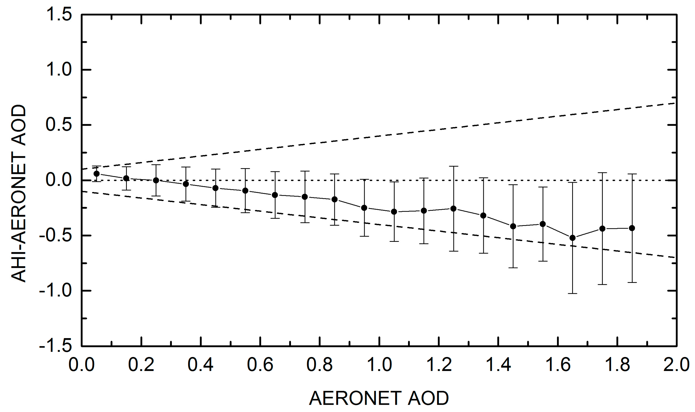
Figure 3 shows the difference between AHI and AERONET AOD as a function of AERONET AOD. The circles and vertical lines represent the mean and standard deviation for each AOD bin of size 0.1. Figure 3 reveals that with the increase of aerosol loading, the retrieved AHI AOD changes from overestimation (AOD < 0.3) to underestimation (AOD ≥ 0.3). Notably, at a lower aerosol loading (AOD < 0.3) the means of differences remain within the dashed lines, which is ± (0.1 + 0.3 × AOD), which indicates that the contribution of subpixel cloud contamination is possibly not significant for AHI AOD. In addition, as aerosol loading increases, the means of differences decrease gradually, which indicates that the performance of the algorithm deteriorates with an increase of aerosol loading. Moreover, 80% of the records fall within the dashed lines, which indicates that the expected uncertainty of AHI AOD is approximately ± (0.1 + 0.3 × AOD). Additionally, it further indicates that the AHI aerosol retrieval algorithm tends to underestimate AOD. As previously discussed, the increase in deviation with increasing AOD is mostly likely caused by the inadequate representation of the aerosol models.
3.2. Evaluation for Different Regions
To study the regional variation of the AHI AOD performance, the regional evaluation was conducted. Considering geographical distribution, climate and surface differences, it was divided into three regions: East Asia, Southeast Asia, and Australia. The linear fit statistics are shown in Table 3.
3.2.1. East Asia
There are 33 AERONET sites in East Asia, which correspond to sites 1–33 in Table 1 and Table 2. Table 2 shows that the range of correlation coefficients over East Asia is between 0.64 (Douliu) and 0.96 (Shirahama). The percentage of correlation coefficients greater than 0.7 is 85% (with 28 sites), which is better than the full disk statistic (74%). Table 3 shows that the correlation coefficient of East Asia (0.86) is higher than the full disk statistic (0.82) and better than that for other regions (0.79 and 0.35). In addition, East Asia has the largest slope (0.84), further demonstrating the better performance of the algorithm in East Asia.
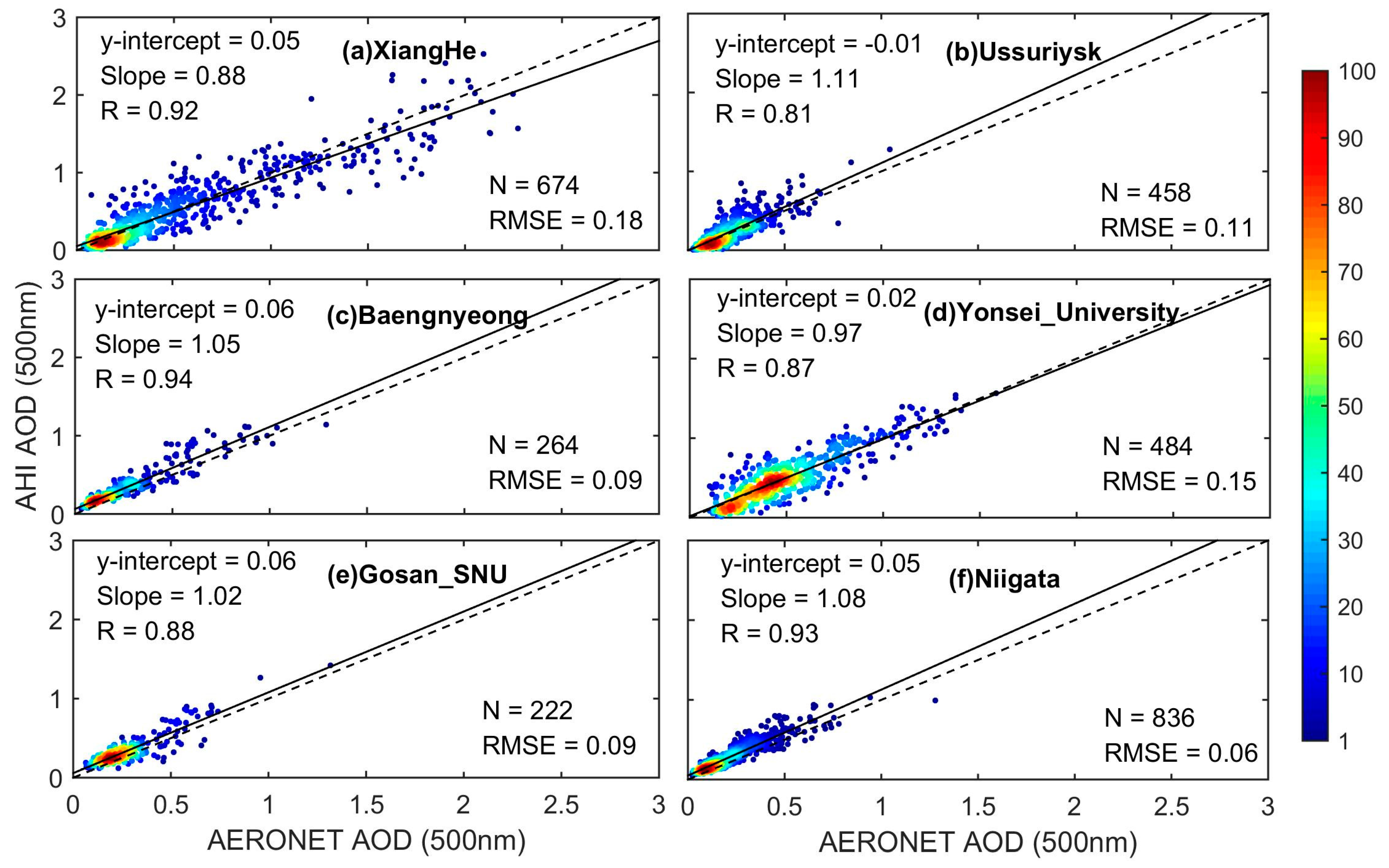
Figure 4 presents comparisons at six individual sites (XiangHe, Ussuriysk, Baengnyeong, Yonsei_University, Gosan_SNU, and Niigata) of East Asia. Figure 4 shows a good agreement between AHI and AERONET AOD at selected sites. However, underestimation can be observed at XiangHe and Yonsei_University, especially at AOD < 0.3.
3.2.2. Southeast Asia
Sites located in Southeast Asia include sites 40–58 in Table 1 and Table 2. Table 2 shows that the correlation coefficients vary from 0.40 (Pontianak) to 0.98 (Palangkaraya). Table 2 exhibits that, at 15 out of the 19 sites, the correlation coefficients are greater than 0.7. Furthermore, the minimum slope is 0.47. However, Table 3 shows that the correlation coefficient of Southeast Asia (0.79) is lower than the full disk statistic (0.82) and East Asia (0.86). In addition, the slope of the linear fit (0.58) is much lower than unity. Moreover, the largest MAD (0.21) and SDEV (0.19) also indicate that the AHI retrieved AOD has some deviations in Southeast Asia.
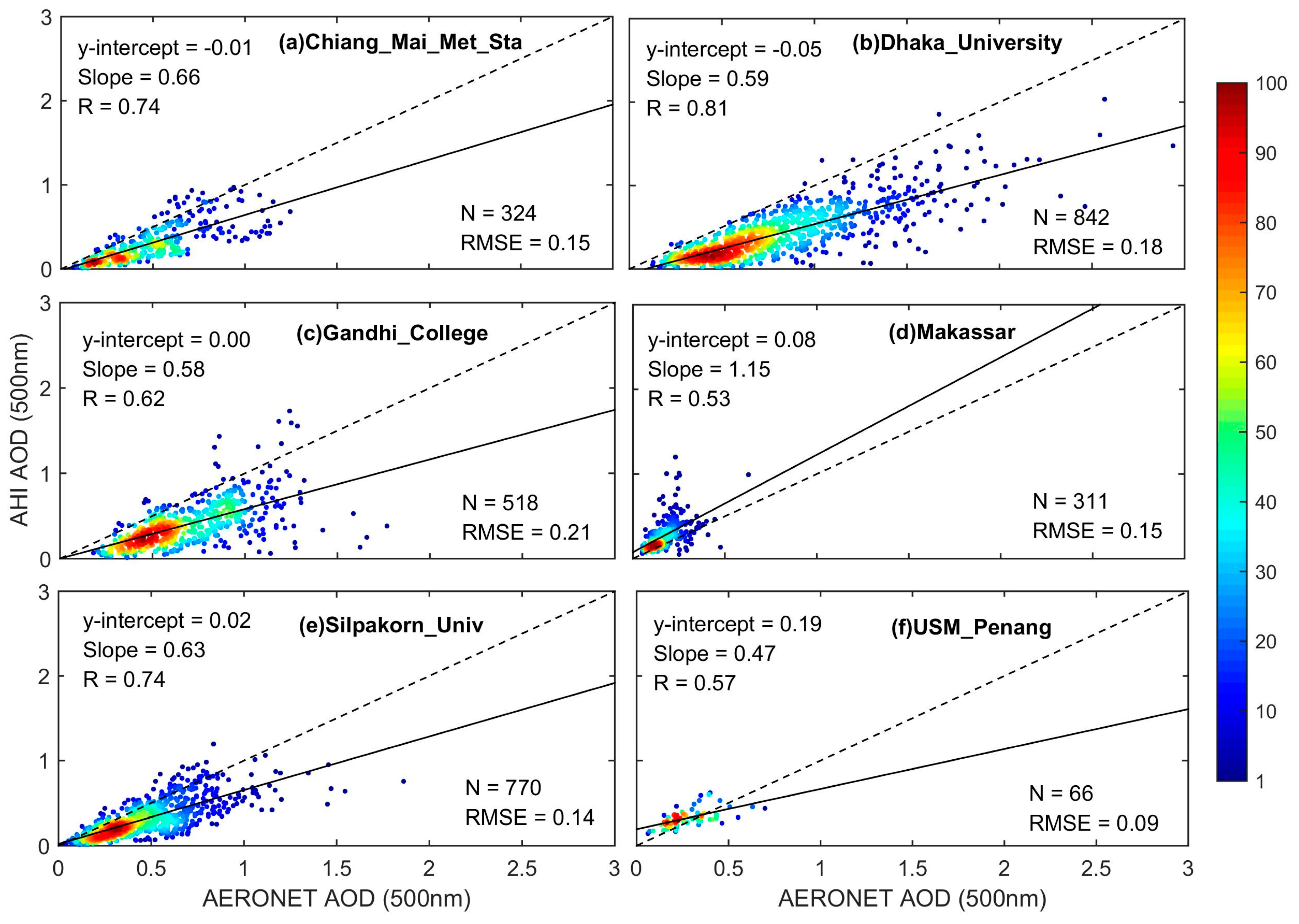
Figure 5 presents comparisons at six individual sites (Chiang_Mai_Met_Sta, Dhaka_University, Gandhi_College, Makassar, Silpakorn_Univ, and USM_Penang) in Southeast Asia. There is an obvious AOD underestimation at Chiang_Mai_Met_Sta (Figure 5a), Dhaka_University (Figure 5b), Gandhi_College (Figure 5c), and Silpakorn_Univ (Figure 5e). As discussed in Section 3.1, the underestimation may be explained by the overestimation of the surface reflectance. The rainy weather of the tropics makes it difficult to obtain cloud and aerosol clear surface reflectance. The overestimation at Makassar (Figure 5d) is possibly caused by subpixel cloud contamination.
3.2.3. Australia
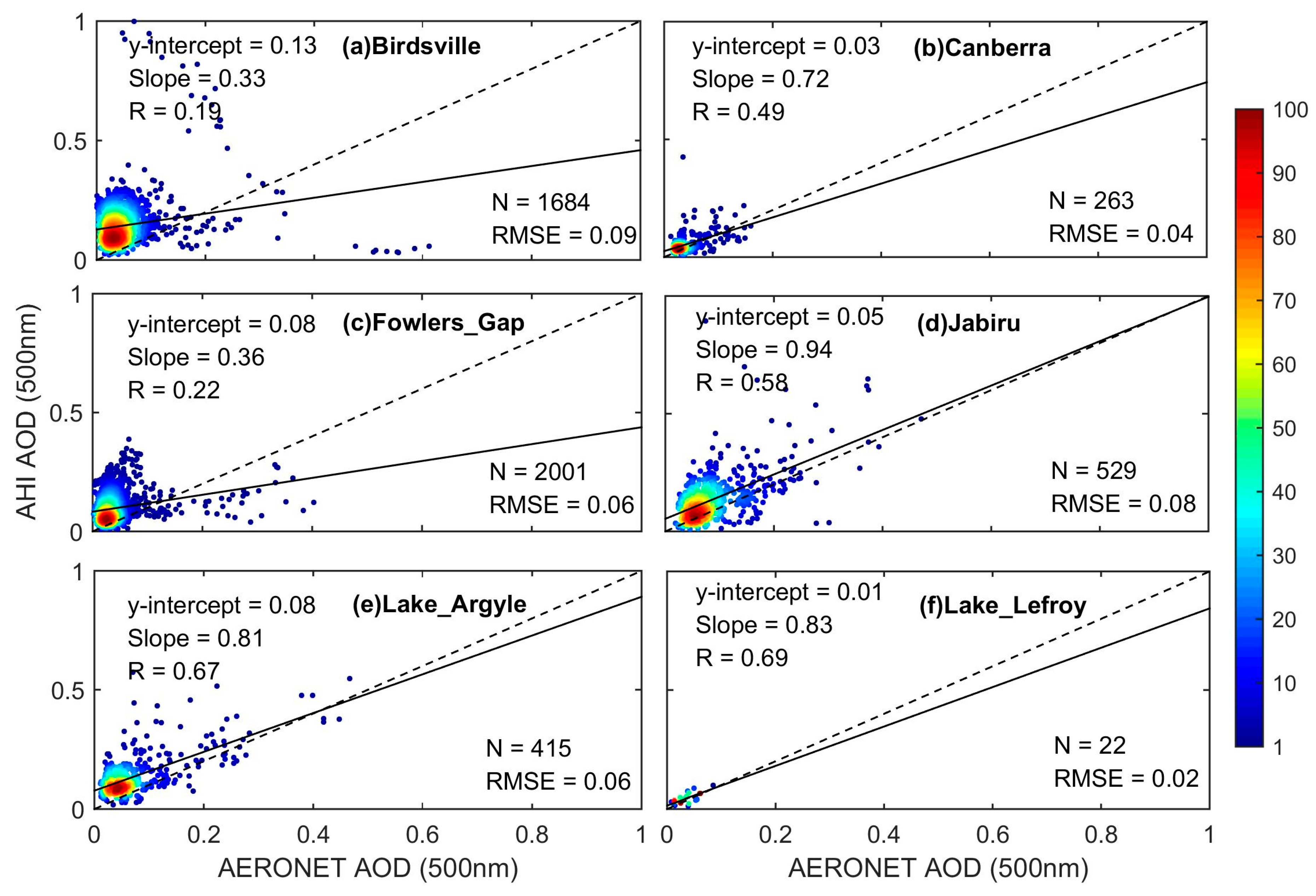
Sites 34–39 (in Table 1 and Table 2) are located in Australia. It is worth noting that all sites exhibit correlation coefficients lower than 0.7, which vary from 0.19 (Birdsville) to 0.69 (Lake_Lefroy). Additionally, Table 3 shows that the correlation coefficient and slope for the Australia sites are 0.35 and 0.57, respectively, which are much lower than those for other regions. This worse evaluation indicates that the retrieved AHI AOD has a high deviation in Australia. Hence, it should be used with caution in this region. The poor performance can be explained by bad characterization of the surface reflectance. Generally, the surface reflectance over Australia is higher than that of East Asia and Southeast Asia. Furthermore, there are two sites (Figure 6e,f) around the lakes. According to the previous discussion, the uncertainty of the surface is easily increased due to the bright surface. In addition, the poorer performance of the reflectance spectral dependence over bright surfaces makes the residual aerosol correction much more difficult. It should be noted that the sites near the water in Southeast Asia and East Asia, such as Niigata, does not show clearly poor results. Therefore, in addition to the uncertainty of the surface, the aerosol concentration is very low in Australia, which may also be one cause of poor performance in these sites. The AOD values cluster in a range of less than 0.1, with a percentage of 92%, making the agreement even worse.
Figure 6 presents comparisons at six individual sites (Birdsville, Canberra, Fowlers_Gap, Jabiru, Lake_Argyle, and Lake_Lefroy) in Australia. The overestimation is clearly observed at the AERONET AOD values of 0.1 and lower in Figure 6a,c,d,e. As discussed above, it is probably associated with subpixel cloud contamination.
3.3. Evaluation for Different Times
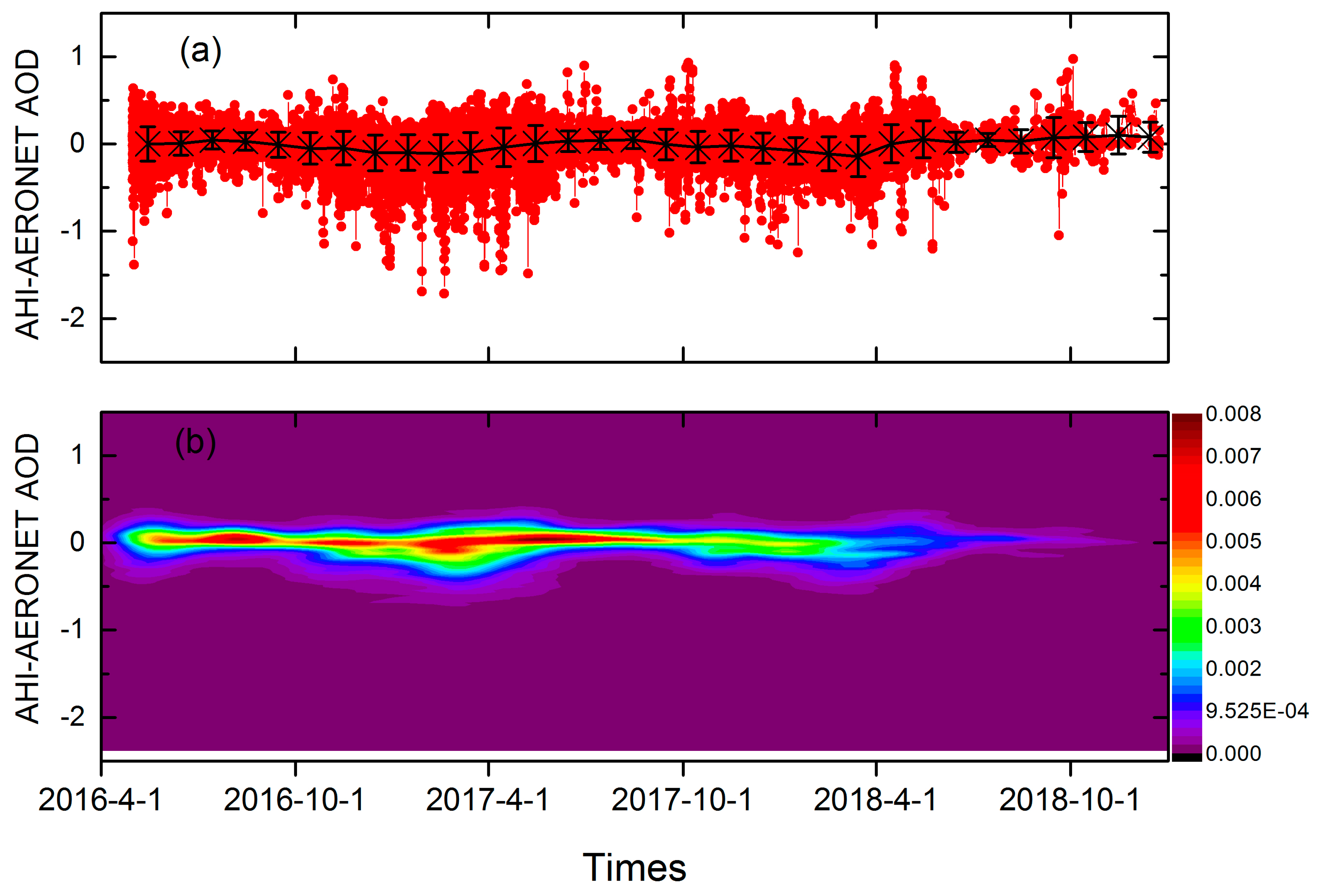
To examine the stability of the AHI aerosol product and the sensor, we plot the time series of AHI-AERONET matchups (Figure 7) and the corresponding linear fit statistics (Figure 8). Figure 7 exhibits a time series of AOD differences between AHI and AERONET. The fluctuation of differences and statistics can be clearly observed in Figure 7, but there is no sign of temporal degradation. It should be noted that the number of samples decreased due to the lack of Level 2.0 measurements for some AERONET sites since July 2018, but this does not indicate the decline of aerosol capacity observed by AHI. Consequently, the slight differences and absence of the temporal trend indicate that the quality of AHI retrieval AOD is stable from 2016 to 2018.
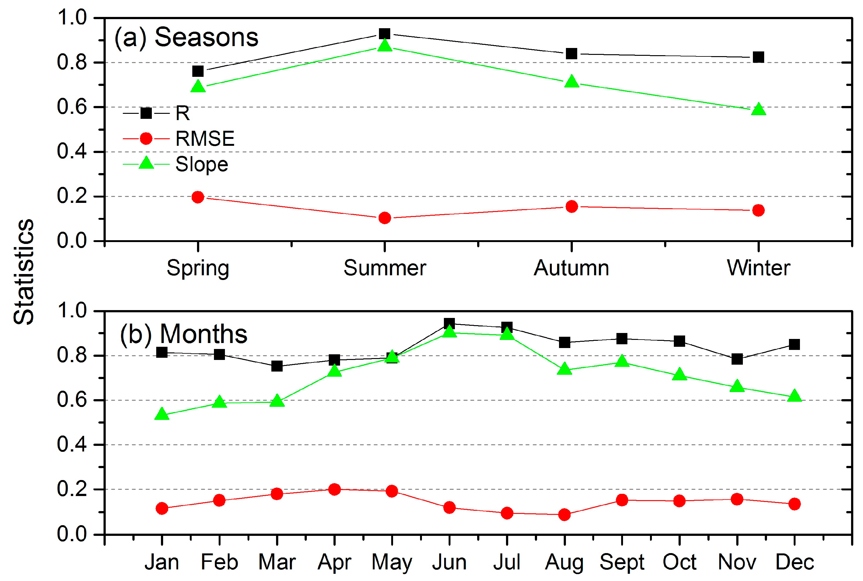
Table 4 shows the statistics of AHI-AERONET validations for different months and seasons, while Figure 8 shows the variation of statistics (R, slope, and RMSE) in Table 4. It should be noted that in this paper, spring includes Mar, Apr and May (MAM); summer includes Jun, Jul and Aug (JJA); autumn includes Sept, Oct and Nov (SON); and winter includes Dec, Jan and Feb (DJF). Figure 8 exhibits obvious seasonal and monthly variations. As the season changes from spring to winter, the correlation coefficients and slope increase first and then decrease. Table 4 shows that March has the lowest correlation coefficients (0.75), while June has the highest correlation coefficients (0.94). Furthermore, summer has the largest correlation coefficients (0.93), followed by autumn (0.84), while winter and spring have relatively lower values (0.82 and 0.76, respectively). It probably can be explained by a rapid change of surface coverage. Especially in temperate regions, where vegetation grows rapidly in April and May, causing dramatic variations in the surface reflectance. The quick variations weaken the representative of the combined surface reflectance. As in the combination algorithm (introduced in Section 2.1), it is assumed that the surface changes little within one month. The reason for the reduced performance of the AHI AOD in winter may be that the vegetation coverage is reduced, especially in the Northern Hemisphere, resulting in the increased surface reflectance. According to previous discussion, higher surface reflectance will increase uncertainty. Furthermore, snow in the winter will dramatically change the surface, making the situation worse.
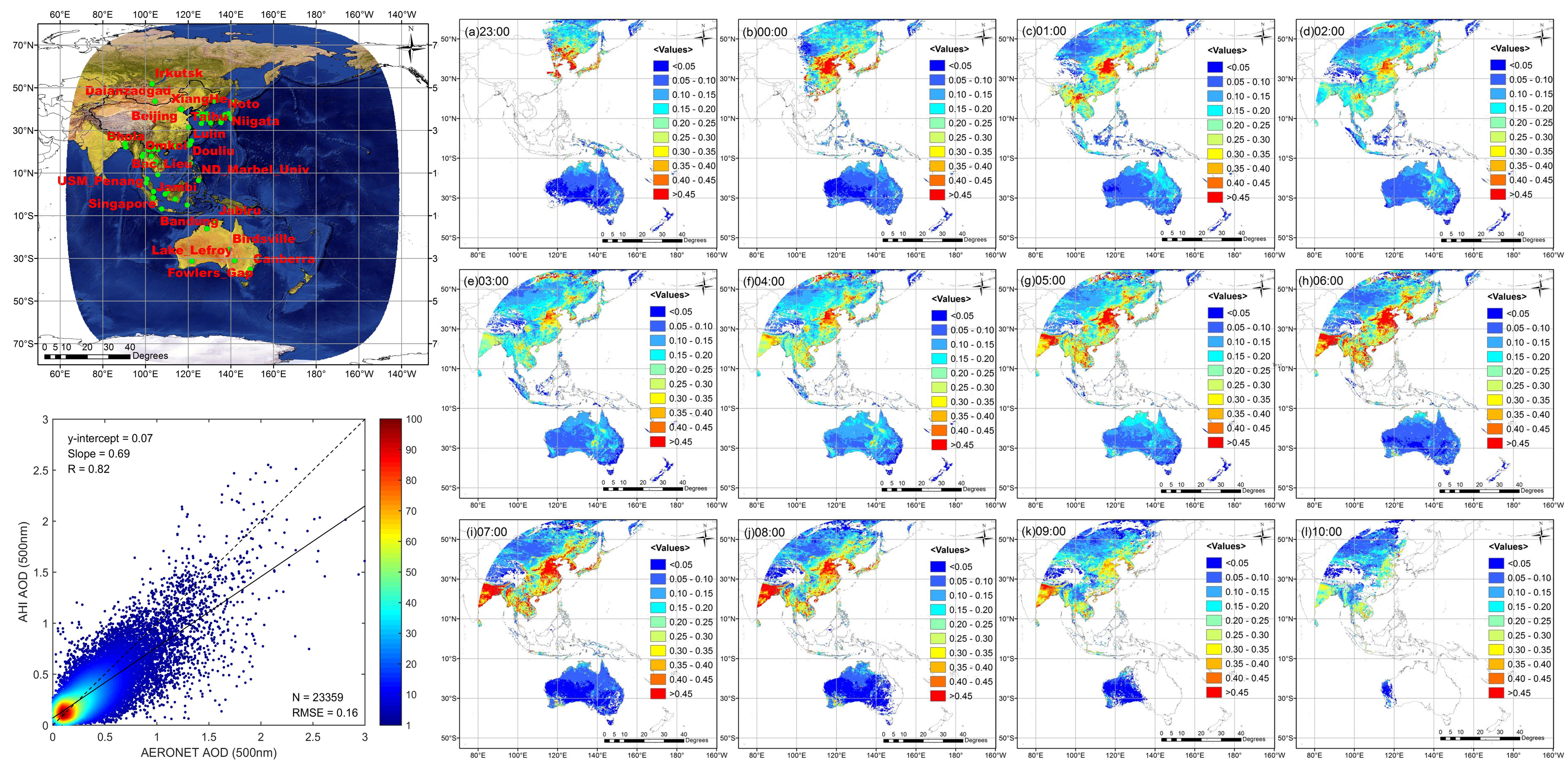
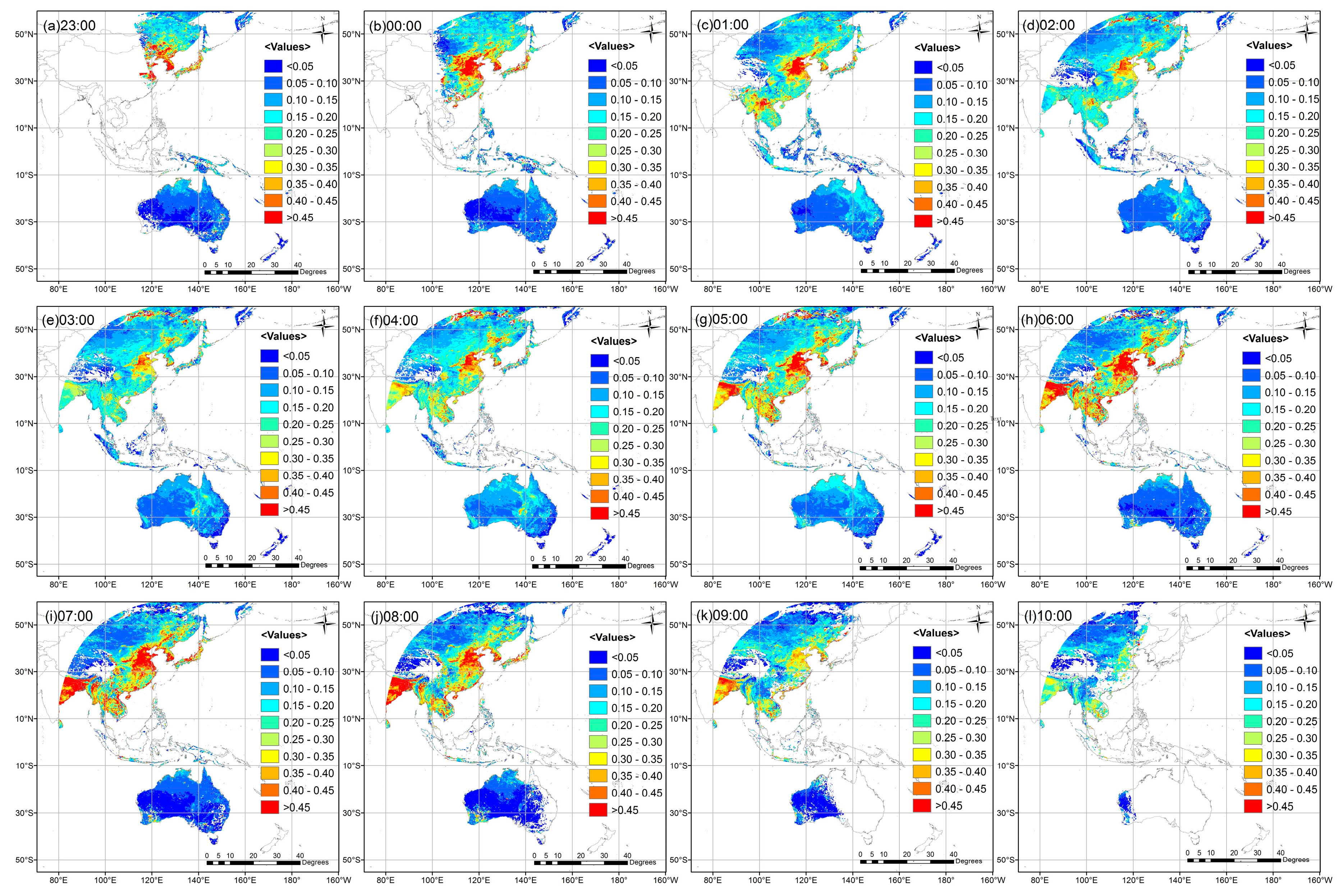
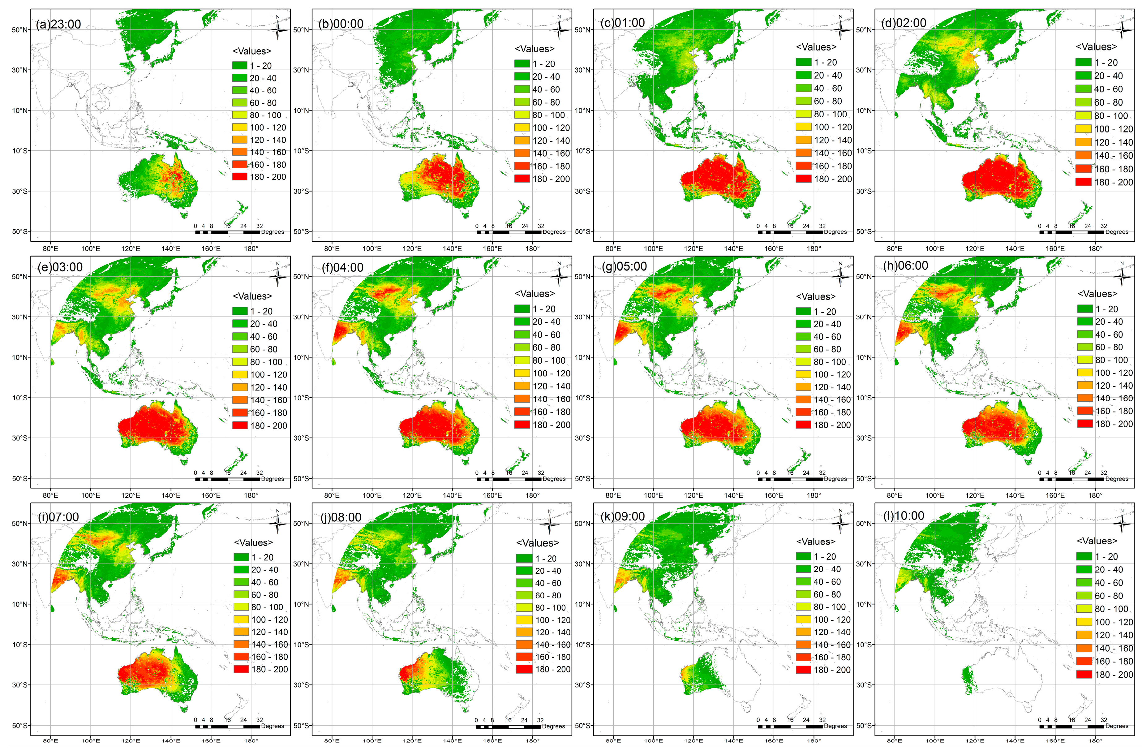
Figure 9 shows the annual average of AHI AOD over twelve hours (23:00–10:00 (Coordinated Universal Time, UTC)) in 2017, while Figure 10 shows the corresponding frequency of observations. Figure 9 shows that, for a given area, AHI can provide no less than ten times the aerosol observations (one-hour interval) in one day, which demonstrates the ability of AHI to acquire a high frequency of AOD. In Figure 10, the spatial distribution of the annual frequency displays an hourly variation. The variation can be clearly observed in Australia, where the areas with high observation frequency move from east to the west within hours. This can be explained by the fact that when the solar zenith angle increases, the surface signal weakens and the atmospheric refraction boosts, resulting in a reduced ability to retrieval aerosols.
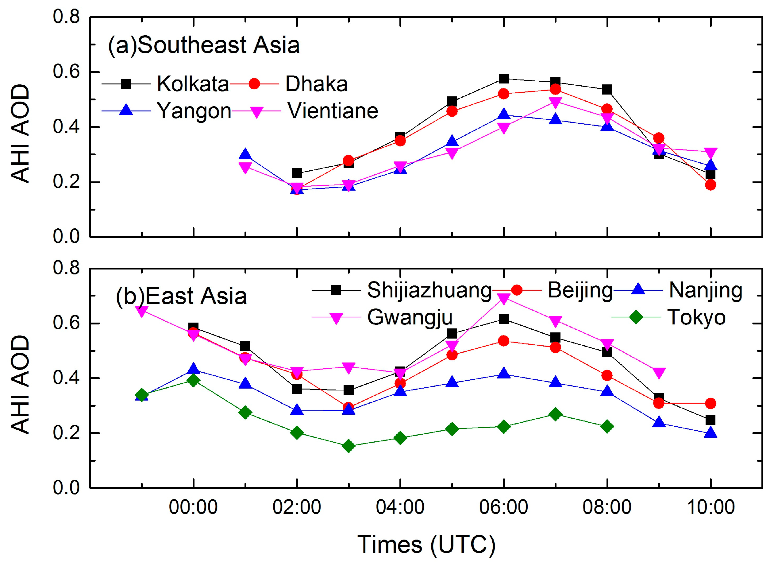
Figure 11 shows the variations in the annual average (2017) of AHI AOD on the scale of hours over different cities. The cities located in Southeast Asia (Figure 11a; Kolkata, Dhaka, Yangon, and Vientiane) and East Asia (Figure 11b; Shijiazhuang, Beijing, Nanjing, Gwangju, and Tokyo) were selected, considering their geographical distribution and representation in the region. Figure 11a shows that cities in Southeast Asia exhibit similar trends—that is, with variation in time from 01:00 to 10:00, the AOD first increases and peaks at 06:00 or 07:00 and then decreases. Figure 11b shows that AOD usually peaks at 06:00 or 07:00 in the cities of East Asia. Furthermore, there are some cities that have higher AOD values at 23:00 or 00:00. The fluctuations in Figure 11 indicate that AHI can reveal variations of aerosol with high temporal resolution.
4. Summary and Conclusions
Since its official operation in July 2015, Himawari-8 AHI has provided a large amount of aerosol observation data with high temporal resolution (10 min), which is important for monitoring aerosol in East Asia and Southeast Asia where aerosols are prevalent. However, there is still a lack of extensive evaluation of the aerosol products of AHI. In this study, the first comprehensive discussion of the applicability of AHI AOD L3 (Version 3.0) is carried out. A rigorous AOD validation analysis over nearly three years (May 2016–December 2018) was carried out. The AHI AOD and AERONET direct sun measurements were compared at 58 AERONET locations. The detailed statistics of the validation analysis are summarized in Table 2. The overall performance of the AHI AOD yields a correlation coefficient of 0.82 and an RMSE of 0.16, which indicate a good agreement between AHI and AERONET AOD. Additionally, the analysis also shows that the AHI aerosol retrieval algorithm tends to underestimate the atmospheric aerosol load (slope of 0.69). Furthermore, the underestimation increases with increasing aerosol concentration. Moreover, the uncertainty of AHI AODmerged (Level3 Version3.0) is approximately ± (0.1 + 0.3 × AOD).
To evaluate the regional performance of AHI AOD, detailed analyses over three regions (East Asia, Southeast Asia, and Australia) were carried out. The results show that the performance varies with region. East Asia has the best performance (correlation coefficient 0.86, slope 0.84, and RMSE 0.16), followed by Southeast Asia (correlation coefficient 0.79, slope 0.58, and RMSE 0.16) and Australia (correlation coefficient 0.35, slope 0.57, and RMSE 0.07).
The monthly and seasonal comparisons of AHI-AERONET were carried out to study the variation of the AHI AOD performance over time. The monthly and seasonal linear fit statistics were analyzed. The results show that summer has the best performance (correlation coefficient 0.93, slope 0.87, and RMSE 0.10), followed by autumn (correlation coefficient 0.84 slope 0.71, and RMSE 0.15), winter (correlation coefficient 0.82 slope 0.59, and RMSE 0.14), and spring (correlation coefficient 0.76 slope 0.69, and RMSE 0.2). March has the lowest performance in a 12-month period (correlation coefficient 0.75, slope 0.59, and RMSE 0.14), while the best performance appeared in June (correlation coefficient 0.94, slope 0.90, and RMSE 0.12).
In addition, the variations in the annual mean AHI AOD on the scale of hours were studied. Annual average maps of twelve consecutive hours (from 23:00 to 10:00 (UTC)) in 2017 were produced. The results suggest that AHI can provide continuous aerosol monitoring for no less than ten hours in the observation areas. Furthermore, AHI is capable of revealing high temporal aerosol variations on a large spatial scale. This analysis confirms the potential of using AHI observations as a useful remote sensing tool for AOD retrieval over land.
This work will provide a primary reference for the application of the AHI AOD product, as well as the reference for the possible update of the AOD retrieval algorithm of AHI and other geostationary satellites (Himawari-9, GOES-R, Meteosat-9, and FengYun-4A). In addition, the evaluation of AHI AOD also will provide a quantitative reference for data assimilation.
Author Contributions
W.Z. designed the research, carried out the modeling, and prepared the manuscript. L.Z. proposed the direction of research. H.X. reviewed and edited the manuscript. All authors contributed to the scientific content, the interpretation of the results, and manuscript revisions.
Funding
This paper was supported by the National Natural Science Foundation of China grant number 41801255.
Acknowledgments
This study was supported by National Natural Science Foundation of China (grant 41801255). The authors acknowledge all the AERONET investigators for maintaining CIMEL instruments and providing high quality aerosol products. We acknowledge the free use of the Himawari-8 AHI aerosol product provided by the Japan Aerospace Exploration Agency (JAXA). Data used in this paper come from the following sources: The AHI data were obtained from http://aeronet.gsfc.nasa.gov/index.html, AERONET from http://aeronet.gsfc.nasa.gov/index.html.
Conflicts of Interest
The authors declare no conflict of interest.
References
- Kaufman, Y.J.; Tanré, D.; Boucher, O. A satellite view of aerosols in the climate system. Nat. Cell Boil. 2002, 419, 215–223. [Google Scholar] [CrossRef] [PubMed]
- Adler, C.E.; Hadorn, G.H. The IPCC and treatment of uncertainties: Topics and sources of dissensus. Wiley Interdiscip. Rev. Clim. Chang. 2014, 5, 663–676. [Google Scholar] [CrossRef]
- Shine, K.P. Radiative Forcing and Climate Change. Encycl. Aerosp. Eng. 2010, 102, 6831–6864. [Google Scholar]
- Andreae, M.O.; Jones, C.D.; Cox, P.M. Strong present-day aerosol cooling implies a hot future. Nat. Cell Boil. 2005, 435, 1187–1190. [Google Scholar] [CrossRef] [PubMed]
- Seinfeld, J. Atmospheric science: Black carbon and brown clouds. Nat. Geosci. 2008, 1, 15–16. [Google Scholar] [CrossRef]
- Yu, H.; Kaufman, Y.J.; Chin, M.; Feingold, G.; Remer, L.A.; Anderson, T.L.; Balkanski, Y.; Bellouin, N.; Boucher, O.; Christopher, S.; et al. A review of measurement-based assessments of the aerosol direct radiative effect and forcing. Atmos. Chem. Phys. Discuss. 2006, 6, 613–666. [Google Scholar] [CrossRef] [Green Version]
- Anderson, T.L.; Charlson, R.J.; Schwartz, S.E.; Knutti, R.; Boucher, O.; Rodhe, H.; Heintzenberg, J. ATMOSPHERIC SCIENCE: Climate Forcing by Aerosol—A Hazy Picture. Science 2003, 300, 1103–1104. [Google Scholar] [CrossRef] [PubMed]
- Bullard, R.L.; Singh, A.; Anderson, S.M.; Lehmann, C.M.; Stanier, C.O. 10-Month characterization of the aerosol number size distribution and related air quality and meteorology at the Bondville, IL Midwestern background site. Atmos. Environ. 2017, 154, 348–361. [Google Scholar] [CrossRef]
- Binkowski, F.S.; Roselle, S.J. Models-3 Community Multiscale Air Quality (CMAQ) model aerosol component 1. Model description. J. Geophys. Res. Biogeosci. 2003, 108, 4183. [Google Scholar] [CrossRef]
- Chow, J.C.; Watson, J.G.; Fujita, E.M.; Lu, Z.; Lawson, D.R.; Ashbaugh, L.L. Temporal and spatial variations of PM2.5 and PM10 aerosol in the Southern California air quality study. Atmos. Environ. 1994, 28, 2061–2080. [Google Scholar] [CrossRef]
- Semeniuk, K.; Dastoor, A. Current state of aerosol nucleation parameterizations for air-quality and climate modeling. Atmos. Environ. 2018, 179, 77–106. [Google Scholar] [CrossRef]
- Christopher, S.A.; Wang, J. Intercomparison between satellite-derived aerosol optical thickness and PM2.5 mass: Implications for air quality studies. Geophys. Lett. 2003, 30, 2095. [Google Scholar]
- Mishchenko, M.I.; Geogdzhayev, I.V.; Cairns, B.; Carlson, B.E.; Chowdhary, J.; Lacis, A.A.; Liu, L.; Rossow, W.B.; Travis, L.D. Past, present, and future of global aerosol climatologies derived from satellite observations: A perspective. J. Quant. Spectrosc. Radiat. Transf. 2007, 106, 325–347. [Google Scholar] [CrossRef] [Green Version]
- Zhang, W.; Xu, H.; Zheng, F. Aerosol Optical Depth Retrieval over East Asia Using Himawari-8/AHI Data. Remote Sens. 2018, 10, 137. [Google Scholar] [CrossRef]
- Collins, W.D.; Rasch, P.J.; Eaton, B.E.; Khattatov, B.V.; Lamarque, J.-F.; Zender, C. Simulating aerosols using a chemical transport model with assimilation of satellite aerosol retrievals: Methodology for INDOEX. J. Geophys. Res. Biogeosci. 2001, 106, 7313–7336. [Google Scholar] [CrossRef] [Green Version]
- Ichoku, C.; Remer, L.A.; Kaufman, Y.J.; Levy, R.; Chu, D.A.; Tanré, D.; Holben, B.N. MODIS observation of aerosols and estimation of aerosol radiative forcing over southern Africa during SAFARI 2000. J. Geophys. Res. Biogeosci. 2003, 108. [Google Scholar] [CrossRef] [Green Version]
- Christopher, S.A.; Wang, J. Intercomparison between multi-angle imaging spectroradiometer (MISR) and sunphotometer aerosol optical thickness in dust source regions over China: Implications for satellite aerosol retrievals and radiative forcing calculations. Tellus B Chem. Phys. Meteorol. 2004, 56, 451–456. [Google Scholar] [CrossRef]
- Torres, O.; Ahn, C.; Chen, Z. Improvements to the OMI near-UV aerosol algorithm using A-train CALIOP and AIRS observations. Atmos. Meas. Tech. 2013, 6, 3257–3270. [Google Scholar] [CrossRef] [Green Version]
- Deuzé, J.L.; Bréon, F.M.; Devaux, C.; Goloub, P.; Herman, M.; Lafrance, B.; Maignan, F.; Marchand, A.; Nadal, F.; Perry, G.; et al. Remote sensing of aerosols over land surfaces from POLDER-ADEOS-1 polarized measurements. J. Geophys. Res. Biogeosci. 2001, 106, 4913–4926. [Google Scholar] [CrossRef] [Green Version]
- Takemura, T.; Nakajima, T.; Higurashi, A.; Ohta, S.; Sugimoto, N. Aerosol distributions and radiative forcing over the Asian Pacific region simulated by Spectral Radiation-Transport Model for Aerosol Species (SPRINTARS). J. Geophys. Res. Biogeosci. 2003, 108, 8659. [Google Scholar] [CrossRef]
- Kim, D.-H.; Kim, D.; Sohn, B.; Nakajima, T.; Takamura, T.; Takemura, T.; Choi, B.; Yoon, S. Aerosol optical properties over east Asia determined from ground-based sky radiation measurements. J. Geophys. Res. Biogeosci. 2004, 109, D02209. [Google Scholar] [CrossRef]
- Lau, W.K.M.; Kim, K.-M.; Kim, M.-K.; Lee, W.-S.; Kim, M.; Lee, W. A GCM study of effects of radiative forcing of sulfate aerosol on large scale circulation and rainfall in East Asia during boreal spring. Geophys. Lett. 2007, 34, 1–5. [Google Scholar]
- Eck, T.F.; Holben, B.N.; Dubovik, O.; Smirnov, A.; Goloub, P.; Chen, H.B.; Chatenet, B.; Gomes, L.; Zhang, X.-Y.; Tsay, S.-C.; et al. Columnar aerosol optical properties at AERONET sites in central eastern Asia and aerosol transport to the tropical mid-Pacific. J. Geophys. Res. Biogeosci. 2005, 110, 1–18. [Google Scholar] [CrossRef]
- Wang, J.; Christopher, S.A.; Brechtel, F.; Kim, J.; Schmid, B.; Redemann, J.; Russell, P.B.; Quinn, P.; Holben, B.N. Geostationary satellite retrievals of aerosol optical thickness during ACE-Asia. J. Geophys. Res. Biogeosci. 2003, 108, 8657. [Google Scholar] [CrossRef]
- Knapp, K.R.; Frouin, R.; Kondragunta, S.; Prados, A. Toward aerosol optical depth retrievals over land from GOES visible radiances: Determining surface reflectance. Int. J. Sens. 2005, 26, 4097–4116. [Google Scholar] [CrossRef]
- Knapp, K.R.; Haar, T.H.V.; Kaufman, Y.J. Aerosol optical depth retrieval from GOES-8: Uncertainty study and retrieval validation over South America. J. Geophys. Res. Biogeosci. 2002, 107, 4055. [Google Scholar] [CrossRef]
- Kim, J.; Yoon, J.; Ahn, M.H.; Sohn, B.J.; Lim, H.S. Retrieving aerosol optical depth using visible and mid-IR channels from geostationary satellite MTSAT-1R. Int. J. Sens. 2008, 29, 6181–6192. [Google Scholar] [CrossRef]
- Mei, L.; Xue, Y.; Wang, Y.; Hou, T.; Guang, J.; Li, Y.; Xu, H.; Wu, C.; He, X.; Dong, J.; et al. Prior information supported aerosol optical depth retrieval using FY2D data. In Proceedings of the 2011 IEEE International Geoscience and Remote Sensing Symposium, Vancouver, BC, Canada, 24–29 July 2011; Volume 3, pp. 2677–2680. [Google Scholar]
- Zhang, H.; Lyapustin, A.; Wang, Y.; Kondragunta, S.; Laszlo, I.; Ciren, P.; Hoff, R.M. A multi-angle aerosol optical depth retrieval algorithm for geostationary satellite data over the United States. Atmos. Chem. Phys. Discuss. 2011, 11, 11977–11991. [Google Scholar] [CrossRef] [Green Version]
- Norton, C.C.; Mosher, F.R.; Hinton, B.; Martin, D.W.; Santek, D.; Kuhlow, W. A Model for Calculating Desert Aerosol Turbidity over the Oceans from Geostationary Satellite Data. J. Appl. Meteorol. 1980, 19, 633–644. [Google Scholar] [CrossRef] [Green Version]
- Brindley, H.; Ignatov, A.; Brindley, H. Retrieval of mineral aerosol optical depth and size information from Meteosat Second Generation SEVIRI solar reflectance bands. Remote Sens. Environ. 2006, 102, 344–363. [Google Scholar] [CrossRef]
- Yumimoto, K.; Nagao, T.; Kikuchi, M.; Sekiyama, T.; Murakami, H.; Tanaka, T.; Ogi, A.; Irie, H.; Khatri, P.; Okumura, H.; et al. Aerosol data assimilation using data from Himawari-8, a next-generation geostationary meteorological satellite. Geophys. Lett. 2016, 43, 5886–5894. [Google Scholar] [CrossRef] [Green Version]
- Bessho, K.; Date, K.; Hayashi, M.; Ikeda, A.; Imai, T.; Inoue, H.; Kumagai, Y.; Miyakawa, T.; Murata, H.; Ohno, T.; et al. An Introduction to Himawari-8/9—Japan’s New-Generation Geostationary Meteorological Satellites. J. Meteorol. Soc. Jpn. Ser. II 2016, 94, 151–183. [Google Scholar] [CrossRef]
- Yan, X.; Li, Z.; Luo, N.; Shi, W.; Zhao, W.; Yang, X.; Jin, J. A minimum albedo aerosol retrieval method for the new-generation geostationary meteorological satellite Himawari-8. Atmos. Res. 2018, 207, 14–27. [Google Scholar] [CrossRef]
- Luan, Y.; Jaegle, L. Composite study of aerosol export events from East Asia and North America. Atmos. Chem. Phys. Discuss. 2013, 13, 1221–1242. [Google Scholar] [CrossRef] [Green Version]
- Zhang, W.; Xu, H.; Zheng, F. Classifying Aerosols Based on Fuzzy Clustering and Their Optical and Microphysical Properties Study in Beijing, China. Adv. Meteorol. 2017, 2017, 4197652. [Google Scholar] [CrossRef]
- Yumimoto, K.; Tanaka, T.Y.; Yoshida, M.; Kikuchi, M.; Nagao, T.M.; Murakami, H.; Maki, T. Assimilation and Forecasting Experiment for Heavy Siberian Wildfire Smoke in May 2016 with Himawari-8 Aerosol Optical Thickness. J. Meteorol. Soc. Jpn. Ser. II 2018, 96B, 133–149. [Google Scholar] [CrossRef]
- Zang, L.; Mao, F.; Guo, J.; Gong, W.; Wang, W.; Pan, Z. Estimating hourly PM1 concentrations from Himawari-8 aerosol optical depth in China. Environ. Pollut. 2018, 241, 654–663. [Google Scholar] [CrossRef] [PubMed]
- Wang, W.; Mao, F.; Du, L.; Pan, Z.; Gong, W.; Fang, S. Deriving Hourly PM2.5 Concentrations from Himawari-8 AODs over Beijing–Tianjin–Hebei in China. Remote Sens. 2017, 9, 858. [Google Scholar] [CrossRef]
- Irie, H.; Horio, T.; Damiani, A.; Nakajima, T.Y.; Takenaka, H.; Kikuchi, M.; Khatri, P.; Yumimoto, K. Importance of Himawari-8 Aerosol Products for Energy Management System. Earozoru Kenkyu 2017, 32, 95–100. [Google Scholar] [CrossRef]
- She, L.; Xue, Y.; Yang, X.; Guang, J.; Li, Y.; Che, Y.; Fan, C.; Xie, Y. Dust Detection and Intensity Estimation Using Himawari-8/AHI Observation. Remote Sens. 2018, 10, 490. [Google Scholar] [CrossRef]
- Yoshida, M.; Kikuchi, M.; Nagao, T.M.; Murakami, H.; Nomaki, T.; Higurashi, A. Common Retrieval of Aerosol Properties for Imaging Satellite Sensors. J. Meteorol. Soc. Jpn. Ser. II 2018, 96B, 193–209. [Google Scholar] [CrossRef]
- Fukuda, S.; Nakajima, T.; Takenaka, H.; Higurashi, A.; Kikuchi, N.; Nakajima, T.Y.; Ishida, H. New approaches to removing cloud shadows and evaluating the 380 nm surface reflectance for improved aerosol optical thickness retrievals from the GOSAT/TANSO-Cloud and Aerosol Imager. J. Geophys. Res. Atmos. 2013, 118, 13520–13531. [Google Scholar] [CrossRef]
- Kaufman, Y.J.; Tanre, D.; Remer, L.A.; Vermote, E.F.; Chu, A.; Holben, B.N. Operational remote sensing of tropospheric aerosol over land from EOS moderate resolution imaging spectroradiometer. J. Geophys. Res. Biogeosci. 1997, 102, 17051–17067. [Google Scholar] [CrossRef] [Green Version]
- Nakajima, T.; Tanaka, M. Matrix formulations for the transfer of solar radiation in a plane-parallel scattering atmosphere. J. Quant. Spectrosc. Radiat. Transf. 1986, 35, 13–21. [Google Scholar] [CrossRef]
- Ota, Y.; Higurashi, A.; Nakajima, T.; Yokota, T. Matrix formulations of radiative transfer including the polarization effect in a coupled atmosphere–ocean system. J. Quant. Spectrosc. Radiat. Transf. 2010, 111, 878–894. [Google Scholar] [CrossRef]
- Omar, A.H.; Won, J.; Winker, D.M.; Yoon, S.; Dubovik, O.; McCormick, M.P. Development of global aerosol models using cluster analysis of Aerosol Robotic Network (AERONET) measurements. J. Geophys. Res. Biogeosci. 2005, 110, 1–14. [Google Scholar] [CrossRef]
- Sayer, A.; Smirnov, A.; Hsu, N.C.; Holben, B.N. A pure marine aerosol model, for use in remote sensing applications. J. Geophys. Res. Biogeosci. 2012, 117, D05213. [Google Scholar] [CrossRef]
- Kikuchi, M.; Murakami, H.; Suzuki, K.; Nagao, T.M.; Higurashi, A. Improved Hourly Estimates of Aerosol Optical Thickness Using Spatiotemporal Variability Derived from Himawari-8 Geostationary Satellite. IEEE Trans. Geosci. Sens. 2018, 56, 3442–3455. [Google Scholar] [CrossRef]
- Holben, B.N.; Tanre, D.; Smirnov, A.; Eck, T.F.; Slutsker, I.; Abuhassan, N.; Newcomb, W.W.; Schafer, J.S.; Chatenet, B.; Lavenu, F.; et al. An emerging ground-based aerosol climatology: Aerosol optical depth from AERONET. J. Geophys. Res. Biogeosci. 2001, 106, 12067–12097. [Google Scholar] [CrossRef] [Green Version]
- Holben, B.N.; Eck, T.F.; Slutsker, I.; Smirnov, A.; Sinyuk, A.; Schafer, J.; Giles, D.; Dubovik, O. Aeronet’s Version 2.0 quality assurance criteria. In Proceedings of the SPIE Asia-Pacific Remote Sensing, Goa, India, 8 December 2006; Volume 6408. [Google Scholar] [CrossRef]
- Dubovik, O.; Smirnov, A.; Holben, B.N.; King, M.D.; Kaufman, Y.J.; Eck, T.F.; Slutsker, I. Accuracy assessments of aerosol optical properties retrieved from Aerosol Robotic Network (AERONET) Sun and sky radiance measurements. J. Geophys. Res. Atmos. 2000, 105, 9791–9806. [Google Scholar] [CrossRef] [Green Version]
- Zhang, W.; Gu, X.; Xu, H.; Yu, T.; Zheng, F. Assessment of OMI near-UV aerosol optical depth over Central and East Asia. J. Geophys. Res. Atmos. 2016, 121, 382–398. [Google Scholar] [CrossRef]
- Li, Z.; Niu, F.; Lee, K.-H.; Xin, J.; Hao, W.-M.; Nordgren, B.; Wang, Y.; Wang, P. Validation and understanding of Moderate Resolution Imaging Spectroradiometer aerosol products (C5) using ground-based measurements from the handheld Sun photometer network in China. J. Geophys. Res. Biogeosci. 2007, 112. [Google Scholar] [CrossRef] [Green Version]
- Levy, R.; Remer, L.A.; Kleidman, R.G.; Mattoo, S.; Ichoku, C.; Kahn, R.; Eck, T.F. Global evaluation of the Collection 5 MODIS dark-target aerosol products over land. Atmos. Chem. Phys. Discuss. 2010, 10, 10399–10420. [Google Scholar] [CrossRef] [Green Version]
- Hsu, N.C.; Jeong, M.-J.; Bettenhausen, C.; Sayer, A.; Hansell, R.; Seftor, C.S.; Huang, J.; Tsay, S.-C. Enhanced Deep Blue aerosol retrieval algorithm: The second generation. J. Geophys. Res. Atmos. 2013, 118, 9296–9315. [Google Scholar] [CrossRef] [Green Version]
- Hsu, N.; Tsay, S.-C.; King, M.; Herman, J. Aerosol Properties Over Bright-Reflecting Source Regions. IEEE Trans. Geosci. Sens. 2004, 42, 557–569. [Google Scholar] [CrossRef] [Green Version]
- Ahn, C.; Torres, O.; Jethva, H. Assessment of OMI near-UV aerosol optical depth over land. J. Geophys. Res. Atmos. 2014, 119, 2457–2473. [Google Scholar] [CrossRef] [Green Version]
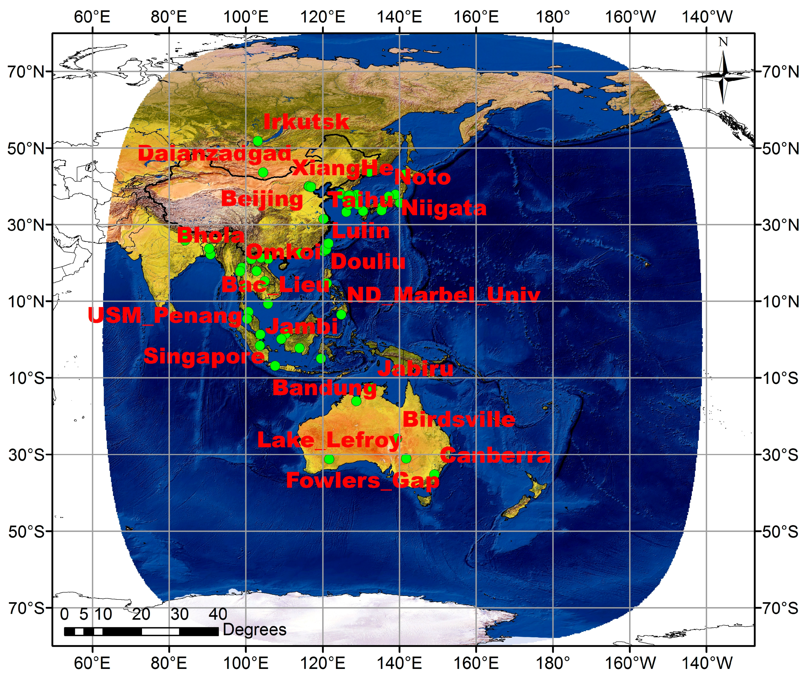
Figure 1.
The locations of the selected 58 Aerosol Robotic Network (AERONET) sites used for comparisons of Advanced Himawari Imager-Aerosol Robotic Network aerosol optical depth (AHI-AERONET AOD). The elliptical area indicates the observation range of the Himawari-8. The information for each site is presented in Table 1.

Figure 2.
The comparisons between AHI and AERONET AOD for 58 sites (May 2016–December 2018). The thick line represents linear fit. The dashed line indicates the one-to-one line.
Figure 2.
The comparisons between AHI and AERONET AOD for 58 sites (May 2016–December 2018). The thick line represents linear fit. The dashed line indicates the one-to-one line.

Figure 3.
The difference in AOD between AHI and AERONET as a function of AERONET AOD. The circles are the means of differences for each AOD bin of size 0.1, whereas the vertical lines are the associated standard deviations. The dashed lines are ± (0.1 + 0.3 × AOD).
Figure 3.
The difference in AOD between AHI and AERONET as a function of AERONET AOD. The circles are the means of differences for each AOD bin of size 0.1, whereas the vertical lines are the associated standard deviations. The dashed lines are ± (0.1 + 0.3 × AOD).

Figure 4.
AOD comparisons between AHI and AERONET for sites in East Asia. The thick line represents the linear fit. The dashed line indicates the one-to-one line. (a) XiangHe; (b) Ussuriysk; (c) Baengnyeong; (d) Yonsei_University; (e) Gosan_SNU; (f) Niigata.
Figure 4.
AOD comparisons between AHI and AERONET for sites in East Asia. The thick line represents the linear fit. The dashed line indicates the one-to-one line. (a) XiangHe; (b) Ussuriysk; (c) Baengnyeong; (d) Yonsei_University; (e) Gosan_SNU; (f) Niigata.

Figure 5.
The comparisons between AHI and AERONET AOD for sites at Southeast Asia. The thick line represents the linear fit. The dashed line indicates the one-to-one line. (a) Chiang_Mai_Met_Sta; (b) Dhaka_University; (c) Gandhi_College; (d) Makassar; (e) Silpakorn_Univ; (f) USM_Penang.
Figure 5.
The comparisons between AHI and AERONET AOD for sites at Southeast Asia. The thick line represents the linear fit. The dashed line indicates the one-to-one line. (a) Chiang_Mai_Met_Sta; (b) Dhaka_University; (c) Gandhi_College; (d) Makassar; (e) Silpakorn_Univ; (f) USM_Penang.

Figure 6.
AOD comparisons between AHI and AERONET for sites at Australia. The thick line represents the linear fit; the dashed line indicates the one-to-one line. (a) Birdsville; (b) Canberra; (c) Fowlers_Gap; (d) Jabiru; (e) Lake_Argyle; (f) Lake_Lefroy.
Figure 6.
AOD comparisons between AHI and AERONET for sites at Australia. The thick line represents the linear fit; the dashed line indicates the one-to-one line. (a) Birdsville; (b) Canberra; (c) Fowlers_Gap; (d) Jabiru; (e) Lake_Argyle; (f) Lake_Lefroy.

Figure 7.
Time series of AOD differences (AHI-AERONET). (a) The red points are the AOD differences. The black crosses are the means of differences for one month, whereas the vertical lines are the associated standard deviations; (b) the density of AOD differences.
Figure 7.
Time series of AOD differences (AHI-AERONET). (a) The red points are the AOD differences. The black crosses are the means of differences for one month, whereas the vertical lines are the associated standard deviations; (b) the density of AOD differences.

Figure 8.
The variation in statistics (RMSE, y intercept, and R) of AHI-AERONET AOD comparison. (a) Seasons (spring: Mar, Apr and May; Summer: Jun, Jul and Aug; autumn: Sept, Oct and Nov; winter: Dec, Jan and Feb); (b) months.
Figure 8.
The variation in statistics (RMSE, y intercept, and R) of AHI-AERONET AOD comparison. (a) Seasons (spring: Mar, Apr and May; Summer: Jun, Jul and Aug; autumn: Sept, Oct and Nov; winter: Dec, Jan and Feb); (b) months.

Figure 9.
Annual average of AHI AOD for different hours in 2017. (a) 23:00; (b) 00:00; (c) 01:00; (d) 02:00; (e) 03:00; (f) 04:00; (g) 05:00; (h) 06:00; (i) 07:00; (j) 08:00; (k) 09:00; (l) 10:00 (UTC).
Figure 9.
Annual average of AHI AOD for different hours in 2017. (a) 23:00; (b) 00:00; (c) 01:00; (d) 02:00; (e) 03:00; (f) 04:00; (g) 05:00; (h) 06:00; (i) 07:00; (j) 08:00; (k) 09:00; (l) 10:00 (UTC).

Figure 10.
Annual frequency of AHI AOD for different hours in 2017. (a) 23:00; (b) 00:00; (c) 01:00; (d) 02:00; (e) 03:00; (f) 04:00; (g) 05:00; (h) 06:00; (i) 07:00; (j) 08:00; (k) 09:00; (l) 10:00 (UTC).
Figure 10.
Annual frequency of AHI AOD for different hours in 2017. (a) 23:00; (b) 00:00; (c) 01:00; (d) 02:00; (e) 03:00; (f) 04:00; (g) 05:00; (h) 06:00; (i) 07:00; (j) 08:00; (k) 09:00; (l) 10:00 (UTC).

Figure 11.
The variation in annual mean AHI AOD on the scale of hours in 2017. (a) Cities in Southeast Asia; (b) cities in East Asia.
Figure 11.
The variation in annual mean AHI AOD on the scale of hours in 2017. (a) Cities in Southeast Asia; (b) cities in East Asia.


Table 1.
Information on the selected AERONET sites.
| AERONET Sites | Longitude (Degree) | Latitude (Degree) | Elevation (m) | |
|---|---|---|---|---|
| 1 | Beijing-CAMS | 116.317 | 39.933 | 106 |
| 2 | Beijing | 116.381 | 39.977 | 92 |
| 3 | XiangHe | 116.962 | 39.754 | 36 |
| 4 | Taihu | 120.215 | 31.421 | 20 |
| 5 | Hong_Kong_Sheung | 114.117 | 22.483 | 40 |
| 6 | Douliu | 120.545 | 23.712 | 60 |
| 7 | EPA-NCU | 121.185 | 24.968 | 144 |
| 8 | Taipei_CWB | 121.500 | 25.030 | 26 |
| 9 | Lulin | 120.874 | 23.469 | 2868 |
| 10 | Chiayi | 120.496 | 23.496 | 27 |
| 11 | Chen-Kung_Univ | 120.217 | 23.000 | 50 |
| 12 | Irkutsk | 103.087 | 51.800 | 670 |
| 13 | Ussuriysk | 132.163 | 43.700 | 280 |
| 14 | Dalanzadgad | 104.419 | 43.577 | 1470 |
| 15 | Hokkaido_University | 141.341 | 43.075 | 59 |
| 16 | Niigata | 138.942 | 37.846 | 10 |
| 17 | Noto | 137.137 | 37.334 | 200 |
| 18 | Chiba_University | 140.104 | 35.625 | 60 |
| 19 | Osaka | 135.591 | 34.651 | 50 |
| 20 | Shirahama | 135.357 | 33.693 | 10 |
| 21 | Fukuoka | 130.475 | 33.524 | 30 |
| 22 | Gosan_SNU | 126.162 | 33.292 | 72 |
| 23 | Gwangju_GIST | 126.843 | 35.228 | 52 |
| 24 | KORUS_Kyungpook_NU | 128.606 | 35.890 | 65 |
| 25 | KORUS_NIER | 126.640 | 37.569 | 26 |
| 26 | KORUS_UNIST_Ulsan | 129.190 | 35.582 | 106 |
| 27 | KORUS_Baeksa | 127.569 | 37.412 | 64 |
| 28 | Anmyon | 126.330 | 36.539 | 47 |
| 29 | Gangneung_WNU | 128.867 | 37.771 | 60 |
| 30 | Hankuk_UFS | 127.266 | 37.339 | 167 |
| 31 | Seoul_SNU | 126.951 | 37.458 | 116 |
| 32 | Yonsei_University | 126.935 | 37.564 | 88 |
| 33 | Baengnyeong | 124.630 | 37.966 | 136 |
| 34 | Lake_Argyle | 128.749 | −16.108 | 150 |
| 35 | Lake_Lefroy | 121.705 | −31.255 | 300 |
| 36 | Jabiru | 132.893 | −12.661 | 30 |
| 37 | Birdsville | 139.346 | −25.899 | 46 |
| 38 | Fowlers_Gap | 141.701 | −31.086 | 181 |
| 39 | Canberra | 149.111 | −35.271 | 600 |
| 40 | Pontianak | 109.191 | 0.075 | 2 |
| 41 | Palangkaraya | 113.946 | −2.228 | 27 |
| 42 | Makassar | 119.572 | −4.998 | 16 |
| 43 | Bandung | 107.610 | −6.888 | 826 |
| 44 | USM_Penang | 100.302 | 5.358 | 51 |
| 45 | Songkhla_Met_Sta | 100.605 | 7.184 | 15 |
| 46 | Bac_Lieu | 105.730 | 9.280 | 10 |
| 47 | Silpakorn_Univ | 100.041 | 13.819 | 72 |
| 48 | Ubon_Ratchathani | 104.871 | 15.246 | 120 |
| 49 | Nong_Khai | 102.717 | 17.877 | 175 |
| 50 | Omkoi | 98.432 | 17.798 | 1120 |
| 51 | Chiang_Mai_Met_Sta | 98.972 | 18.771 | 312 |
| 52 | Luang_Namtha | 101.416 | 20.931 | 557 |
| 53 | Son_La | 103.905 | 21.332 | 683 |
| 54 | NGHIA_DO | 105.800 | 21.048 | 40 |
| 55 | Bhola | 90.750 | 22.167 | 3 |
| 56 | Dhaka_University | 90.398 | 23.728 | 34 |
| 57 | Pokhara | 83.971 | 28.151 | 807 |
| 58 | Gandhi_College | 84.128 | 25.871 | 60 |
Table 2.
Summary statistics of AHI AOD compared to AERONET AOD for different sites.
| Sites | N | MAD 1 | SE | SDEV | RMSE | y-Intercept | Slope | R | RL | RU |
|---|---|---|---|---|---|---|---|---|---|---|
| Beijing-CAMS | 1330 | 0.13 | 0.003 | 0.12 | 0.17 | 0.07 | 0.87 | 0.90 | 0.89 | 0.91 |
| Beijing | 1209 | 0.13 | 0.004 | 0.13 | 0.18 | 0.07 | 0.89 | 0.88 | 0.86 | 0.89 |
| XiangHe | 674 | 0.13 | 0.005 | 0.14 | 0.18 | 0.05 | 0.88 | 0.92 | 0.91 | 0.93 |
| Taihu | 102 | 0.13 | 0.009 | 0.09 | 0.16 | 0.04 | 0.87 | 0.81 | 0.73 | 0.86 |
| Hong_Kong_Sheung | 25 | 0.17 | 0.024 | 0.12 | 0.17 | 0.06 | 0.71 | 0.68 | 0.38 | 0.84 |
| Douliu | 269 | 0.25 | 0.012 | 0.19 | 0.17 | 0.07 | 0.47 | 0.64 | 0.56 | 0.71 |
| EPA-NCU | 429 | 0.12 | 0.005 | 0.11 | 0.12 | 0.05 | 0.71 | 0.85 | 0.82 | 0.87 |
| Taipei_CWB | 52 | 0.16 | 0.018 | 0.13 | 0.13 | 0.06 | 0.61 | 0.65 | 0.46 | 0.79 |
| Lulin | 24 | 0.04 | 0.008 | 0.04 | 0.05 | 0.00 | 1.21 | 0.83 | 0.63 | 0.92 |
| Chiayi | 630 | 0.23 | 0.005 | 0.14 | 0.14 | −0.03 | 0.66 | 0.74 | 0.70 | 0.77 |
| Chen-Kung_Univ | 1170 | 0.14 | 0.004 | 0.14 | 0.16 | 0.15 | 0.58 | 0.68 | 0.65 | 0.71 |
| Irkutsk | 184 | 0.08 | 0.006 | 0.08 | 0.07 | −0.03 | 0.83 | 0.94 | 0.92 | 0.96 |
| Ussuriysk | 458 | 0.08 | 0.004 | 0.08 | 0.11 | −0.01 | 1.11 | 0.81 | 0.78 | 0.84 |
| Dalanzadgad | 913 | 0.05 | 0.002 | 0.07 | 0.07 | −0.01 | 1.47 | 0.75 | 0.72 | 0.77 |
| Hokkaido_University | 232 | 0.15 | 0.008 | 0.12 | 0.14 | 0.06 | 1.17 | 0.93 | 0.92 | 0.95 |
| Niigata | 836 | 0.07 | 0.002 | 0.06 | 0.06 | 0.05 | 1.08 | 0.93 | 0.92 | 0.93 |
| Noto | 135 | 0.08 | 0.006 | 0.07 | 0.10 | 0.05 | 0.95 | 0.82 | 0.76 | 0.87 |
| Chiba_University | 456 | 0.09 | 0.004 | 0.09 | 0.12 | 0.06 | 1.02 | 0.78 | 0.74 | 0.82 |
| Osaka | 191 | 0.14 | 0.007 | 0.10 | 0.15 | 0.02 | 1.16 | 0.76 | 0.69 | 0.81 |
| Shirahama | 15 | 0.13 | 0.013 | 0.05 | 0.05 | 0.08 | 1.19 | 0.96 | 0.87 | 0.99 |
| Fukuoka | 34 | 0.14 | 0.019 | 0.11 | 0.16 | −0.13 | 1.40 | 0.78 | 0.61 | 0.89 |
| Gosan_SNU | 222 | 0.09 | 0.004 | 0.07 | 0.09 | 0.06 | 1.02 | 0.88 | 0.85 | 0.91 |
| Gwangju_GIST | 65 | 0.17 | 0.011 | 0.09 | 0.16 | 0.15 | 0.66 | 0.72 | 0.58 | 0.82 |
| KORUS_Kyungpook_NU | 43 | 0.16 | 0.016 | 0.10 | 0.15 | 0.03 | 0.77 | 0.80 | 0.66 | 0.89 |
| KORUS_NIER | 81 | 0.12 | 0.008 | 0.07 | 0.10 | −0.08 | 0.97 | 0.81 | 0.71 | 0.87 |
| KORUS_UNIST_Ulsan | 41 | 0.12 | 0.012 | 0.08 | 0.14 | −0.03 | 0.97 | 0.68 | 0.48 | 0.82 |
| KORUS_Baeksa | 59 | 0.14 | 0.011 | 0.09 | 0.11 | −0.04 | 0.85 | 0.94 | 0.90 | 0.96 |
| Anmyon | 245 | 0.11 | 0.005 | 0.08 | 0.11 | 0.11 | 0.89 | 0.92 | 0.90 | 0.94 |
| Gangneung_WNU | 134 | 0.11 | 0.007 | 0.08 | 0.13 | 0.05 | 0.89 | 0.85 | 0.79 | 0.89 |
| Hankuk_UFS | 679 | 0.12 | 0.003 | 0.09 | 0.14 | −0.03 | 0.97 | 0.90 | 0.88 | 0.91 |
| Seoul_SNU | 463 | 0.12 | 0.004 | 0.09 | 0.15 | 0.01 | 0.99 | 0.87 | 0.85 | 0.89 |
| Yonsei_University | 484 | 0.12 | 0.004 | 0.09 | 0.15 | 0.02 | 0.97 | 0.87 | 0.85 | 0.89 |
| Baengnyeong | 264 | 0.09 | 0.005 | 0.08 | 0.09 | 0.06 | 1.05 | 0.94 | 0.92 | 0.95 |
| Lake_Argyle | 415 | 0.07 | 0.003 | 0.06 | 0.06 | 0.08 | 0.81 | 0.67 | 0.61 | 0.72 |
| Lake_Lefroy | 22 | 0.02 | 0.002 | 0.01 | 0.02 | 0.01 | 0.83 | 0.69 | 0.39 | 0.86 |
| Jabiru | 529 | 0.06 | 0.003 | 0.07 | 0.08 | 0.05 | 0.94 | 0.58 | 0.52 | 0.63 |
| Birdsville | 1684 | 0.11 | 0.002 | 0.09 | 0.09 | 0.13 | 0.33 | 0.19 | 0.14 | 0.23 |
| Fowlers_Gap | 2001 | 0.07 | 0.001 | 0.05 | 0.06 | 0.08 | 0.36 | 0.22 | 0.18 | 0.26 |
| Canberra | 263 | 0.02 | 0.002 | 0.03 | 0.04 | 0.03 | 0.72 | 0.49 | 0.39 | 0.57 |
| Pontianak | 89 | 0.11 | 0.010 | 0.10 | 0.12 | 0.12 | 0.75 | 0.40 | 0.21 | 0.56 |
| Palangkaraya | 79 | 0.12 | 0.006 | 0.06 | 0.06 | −0.11 | 0.96 | 0.98 | 0.97 | 0.99 |
| Makassar | 311 | 0.12 | 0.008 | 0.14 | 0.15 | 0.08 | 1.15 | 0.53 | 0.45 | 0.61 |
| Bandung | 94 | 0.14 | 0.011 | 0.10 | 0.07 | 0.03 | 0.47 | 0.73 | 0.62 | 0.81 |
| USM_Penang | 66 | 0.10 | 0.008 | 0.07 | 0.09 | 0.19 | 0.47 | 0.57 | 0.38 | 0.72 |
| Songkhla_Met_Sta | 195 | 0.08 | 0.005 | 0.07 | 0.09 | 0.09 | 0.81 | 0.78 | 0.71 | 0.83 |
| Bac_Lieu | 68 | 0.08 | 0.009 | 0.08 | 0.10 | 0.01 | 0.78 | 0.81 | 0.70 | 0.88 |
| Silpakorn_Univ | 770 | 0.17 | 0.005 | 0.15 | 0.14 | 0.02 | 0.63 | 0.74 | 0.71 | 0.77 |
| Ubon_Ratchathani | 26 | 0.34 | 0.030 | 0.15 | 0.12 | -0.09 | 0.61 | 0.80 | 0.60 | 0.91 |
| Nong_Khai | 452 | 0.18 | 0.008 | 0.18 | 0.16 | 0.01 | 0.67 | 0.84 | 0.81 | 0.87 |
| Omkoi | 637 | 0.07 | 0.003 | 0.07 | 0.07 | 0.02 | 0.74 | 0.90 | 0.88 | 0.91 |
| Chiang_Mai_Met_Sta | 324 | 0.20 | 0.008 | 0.15 | 0.15 | -0.01 | 0.66 | 0.74 | 0.69 | 0.79 |
| Luang_Namtha | 241 | 0.24 | 0.012 | 0.19 | 0.09 | -0.03 | 0.56 | 0.92 | 0.90 | 0.94 |
| Son_La | 51 | 0.24 | 0.017 | 0.12 | 0.10 | -0.08 | 0.70 | 0.92 | 0.86 | 0.95 |
| NGHIA_DO | 54 | 0.17 | 0.015 | 0.11 | 0.13 | -0.10 | 0.89 | 0.94 | 0.90 | 0.97 |
| Bhola | 585 | 0.22 | 0.007 | 0.16 | 0.19 | -0.08 | 0.82 | 0.81 | 0.79 | 0.84 |
| Dhaka_University | 842 | 0.39 | 0.009 | 0.25 | 0.18 | -0.05 | 0.59 | 0.81 | 0.79 | 0.83 |
| Pokhara | 846 | 0.20 | 0.006 | 0.17 | 0.14 | -0.05 | 0.69 | 0.88 | 0.86 | 0.89 |
| Gandhi_College | 518 | 0.31 | 0.009 | 0.21 | 0.21 | 0.00 | 0.58 | 0.62 | 0.56 | 0.67 |
| Total | 23310 | 0.13 | 0.001 | 0.14 | 0.16 | 0.07 | 0.69 | 0.82 | 0.81 | 0.82 |
1 MAD represents the mean absolute difference. SDEV represents the standard deviation. SE presents the standard error. RMSE represents the root mean square error. R represents the correlation coefficient. RL and RU are the lower and upper bounds for a 95% confidence interval for each correlation coefficient.
Table 3.
Summary statistics of AHI AOD compared to AERONET AOD for different areas 1.
| Areas | N | MAD | SE | SDEV | RMSE | y-Intercept | Slope | R | RL | RU |
|---|---|---|---|---|---|---|---|---|---|---|
| East Asia | 12148 | 0.12 | 0.001 | 0.12 | 0.16 | 0.06 | 0.84 | 0.86 | 0.85 | 0.86 |
| Southeast Asia | 6248 | 0.21 | 0.002 | 0.19 | 0.16 | 0.04 | 0.58 | 0.79 | 0.78 | 0.80 |
| Australia | 4914 | 0.08 | 0.001 | 0.07 | 0.08 | 0.09 | 0.57 | 0.35 | 0.33 | 0.38 |
1 The meaning of each item is the same as in Table 2.
Table 4.
Summary statistics of AHI AOD compared to AERONET AOD for different months 1.
| Months | N | MAD | SE | SDEV | RMSE | y-Intercept | Slope | R | RL | RU |
|---|---|---|---|---|---|---|---|---|---|---|
| Month | ||||||||||
| January | 1788 | 0.14 | 0.004 | 0.15 | 0.12 | 0.05 | 0.53 | 0.81 | 0.80 | 0.83 |
| February | 2266 | 0.17 | 0.003 | 0.16 | 0.15 | 0.06 | 0.59 | 0.80 | 0.79 | 0.82 |
| March | 2596 | 0.19 | 0.003 | 0.17 | 0.18 | 0.08 | 0.59 | 0.75 | 0.74 | 0.77 |
| April | 1951 | 0.15 | 0.004 | 0.16 | 0.20 | 0.10 | 0.73 | 0.78 | 0.76 | 0.80 |
| May | 3164 | 0.15 | 0.002 | 0.14 | 0.19 | 0.09 | 0.79 | 0.79 | 0.78 | 0.80 |
| June | 1729 | 0.09 | 0.002 | 0.09 | 0.12 | 0.05 | 0.90 | 0.94 | 0.94 | 0.95 |
| July | 1608 | 0.08 | 0.002 | 0.07 | 0.10 | 0.06 | 0.89 | 0.93 | 0.92 | 0.93 |
| August | 1784 | 0.08 | 0.002 | 0.08 | 0.09 | 0.08 | 0.74 | 0.86 | 0.85 | 0.87 |
| September | 1196 | 0.11 | 0.004 | 0.13 | 0.15 | 0.07 | 0.77 | 0.88 | 0.86 | 0.89 |
| October | 1518 | 0.12 | 0.004 | 0.14 | 0.15 | 0.06 | 0.71 | 0.86 | 0.85 | 0.88 |
| November | 1920 | 0.14 | 0.003 | 0.14 | 0.16 | 0.07 | 0.66 | 0.78 | 0.77 | 0.80 |
| December | 1839 | 0.13 | 0.004 | 0.16 | 0.14 | 0.06 | 0.61 | 0.85 | 0.84 | 0.86 |
| Seasons | ||||||||||
| Spring | 7711 | 0.16 | 0.002 | 0.16 | 0.20 | 0.09 | 0.69 | 0.76 | 0.75 | 0.77 |
| Summer | 5121 | 0.08 | 0.001 | 0.08 | 0.10 | 0.06 | 0.87 | 0.93 | 0.92 | 0.93 |
| Autumn | 4634 | 0.13 | 0.002 | 0.14 | 0.15 | 0.07 | 0.71 | 0.84 | 0.83 | 0.85 |
| Winter | 5893 | 0.15 | 0.002 | 0.16 | 0.14 | 0.06 | 0.59 | 0.82 | 0.82 | 0.83 |
1 The meaning of each item is the same as in Table 2.
© 2019 by the authors. Licensee MDPI, Basel, Switzerland. This article is an open access article distributed under the terms and conditions of the Creative Commons Attribution (CC BY) license (http://creativecommons.org/licenses/by/4.0/).
Share and Cite
MDPI and ACS Style
Zhang, W.; Xu, H.; Zhang, L. Assessment of Himawari-8 AHI Aerosol Optical Depth Over Land. Remote Sens. 2019, 11, 1108. https://0-doi-org.brum.beds.ac.uk/10.3390/rs11091108
AMA Style
Zhang W, Xu H, Zhang L. Assessment of Himawari-8 AHI Aerosol Optical Depth Over Land. Remote Sensing. 2019; 11(9):1108. https://0-doi-org.brum.beds.ac.uk/10.3390/rs11091108
Chicago/Turabian StyleZhang, Wenhao, Hui Xu, and Lili Zhang. 2019. "Assessment of Himawari-8 AHI Aerosol Optical Depth Over Land" Remote Sensing 11, no. 9: 1108. https://0-doi-org.brum.beds.ac.uk/10.3390/rs11091108
Note that from the first issue of 2016, this journal uses article numbers instead of page numbers. See further details here.