Kernel Joint Sparse Representation Based on Self-Paced Learning for Hyperspectral Image Classification

Hubei Key Laboratory of Applied Mathematics, Faculty of Mathematics and Statistics, Hubei University, Wuhan 430062, China
*
Author to whom correspondence should be addressed.
Remote Sens. 2019, 11(9), 1114; https://0-doi-org.brum.beds.ac.uk/10.3390/rs11091114
Submission received: 15 March 2019
/
Revised: 24 April 2019
/
Accepted: 5 May 2019
/
Published: 9 May 2019
(This article belongs to the Special Issue Image Processing and Spatial Neighbourhoods for Remote Sensing Data Analysis)
Abstract
:By means of joint sparse representation (JSR) and kernel representation, kernel joint sparse representation (KJSR) models can effectively model the intrinsic nonlinear relations of hyperspectral data and better exploit spatial neighborhood structure to improve the classification performance of hyperspectral images. However, due to the presence of noisy or inhomogeneous pixels around the central testing pixel in the spatial domain, the performance of KJSR is greatly affected. Motivated by the idea of self-paced learning (SPL), this paper proposes a self-paced KJSR (SPKJSR) model to adaptively learn weights and sparse coefficient vectors for different neighboring pixels in the kernel-based feature space. SPL strateges can learn a weight to indicate the difficulty of feature pixels within a spatial neighborhood. By assigning small weights for unimportant or complex pixels, the negative effect of inhomogeneous or noisy neighboring pixels can be suppressed. Hence, SPKJSR is usually much more robust. Experimental results on Indian Pines and Salinas hyperspectral data sets demonstrate that SPKJSR is much more effective than traditional JSR and KJSR models.
1. Introduction
Hyperspectral sensors simultaneously acquire digital images in many narrow and contiguous spectral bands across a wide range of the spectrum. The resulting hyperspectral data contains both detailed spectral characteristics and rich spatial structure information from a scene. Exploiting the rich spectral and spatial information, hyperspectral remote sensing has been successfully applied in many fields [1,2,3], such as agriculture, the environment, the military, etc. In most of these applications, pixels in a scene need to be classified [2,4,5]. The commonly used classifiers include spectral-based classifiers such as nearest neighbor (NN) and support vector machine (SVM), and spatial–spectral classifiers such as mathematical morphological (MM) and Markov random field (MRF) methods [2]. Compared with the spectral-based classifiers that only use spectral information, spatial–spectral classifiers use both the spectral and spatial information of a hyperspectral image (HSI) and can produce much better classification results [5,6,7,8]. Now, spatial–spectral classifiers have become the research focus [2,5].
Under the definition of spatial dependency systems [5], spatial–spectral classification methods can be approximately divided into three categories [5]: preprocessing-based classification, postprocessing-based classification, and integrated classification. In the preprocessing-based methods, spatial features are first extracted from the HSI and then used for the classification. In postprocessing-based methods, a pixel-wise classification is first conducted, and then spatial information is used to refine the previous pixel-wise classification results. The integrated methods simultaneously use the spectral and spatial information to generate an integrated classifier. In this paper, we focus on the integrated methods.
The joint sparse representation (JSR)-based classification method is a typical integrated spatial–spectral classifier [9,10,11,12,13,14,15,16,17,18]. JSR pursues a joint representation of spatial neighboring pixels in a linear and sparse representation framework. If neighboring pixels are similar, making a joint representation of each neighboring pixel can improve the reliability of sparse support estimation [17,19]. The success of the JSR model mainly lies in the follows two factors: (1) joint representation: the neighborhood pixel set is consistent, that is, pixels in a spatial neighborhood are highly similar or belong to the same class; (2) linear representation: the linear representation framework in the JSR model is coincident with the hyperspectral data characteristics. However, in practice, spatial neighborhood is likely to have inhomogeneous pixels [15], such as background, noise, and pixels from other classes, which dramatically affects the joint representation. In addition, hyperspectral data usually exhibits nonlinear characteristics [20,21,22,23], so the linear representation framework may also be unreasonable.
To alleviate the effect of noisy or inhomogeneous neighboring pixels, an intuitive and natural idea is to introduce a weight vector to discriminate neighboring pixels. The weight can be predefined as a non-local weight [10] or dynamically updated in a nearest regularized JSR (NRJSR) model [11]. Rather than weighting neighboring pixels, another method is to construct an adaptive spatial neighborhood system such that inhomogeneous neighboring pixels are precluded. The adaptive neighborhood can be constructed based on traditional image segmentation techniques [12], the superpixel segmentation method [13], and the shape-adaptive region extraction method [14]. Both the weighting method and adaptive neighborhood method improve the consistency of neighborhood pixel sets such that the joint representation framework is effective in most cases. However, all these methods are linear methods and show performance deficiency when data are not linearly separable.
Hyperspectral data are considered inherently nonlinear [23]. The nonlinearity is attributed to multiple scattering between solar radiation and targets, the variations in sun–canopy–sensor geometry, the presence of nonlinear attenuating medium (water), the heterogeneity of pixel composition, etc. [23]. To cope with the nonlinear problem, kernel-based JSR (KJSR) methods are proposed [19,24,25,26]. KJSR mainly includes two steps: projecting the original data into high-dimensional feature space using a nonlinear map and then performing JSR in the feature space. Because the data in the feature space are linear separable, the JSR model can be directly applied. In practice, it only needs to compute a kernel function between samples. Most works on the KJSR method are concentrated on the design of kernel function. The kernel functions include Gaussian kernel [24], spatial–spectral derivative-aided kernel [25], and multi-feature composite kernel [26]. Compared with the original JSR, the use of kernel methods yields a significant performance improvement [24]. However, these kernel-based JSR methods assume that neighboring pixels have equal importance and do not considered the differences of neighboring pixels in the feature space. This is obviously unreasonable when pixels in the spatial neighborhood are inhomogeneous.
To simultaneously improve the joint representation and linear representation abilities of the JSR model, we adopt a self-paced learning (SPL) strategy [27,28,29] to select feature-neighboring pixels and propose a self-paced KJSR (SPKJSR) model. In detail, a self-paced regularization term is incorporated into the KJSR model, and the resulting regularized KJSR model can simultaneously learn the weights and sparse coefficient vectors for different feature-neighboring pixels. The optimized weight vector indicates the importance of neighboring pixels. The inhomogeneous or noisy pixels are automatically assigned small weights and hence their negative effects are eliminated.
2. Self-Paced Kernel Joint Sparse Representation
2.1. Self-Paced Learning (SPL)
Given a training set , the goal of a learning algorithm is to learn a function (or simply parameter ) by solving the following minimization problem:
where is the true value, is the estimated value, and L is a loss function.
In model (1), all training samples are used to learn the parameter without considering the differences between training samples. When there exist noisy training samples or outliers, the learned function f or model parameter will be inaccurate.
Rather than using all training samples for learning, curriculum learning (CL) or self-paced learning (SPL) adopts a gradual learning strategy to select samples from easy to complex to use in training [17,27,28,29,30,31]. Both CL and SPL share a similar conceptual learning paradigm but differ in the derivation of the curriculum. A curriculum determines a sequence of training samples ranked in ascending order of learning difficulty. In CL, the curriculum is predefined by some prior knowledge and thus is problem-specific and lacks generalizations. To alleviate this problem, the self-paced learning (SPL) method incorporates curriculum updating in the process of model optimization [28]. SPL jointly optimizes the learning objective and the curriculum such that the learned model and curriculum are consistent.
For model (1), SPL simultaneously optimizes the model parameter and the weight vector by employing a self-paced regularizer:
where is a weight that indicates the difficulty of sample , and is a self-paced function. is a “model age” parameter that decides the size of the model. The parameters and in the model (2) can be solved by an alternating optimization strategy [28].
2.2. Joint Sparse Representation (JSR)
Given a set of N training samples with , we can construct a training dictionary as . For a testing pixel , we can extract its neighboring pixels in a spatial window centered at and denote them as (), where T is the number of pixels in the neighborhood.
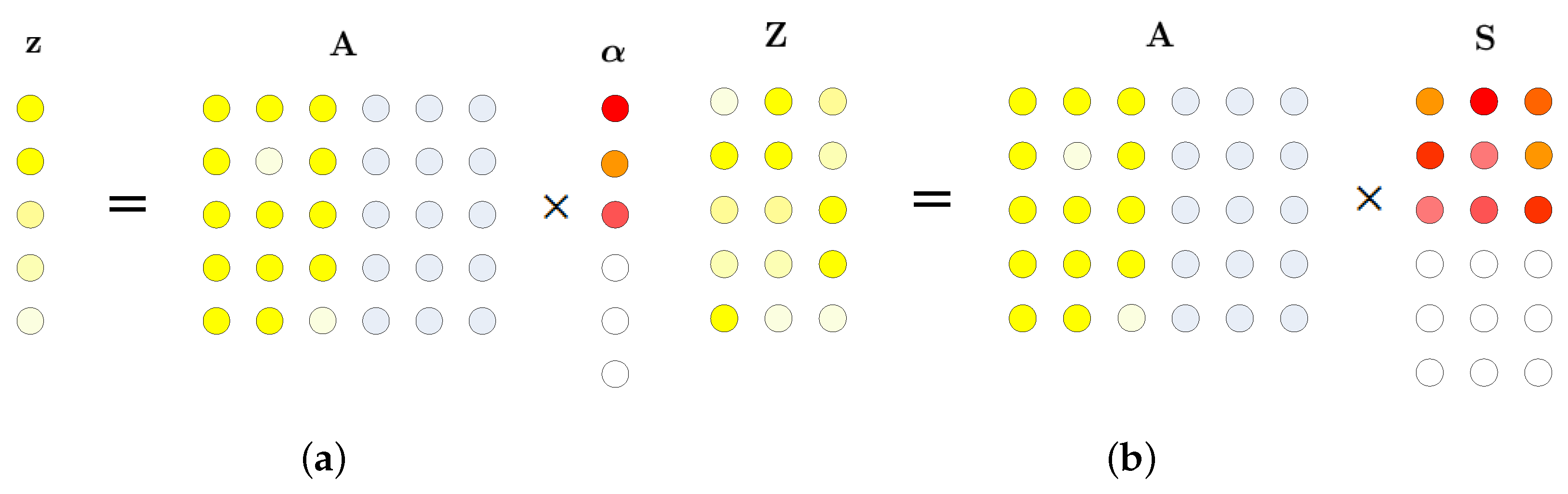
In the framework of sparse representation [32], each neighboring pixel can be represented by the training dictionary with a sparsity coefficient vector . Because neighboring pixels in a small spatial window are highly similar, they have similar representations under the training dictionary. By further assuming that the positions of nonzero elements in the sparsity coefficient vectors are the same and combining the representation of neighboring pixels, the following JSR model is generated [9]:
where is a matrix with only K nonzero rows. The sketches of sparse representation and joint sparse representation are shown in Figure 1.
The optimization problem for solving the matrix in (3) is:
where denotes the Frobenius norm, denotes the number of nonzero rows of , and K is an upper bound of the sparsity level. The solution of (4) can be obtained by the simultaneous orthogonal matching pursuit (SOMP) algorithm [9,33].
Once the row-sparse matrix is obtained, the testing pixel is classified in the class with the minimal reconstruction residual:
where the c-th residual , and is the index set corresponding to the c-th class.
2.3. Kernel Joint Sparse Representation (KJSR)
In order to exploit the intrinsic nonlinear properties of the hyperspectral imagery, pixels in the original space are projected to a high-dimensional feature space by a nonlinear map, and a kernel-based JSR (KJSR) model is obtained by performing the JSR on the feature space [24].
Denote as a nonlinear map, the KJSR model assumes that the mapped neighboring pixels in the feature space (i.e., ) are also similar and hence have a similar sparsity pattern. The KJSR model is represented as
where and D is the dimensionality of the feature space.
The optimization problem for solving the row-sparse matrix is
which can be solved by the kernel SOMP (KSOMP) algorithm [24], as shown in Algorithm 1.
| Algorithm 1 KSOMP |
| Input: Training dictionary , neighborhood pixel matrix , sparsity level K, kernel function , regularization parameter . Compute and . Set index set , and let . Run the following steps until convergence: 1 Compute the correlation coefficient matrix: 2 Identify the optimal atom, and find the corresponding index: 3 Enlarge the index set: . 4 Update the iteration number: , and go to Step 1. Output: index set and coefficient matrix . |
2.4. Self-Paced Kernel Joint Sparse Representation (SPKJSR)
In the KJSR model, it is assumed that transformed neighboring pixels have equal importance in the sparse representation. However, this assumption is usually unreasonable because there exist differences between original spatial neighboring pixels and the nonlinear map that may further enlarge the differences. The spatial inconsistency mainly appears in the following two aspects: (1) When a target pixel is around the boundary of an object, its spatial neighborhood usually contains inhomogeneous pixels, such as background pixels or pixels from different classes; (2) when a target pixel lies in the center of a large homogeneous region, all neighboring pixels are from the same class. This notwithstanding, the spatial distances between neighboring pixels and the center target pixel are different. Neighboring pixels that are far away from the center pixel usually provide limited contributions to the classification of the central target pixel, especially when the neighborhood window is large.
When there exists a spatial inconsistency between neighboring pixels, the feature representations of neighboring pixels in the kernel space are also dissimilar. Considering the distinctiveness of feature neighboring pixels, we employ a self-paced learning strategy to select important feature neighboring pixels and propose a self-paced KJSR (SPKJSR) model for the classification of HSIs.
For convenience, we first transfer the matrix-norm-based objective function in the model (7) to a vector-norm-based one as follows:
Based on the self-paced learning strategy, the SPKJSR model simultaneously optimizes a weight vector and sparse coefficient matrix for feature neighboring pixels:
where is a weight vector of feature neighboring pixels and is the self-paced function. Here, the self-paced learning strategy is used to select important feature neighboring pixels for joint sparse representation.
The optimization problem (9) can be solved by an alternative optimization strategy. With a fixed , (9) can be represented as:
where is the diagonal weight matrix.
Because , . Denote and . Then model (10) is changed to
As the feature map is unknown, we cannot compute directly. Fortunately, in the KSOMP algorithm, we only need to compute the correlation matrix between and as
By employing the KSOMP Algorithm 1, we can obtain the sparsity coefficient matrix:
and further compute the approximation error of each neighboring pixel:
Based on the approximation errors, we can describe the complexity of each feature neighboring pixel and determine the corresponding weight value based on self-paced learning as follows:
To solve the weight in (15), a self-paced function h needs to be defined. The self-paced function can be binary, linear, logarithmic, or a mixture function [28]. Here, we take the mixture function as an example to show how to solve the weight. The mixture function is defined as
Taking the derivative with respect to , we obtain the mixture weight:
Based on the weight in (18), the pixels are divided into three classes: (1) “easy” pixels with small loss () corresponding to weight 1; (2) “complex” pixels with large loss () corresponding to weight 0; and (3) “moderate” pixels whose loss is between and . It is clear that the “complex” pixels are excluded from the JSR model. When is small, only very limited “easy” pixels are used. With an increase in , more neighboring pixels are regarded as “moderate” pixels and hence used for the model.
From (18), we can see that the parameters and are related to the losses of neighboring pixels. As the amplitude of losses is different in each iteration, the setting of these parameters is difficult. Considering that and control the size of the active feature neighboring pixel set, we can set these two parameters by setting the number of feature neighboring pixels in each iteration of the self-paced learning process. For a square neighborhood with T pixels, we first define a pixel number sequence , where denotes the number of feature neighboring pixels selected in the i-th iteration [17], and . In the i-th iteration, the loss vector of neighboring pixels is sorted in an ascending order, which results in a sorted loss . Then we set the parameters as follows: with , and with . Now, the parameters and are determined by the fixed initialization parameters and step size . In the experiment, and are set as , and .
By alternatively updating the coefficient matrix and weight vector according to (13) and (15) or (18), the objective function in (11) will decrease, and finally the the algorithm will converge.
When the coefficient matrix and weight vector are obtained, the reconstruction residual for each class can be computed:
Finally, the testing pixel is assigned to the class with the minimal reconstruction residual.
Algorithm 2 shows the implementation process of SPKJSR.
| Algorithm 2 SPKJSR |
| Input: Training dictionary , neighborhood pixel matrix , sparsity level K, kernel function , the initial parameters , and step ., Compute and . Initialization: , and let . 1 Solve the coefficient matrix and weight by running the following steps until convergence: 1.1 Solve the sparsity coefficient matrix by the KSOMP algorithm: 1.2 Compute the error of each neighboring pixel: 1.3 Compute the sorted loss vector , and update the model age: 1.4 Estimate the self-paced weight: 1.5 Update the weight matrix: . 1.6 Update the number of iterations: , and go to Step 1.1. 2 Compute the reconstruct error of each class: 3 Classify the testing pixel : |
3. Experiments Results
3.1. Data Sets
To evaluate the performance of the proposed method for HSI classification, we use the following two benchmark hyperspectral data sets (available online: http://www.ehu.eus/ccwintco/index.php/Hyperspectral_Remote_Sensing_Scenes):
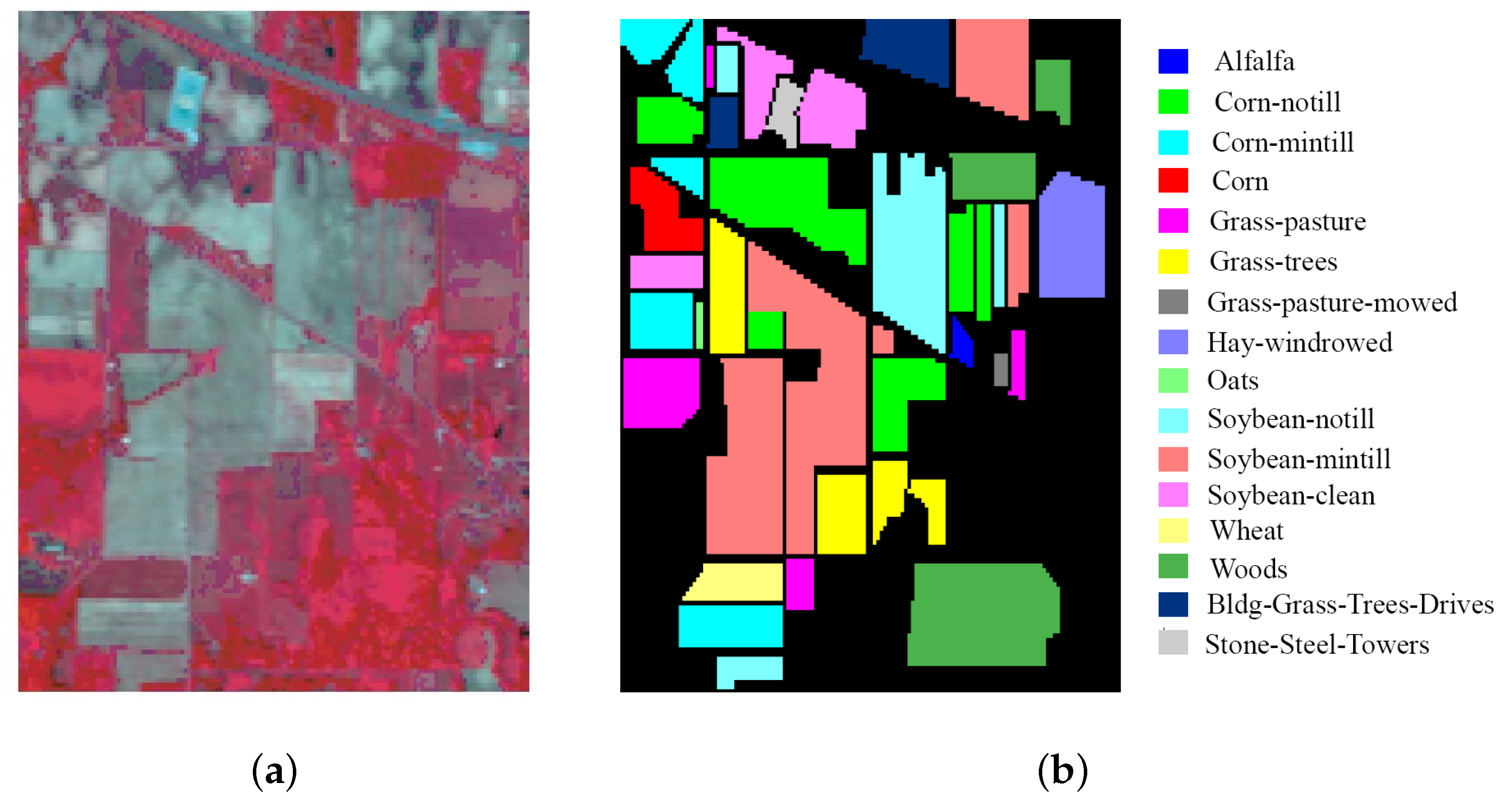
(1) Indian Pines: This image scene has a size of pixels and 220 spectral bands, where 200 spectral bands are used in the experiments by removing 20 noisy bands from the original data. The image has 16 different ground-truth classes. The false color composite image and ground-truth map are shown in Figure 2.
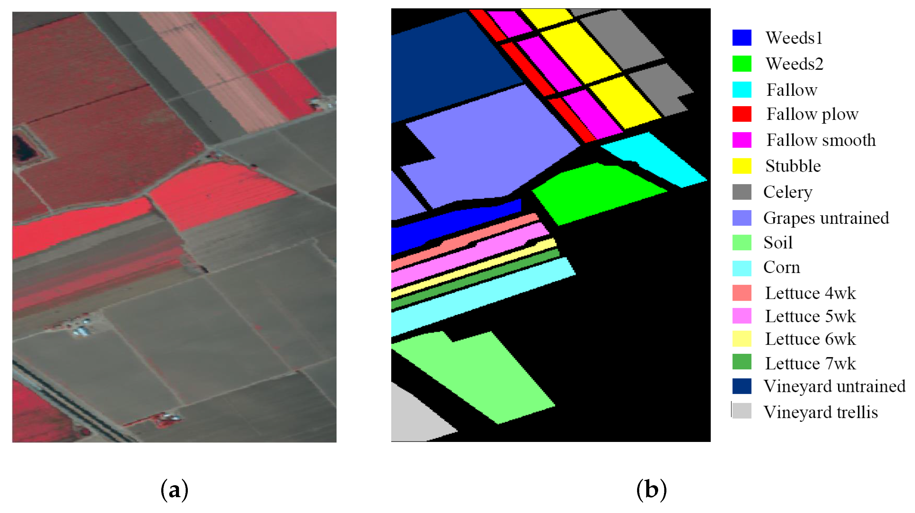
(2) Salinas: This image scene has a size of pixels and 204 spectral bands. The data contains 16 ground-truth classes and a total of 54,129 labeled samples. The false color composite image and ground-truth map are shown in Figure 3.
In real applications, the number of labeled samples is usually very limited, which makes HSI classification a challenging problem. To show the performance of our proposed method in the case of small sample sizes, we randomly choose 1% of samples from each class to form the training set, and all remaining samples consist of the testing set. The selected training and testing samples for these two data sets are shown in Table 1 and Table 2, respectively.
3.2. Model Setting
We compare the proposed method with seven related classification methods: (1) support vector machine (SVM); (2) SVM with a spatial–spectral composite kernel (SVMCK) [6]; (3) -norm-based sparse representation classification (SRC) [32]; (4) -norm-based orthogonal matching pursuit for sparse representation classification (OMP) [9]; (5) JSR [9]; (6) non-local weighted JSR (WJSR) [10]; and (7) KJSR [24]. Among these methods, SVM is a spectral classifier and SVMCK is the corresponding spatial–spectral classifier. SRC and OMP are sparse-based spectral classifiers, and JSR, WJSR, KJSR, and SPKJSR are corresponding spatial–spectral classifiers. The experiments are carried out using MATLAB R2017a and run on a computer with a 3.50 GHz Intel(R) Xeon(R) E5-1620 CPU, 32GB RAM, and a Windows 7 operating system.
In the experiments, the class-specific accuracy (CA), overall accuracy (OA), average accuracy (AA), and kappa coefficient () on the testing set are recorded to assess the performance of different classification methods. The CA is the ratio of correctly classified pixels to the total number of pixels for each individual class. The OA is the ratio of correctly classified pixels to the total number of pixels. The AA is the mean of the CAs. The kappa coefficient quantifies the agreement of classification. A statistical McNemar’s test is used to evaluate the statistical significance of differences between the overall accuracy of different algorithms [3,15,34,35]. The Z value of McNemar’s test is defined as:
where indicates the number of testing samples classified incorrectly by classifier 1 and correctly by classifier 2, and has a dual meaning. Accepting the common 5% level of significance, the difference in accuracy between classifiers 1 and 2 is said to be statistically significant if . Here, we set the proposed SPLKJSR algorithm as classifier 1 and the comparison algorithm as classifier 2. Thus, indicates that SPLKJSR is statistically more accurate than the comparison algorithm.
For SVM, the Gaussian radial basis function kernel is used, and the related parameters are set as and . For SVMCK, a weighted summation spatial–spectral kernel is used [6]. The parameters for SVMCK are a penalty parameter C, the width of spectral kernel , the width of spatial kernel , the combination coefficient , and the neighborhood size T. These parameters are empirically set as , , , , and . As recommended in [9,10], the number of neighboring pixels and the sparsity level for JSR and WJSR on the Indian Pines data set are set as and . In [24], the number of neighboring pixels for KJSR is also set as , and the sparsity level corresponds to similar results. For a fair comparison, we set the number of neighboring pixels and the sparsity level as and in the Indian Pines data set for four JSR-based methods (i.e., JSR, WJSR, KJSR, and SPKJSR). Considering that the Salinas image consists of large homogeneous regions, a large spatial window of size () is used, and the sparsity level is also set as [15,17].
3.3. Classification Results
In the experiment, we randomly choose the training samples and testing samples five times and record the mean accuracies and standard derivations over the five runs for different algorithms. The classification results for the Indian Pines and Salinas data sets are shown in Table 3 and Table 4, respectively. From the classification results, we can see that
(1) The proposed SPKJSR provides the best classification results for both data sets. Compared with the original KJSR, SPKJSR improves the OA and coefficient by about 4% in Indian Pines, and by about 2% in Salinas. This demonstrates that the self-paced learning strategy can eliminate the negative effect of inhomogeneous pixels and select effective feature neighboring pixels for the joint sparse representation, which helps to improve the classification performance. Moreover, the improvement in performance when using the proposed model over the rest of the methods is statistically significant because the Z values for McNemar’s test in Table 5 are much smaller than −1.96.
(2) Compared with JSR, KJSR improves the OA by 9% and 6% in the Indian Pines and Salinas data sets, respectively. It demonstrates that there exists nonlinear relations between samples in these two hyperspectral data sets, and the nonlinear kernel can effectively describe the intrinsic nonlinear structure relations.
(3) For the CA, SPKJSR obtains the best results for most of the classes. In particular, SPKJSR shows good performance for the classes with large numbers of samples, such as Classes 2, 10, 11, and 12 of Indian Pines, and Classes 8, 9, 10, and 15 of Salinas. In addition, our SPKJSR also provides satisfactory performance for the classes with very limited samples, such as Classes 4, 7, 9, 10, and 15 of Indian Pines. In contrast, traditional sparse-based methods almost fail for these classes due to the lack of dictionary atoms. In the JSR model, the training dictionary and neighborhood pixel matrix are two key factors. From the mechanism of sparse representation, when a class has a large number of samples, the number of dictionary atoms corresponding to this class is also large, so the representation ability and classification performance on large classes are usually better. Our proposed SPKJSR employs a self-paced learning strategy to adaptively select important pixels and discard inhomogeneous pixels, which refines the structure of the neighborhood feature pixel matrix and improves the reliability of joint representation.
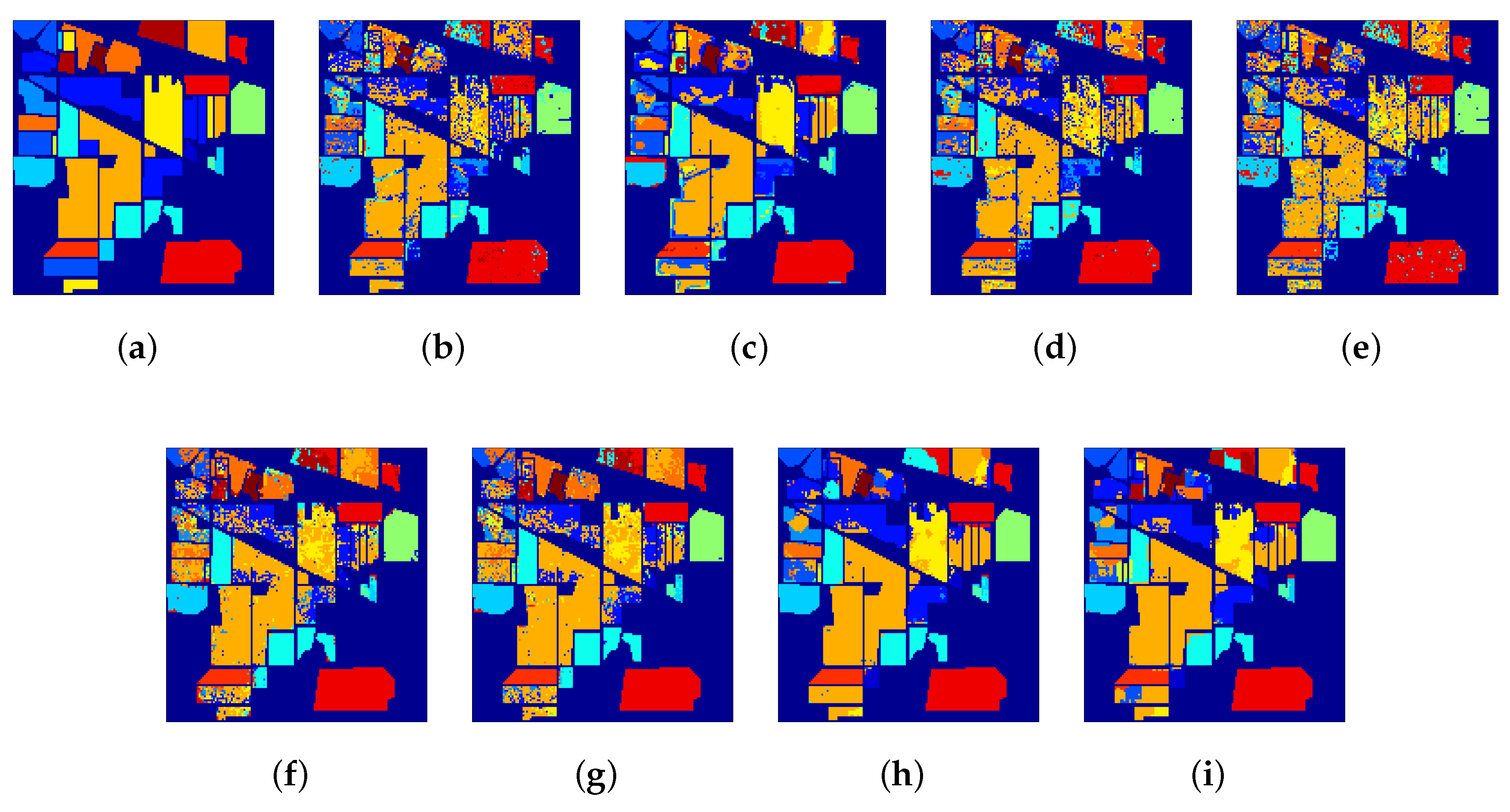
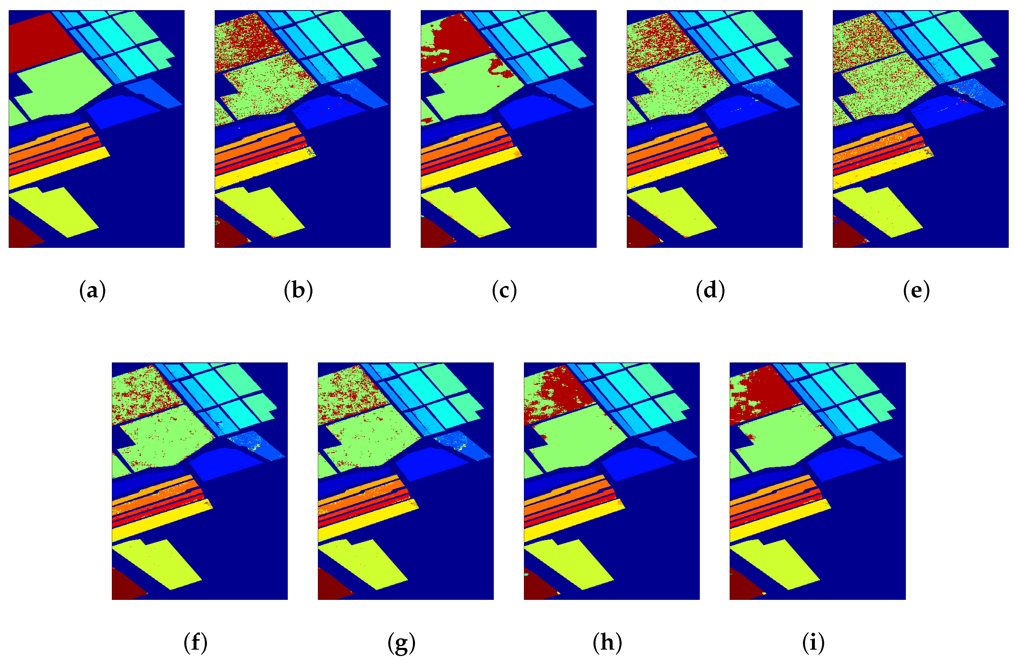
Figure 4 and Figure 5 show the classification maps obtained by different algorithms. The spectral-based methods (i.e., SVM, SRC, and OMP) generate very bad results with too much “salt & pepper” noise because they only use the spectral information without using spatial neighborhood information. Spatial–spectral-based methods greatly improve the classification performance. Compared with KJSR, our SPKJSR shows relatively better results. In particular, with the Salinas data set, traditional sparse-based methods, such as SRC, OMP, JSR, and WJSR, almost wrongly classify Class No. 15 “Vineyard untrained” as Class No. 8 “Grape untrained”. These two classes are spatially adjacent, so their spectral characteristics are very similar. It is very difficult to classify these spectrally similar classes. This notwithstanding, our SPKJSR can still discriminate the subtle differences between these two classes and provides desirable results.
The computational times for different methods when reaching their optimal classification performances are reported in Table 6. Because sparse models need to make predictions for each test sample separately, they are usually more time-consuming. As an iterative algorithm, the proposed SPKJSR is relatively slower than JSR and KJSR.
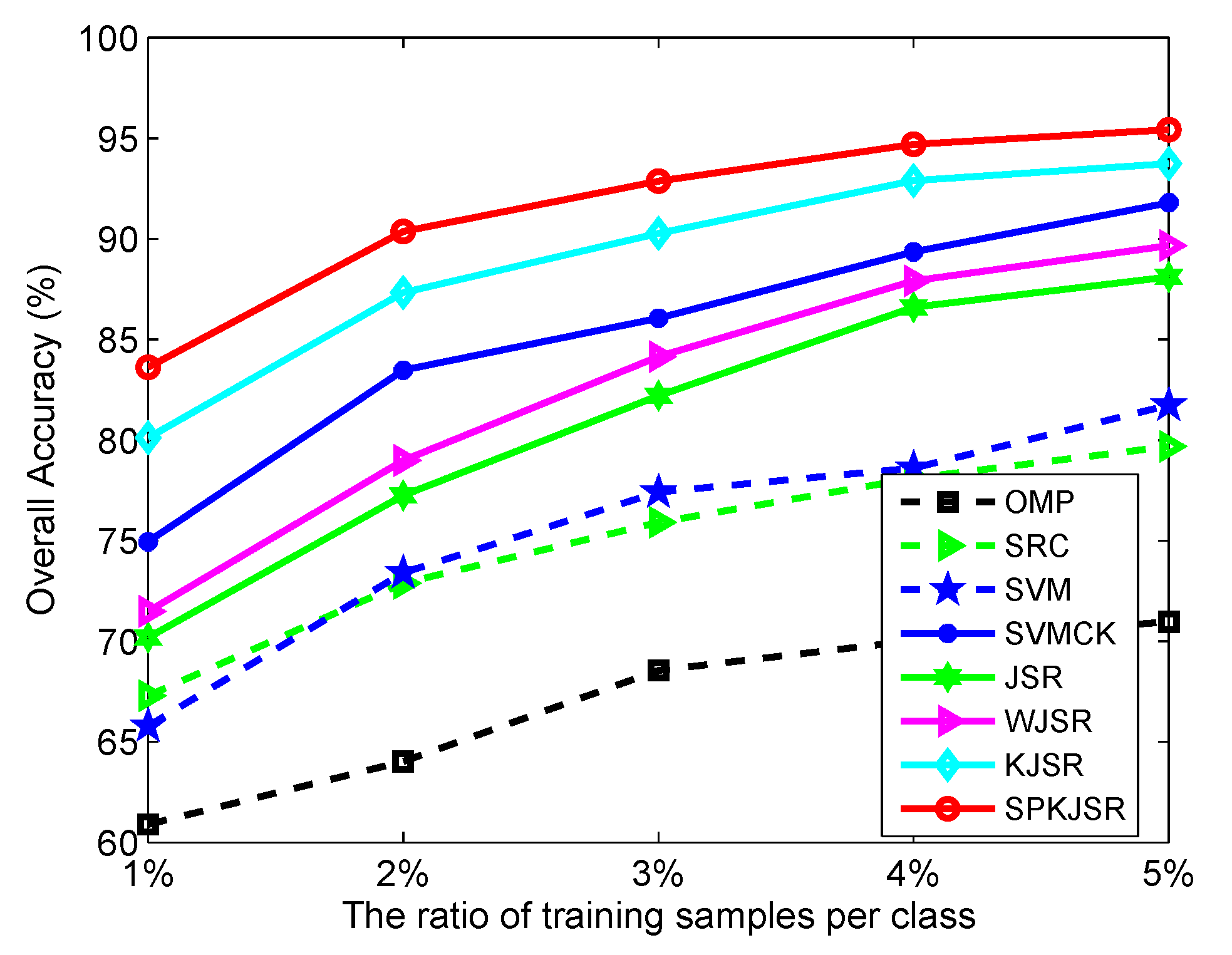
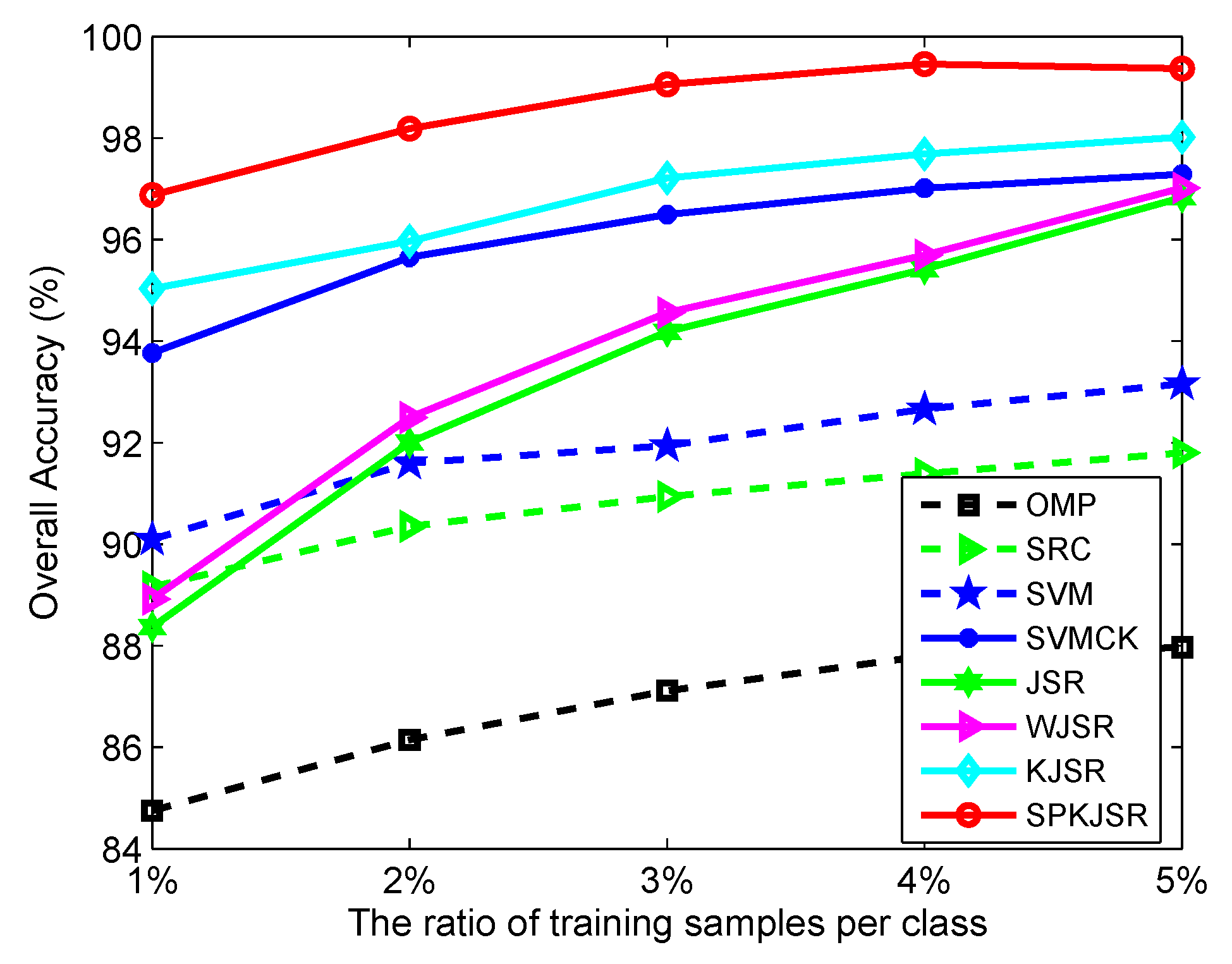
In the previous experiments, we have evaluated the effectiveness of our proposed SPKJSR in the case of small sample sizes (i.e., 1% of samples per class for training). Here, we further show the results for a large number of training samples and analyze the effect of the number of training samples. For this purpose, we draw 1%, 2%, 3%, 4%, and 5% of labeled samples from each class to form the training set and then evaluate the performance of different algorithms on the corresponding testing set. Figure 6 and Figure 7 show the OA of different methods versus the ratio of training samples per class for the Indian Pines and Salinas data sets, respectively. It can clearly be seen that SPKJSR provides consistently better results than the other algorithms with different numbers of training samples. Compared with the original linear JSR method, kernel-based KJSR and SPKJSR show a great performance improvement, which demonstrates the effectiveness of the kernel method for describing the intrinsic nonlinear relations of hyperspectral data.
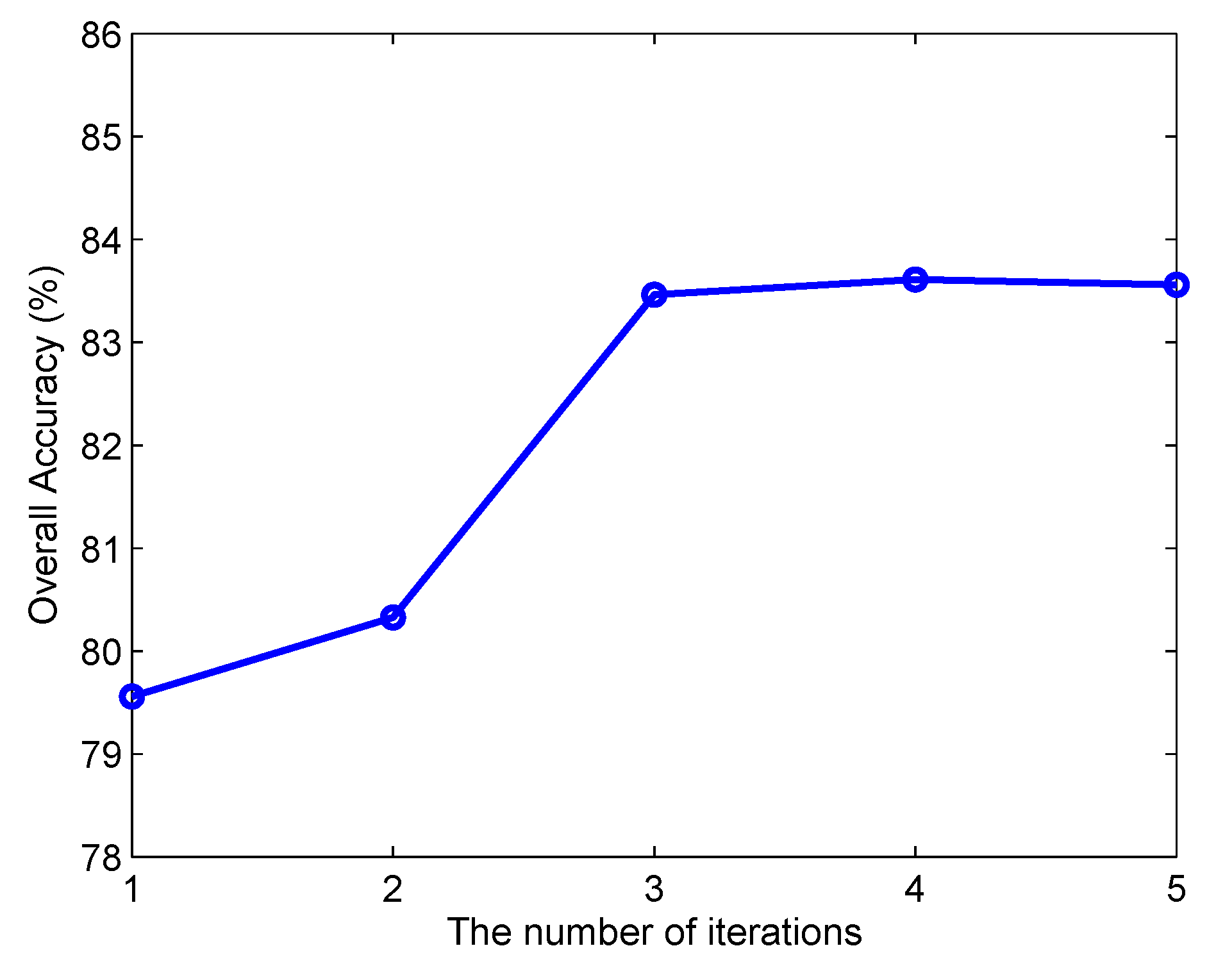
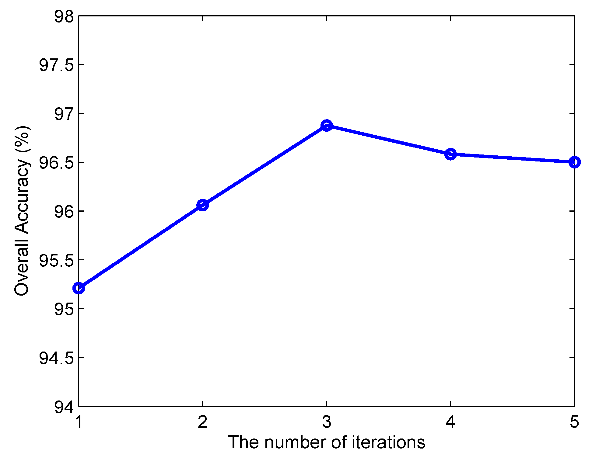
As shown in Algorithm 2, SPKJSR employs an alternative iterative strategy to update the sparsity coefficient matrix and weight matrix, so it is an iterative algorithm. Now, we investigate the effect of the number of iterations. Figure 8 and Figure 9 show the classification OA versus the number of iterations on the Indian Pines and Salinas data sets, respectively. It can be seen that the proposed algorithm achieves relatively better performance after 3 iterations.
4. Discussions
From the previous results in Table 3 and Table 4, we can see that KJSR dramatically improves the original JSR. This demonstrates that kernel representation is effective for modeling the nonlinear relation between hyperspectral pixels [24]. In addition, the improvement of WJSR over JSR demonstrates that pixels in a spatial neighborhood have differences, and the weighted strategy can alleviate the negative effect of noisy or inhomogeneous pixels in the neighborhood [10]. Due to the presence of noisy neighboring pixels, directly performing kernel representation on these noisy pixels may not be robust. Our proposed SPKJSR model provides a robust kernel representation to improve the robustness of the joint representation of neighboring pixels in the feature space.
Although many existing JSR methods have tried to eliminate noisy or inhomogeneous pixels in the spatial neighborhood in a preprocessing step by means of image segmentation techniques [12,13,14], they usually suffer from an inaccurate identification of inhomogeneous neighboring pixels. The identification of pixels is based on spectral similarity, which is usually inaccurate due to the spectral variation of spatially adjacent pixels. Rather than deleting inhomogeneous pixels in advance, defining a robust metric has proven to be effective for suppressing the effect of inhomogeneous pixels on the JSR model [15,17,18]. Some robust metrics, such as correntropy-based metrics [15] and maximum likelihood estimation-based metrics [18,36], are used. This notwithstanding, in the feature space, there is a lack of robust metrics on kernel representation for the KJSR model. To the best of our knowledge, this paper is the first to provide a robust kernel representation for the KJSR model.
5. Conclusions
We have proposed a self-paced kernel joint sparse representation (SPKJSR) model for hyperspectral image classification. The proposed SPKJSR mainly improves the feature neighboring pixel representation in the traditional kernel joint sparse representation (KJSR) model. By introducing a self-paced learning strategy, the proposed SPKJSR simultaneously optimizes the sparsity coefficient matrix and weight matrix for feature neighboring pixels in a regularized KJSR framework. The optimized weight can indicate the difficulty of neighboring pixels. The inhomogeneous or noisy neighboring pixels are assigned a small weight or 0 weight and hence produce very limited effects on the joint sparse representation. Thus, SPKJSR is much more robust and accurate than the traditional kernel joint sparse representation method. To validate the effectiveness of the proposed method, we have performed experiments on two benchmark hyperspectral data sets: Indian Pines and Salinas. Experimental results have shown that the proposed SPKJSR provides consistently better results than other existing joint sparse representation methods. In particular, when only 1% of samples per class are use for training, SPKJSR improves the overall accuracy of KJSR by about 3.5% on the Indian Pines data set and 1.8% on the Salinas data set. In the future, we will consider using different kinds of kernels for the KJSR model, such as spatial–spectral-based kernels and Log-Euclidean kernels.
Author Contributions
Conceptualization, S.H., J.P., Y.F., and L.L.; Methodology, S.H., J.P., Y.F., and L.L.; Software, S.H. and J.P.; Validation, J.P. and Y.F.; Formal analysis, S.H., J.P., and Y.F.; Investigation, S.H., J.P., and L.L.; Resources, J.P. and L.L.; Writing—original draft preparation, S.H. and J.P.; Writing—review and editing, S.H., J.P., Y.F., and L.L.; Supervision, J.P., Y.F., and L.L.
Funding
This research was funded by the National Natural Science Foundation of China under Grant Nos. 61871177 and 11771130.
Acknowledgments
The authors would like to thank D. Landgrebe for providing the Indian Pines data set and J. Anthony Gualtieri for providing the Salinas data set.
Conflicts of Interest
The authors declare no conflict of interest.
Abbreviations
The following abbreviations are used in this manuscript:
| HSI | Hyperspectral image |
| JSR | Joint sparse representation |
| KJSR | Kernel joint sparse representation |
| SPL | Self-paced learning |
| SPKJSR | Self-paced kernel joint sparse representation |
| SOMP | Simultaneous orthogonal matching pursuit |
| KSOMP | Kernel simultaneous orthogonal matching pursuit |
References
- Bioucas-Dias, J.M.; Plaza, A.; Camps-Valls, G.; Scheunders, P.; Nasrabadi, N.; Chanussot, J. Hyperspectral remote sensing data analysis and future challenges. IEEE Geosci. Remote Sens. Mag. 2013, 1, 6–36. [Google Scholar] [CrossRef]
- Fauvel, M.; Tarabalka, Y.; Benediktsson, J.A.; Chanussot, J.; Tilton, J.C. Advances in spectral-spatial classification of hyperspectral images. Proc. IEEE 2013, 101, 652–675. [Google Scholar] [CrossRef]
- Mallinis, G.; Galidaki, G.; Gitas, I. A comparative analysis of EO-1 Hyperion, Quickbird and Landsat TM imagery for fuel type mapping of a typical mediterranean landscape. Remote Sens. 2014, 6, 1684–1704. [Google Scholar] [CrossRef]
- Zhou, Y.; Peng, J.; Chen, C.L.P. Dimension reduction using spatial and spectral regularized local discriminant embedding for hyperspectral image classification. IEEE Trans. Geosci. Remote Sens. 2015, 53, 1082–1095. [Google Scholar] [CrossRef]
- He, L.; Li, J.; Liu, C.; Li, S. Recent advances on spectral-spatial hyperspectral image classification: An overview and new guidelines. IEEE Trans. Geosci. Remote Sens. 2018, 56, 1579–1597. [Google Scholar] [CrossRef]
- Camps-Valls, G.; Gomez-Chova, L.; Munoz-Mare, J.; Vila-Frances, J.; Calpe-Maravilla, J. Composite kernels for hyperspectral image classification. IEEE Geosci. Remote Sens. Lett. 2006, 3, 93–97. [Google Scholar] [CrossRef]
- Zhou, Y.; Peng, J.; Chen, C.L.P. Extreme learning machine with composite kernels for hyperspectral image classification. IEEE J. Sel. Top. Appl. Earth Obs. Remote Sens. 2015, 8, 2351–2360. [Google Scholar] [CrossRef]
- Peng, J.; Zhou, Y.; Chen, C.L.P. Region-kernel-based support vector machines for hyperspectral image classification. IEEE Trans. Geosci. Remote Sens. 2015, 53, 4810–4824. [Google Scholar] [CrossRef]
- Chen, Y.; Nasrabadi, N.; Tran, T. Hyperspectral image classification using dictionary-based sparse representation. IEEE Trans. Geosci. Remote Sens. 2011, 49, 3973–3985. [Google Scholar] [CrossRef]
- Zhang, H.; Li, J.; Huang, Y.; Zhang, L. A nonlocal weighted joint sparse representation classification method for hyperspectral imagery. IEEE J. Sel. Top. Appl. Earth Obs. Remote Sens. 2014, 7, 2057–2066. [Google Scholar]
- Chen, C.; Chen, N.; Peng, J. Nearest regularized joint sparse representation for hyperspectral image classification. IEEE Geosci. Remote Sens. Lett. 2016, 13, 424–428. [Google Scholar] [CrossRef]
- Zou, J.; Li, W.; Huang, X.; Du, Q. Classification of hyperspectral urban data using adaptive simultaneous orthogonal matching pursuit. J. Appl. Remote Sens. 2014, 8, 085099. [Google Scholar] [CrossRef]
- Fang, L.; Li, S.; Kang, X.; Benediktsson, J.A. Spectral-spatial classification of hyperspectral images with a superpixel-based discriminative sparse model. IEEE Trans. Geosci. Remote Sens. 2015, 53, 4186–4201. [Google Scholar] [CrossRef]
- Fu, W.; Li, S.; Fang, L.; Benediktsson, J.A. Hyperspectral image classification via shapeadaptive joint sparse representation. IEEE J. Sel. Top. Appl. Earth Obs. Remote Sens. 2016, 9, 556–567. [Google Scholar] [CrossRef]
- Peng, J.; Du, Q. Robust joint sparse representation based on maximum correntropy criterion for hyperspectral image classification. IEEE Trans. Geosci. Remote Sens. 2017, 55, 7152–7164. [Google Scholar] [CrossRef]
- Wu, C.; Du, B.; Zhang, L. Hyperspectral anomalous change detection based on joint sparse representation. ISPRS J. Photogramm. Remote Sens. 2018, 146, 137–150. [Google Scholar] [CrossRef]
- Peng, J.; Sun, W.; Du, Q. Self-paced joint sparse representation for the classification of hyperspectral images. IEEE Trans. Geosci. Remote Sens. 2019, 57, 1183–1194. [Google Scholar] [CrossRef]
- Peng, J.; Li, L.; Tang, Y. Maximum likelihood estimation based joint sparse representation for the classification of hyperspectral remote sensing images. IEEE Trans. Neural Netw. Learn. Syst. 2018. [Google Scholar] [CrossRef]
- Hu, S.; Xu, C.; Peng, J.; Xu, Y.; Tian, L. Weighted kernel joint sparse representation for hyperspectral image classification. IET Image Process. 2019, 13, 254–260. [Google Scholar] [CrossRef]
- Camps-Valls, G.; Bruzzone, L. Kernel-based methods for hyperspectral image classification. IEEE Trans. Geosci. Remote Sens. 2005, 43, 1351–1362. [Google Scholar] [CrossRef]
- Peng, J.; Chen, H.; Zhou, Y.; Li, L. Ideal regularized composite kernel for hyperspectral image classification. IEEE J. Sel. Top. Appl. Earth Obs. Remote Sens. 2017, 10, 1563–1574. [Google Scholar] [CrossRef]
- Heylen, R.; Parente, M.; Gader, P. A review of nonlinear hyperspectral unmixing methods. IEEE J. Sel. Top. Appl. Earth Obs. Remote Sens. 2014, 7, 1844–1868. [Google Scholar] [CrossRef]
- Han, H.; Goodenough, D.G. Investigation of Nonlinearity in Hyperspectral Imagery Using Surrogate Data Methods. IEEE Trans. Geosci. Remote Sens. 2008, 46, 2840–2847. [Google Scholar] [CrossRef]
- Chen, Y.; Nasrabadi, N.; Tran, T. Hyperspectral image classification via kernel sparse representation. IEEE Trans. Geosci. Remote Sens. 2013, 51, 217–231. [Google Scholar] [CrossRef]
- Wang, J.; Jiao, L.; Liu, H.; Yang, S.; Liu, F. Hyperspectral image classification by spatial-spectral derivative-aided kernel joint sparse representation. IEEE J. Sel. Top. Appl. Earth Obs. Remote Sens. 2015, 8, 2485–2500. [Google Scholar] [CrossRef]
- Zhang, E.; Zhang, X.; Jiao, L.; Liu, H.; Wang, S.; Hou, B. Weighted multifeature hyperspectral image classification via kernel joint sparse representation. Neurocomputing 2016, 178, 71–86. [Google Scholar] [CrossRef]
- Bengio, Y.; Louradour, J.; Collobert, R.; Weston, J. Curriculum learning. In International Conference on Machine Learning (ICML); ACM: New York, NY, USA, 2009; pp. 41–48. [Google Scholar]
- Jiang, Y.; Meng, D.; Zhao, Q.; Shan, S.; Hauptmann, A. Self-paced curriculum learning. In Proceedings of the Twenty-Ninth AAAI Conference on Artificial Intelligence (AAAI), Austin, TX, USA, 25–30 January 2015; pp. 2694–2700. [Google Scholar]
- Meng, D.; Zhao, Q.; Jiang, L. A theoretical understanding of self-paced learning. Inf. Sci. 2017, 414, 319–328. [Google Scholar] [CrossRef]
- Tang, Y.; Wang, X.; Harrison, A.P.; Lu, L.; Xiao, J.; Summers, R.M. Attention-guided curriculum learning for weakly supervised classification and localization of thoracic diseases on chest radiographs. In International Workshop on Machine Learning in Medical Imaging (MLMI); Springer: Cham, Switzerland, 2018; pp. 249–258. [Google Scholar]
- Wu, Y.; Tian, Y. Training agent for first-person shooter game with actor-critic curriculum learning. In Proceedings of the International Conference on Learning Representations (ICLR), Toulon, France, 24–26 April 2017. [Google Scholar]
- Wright, J.; Yang, A.Y.; Ganesh, A.; Sastry, S.; Ma, Y. Robust face recognition via sparse representation. IEEE Trans. Pattern Anal. Mach. Intell. 2009, 31, 210–227. [Google Scholar] [CrossRef] [PubMed]
- Tropp, J.A.; Gilbert, A.C.; Strauss, M.J. Algorithms for simultaneous sparse approximation. Part I: Greedy pursuit. Signal Process. 2006, 86, 572–588. [Google Scholar] [CrossRef]
- Foody, G.M. Thematic map comparison: Evaluating the statistical significance of differences in classification accuracy. Photogramm. Eng. Remote Sens. 2004, 70, 627–633. [Google Scholar] [CrossRef]
- Fauvel, M.; Benediktsson, J.A.; Chanussot, J.; Sveinsson, J.R. Spectral and spatial classification of hyperspectral data using SVMs and morphological profiles. IEEE Trans. Geosci. Remote Sens. 2008, 46, 3804–3814. [Google Scholar] [CrossRef]
- Yang, M.; Zhang, L.; Shiu, S.; Zhang, D. Robust Kernel Representation With Statistical Local Features for Face Recognition. IEEE Trans. Neural Netw. Learn. Syst. 2013, 24, 900–912. [Google Scholar] [CrossRef]
Figure 1.
Sketches of sparse representation and joint sparse representation. (a) Sparse Representation; (b) Joint Sparse Representation.
Figure 1.
Sketches of sparse representation and joint sparse representation. (a) Sparse Representation; (b) Joint Sparse Representation.

Figure 2.
Indian Pines data set. (a) RGB composite image; (b) ground-truth map.

Figure 3.
Salinas data set. (a) RGB composite image; (b) ground-truth map.

Figure 4.
Indian Pines: (a) Ground-truth map; classification maps obtained by (b) SVM (65.78%), (c) SVMCK (74.94%); (d) SRC (67.28%); (e) OMP (60.89%); (f) JSR (70.18%); (g) WJSR (71.48%); (h) KJSR (80.11%); and (i) SPKJSR (83.61%).
Figure 4.
Indian Pines: (a) Ground-truth map; classification maps obtained by (b) SVM (65.78%), (c) SVMCK (74.94%); (d) SRC (67.28%); (e) OMP (60.89%); (f) JSR (70.18%); (g) WJSR (71.48%); (h) KJSR (80.11%); and (i) SPKJSR (83.61%).

Figure 5.
Salinas: (a) Ground-truth map; classification maps obtained by (b) SVM (90.09%); (c) SVMCK (93.77%); (d) SRC (89.16%); (e) OMP (84.75%); (f) JSR (88.37%); (g) WJSR (88.92%); (h) KJSR (95.03%); and (i) SPKJSR (96.88%).
Figure 5.
Salinas: (a) Ground-truth map; classification maps obtained by (b) SVM (90.09%); (c) SVMCK (93.77%); (d) SRC (89.16%); (e) OMP (84.75%); (f) JSR (88.37%); (g) WJSR (88.92%); (h) KJSR (95.03%); and (i) SPKJSR (96.88%).

Figure 6.
OA versus the number of training samples on Indian Pines.

Figure 7.
OA versus the number of training samples on Salinas.

Figure 8.
OA versus the number of iterations on Indian Pines.

Figure 9.
OA versus the number of iterations on Salinas.


Table 1.
The number of training and testing samples for each class in the Indian Pines data set (only 1% of labeled samples per class for training, with a total of 115 training samples and 10,251 testing samples).
Table 1.
The number of training and testing samples for each class in the Indian Pines data set (only 1% of labeled samples per class for training, with a total of 115 training samples and 10,251 testing samples).
| No | Class | #Train | #Test | No | Class | #Train | #Test |
|---|---|---|---|---|---|---|---|
| 1 | Alfalfa | 3 | 51 | 9 | Oats | 3 | 17 |
| 2 | Corn-notill | 14 | 1420 | 10 | Soybean-notill | 10 | 958 |
| 3 | Corn-mintill | 8 | 826 | 11 | Soybean-mintill | 25 | 2443 |
| 4 | Corn | 3 | 231 | 12 | Soybean-clean | 6 | 608 |
| 5 | Grass-pasture | 5 | 492 | 13 | Wheat | 3 | 209 |
| 6 | Grass-trees | 7 | 740 | 14 | Woods | 13 | 1281 |
| 7 | Grass-pasture-mowed | 3 | 23 | 15 | Buildings-Grass-Trees-Drives | 4 | 376 |
| 8 | Hay-windrowed | 5 | 484 | 16 | Stone-Steel-Towers | 3 | 92 |
Table 2.
The number of training and testing samples for each class in the Salinas data set (only 1% of labeled samples per class for training, with a total of 543 training samples and 53,586 testing samples).
Table 2.
The number of training and testing samples for each class in the Salinas data set (only 1% of labeled samples per class for training, with a total of 543 training samples and 53,586 testing samples).
| No | Class | #Train | #Test | No | Class | #Train | #Test |
|---|---|---|---|---|---|---|---|
| 1 | Weeds1 | 20 | 1989 | 9 | Soil | 62 | 6141 |
| 2 | Weeds2 | 37 | 3689 | 10 | Corn | 33 | 3245 |
| 3 | Fallow | 20 | 1956 | 11 | Lettuce 4wk | 11 | 1057 |
| 4 | Fallow plow | 14 | 1380 | 12 | Lettuce 5wk | 19 | 1908 |
| 5 | Fallow smooth | 27 | 2651 | 13 | Lettuce 6wk | 9 | 907 |
| 6 | Stubble | 40 | 3919 | 14 | Lettuce 7wk | 11 | 1059 |
| 7 | Celery | 36 | 3543 | 15 | Vineyard untrained | 73 | 7195 |
| 8 | Grapes untrained | 113 | 11158 | 16 | Vineyard trellis | 18 | 1789 |
Table 3.
Overall, average, and individual class accuracies and statistics in the form of mean ± standard deviation for the Indian Pines data set. The best results are highlighted in bold typeface.
Table 3.
Overall, average, and individual class accuracies and statistics in the form of mean ± standard deviation for the Indian Pines data set. The best results are highlighted in bold typeface.
| Class | SVM | SVMCK | SRC | OMP | JSR | WJSR | KJSR | SPKJSR |
|---|---|---|---|---|---|---|---|---|
| 1 | 66.01 ± 5.99 | 66.01 ± 17.7 | 66.01 ± 8.16 | 58.82 ± 5.19 | 79.08 ± 5.99 | 77.12 ± 22.0 | 88.89 ± 4.93 | 96.73 ± 4.08 |
| 2 | 59.27 ± 1.89 | 79.13 ± 9.15 | 52.37 ± 5.55 | 44.51 ± 7.65 | 55.73 ± 2.11 | 58.10 ± 6.09 | 74.79 ± 6.20 | 79.53 ± 5.03 |
| 3 | 47.94 ± 2.00 | 69.49 ± 9.28 | 48.38 ± 7.04 | 35.27 ± 1.46 | 41.49 ± 20.3 | 41.81 ± 18.0 | 63.64 ± 8.78 | 67.96 ± 8.35 |
| 4 | 46.32 ± 6.80 | 57.72 ± 26.4 | 50.07 ± 3.28 | 33.77 ± 6.75 | 36.22 ± 1.64 | 34.34 ± 3.19 | 73.30 ± 11.2 | 83.41 ± 6.30 |
| 5 | 82.45 ± 6.67 | 62.60 ± 10.0 | 65.51 ± 10.4 | 73.37 ± 7.22 | 73.10 ± 7.07 | 75.34 ± 8.98 | 79.06 ± 7.27 | 79.05 ± 5.38 |
| 6 | 89.50 ± 4.17 | 89.10 ± 5.66 | 93.02 ± 3.69 | 89.05 ± 5.63 | 98.11 ± 0.95 | 98.65 ± 0.62 | 98.38 ± 0.62 | 90.50 ± 4.03 |
| 7 | 95.65 ± 4.35 | 92.75 ± 6.64 | 85.51 ± 5.02 | 85.51 ± 2.51 | 71.01 ± 13.3 | 88.41 ± 10.0 | 91.30 ± 11.5 | 100.0 ± 0 |
| 8 | 89.26 ± 3.96 | 83.47 ± 12.0 | 94.15 ± 1.47 | 92.29 ± 2.07 | 97.86 ± 1.14 | 99.66 ± 0.12 | 99.93 ± 0.12 | 99.93 ± 0.12 |
| 9 | 98.04 ± 3.40 | 96.08 ± 3.40 | 96.08 ± 6.79 | 74.51 ± 18.9 | 45.10 ± 8.98 | 74.51 ± 23.8 | 72.55 ± 3.40 | 94.12 ± 5.88 |
| 10 | 50.45 ± 21.0 | 65.27 ± 11.6 | 54.07 ± 10.9 | 47.88 ± 10.5 | 31.94 ± 5.53 | 31.91 ± 3.55 | 75.16 ± 12.3 | 79.71 ± 12.7 |
| 11 | 67.18 ± 8.04 | 73.77 ± 2.71 | 71.73 ± 4.37 | 62.44 ± 6.98 | 80.91 ± 3.73 | 83.63 ± 3.33 | 86.64 ± 4.75 | 89.78 ± 2.72 |
| 12 | 35.85 ± 4.94 | 59.37 ± 14.1 | 45.34 ± 14.3 | 38.32 ± 6.77 | 56.36 ± 15.5 | 57.84 ± 14.0 | 51.10 ± 16.7 | 61.51 ± 9.14 |
| 13 | 96.97 ± 1.93 | 81.50 ± 18.0 | 99.20 ± 0.28 | 96.81 ± 2.64 | 98.40 ± 1.38 | 99.52 ± 0.83 | 99.84 ± 0.28 | 92.18 ± 3.44 |
| 14 | 86.78 ± 4.11 | 92.53 ± 4.69 | 94.87 ± 1.65 | 89.69 ± 2.38 | 98.83 ± 0.79 | 99.53 ± 0.47 | 99.79 ± 0.16 | 99.32 ± 1.03 |
| 15 | 23.14 ± 8.98 | 45.92 ± 10.8 | 13.83 ± 4.18 | 16.58 ± 4.85 | 44.50 ± 16.6 | 39.36 ± 20.1 | 16.49 ± 15.1 | 49.56 ± 5.49 |
| 16 | 89.13 ± 4.74 | 100.0 ± 0 | 88.77 ± 5.99 | 88.04 ± 6.05 | 96.01 ± 1.26 | 98.91 ± 1.09 | 86.59 ± 3.32 | 81.16 ± 7.63 |
| OA | 65.78 ± 1.56 | 74.94 ± 3.55 | 67.28 ± 1.35 | 60.89 ± 1.47 | 70.18 ± 0.24 | 71.48 ± 0.64 | 80.11 ± 1.86 | 83.61 ± 1.48 |
| AA | 70.25 ± 24.0 | 75.92 ± 15.8 | 69.93 ± 24.6 | 64.18 ± 25.5 | 69.04 ± 24.7 | 72.41 ± 25.2 | 78.59 ± 21.7 | 84.03 ± 14.5 |
| 61.02 ± 1.90 | 71.49 ± 4.05 | 62.65 ± 1.82 | 55.44 ± 1.83 | 65.60 ± 0.37 | 66.98 ± 0.86 | 77.13 ± 2.32 | 81.19 ± 1.87 |
Table 4.
Overall, average, and individual class accuracies and statistics in the form of mean ± standard deviation for the Salinas data set. The best results are highlighted in bold typeface.
Table 4.
Overall, average, and individual class accuracies and statistics in the form of mean ± standard deviation for the Salinas data set. The best results are highlighted in bold typeface.
| Class | SVM | SVMCK | SRC | OMP | JSR | WJSR | KJSR | SPKJSR |
|---|---|---|---|---|---|---|---|---|
| 1 | 99.06 ± 0.45 | 96.61 ± 5.82 | 99.41 ± 0.48 | 99.14 ± 0.30 | 100.0 ± 0 | 100.0 ± 0 | 100.0 ± 0 | 100.0 ± 0 |
| 2 | 98.48 ± 0.33 | 99.86 ± 0.18 | 98.74 ± 0.76 | 98.24 ± 1.62 | 99.96 ± 0.04 | 99.95 ± 0.05 | 100.0 ± 0 | 100.0 ± 0 |
| 3 | 94.24 ± 4.49 | 98.91 ± 1.58 | 93.39 ± 1.39 | 88.05 ± 3.04 | 92.09 ± 3.16 | 92.04 ± 2.98 | 99.97 ± 0.06 | 100.0 ± 0 |
| 4 | 98.21 ± 1.22 | 94.86 ± 1.62 | 98.86 ± 0.55 | 94.23 ± 4.47 | 96.45 ± 3.01 | 96.47 ± 3.10 | 99.08 ± 1.41 | 96.52 ± 2.02 |
| 5 | 97.14 ± 1.36 | 97.51 ± 1.60 | 98.16 ± 0.83 | 91.56 ± 0.58 | 88.32 ± 2.12 | 93.19 ± 2.67 | 99.71 ± 0.30 | 99.56 ± 0.08 |
| 6 | 99.56 ± 0.21 | 98.94 ± 1.72 | 99.72 ± 0.17 | 99.82 ± 0.03 | 99.95 ± 0.07 | 99.96 ± 0.01 | 100.0 ± 0 | 99.91 ± 0.05 |
| 7 | 99.27 ± 0.10 | 99.08 ± 0.47 | 99.28 ± 0.20 | 99.63 ± 0.12 | 99.89 ± 0.15 | 99.91 ± 0.03 | 100.0 ± 0 | 100.0 ± 0 |
| 8 | 86.28 ± 4.77 | 93.07 ± 0.72 | 85.07 ± 1.44 | 78.08 ± 1.44 | 94.54 ± 0.65 | 94.89 ± 0.82 | 96.97 ± 1.54 | 97.66 ± 0.84 |
| 9 | 97.81 ± 0.99 | 97.33 ± 2.67 | 98.01 ± 0.36 | 97.65 ± 0.67 | 99.31 ± 0.63 | 99.26 ± 0.68 | 100.0 ± 0 | 100.0 ± 0 |
| 10 | 87.98 ± 8.27 | 93.71 ± 1.63 | 90.92 ± 2.82 | 88.02 ± 0.96 | 93.97 ± 1.32 | 94.96 ± 1.98 | 96.48 ± 1.80 | 97.41 ± 1.74 |
| 11 | 92.21 ± 4.90 | 88.46 ± 9.11 | 93.38 ± 4.99 | 92.75 ± 4.98 | 94.04 ± 3.45 | 95.05 ± 2.79 | 99.27 ± 0.55 | 99.84 ± 0.05 |
| 12 | 99.86 ± 0.24 | 99.86 ± 0.20 | 99.95 ± 0 | 86.48 ± 4.06 | 84.26 ± 10.7 | 85.17 ± 10.8 | 100.0 ± 0 | 99.84 ± 0.10 |
| 13 | 97.43 ± 0.23 | 98.53 ± 1.40 | 97.57 ± 0.22 | 89.12 ± 2.61 | 78.61 ± 3.06 | 88.31 ± 3.25 | 98.97 ± 0.50 | 99.34 ± 0.22 |
| 14 | 92.63 ± 1.18 | 96.51 ± 0.96 | 92.79 ± 1.13 | 90.97 ± 0.85 | 95.62 ± 1.56 | 94.65 ± 0.73 | 99.40 ± 0.38 | 98.62 ± 1.66 |
| 15 | 62.53 ± 4.31 | 76.72 ± 3.94 | 54.91 ± 2.18 | 44.80 ± 2.88 | 40.95 ± 13.2 | 40.81 ± 13.1 | 70.28 ± 3.08 | 83.00 ± 1.70 |
| 16 | 97.82 ± 1.12 | 97.59 ± 2.17 | 98.56 ± 0.43 | 97.06 ± 1.80 | 99.29 ± 0.34 | 99.39 ± 0.51 | 98.58 ± 0.80 | 99.03 ± 0.76 |
| OA | 90.09 ± 1.08 | 93.77 ± 0.40 | 89.16 ± 0.33 | 84.75 ± 0.52 | 88.37 ± 2.05 | 88.92 ± 1.99 | 95.03 ± 0.28 | 96.88 ± 0.26 |
| AA | 93.78 ± 9.30 | 95.47 ± 5.83 | 93.67 ± 11.1 | 89.73 ± 13.4 | 91.08 ± 14.7 | 92.12 ± 14.4 | 97.42 ± 7.32 | 98.17 ± 4.18 |
| 88.95 ± 1.21 | 93.05 ± 0.45 | 87.90 ± 0.38 | 82.98 ± 0.59 | 86.97 ± 2.32 | 87.58 ± 2.24 | 94.46 ± 0.31 | 96.52 ± 0.29 |
Table 5.
Z values of McNemar’s test between the proposed SPKJSR and other methods.
| SVM | SVMCK | SRC | OMP | JSR | WJSR | KJSR | |
|---|---|---|---|---|---|---|---|
| Indian Pines | −33.18 | −15.56 | −32.69 | −40.33 | −23.60 | −21.59 | −11.04 |
| Salinas | −54.52 | −27.20 | −57.54 | −76.39 | −68.47 | −65.61 | −25.53 |
Table 6.
The running time of different methods.
| SVM | SVMCK | SRC | OMP | JSR | WJSR | KJSR | SPKJSR | |
|---|---|---|---|---|---|---|---|---|
| Indian Pines | 0.3 | 2.2 | 21 | 20 | 152 | 169 | 75 | 243 |
| Salinas | 1.9 | 17 | 198 | 133 | 1380 | 1599 | 998 | 3061 |
© 2019 by the authors. Licensee MDPI, Basel, Switzerland. This article is an open access article distributed under the terms and conditions of the Creative Commons Attribution (CC BY) license (http://creativecommons.org/licenses/by/4.0/).
Share and Cite
MDPI and ACS Style
Hu, S.; Peng, J.; Fu, Y.; Li, L. Kernel Joint Sparse Representation Based on Self-Paced Learning for Hyperspectral Image Classification. Remote Sens. 2019, 11, 1114. https://0-doi-org.brum.beds.ac.uk/10.3390/rs11091114
AMA Style
Hu S, Peng J, Fu Y, Li L. Kernel Joint Sparse Representation Based on Self-Paced Learning for Hyperspectral Image Classification. Remote Sensing. 2019; 11(9):1114. https://0-doi-org.brum.beds.ac.uk/10.3390/rs11091114
Chicago/Turabian StyleHu, Sixiu, Jiangtao Peng, Yingxiong Fu, and Luoqing Li. 2019. "Kernel Joint Sparse Representation Based on Self-Paced Learning for Hyperspectral Image Classification" Remote Sensing 11, no. 9: 1114. https://0-doi-org.brum.beds.ac.uk/10.3390/rs11091114
Note that from the first issue of 2016, this journal uses article numbers instead of page numbers. See further details here.