Deep Learning Based Fossil-Fuel Power Plant Monitoring in High Resolution Remote Sensing Images: A Comparative Study


1
Image Processing Center, School of Astronautics, Beihang University, Beijing 100191, China
2
Key Laboratory of Spacecraft Design Optimization and Dynamic Simulation Technologies, Ministry of Education, Beijing 100191, China
3
Beijing Key Laboratory of Digital Media, Beijing 100191, China
*
Author to whom correspondence should be addressed.
†
These authors contributed equally to this work.
Remote Sens. 2019, 11(9), 1117; https://0-doi-org.brum.beds.ac.uk/10.3390/rs11091117
Submission received: 21 April 2019
/
Revised: 29 April 2019
/
Accepted: 7 May 2019
/
Published: 10 May 2019
(This article belongs to the Special Issue Deep Learning Approaches for Urban Sensing Data Analytics)
Abstract
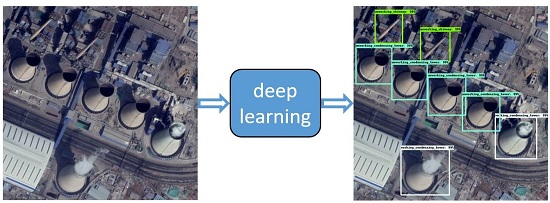
:The frequent hazy weather with air pollution in North China has aroused wide attention in the past few years. One of the most important pollution resource is the anthropogenic emission by fossil-fuel power plants. To relieve the pollution and assist urban environment monitoring, it is necessary to continuously monitor the working status of power plants. Satellite or airborne remote sensing provides high quality data for such tasks. In this paper, we design a power plant monitoring framework based on deep learning to automatically detect the power plants and determine their working status in high resolution remote sensing images (RSIs). To this end, we collected a dataset named BUAA-FFPP60 containing RSIs of over 60 fossil-fuel power plants in the Beijing-Tianjin-Hebei region in North China, which covers about 123 km of an urban area. We compared eight state-of-the-art deep learning models and comprehensively analyzed their performance on accuracy, speed, and hardware cost. Experimental results illustrate that our deep learning based framework can effectively detect the fossil-fuel power plants and determine their working status with mean average precision up to 0.8273, showing good potential for urban environment monitoring.

1. Introduction
Air pollution reaches a level pernicious to the health of the population and poses a threat to peoples’ daily life in the past few years in China. Especially in the Beijing-Tianjin-Hebei region, serious haze pollution frequently appears in winter. Haze event in North China is traditionally an atmospheric phenomenon where dust, smoke and other dry particles obscure the clarity of the sky [1]. However, due to the domestic and collective heating, more fine particulate matter (PM2.5) are discharged to the atmosphere as well as , , etc., leading the harmful haze pollution [2,3]. In other words, the burning of fossil-fuel, e.g., coal, is one of the most important pollution sources in the Beijing-Tianjin-Hebei region. Since fossil-fuel power plants usually burn a large amount of coal, monitoring the fossil-fuel power plants can help to control the anthropogenic emission and prevent air pollution. Without the difficulty of staffed daily monitoring, high resolution remote sensing provides an effective solution for such task by easily observing the running state of power plants from satellite or airborne imaging sensors. This application problem contains two aspects. One is to find the power plants in high resolution remote sensing images (RSIs), and the other is to check the working status of them. Nevertheless, manual interpretation of massive remote sensing data is time-consuming and inefficient. For example, a person may need several days to scan 1-m resolution optical RSIs to find the fossil-fuel power plants around Shijiazhuang, the capital city of Hebei province, yet the result may still be unreliable [4]. Therefore, it is better to solve this application problem automatically by recent artificial intelligence algorithms.
Recently, object detection in RSIs is a hotspot in remote sensing image understanding. Researchers focus on detecting various types of objects in RSIs, including aircrafts [5,6], ships [7,8,9], oil tanks [10,11,12], and so on. With the development of deep learning, such cutting edge technology has benefited remote sensing a lot [13], including object detection in RSIs. Deep learning based detection approaches usually outperform other traditional methods given large scale of labeled RSI data. There are also several publicly available datasets supporting such research, e.g., Northwestern Polytechnical University Very High Resolution remote sensing images (NWPU VHR-10) [14], LEarning, VIsion and Remote sensing laboratory (LEVIR) [15], and A Large-scale Dataset for Object DeTection in Aerial Images (DOTA) [16,17]. In terms of power plant monitoring, previously Yao et al. [4] studied one subproblem, i.e., power plant detection. Yao et al. [4] learned an integrated model for detecting chimney and condensing tower based on Faster Regions with Convolutional Neural Network (Faster R-CNN) [18]. Besides completing the mission of locating power plants, this method has three shortages. Firstly, images in the dataset provided in [4] have only two kinds of class labels, i.e., chimney and condensing tower. Thus, it cannot determine working status of the power plants. Secondly, it uses three fixed aspect ratios to generate proposals in Faster R-CNN. This may not fit the shape of chimneys and lead to relatively low accuracy. Lastly, no comparison was made to show whether Faster R-CNN can achieve better detection accuracy, shorter running time and less memory cost than other deep learning models.
Focus on the specific application problem of power plant monitoring, we follow Yao et al. [4] to collect a more comprehensive dataset that contains not only locations and class labels but also working status labels. We call this dataset BUAA-FFPP60, meaning that it contains RSIs of over 60 fossil-fuel power plants (FFPP) collected by researchers from Beihang University (BUAA). We design a power plant monitoring framework based on deep learning to automatically detect the power plants and determine their working status, giving complete solution for power plant monitoring. To find the most suitable deep learning model, we compared eight state-of-the-art deep learning models and comprehensively analyzed their performance on accuracy, speed, and hardware cost. Our framework and BUAA-FFPP60 dataset are publicly available from the corresponding author upon request or via the author’s website (https://github.com/SPDQ/Power-Plant-Detection-in-RSI, or https://haopzhang.github.io/), which could facilitate researchers to achieve urban environment monitoring based on deep learning.
The rest of this paper is organized as follows. Section 2 reviews related works of our study. Section 3 introduces the principles, backbone and training details of the eight deep learning models. Section 4 describes our dataset and shows the experimental results about accuracy comparison, memory cost and running time. Discussions are given in Section 5. Finally, Section 6 presents the conclusion.
2. Related Works
2.1. Deep Learning Based Object Detection
Object detection is always a difficult problem in computer vision because various targets may be affected by illumination, occlusion and other conditions. Recently, deep learning based object detection methods achieve relatively high accuracy under most conditions. Generally, deep learning based object detection models can be divided into two classes: two-stage detectors and one-stage detectors. The first class has two stages, i.e., proposal stage and classification stage. These two-stage detectors usually perform higher detection accuracy, but they cost longer running time and need larger memory. In contrast, one-stage detectors can do the proposal and classification in one stage, thus they usually have less running time and memory cost, but their detection accuracy may be a little lower.
The first two-stage detector is Regions with Convolutional Neural Network (R-CNN) [19]. It uses selective search to propose candidates and Convolutional Neural Network (CNN) to extract features from proposed regions. Then, the Support Vector Machine (SVM) is used for classification. To solve the problem of fixed input image size of R-CNN, He et al. proposed the Spatial Pyramid Pooling Network (SPP-Net) [20] by adding a spatial pyramid pooling layer after CNN. Girshick proposed the Fast R-CNN [21], which has a Region of Interest (RoI) pooling layer learned from SPP-Net and uses a fully connected layer instead of SVM to classify objects. To simplify massive calculations in selective search, Ren et al. proposed Faster R-CNN [18], which replaces the selective search by Region Proposal Network (RPN). After that, Lin et al. proposed Feature Pyramid Network (FPN) [22], which creates a feature pyramid network that can make predictions independently on each level to improve the detection accuracy of object at different scales. To make almost all of the computation shared on the entire image, Dai et al. proposed Region-based Fully Convolutional Networks (R-FCN) [23]. Deformable Convolutional Networks (DCN) [24] introduces deformable convolution and deformable RoI pooling to improve the transformation modeling capability.
OverFeat [25] was proposed in 2014 as the first modern one-stage object detector. It presents an integrate network that can do detection, localization and classification in one stage. More recent one-stage detectors, Single Shot MultiBox Detector (SSD) [26] and You Only Look Once (YOLO) [27], were both proposed in 2016. SSD abandons the region proposal process, and generates default boxes instead. SSD also combines predictions from multiple feature maps. Deconvolutional Single Shot Detector (DSSD) [28], which adds a deconvolution layer to SSD, was proposed in 2017. YOLO considers object detection as a regression problem of spatially separated bounding boxes and associates class probabilities. YOLOv2 [29] uses a new backbone called darknet-19 and offers a trade-off between speed and accuracy. YOLOv3 [30] uses a better backbone called darknet-53 and independent logistic classifiers instead of softmax. RetinaNet [31] was proposed in 2018. It introduces focal loss, which enables it to run as fast as one-stage detector and achieve the high accuracy of two-stage detectors.
2.2. Deep Learning Based Object Detection in RSIs
Deep learning has been used in remote sensing [13] for several years, and is developing fast to solve various remote sensing problems. As for object detection in RSIs, many deep learning models have been used and improved to detect different targets in remote sensing data. Yao et al. [8] used RPN of Faster R-CNN to achieve fast ship detection in sea areas. Yang et al. [9] proposed Rotation Dense Feature Pyramid Networks (R-DFPN) to detect ship in RSIs, which was adapted from FPN. Cai et al. [6] used online exemplar based FCN for aircraft detection. Deformable R-FCN was proposed by Xu et al. [32] to achieve good detection performance on a 10-class geospatial dataset. DCN was used to detect multiple targets including plane, ship, vehicle and oil tank in remote sensing images by Ren et al. [33]. Liu et al. [34] used SSD to detect opium poppy in ZiYuan3 remote sensing images. Unsupervised-restricted CNN [35] was modified from DSSD for detecting different kinds of targets from the data by Geoeye and Quickbird sensors. In [36], YOLO is used for ship detection in synthetic aperture radar (SAR) data. RetinaNet is used to automatically detect ship in multi-resolution Gaofen-3 imagery [37]. These studies all achieve higher accuracy of object detection than other traditional methods, such as ship histogram of oriented gradient (S-HOG) [8], Bag of Words (BoW) [32] and Fisher discrimination dictionary learning (FDDL) [32]. It indicates that, given large scale of labeled RSI data, deep learning methods can outperform others. Recently released publicly available datasets, e.g., NWPU VHR-10 [14], LEVIR [15], and DOTA [16,17], have accelerated the research of deep learning based object detection in RSIs.
2.3. Fossil-Fuel Power Plant Monitoring in RSIs
The problem of power plant monitoring addressed in this paper is a specific application in environment monitoring. Remote sensing technology has been used for environment protection. For example, He et al. [1], Feng et al. [2] and Kai et al. [3] analyzed the haze pollution using satellite remote sensing data. Recently, Foody et al. [38] trained Faster R-CNN to localize and classify brick kilns in RSIs in order to contribute to Sustainable Development Goal. Yao et al. [4] presented the most related previous work followed by us. They trained an integrated model for detecting chimney and condensing tower based on Faster R-CNN. Yao et al. [4] solved the subproblem of power plant detection via two sub-approaches: a region proposal network (RPN) to generate candidate regions as well as their convolutional feature maps, and a classifier for proposals using convolutional features. For anchors in RPN, Yao et al. [4] used three scales with box areas of 64, 128, and 256 pixels, and three aspect ratios of 1:1, 1:2, and 2:1. During the process of non-maximum suppression (NMS), the top-50 ranked proposal regions are chosen for detection. The shortages of Yao et al. [4] are summarized in the Introduction. Further study should be done to solve the problem of power plant monitoring more completely and better.
3. Deep Learning Based Fossil-Fuel Power Plant Monitoring
To achieve fossil-fuel power plant monitoring based on deep learning, we selected eight state-of-the-art deep learning models for comprehensive comparison: Faster R-CNN [18], FPN [22], R-FCN [23], DCN [24], SSD [26], DSSD [28], YOLOv3 [30] and RetinaNet [31] (Table 1). The reasons for such selection are two-fold. On the one hand, these eight models are popular ones from both two-stage and one-stage deep learning approaches proposed recently. Their performance can almost stand for the ability of state-of-the-art deep learning based object detection to solve power plant monitoring. On the other hand, they have already been applied in object detection in RSIs, showing good suitability for remote sensing tasks. In this section, we briefly introduce the frameworks of all eight models, and describe their implementation details including backbone networks and the training details. For more detailed introduction to how each model works, please refer to the respective citations.
3.1. Deep Learning Models for Comparative Study
3.1.1. Faster R-CNN
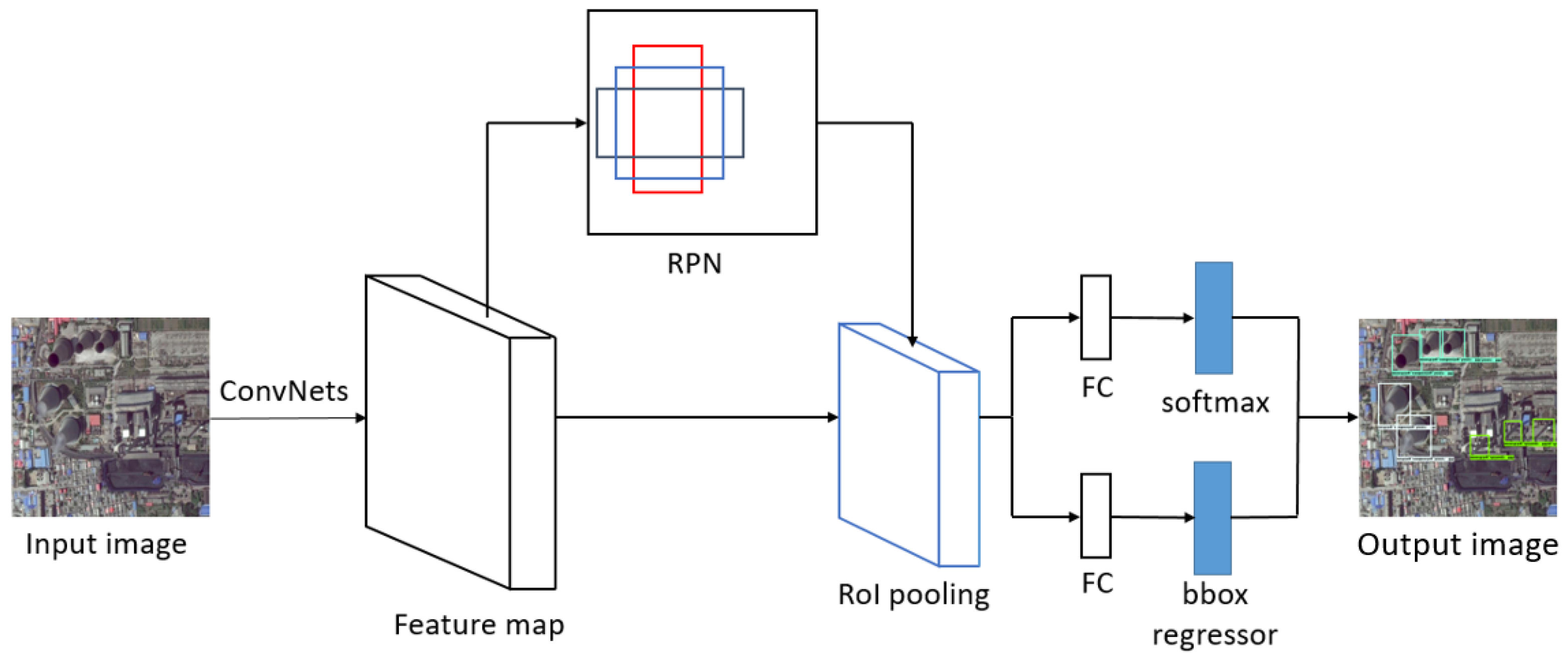
Faster R-CNN [18] is a classic two-stage detector, and the other three two-stage detectors we chose are modified from it. As a two-stage detector, Faster R-CNN has relatively high detection accuracy, but it has relatively high memory cost and running time. As shown in Figure 1, Faster R-CNN uses backbone convolutional networks (ConvNets) to get the feature map of input images firstly. Then, it uses RPN to generate a set of rectangular object proposals with an objectness score for each one. The RoI pooling layers can accelerate the detection process. After fully connected layers (FC), there is a softmax classifier, which determines the class of the targets, and a bounding box regressor, which selects the best bounding box proposals. The detections with relatively low scores will be abandoned by NMS process.
3.1.2. FPN
Compared with Faster R-CNN, FPN [22] has higher detection accuracy at the cost of longer running time and larger memory cost. FPN leverages the pyramidal shape of a ConvNet’s feature hierarchy by creating a feature pyramid that has rich semantics at all levels. The feature pyramid can be built quickly from a single input image scale. As shown in Figure 2, FPN builds a feature pyramid network containing different scales of feature map. The proposal and detection are generated from feature map with different scales instead of only one scale in Faster R-CNN, which is good at detecting targets of different scales.
3.1.3. R-FCN
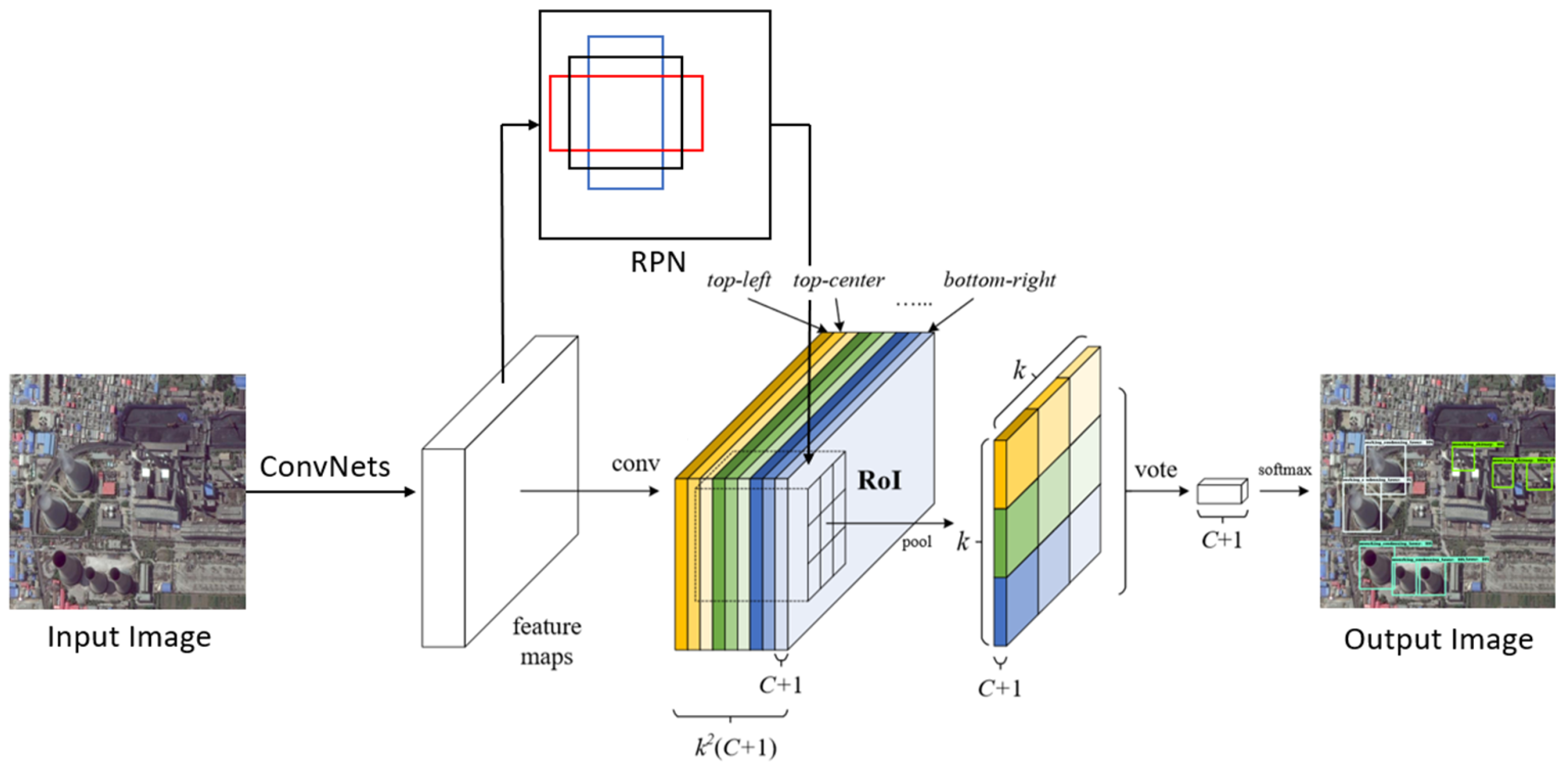
In contrast to FPN, R-FCN [23] runs faster at the cost of lower accuracy. R-FCN is fully convolutional with almost all computation shared on the entire image. As shown in Figure 3, the main difference between Faster R-CNN and R-FCN is in RoI layers. To explicitly encode position information into each RoI, R-FCN divides each RoI rectangle into bins by a regular grid. The last convolutional layer of RoI layers is constructed to produce score maps for each category, and thus has a (C + 1)-channel output layer with C object categories (+1 for background). The bank of score maps correspond to a spatial grid describing relative positions. The position-sensitive scores then vote on the RoI.
3.1.4. DCN
Compared with Faster R-CNN, DCN [24] introduces two new modules to enhance the transformation modeling capability of CNNs, namely deformable convolution and deformable RoI pooling. As illustrated in Figure 4a, offsets are added to the regular grid sampling locations in the standard convolution. As shown in Figure 4b, an offset is added to each bin position in the regular bin partition of the previous RoI pooling. The offsets in two modules are learned from the preceding feature maps.
3.1.5. SSD
SSD [26] is a classic one-stage detector. It runs very quickly and has relatively low memory cost, but its detection accuracy is not as good as two-stage detectors. SSD completely eliminates proposal generation and subsequent feature resampling stages and encapsulates all computation in a single network, which makes it easy to train and straightforward to integrate into systems that require a detection component. As shown in Figure 5, SSD adds convolutional feature layers to the end of the backbone network, which decrease in size progressively and allow predictions of detections at multiple scales. Each added feature layer produces a fixed set of detection predictions using a set of convolutional filters. SSD uses default boxes instead of RPN and anchors. The default boxes tile the feature map in a convolutional manner and the offsets relative to the default box shapes as well as the per-class scores are predicted at each cell.
3.1.6. DSSD
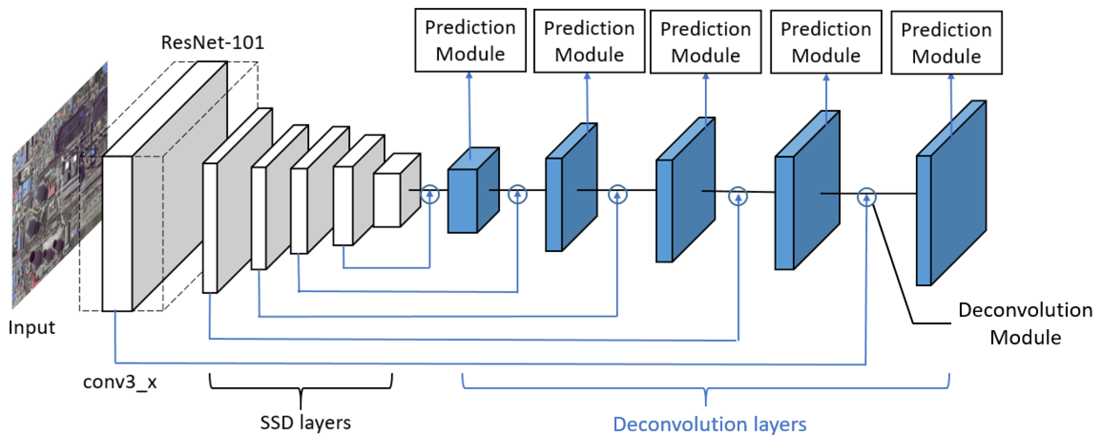
DSSD [28] is modified from SSD and it improves the detection accuracy at the cost of longer running time and larger memory cost. As shown in Figure 6, it augments SSD with prediction module, deconvolution layers and deconvolution modules to introduce additional large scale context in object detection and improve accuracy, especially for small objects. The prediction module adds one residual block to the prediction layer of SSD. To include more high-level context in detection, predictions are moved to a series of deconvolution layers placed after the original SSD layers. To help integrate information from earlier feature maps and the deconvolution layers, deconvolution modules are introduced.
3.1.7. YOLO
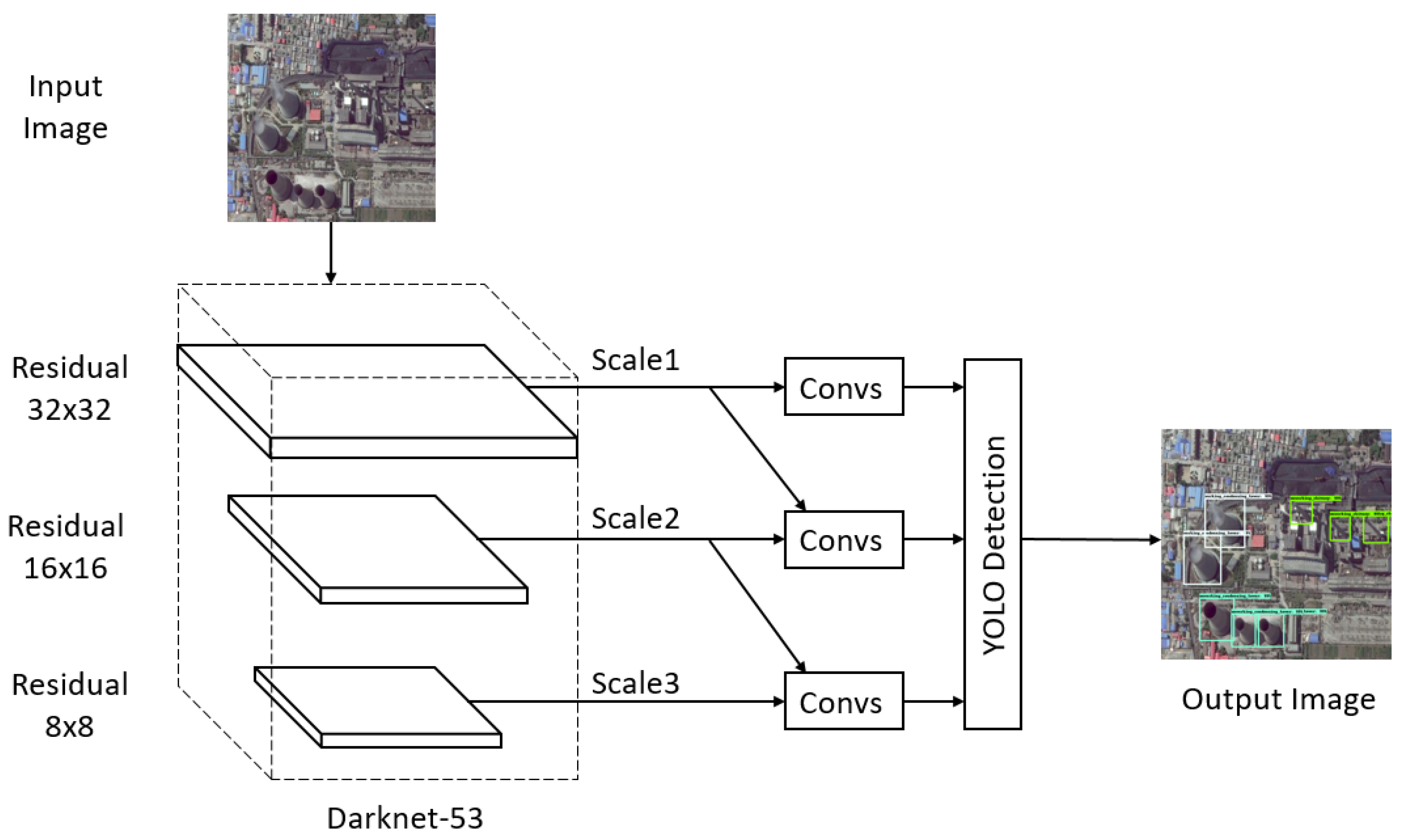
YOLO [27] is also a classic one-stage detector and YOLOv3 [30] is the third version of YOLO, i.e., the state-of-the-art version. YOLOv3 has short running time and its accuracy is close to two-stage detectors. YOLOv3 frames object detection as a regression problem to spatially separated bounding boxes and associated class probabilities. As shown in Figure 7, YOLOv3 predicts boxes at three different scales. YOLOv3 also takes a feature map from earlier in the network and merges it with upsampled features using concatenation. Thus, the predictions for the third scale benefit from all the prior computation. YOLOv3 used k-means clustering to generate nine bounding box priors of our dataset.
3.1.8. RetinaNet
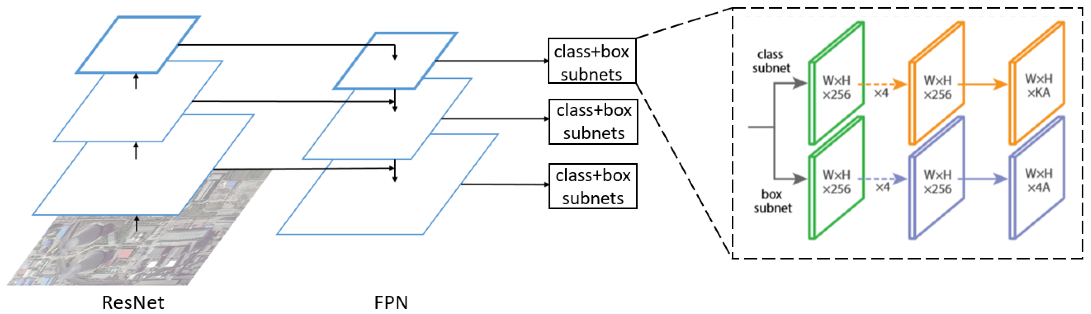
RetinaNet [31] has the advantages of both one-stage detector and two-stage detector, i.e., high accuracy, short running time and small memory cost. RetinaNet uses a novel loss function called focal loss to address the class imbalance problem that most one-stage detectors have. As shown in Figure 8, RetinaNet adopts ResNet-101 [39] with FPN as the backbone network. The classification subnet is a small fully convolutional networks (FCN) attached to each FPN level, which predicts the probability of object presence at each spatial position. In parallel with the classification subnet, the box regression subnet, which is also a small FCN, is attached to each pyramid level for the purpose of regressing the offset from each anchor box.
3.2. Implementation Details
3.2.1. Backbone Network
Backbone network is a basic pre-trained network used to extract features of input images in deep learning based detectors. The backbone network of all eight models except YOLOv3 is ResNet-101 [39], while YOLOv3 uses darknet-53 [30] as its backbone network. We chose ResNet-101 as the backbone of seven models because residual networks can usually achieve better performance than most other backbones on object detection and ResNet-101 is the most widely used network among all the residual networks. We chose darknet-53 as the backbone of YOLOv3 because darknet-53 shows better accuracy than ResNet-101 when applied to YOLOv3 in the original paper of YOLOv3 [30], where darknet-53 is proposed.
ResNet-101 is a 101-layer residual network. Residual learning framework eases the training of deep networks, because it solves the problem of out of convergence and degradation. The layers are reformulated as learning residual functions with reference to the layer inputs, instead of learning unreferenced functions. There is comprehensive empirical evidence showing that the residual networks are easier to optimize, and can gain accuracy from considerably increased depth.
Darknet-53 is a hybrid approach between the network used in YOLOv2, Darknet-19 [29], and residual network. Darknet-53 uses successive 3 × 3 and 1 × 1 convolutional layers and some shortcut connections as well. It has 53 convolutional layers, larger than darknet-19. Darknet-53 also uses batch normalization to stabilize training, speed up convergence, and regularize the model.
3.2.2. Training Details
During the NMS process of eight models, we kept the top-32 ranked proposal regions as final detections. We adjusted the scales and aspect ratios of anchors or default boxes in seven models except YOLOv3, to make them achieve the best performance on our dataset. In detail, the aspect ratios of anchors or default boxes in these seven models were 1:1, 1:2, 2:1, 1:3 and 3:1. The scales of anchors in Faster R-CNN, R-FCN and DCN were 32, 64, 128, and 256 pixels. The anchors had scales of 32 to 512 pixels on pyramid levels P2 to P6, respectively, in FPN. The scales of default boxes varied from 0.2 × 512 × 512 to 0.9 × 512 × 512 pixels in different feature maps in both SSD and DSSD. The anchors had scales of 32 to 512 pixels on pyramid levels P3 to P7, respectively, in RetinaNet. As an exception, YOLOv3 generated nine bounding box priors of our dataset automatically by k-means cluster before training. The nine bounding box priors were 31 × 27, 35 × 42, 47 × 70, 62 × 41, 72 × 120, 76 × 69, 110 × 89, 111 × 49 and 137 × 128 pixels.
Other training details of the eight models are shown in Table 2, where such settings of training were chosen to achieve their best performance on our dataset. We used learning rate warm-up method on some models. This method could warm up the models by using small learning rate at the beginning of training. We set the train step big enough to ensure that all models could be thoroughly trained. We chose proper initial learning rate (lr) to make the training process faster and to avoid the problem of out of convergence and gradient explosion. There are three learning rate schedule strategies, i.e., STEP, EXPONENTIAL and ADAM [40]. STEP means that the learning rate keeps the same until the step reaches a certain value. EXPONENTIAL means that the learning rate is an exponential function of steps. ADAM is a method for stochastic optimization which is more complicated. The batch sizes of two-stage detectors were all 1, while the batch sizes of one-stage detectors were different. Besides, all models used pre-trained weights to fine-tune, which saved a lot of training time.
4. Experimental Results
To ensure the fairness of comparison, we trained and tested the eight models, namely Faster R-CNN [18], FPN [22], R-FCN [23], DCN [24], SSD [26], DSSD [28], YOLOv3 [30], and RetinaNet [31], on the same hardware, which is a server with a 2.5 GHz Central Processing Unit (CPU) and a Nvidia Tesla P4 Graphics Processing Unit (GPU). The memory of CPU and GPU is 16 GB and 8 GB, respectively. We used the same training data to train the eight models and test the learned models with the same testing data as well.
4.1. BUAA-FFPP60 Dataset
Based on the data provided in [4], which contain 217 power plant images of 1-m spatial resolution with labeled locations and classes of chimney or condensing tower, we added 101 new images with 1-m spatial resolution collected from Google Earth and built a more comprehensive dataset named BUAA-FFPP60, meaning that it contains RSIs of over 60 fossil-fuel power plants (FFPP) collected by researchers from Beihang University (BUAA). BUAA-FFPP60 contains 1-m spatial resolution RSIs of over 60 fossil-fuel power plants in the Beijing-Tianjin-Hebei region in North China, which covers about 123 km in urban areas. The size of 318 original images under different imaging conditions varies from to pixels. Thirty-one images were selected as the testing data, the same as in [4]. The remaining 287 RSIs were augmented by mirroring and rotating, resulting in a training set of 861 images. Comparing to the dataset used in [4], BUAA-FFPP60 contains not only locations and two-class labels but also working status labels (four-class), which makes it possible to achieve the whole task of power plant monitoring, not as the sub-task of power plant detection in [4]. The working status of chimney or condensing tower is determined by their emission of smoke. The statistics of BUAA-FFPP60 dataset is illustrated in Table 3, and Figure 9 shows the image samples. It should be noticed that our BUAA-FFPP60 RSI dataset is released to the public. It is available from the corresponding author upon request or via the website (https://github.com/SPDQ/Power-Plant-Detection-in-RSI).
4.2. Index for Evaluation
To evaluate the detection accuracy of the eight models, we used four popular indicators: precision, recall, average precision (AP) and mean average precision (mAP). These indicators are computed based on IoU. IoU is the ratio between the intersection of the predict bounding box (), ground truth (), and the union of them, i.e.,
When IoU exceeds a threshold, the bounding box is considered to be correct. We set the value of threshold as 0.5, the same as in [36], which means at least half of the predicted box covers the same region as the ground truth. When IoU is greater than 0.5, the test result is a true positive (TP), and when the value is less than 0.5, it is called a false positive (FP). The false negative (FN) indicates that the model predicts that there is no target in the image, but actually the image does contain a target. Then, we can combine these into two metrics, precision (P) and recall (R), as
P measures the fraction of true positives (TP) in all the detections, while R is the ratio of true positives (TP) to the total number of targets in ground truth.
The output of deep learning based detectors contains detections and their scores. The scores represent how confident the detector is about the detection. After sorting detections by scores from high to low and computing the precision and recall of all the detections, we can draw a precision–recall curve (PRC) which is a plot of P as a function of R. The average precision is the area under the PRC, and is more comprehensive for performance evaluation. The average value of AP for all kinds of targets is mAP. Our evaluation method is based on COCO metric API, which is available online (https://github.com/cocodataset/cocoapi).
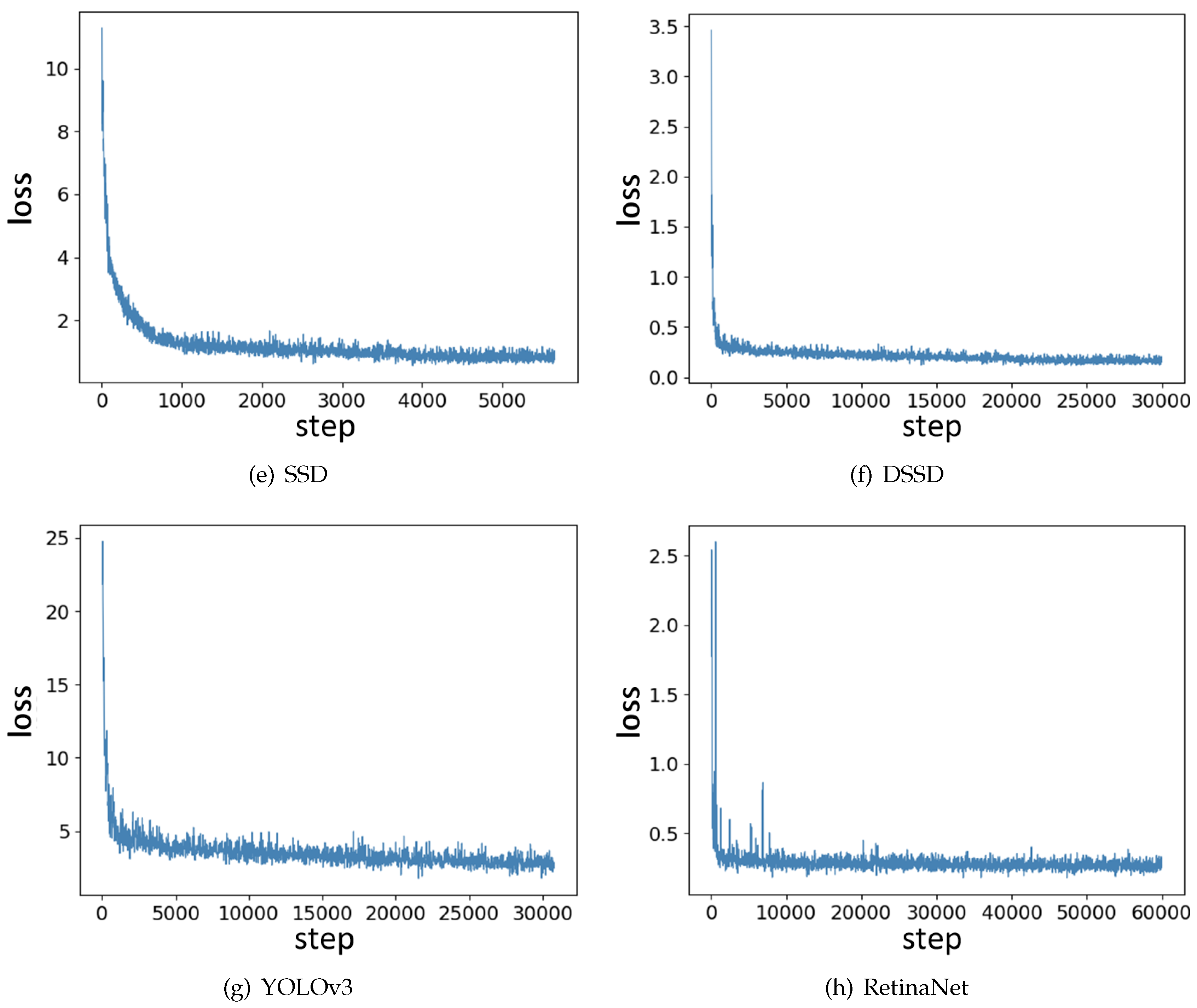
4.3. Training Loss
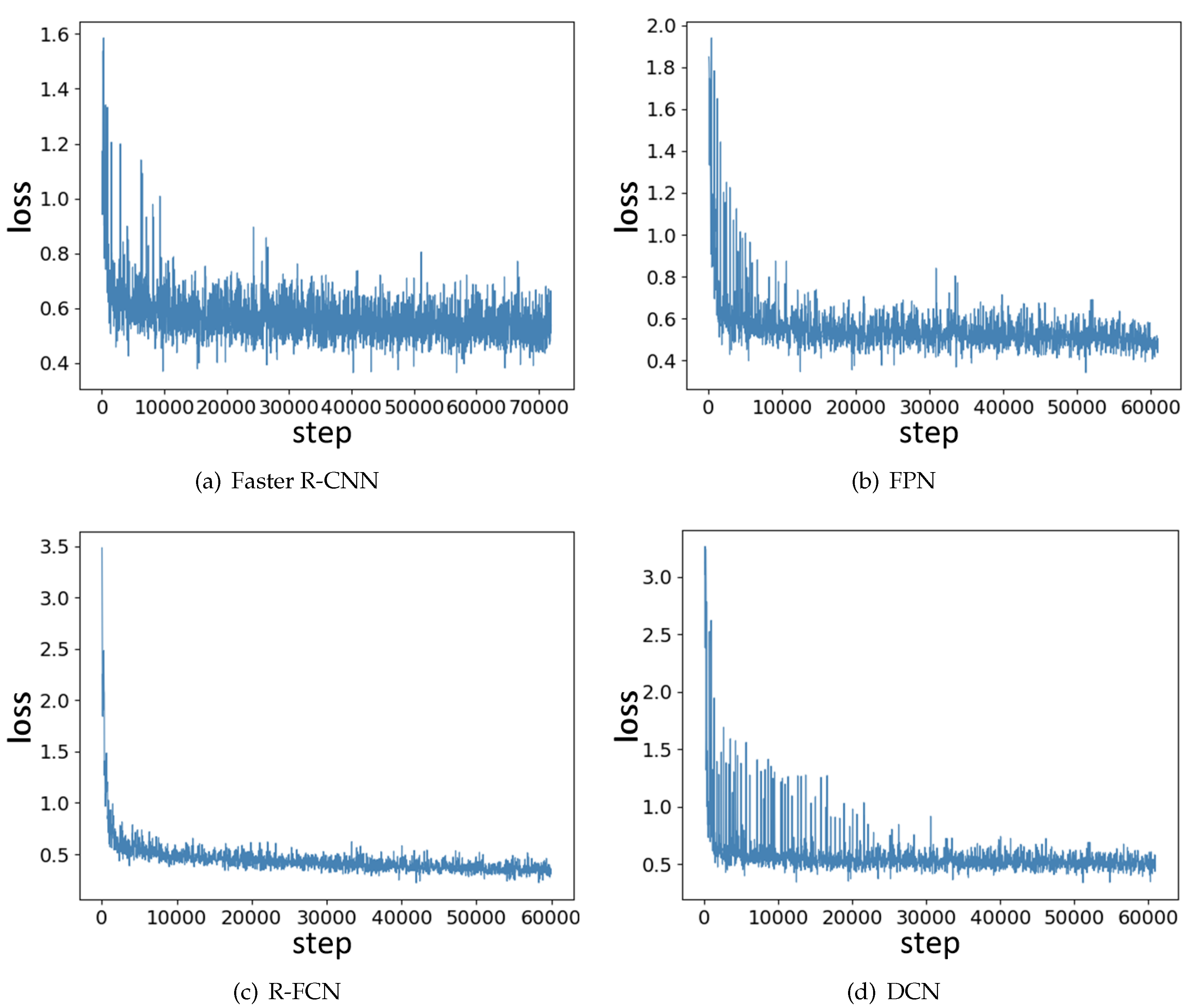
The change of loss during training is shown in Figure 10. We found that one-stage models including SSD, DSSD, YOLOv3 and RetinaNet converged more quickly than two-stage models. R-FCN had more robust training loss than Faster R-CNN, FPN and DCN, of which the training loss kept fluctuating for many steps. Although there were some difference in the training process, all eight models reached the minimum loss and their loss Was stable in a small range, meaning that they were all trained thoroughly.
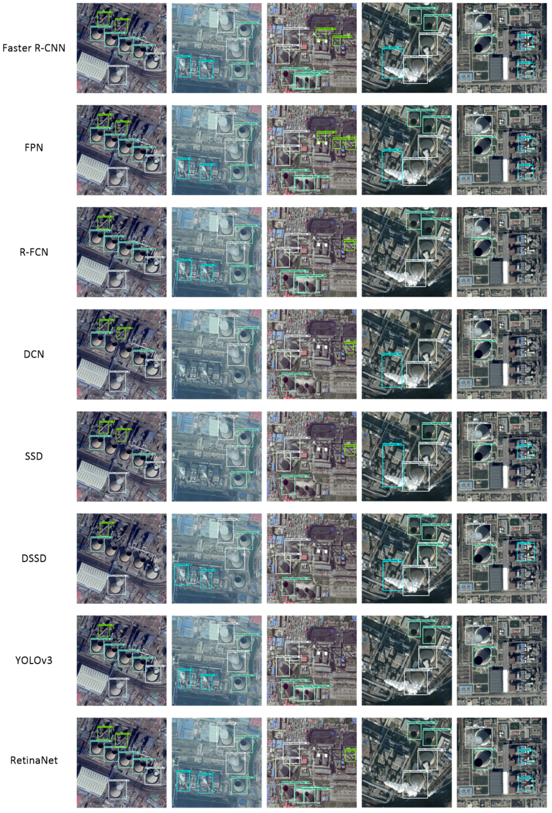
4.4. Accuracy Comparison
We report the quantitative accuracy of eight deep learning models for a sub-task of power plant detection in Table 4 and the whole task of power plant monitoring in Table 5. A qualitative visualization is shown in Figure 11. In Table 4, we can see that Faster R-CNN, FPN and RetinaNet outperformed Yao et al. [4] in chimney and condensing tower detection. Although Yao et al. [4] also used Faster R-CNN model, our Faster R-CNN performed better owing to the adjustment of aspect ratios of anchor, the training data augment, and more comprehensive class labels.
As shown in Table 5 and Figure 11, Faster R-CNN, FPN and RetinaNet had relatively high detection accuracy and FPN had the best mean average precision (0.8273). The detection accuracy of DCN and DSSD was relatively low. It can be seen in the tables that, although the accuracies were different, all eight deep learning models could effectively complete the mission of locating power plants and determining their working status.
4.5. Model Size and Memory Cost
In addition to detection accuracy, the space occupancy and memory cost are two important factors to evaluate the performance of models when hardware resource is limited, especially in the case that deep learning models are applied to computers or mobile devices with limited space and memory. The space occupancy is the disk storage space occupied by saved parameters of trained models. The space occupancy can reflect the parameter number and complexity of models. The memory cost shows how much GPU memory is used when detecting objects in a RSI. The memory cost reflects the GPU dependence of models. The space occupancy and memory cost of eight models are shown in Table 6. SSD, DSSD and YOLOv3 had relatively small space occupancy, and SSD, DSSD and DCN had relatively low memory cost. SSD needed the smallest space occupancy and memory cost. The three models with high accuracy, i.e., Faster R-CNN, FPN and RetinaNet, did not have a good performance in space occupancy and memory cost. It was difficult to achieve both high accuracy and low memory cost.
4.6. Running Time
Running time is an important factor for practical application, since the high resolution remote sensing usually covers a large areas and generates a large amount of images to be processed. If a model costs less time to run, it has better efficiency to get rapid processing results, which is valuable in emergency task. To reduce measurement error of running time, we computed the sum of running time of all testing RSIs, and report the average running time for the process of image data within 1 km. The running time of eight models is shown in Table 7. SSD, YOLOv3 and RetinaNet ran relatively quickly, and RetinaNet ran the fastest. Although FPN and Faster R-CNN had relatively high accuracy, they were the slowest models. RetinaNet was the only model that could achieve both high accuracy and low running time, although it had the most space occupancy. The fastest RetinaNet could process the 1-m spatial resolution data of whole Beijing-Tianjin-Hebei region within a single day, just about 20 h.
5. Discussion
The analysis of advantages and disadvantages of each deep learning model can help choose the most suitable model to do power plant monitoring work. As shown in Section 4, Faster R-CNN [18] had a high detection accuracy, but it had the biggest space occupancy, big memory cost and long running time. FPN [22] achieved the highest detection accuracy, but it cost the longest running time and needed a relatively big block of model storage space and GPU memory. The detection accuracy of R-FCN [23] seemed good, but its space occupancy and memory cost were relatively high and R-FCN could not run as quickly as one-stage models. DCN [24] needed low memory cost, but it did not have a good performance on other aspects. SSD [26] cost the least memory among all eight models and was also a fast runner with the least model size, at the expenses of worst detection accuracy. DSSD [28] had low space occupancy and memory cost, but its accuracy and running time were not good. YOLOv3 [30] had low running time and space occupancy, while its performance on memory cost and accuracy were not good. Although the model size of RetinaNet [31] was the biggest, its performance was balanced on both high accuracy and low running time. If accuracy is given top priority, Faster R-CNN [18], FPN [22], and RetinaNet [31] are suggested for application, since they could perform mean average precision over 80%. If the hardware resource, especially the memory of GPU, is limited, DCN [24] and SSD [26] can be taken in to consideration. RetinaNet [31] ran the fastest among the eight models, thus could be used to get rapid results. We could not find a model that has a good performance on all aspects, thus we need to choose the most suitable model based on the requirements and restrictions in practical situation.
Our work effectively completed the mission of power plant localization and classification, but the detection accuracy of chimney was not good enough and we could not find a model with good performance on all aspects. This is because all models compared in this study were fine-tuned from their original networks with best selected parameters and settings. To improve the current work, the structures of the eight models should be specially adjusted to be suitable for the task of power plant monitoring, especially to make them achieve a better performance in all aspects based on our experimental results.
As the rapid development of satellite based and airborne Earth observing, high resolution remote sensing data can be obtained more and more easily. The high performance–price ratio of unmanned aircrafts and commercial micro-nano satellites make it available to acquire very high resolution remote sensing data of the regions of interest at low cost and high frequency. Thus, given high resolution remote sensing data of fossil-fuel power plants, our deep learning based framework can automatically detect the power plants and determine their working status for monitoring urban environment around fossil-fuel power plants. The experimental results in Section 4 validate the effectiveness and feasibility of our framework for 1-m spatial resolution Google Earth data. Considering the good generalization ability of deep learning models, our framework has significant potential for fossil-fuel power plant monitoring using high resolution remote sensing data, benefiting the control of the anthropogenic emission and air quality.
6. Conclusions
In this paper, we have proposed a deep learning based framework to complete the mission of fossil-fuel power plant monitoring via simultaneously locating the power plants and determining their working status in high resolution optical remote sensing images. A RSI dataset named BUAA-FFPP60 has been released to the public, which consists of 1-m spatial resolution images collected from Google Earth in about 123 km urban areas of the Beijing-Tianjin-Hebei region in North China. Eight state-of-the-art deep learning models, namely Faster R-CNN [18], FPN [22], R-FCN [23], DCN [24], SSD [26], DSSD [28], YOLOv3 [30] and RetinaNet [31], were trained and tested on BUAA-FFPP60. Comprehensive comparative experiments demonstrate the effectiveness of deep learning for fossil-fuel power plant localization and working status determination. Considering the trade-off among accuracy, speed and hardware cost, we suggest using RetinaNet [31] model in practical application of urban environment monitoring around fossil-fuel power plants.
Author Contributions
Conceptualization, H.Z.; methodology, H.Z. and Q.D.; software, Q.D.; validation, H.Z. and Q.D.; formal analysis, H.Z. and Q.D.; investigation, H.Z. and Q.D.; resources, H.Z. and Q.D.; data curation, H.Z. and Q.D.; writing—original draft preparation, H.Z. and Q.D.; writing—review and editing, H.Z.; visualization, Q.D.; supervision, H.Z.; project administration, H.Z.; and funding acquisition, H.Z.
Funding
This work was supported in part by the National Natural Science Foundation of China (Grant Nos. 61771031, 61501009, and 61371134), the National Key Research and Development Program of China (Grant Nos. 2016YFB0501300 and 2016YFB0501302), and the Fundamental Research Funds for the Central Universities.
Conflicts of Interest
The authors declare no conflict of interest. The funders had no role in the design of the study; in the collection, analyses, or interpretation of data; in the writing of the manuscript, or in the decision to publish the results.
References
- He, X.; Xue, Y.; Guang, J.; Shi, Y.; Xu, H.; Cai, J.; Mei, L.; Li, C. The analysis of the haze event in the north china plain in 2013. In Proceedings of the IEEE International Geoscience and Remote Sensing Symposium (IGARSS), Quebec City, QC, Canada, 13–18 July 2014; pp. 5002–5005. [Google Scholar] [CrossRef]
- Feng, X.; Li, Q.; Zhu, Y. Bounding the role of domestic heating in haze pollution of beijing based on satellite and surface observations. In Proceedings of the IEEE International Geoscience and Remote Sensing Symposium (IGARSS), Quebec City, QC, Canada, 13–18 July 2014; pp. 5727–5728. [Google Scholar] [CrossRef]
- Kai, Q.; Hu, M.; Lixin, W.; Rao, L.; Lang, H.; Wang, L.; Yang, B. Satellite remote sensing of aerosol optical depth, SO2 and NO2 over China’s Beijing-Tianjin-Hebei region during 2002–2013. In Proceedings of the IEEE International Geoscience and Remote Sensing Symposium (IGARSS), Beijing, China, 10–15 July 2016; pp. 5727–5728. [Google Scholar] [CrossRef]
- Yao, Y.; Jiang, Z.; Zhang, H.; Cai, B.; Meng, G.; Zuo, D. Chimney and condensing tower detection based on faster R-CNN in high resolution remote sensing images. In Proceedings of the IEEE International Geoscience and Remote Sensing Symposium (IGARSS), Fort Worth, TX, USA, 23–28 July 2017; pp. 3329–3332. [Google Scholar] [CrossRef]
- Zhang, F.; Du, B.; Zhang, L.; Xu, M. Weakly supervised learning based on coupled convolutional neural networks for aircraft detection. IEEE Trans. Geosci. Remote Sens. 2016, 5553–5563. [Google Scholar] [CrossRef]
- Cai, B.; Jiang, Z.; Zhang, H.; Yao, Y.; Nie, S. Online Exemplar-Based Fully Convolutional Network for Aircraft Detection in Remote Sensing Images. IEEE Geosci. Remote Sens. Lett. 2018, 15, 1095–1099. [Google Scholar] [CrossRef]
- Zou, Z.; Shi, Z. Ship detection in spaceborne optical image with svd networks. IEEE Trans. Geosci. Remote Sens. 2016, 5832–5845. [Google Scholar] [CrossRef]
- Yao, Y.; Jiang, Z.; Zhang, H.; Zhao, D.; Cai, B. Ship detection in optical remote sensing images based on deep convolutional neural networks. J. Appl. Remote Sens. 2017, 11, 11–12. [Google Scholar] [CrossRef]
- Yang, X.; Sun, H.; Fu, K.; Yang, J.; Sun, X.; Yan, M.; Guo, Z. Automatic Ship Detection in Remote Sensing Images from Google Earth of Complex Scenes Based on Multiscale Rotation Dense Feature Pyramid Networks. Remote Sens. 2018, 10, 132. [Google Scholar] [CrossRef]
- Zhang, L.; Shi, Z.; Wu, J. A Hierarchical Oil Tank Detector With Deep Surrounding Features for High-Resolution Optical Satellite Imagery. IEEE J. Sel. Top. Appl. Earth Obs. Remote Sens. 2015, 8, 4895–4909. [Google Scholar] [CrossRef]
- Yao, Y.; Jiang, Z.; Zhang, H. Oil tank detection based on salient region and geometric features. Proc. SPIE 2016, 92731G. [Google Scholar] [CrossRef]
- Wang, W.; Zhao, D.; Jiang, Z. Oil Tank Detection via Target-Driven Learning Saliency Model. In Proceedings of the 2017 4th IAPR Asian Conference on Pattern Recognition (ACPR), Nanjing, China, 26–29 November 2017; pp. 156–161. [Google Scholar] [CrossRef]
- Zhu, X.X.; Tuia, D.; Mou, L.; Xia, G.; Zhang, L.; Xu, F.; Fraundorfer, F. Deep Learning in Remote Sensing: A Comprehensive Review and List of Resources. IEEE Geosci. Remote Sens. Mag. 2017, 5, 8–36. [Google Scholar] [CrossRef] [Green Version]
- Han, G.C.J. A survey on object detection in optical remote sensing images. ISPRS J. Photogramm. Remote Sens. 2016, 11–28. [Google Scholar] [CrossRef]
- Zou, Z.; Shi, Z. Random Access Memories: A New Paradigm for Target Detection in High Resolution Aerial Remote Sensing Images. IEEE Trans. Image Process. 2018, 27, 1100–1111. [Google Scholar] [CrossRef] [PubMed]
- Xia, G.S.; Bai, X.; Ding, J.; Zhu, Z.; Belongie, S.; Luo, J.; Datcu, M.; Pelillo, M.; Zhang, L. DOTA: A Large-Scale Dataset for Object Detection in Aerial Images. In Proceedings of the The IEEE Conference on Computer Vision and Pattern Recognition (CVPR), Salt Lake, UT, USA, 18–22 June 2018. [Google Scholar]
- Ding, J.; Xue, N.; Long, Y.; Xia, G.S.; Lu, Q. Learning RoI Transformer for Detecting Oriented Objects in Aerial Images. In Proceedings of the IEEE Conference on Computer Vision and Pattern Recognition (CVPR), Long Beach, CA, USA, 16–20 June 2019. [Google Scholar]
- Ren, S.; He, K.; Girshick, R.; Sun, J. Faster R-CNN: Towards Real-Time Object Detection with Region Proposal Networks. In Advances in Neural Information Processing Systems 28; Cortes, C., Lawrence, N.D., Lee, D.D., Sugiyama, M., Garnett, R., Eds.; Curran Associates, Inc.: Red Hook, NY, USA, 2015; pp. 91–99. [Google Scholar]
- Girshick, R.; Donahue, J.; Darrell, T.; Malik, J. Rich Feature Hierarchies for Accurate Object Detection and Semantic Segmentation. In Proceedings of the 2014 IEEE Conference on Computer Vision and Pattern Recognition, Columbus, OH, USA, 23–28 June 2014; pp. 580–587. [Google Scholar] [CrossRef]
- He, K.; Zhang, X.; Ren, S.; Sun, J. Spatial Pyramid Pooling in Deep Convolutional Networks for Visual Recognition. IEEE Trans. Pattern Anal. Mach. Intell. 2015, 37, 1904–1916. [Google Scholar] [CrossRef] [PubMed]
- Girshick, R. Fast R-CNN. In Proceedings of the 2015 IEEE International Conference on Computer Vision (ICCV), Santiago, Chile, 7–13 December 2015; pp. 1440–1448. [Google Scholar] [CrossRef]
- Lin, T.; Dollár, P.; Girshick, R.; He, K.; Hariharan, B.; Belongie, S. Feature Pyramid Networks for Object Detection. In Proceedings of the 2017 IEEE Conference on Computer Vision and Pattern Recognition (CVPR), Honolulu, HI, USA, 21–26 July 2017; pp. 936–944. [Google Scholar] [CrossRef]
- Dai, J.; Li, Y.; He, K.; Sun, J. R-FCN: Object Detection via Region-based Fully Convolutional Networks. In Advances in Neural Information Processing Systems 29; Lee, D.D., Sugiyama, M., Luxburg, U.V., Guyon, I., Garnett, R., Eds.; Curran Associates, Inc.: Red Hook, NY, USA, 2016; pp. 379–387. [Google Scholar]
- Dai, J.; Qi, H.; Xiong, Y.; Li, Y.; Zhang, G.; Hu, H.; Wei, Y. Deformable Convolutional Networks. In Proceedings of the 2017 IEEE International Conference on Computer Vision (ICCV), Venice, Italy, 22–29 October 2017; pp. 764–773. [Google Scholar] [CrossRef]
- Sermanet, P.; Eigen, D.; Zhang, X.; Mathieu, M.; Fergus, R.; Lecun, Y. OverFeat: Integrated Recognition, Localization and Detection using Convolutional Networks. In Proceedings of the ICLR 2014, Banff, AB, Canada, 14–16 April 2014. [Google Scholar]
- Liu, W.; Anguelov, D.; Erhan, D.; Szegedy, C.; Reed, S.; Fu, C.Y.; Berg, A.C. SSD: Single Shot MultiBox Detector. In Computer Vision–ECCV 2016; Leibe, B., Matas, J., Sebe, N., Welling, M., Eds.; Springer International Publishing: Cham, Switzerland, 2016; pp. 21–37. [Google Scholar]
- Redmon, J.; Divvala, S.K.; Girshick, R.B.; Farhadi, A. You Only Look Once: Unified, Real-Time Object Detection. In Proceedings of the 2016 IEEE Conference on Computer Vision and Pattern Recognition (CVPR), Las Vegas, NV, USA, 26 June–1 July 2016; pp. 779–788. [Google Scholar] [CrossRef]
- Fu, C.Y.; Liu, W.; Ranga, A.; Tyagi, A.; Berg, A.C. DSSD: Deconvolutional Single Shot Detector. arXiv 2017, arXiv:1701.06659. [Google Scholar]
- Redmon, J.; Farhadi, A. YOLO9000: Better, Faster, Stronger. In Proceedings of the 2017 IEEE Conference on Computer Vision and Pattern Recognition (CVPR), Honolulu, HI, USA, 21–26 July 2017; pp. 6517–6525. [Google Scholar] [CrossRef]
- Redmon, J.; Farhadi, A. YOLOv3: An Incremental Improvement. arXiv 2018, arXiv:1804.02767. [Google Scholar]
- Lin, T.; Goyal, P.; Girshick, R.; He, K.; Dollár, P. Focal Loss for Dense Object Detection. In Proceedings of the 2017 IEEE International Conference on Computer Vision (ICCV), Venice, Italy, 22–29 October 2017; pp. 2999–3007. [Google Scholar] [CrossRef]
- Xu, Z.; Xu, X.; Wang, L.; Yang, R.; Pu, F. Deformable ConvNet with Aspect Ratio Constrained NMS for Object Detection in Remote Sensing Imagery. Remote Sens. 2017, 9, 1312. [Google Scholar] [CrossRef]
- Ren, Y.; Zhu, C.; Xiao, S. Deformable Faster R-CNN with Aggregating Multi-Layer Features for Partially Occluded Object Detection in Optical Remote Sensing Images. Remote Sens. 2018, 10, 1470. [Google Scholar] [CrossRef]
- Liu, X.; Tian, Y.; Yuan, C.; Zhang, F.; Yang, G. Opium Poppy Detection Using Deep Learning. Remote Sens. 2018, 10, 1886. [Google Scholar] [CrossRef]
- Tao, Y.; Xu, M.; Zhang, F.; Du, B.; Zhang, L. Unsupervised-Restricted Deconvolutional Neural Network for Very High Resolution Remote-Sensing Image Classification. IEEE Trans. Geosci. Remote Sens. 2017, 55, 6805–6823. [Google Scholar] [CrossRef]
- Chang, Y.L.; Anagaw, A.; Chang, L.; Wang, Y.C.; Hsiao, C.Y.; Lee, W.H. Ship Detection Based on YOLOv2 for SAR Imagery. Remote Sens. 2019, 11, 786. [Google Scholar] [CrossRef]
- Wang, Y.; Wang, C.; Zhang, H.; Dong, Y.; Wei, S. Automatic Ship Detection Based on RetinaNet Using Multi-Resolution Gaofen-3 Imagery. Remote Sens. 2019, 11, 531. [Google Scholar] [CrossRef]
- Foody, G.M.; Ling, F.; Boyd, D.S.; Li, X.; Wardlaw, J. Earth Observation and Machine Learning to Meet Sustainable Development Goal 8.7: Mapping Sites Associated with Slavery from Space. Remote Sens. 2019, 11, 266. [Google Scholar] [CrossRef]
- He, K.; Zhang, X.; Ren, S.; Sun, J. Deep Residual Learning for Image Recognition. In Proceedings of the 2016 IEEE Conference on Computer Vision and Pattern Recognition (CVPR), Las Vegas, NV, USA, 26 June–1 July 2016; pp. 770–778. [Google Scholar] [CrossRef]
- Kingma, D.P.; Ba, J. Adam: A Method for Stochastic Optimization. In Proceedings of the ICLR 2014, Banff, AB, Canada, 14–16 April 2014. [Google Scholar]
Figure 1.
The framework of Faster R-CNN. RPN, region proposal network; RoI, region of interest; FC, fully connected layer; bbox, bounding box.
Figure 1.
The framework of Faster R-CNN. RPN, region proposal network; RoI, region of interest; FC, fully connected layer; bbox, bounding box.

Figure 2.
The framework of FPN. FPN, feature pyramid network; RPN, region proposal network; RoI, region of interest; FC, fully connected layer; bbox, bounding box.
Figure 2.
The framework of FPN. FPN, feature pyramid network; RPN, region proposal network; RoI, region of interest; FC, fully connected layer; bbox, bounding box.
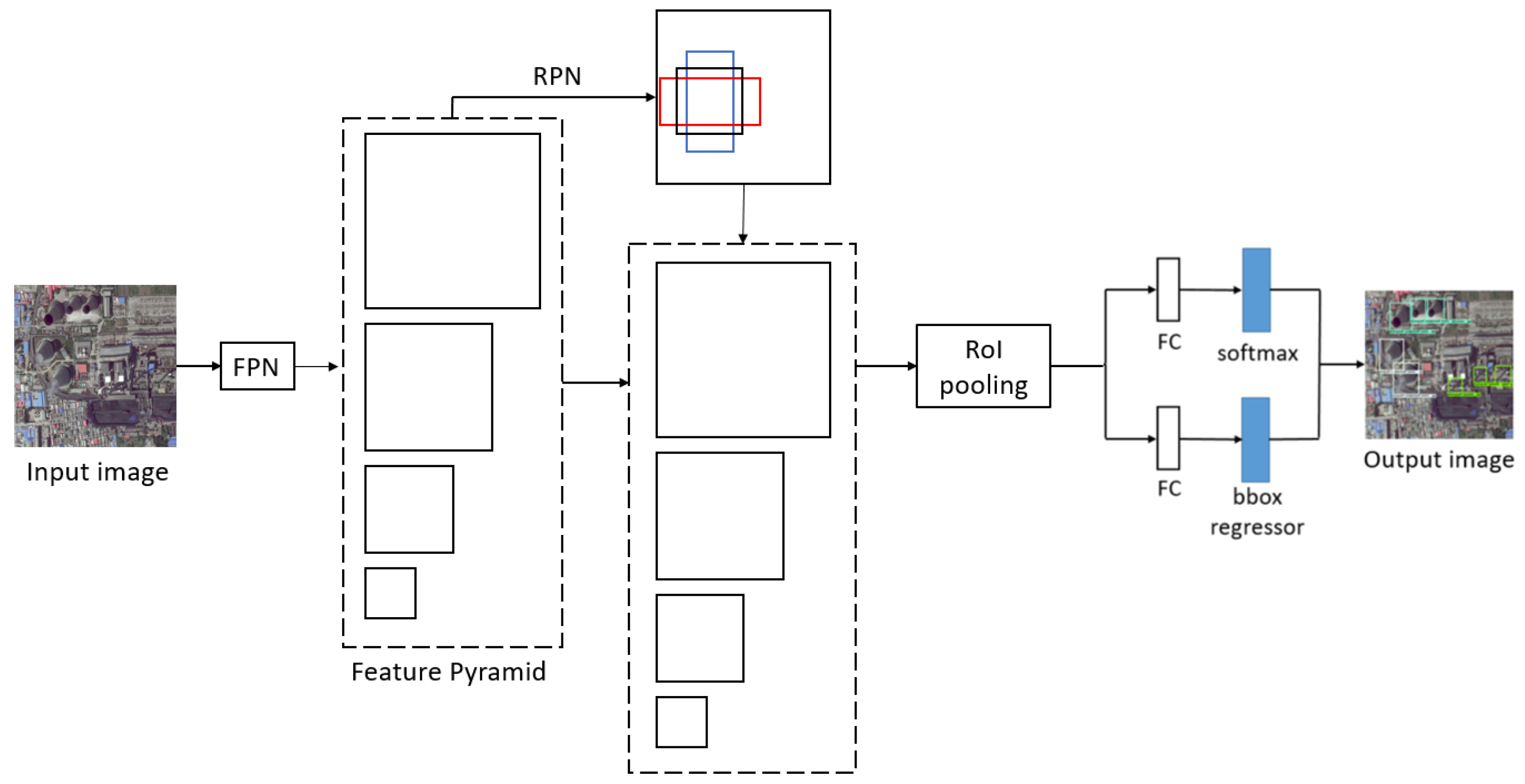
Figure 3.
The framework of R-FCN. RPN, region proposal network; RoI, region of interest; ConvNets and conv, convolutional network.
Figure 3.
The framework of R-FCN. RPN, region proposal network; RoI, region of interest; ConvNets and conv, convolutional network.

Figure 4.
The framework of DCN. Conv, convolutional network; RoI, region of interest; fc, fully connected layer.
Figure 4.
The framework of DCN. Conv, convolutional network; RoI, region of interest; fc, fully connected layer.
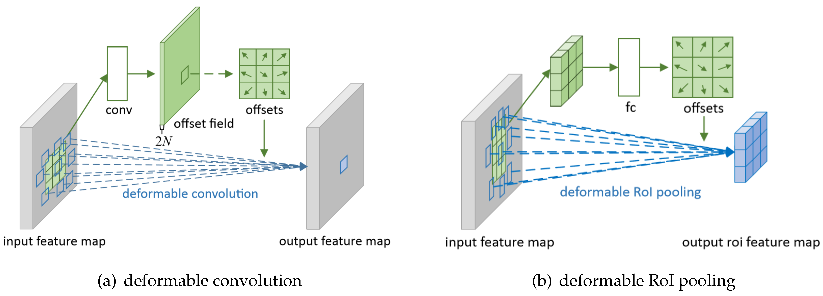
Figure 5.
The framework of SSD. Conv, convolutional networks.
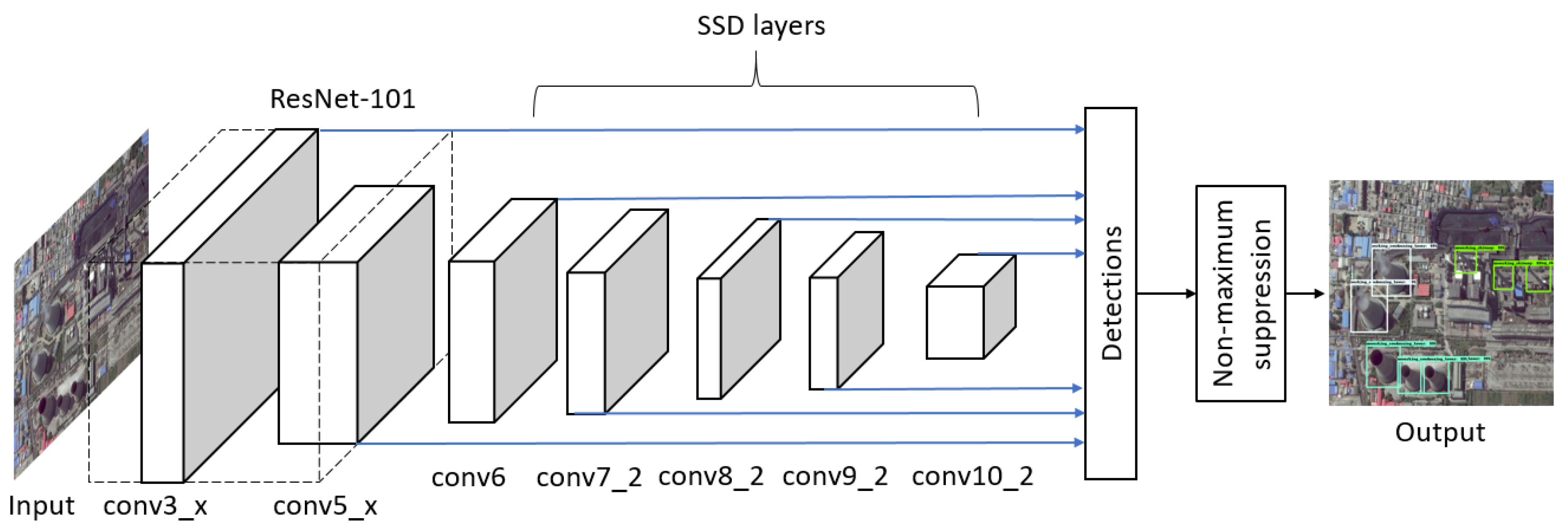
Figure 6.
The framework of DSSD. Conv, convolutional network.

Figure 7.
The framework of YOLOv3. Convs, convolutional networks.

Figure 8.
The framework of RetinaNet. FPN, feature pyramid network.

Figure 9.
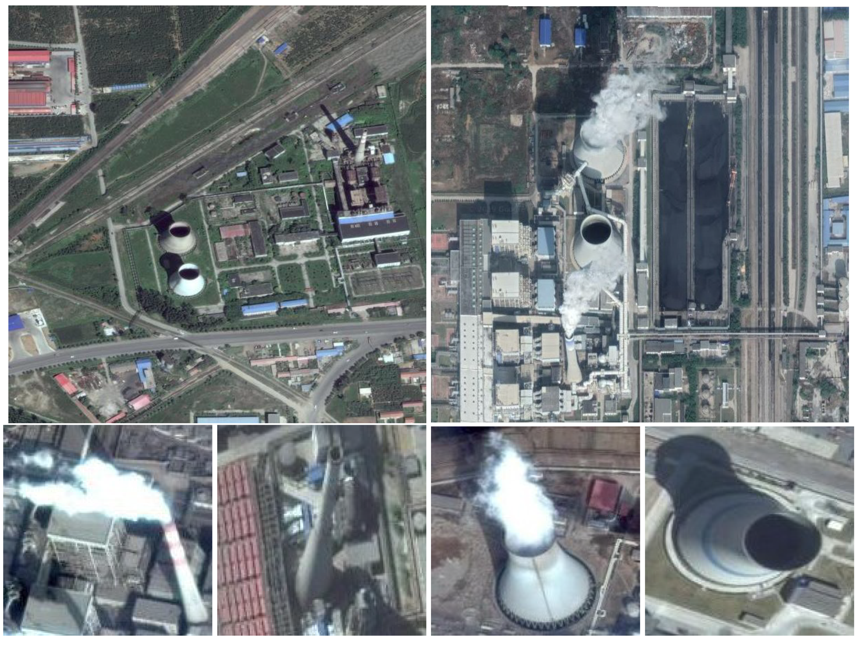
RSI samples in BUAA-FFPP60 dataset. The first two rows show RSIs. The last row shows cropped targets, where the columns from left to right represent working chimneys, non-working chimneys, working condensing towers and non-working condensing towers, respectively.
Figure 9.
RSI samples in BUAA-FFPP60 dataset. The first two rows show RSIs. The last row shows cropped targets, where the columns from left to right represent working chimneys, non-working chimneys, working condensing towers and non-working condensing towers, respectively.
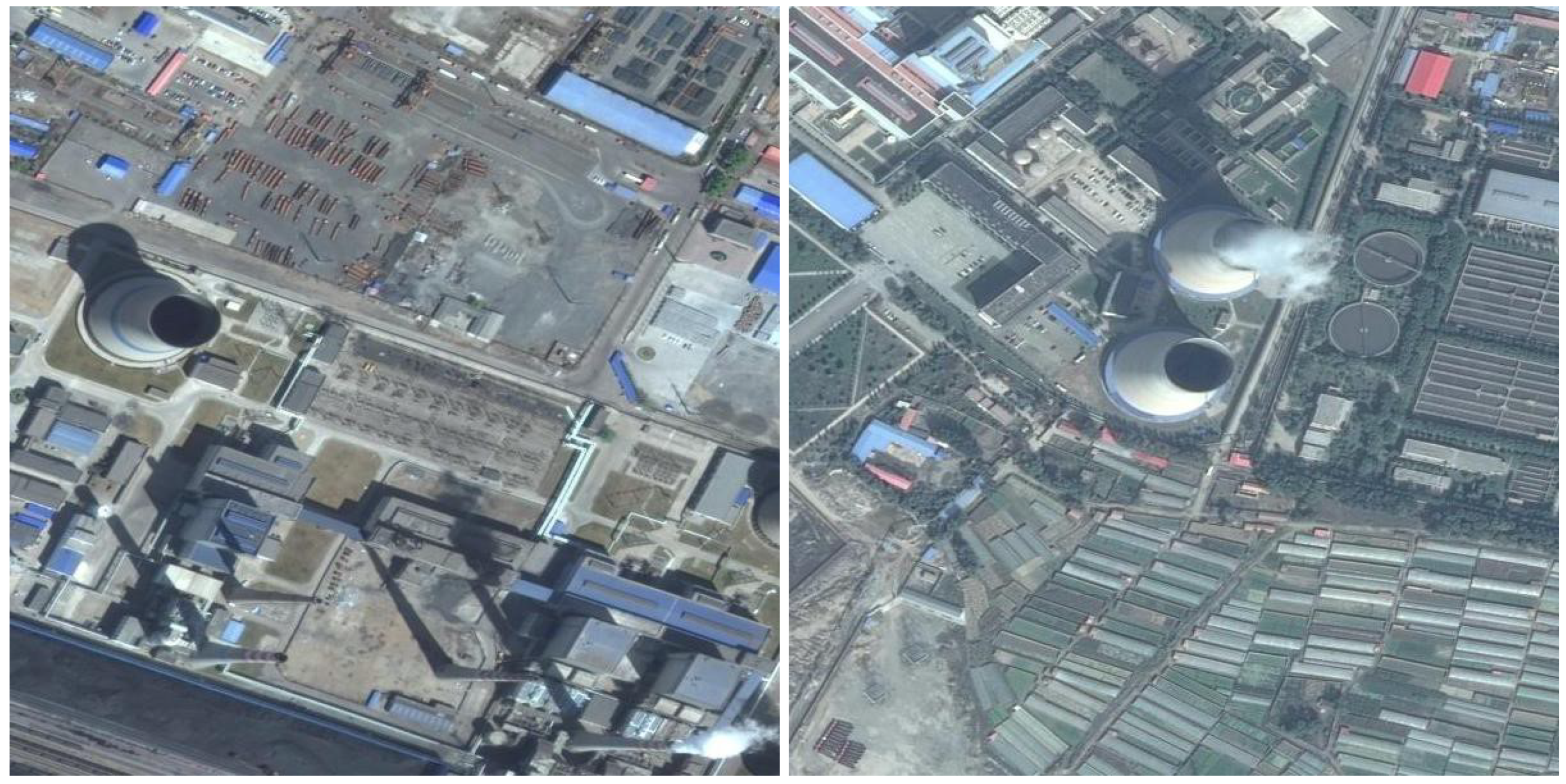

Figure 10.
Changes of loss with steps during training.


Figure 11.
Samples of four-class detection results of eight deep learning models. The white boxes represent working condensing tower, the light blue boxes represent non-working condensing tower, the blue boxes represent working chimney, and the green boxes represent non-working chimney.
Figure 11.
Samples of four-class detection results of eight deep learning models. The white boxes represent working condensing tower, the light blue boxes represent non-working condensing tower, the blue boxes represent working chimney, and the green boxes represent non-working chimney.


Table 1.
Information of eight models.
| Model | Backbone | Category | Application in Remote Sensing |
|---|---|---|---|
| Faster R-CNN [18] | ResNet-101 | two-stage | [4,8,38] |
| FPN [22] | ResNet-101 | two-stage | [9] |
| R-FCN [23] | ResNet-101 | two-stage | [6,32] |
| DCN [24] | ResNet-101 | two-stage | [33] |
| SSD [26] | ResNet-101 | one-stage | [34] |
| DSSD [28] | ResNet-101 | one-stage | [35] |
| YOLOv3 [30] | Darknet-53 | one-stage | [36] |
| RetinaNet [31] | ResNet-101 | one-stage | [37] |
Table 2.
Details of eight models. lr, learning rate.
| Models | Warm-up Step | Train Step | Initial lr | lr Schedule | Batch Size |
|---|---|---|---|---|---|
| Faster R-CNN [18] | 0 | 72000 | STEP | 1 | |
| FPN [22] | 0 | 60000 | STEP | 1 | |
| R-FCN [23] | 0 | 60000 | STEP | 1 | |
| DCN [24] | 1000 | 60000 | STEP | 1 | |
| SSD [26] | 200 | 5600 | EXPONENTIAL | 24 | |
| DSSD [28] | 0 | 30000 | STEP | 8 | |
| YOLOv3 [30] | 500 | 30000 | ADAM | 6 | |
| RetinaNet [31] | 0 | 30000 | ADAM | 2 |
Table 3.
Statistics of BUAA-FFPP60 dataset.
| Class | Chimney | Condensing Tower | RSI | ||
|---|---|---|---|---|---|
| Working | Not Working | Working | Not Working | ||
| Number in training set (augmented + original) | 198 | 435 | 408 | 426 | 861 |
| Number in testing set (original) | 21 | 36 | 65 | 28 | 31 |
| Total number (augmented + original) | 219 | 471 | 473 | 454 | 892 |
Table 4.
Precision and recall of eight models for power plant detection and the comparison with [4]. The bold font indicates the best performance.
Table 4.
Precision and recall of eight models for power plant detection and the comparison with [4]. The bold font indicates the best performance.
| Model | Chimney | Condensing Tower | ||
|---|---|---|---|---|
| Precision | Recall | Precision | Recall | |
| Faster R-CNN [18] | 0.7342 | 0.8681 | 0.9293 | 0.9683 |
| FPN [22] | 0.7361 | 0.8526 | 0.9525 | 0.9711 |
| R-FCN [23] | 0.7022 | 0.8092 | 0.9223 | 0.9576 |
| DCN [24] | 0.6469 | 0.7813 | 0.8673 | 0.9287 |
| SSD [26] | 0.6557 | 0.7861 | 0.8661 | 0.9478 |
| DSSD [28] | 0.6432 | 0.7627 | 0.8593 | 0.9341 |
| YOLOv3 [30] | 0.6751 | 0.7892 | 0.8723 | 0.9583 |
| RetinaNet [31] | 0.7254 | 0.8461 | 0.9428 | 0.9731 |
| Yao et al. [4] | 0.6710 | 0.8390 | 0.9080 | 0.9570 |
Table 5.
Accuracy comparison of eight models for power plant monitoring. The bold font indicates the best performance.
Table 5.
Accuracy comparison of eight models for power plant monitoring. The bold font indicates the best performance.
| Model | AP of Chimney | AP of Condensing Tower | mAP | ||
|---|---|---|---|---|---|
| Working | Not Working | Working | Not Working | ||
| Faster R-CNN [18] | 0.6979 | 0.6602 | 0.9283 | 0.9648 | 0.8128 |
| FPN [22] | 0.6878 | 0.7239 | 0.9245 | 0.9730 | 0.8273 |
| R-FCN [23] | 0.5952 | 0.6786 | 0.9144 | 0.9502 | 0.7846 |
| DCN [24] | 0.5426 | 0.5696 | 0.8672 | 0.9152 | 0.7234 |
| SSD [26] | 0.5323 | 0.6031 | 0.8964 | 0.9510 | 0.7457 |
| DSSD [28] | 0.5336 | 0.6042 | 0.8877 | 0.9149 | 0.7376 |
| YOLOv3 [30] | 0.5532 | 0.5851 | 0.8765 | 0.9396 | 0.7386 |
| RetinaNet [31] | 0.6564 | 0.6725 | 0.9308 | 0.9603 | 0.8075 |
Table 6.
Comparison of model size and memory cost. The bold font indicates the best performance.
| Model | Space Occupancy | Memory Cost |
|---|---|---|
| Faster R-CNN [21] | 425.6 MB | 4.61 GB |
| FPN [22] | 464.2 MB | 4.36 GB |
| R-FCN [23] | 443.1 MB | 3.60 GB |
| DCN [24] | 494.6 MB | 0.95 GB |
| SSD [26] | 218.7 MB | 0.86 GB |
| DSSD [28] | 246.6 MB | 1.76 GB |
| YOLOv3 [30] | 235.6 MB | 2.61 GB |
| RetinaNet [31] | 635.1 MB | 3.79 GB |
© 2019 by the authors. Licensee MDPI, Basel, Switzerland. This article is an open access article distributed under the terms and conditions of the Creative Commons Attribution (CC BY) license (http://creativecommons.org/licenses/by/4.0/).
Share and Cite
MDPI and ACS Style
Zhang, H.; Deng, Q. Deep Learning Based Fossil-Fuel Power Plant Monitoring in High Resolution Remote Sensing Images: A Comparative Study. Remote Sens. 2019, 11, 1117. https://0-doi-org.brum.beds.ac.uk/10.3390/rs11091117
AMA Style
Zhang H, Deng Q. Deep Learning Based Fossil-Fuel Power Plant Monitoring in High Resolution Remote Sensing Images: A Comparative Study. Remote Sensing. 2019; 11(9):1117. https://0-doi-org.brum.beds.ac.uk/10.3390/rs11091117
Chicago/Turabian StyleZhang, Haopeng, and Qin Deng. 2019. "Deep Learning Based Fossil-Fuel Power Plant Monitoring in High Resolution Remote Sensing Images: A Comparative Study" Remote Sensing 11, no. 9: 1117. https://0-doi-org.brum.beds.ac.uk/10.3390/rs11091117
Note that from the first issue of 2016, this journal uses article numbers instead of page numbers. See further details here.