Quality Assessment and Glaciological Applications of Digital Elevation Models Derived from Space-Borne and Aerial Images over Two Tidewater Glaciers of Southern Spitsbergen

Abstract

In this study, we assess the accuracy and precision of digital elevation models (DEM) retrieved from aerial photographs taken in 2011 and from Very High Resolution satellite images (WorldView-2 and Pléiades) from the period 2012–2017. Additionally, the accuracy of the freely available Strip product of ArcticDEM was verified. We use the DEMs to characterize geometry changes over Hansbreen and Hornbreen, two tidewater glaciers in southern Spitsbergen, Svalbard. The satellite-based DEMs from WorldView-2 and Pléiades stereo pairs were processed using the Rational Function Model (RFM) without and with one ground control point. The elevation quality of the DEMs over glacierized areas was validated with in situ data: static differential GPS survey of mass balance stakes and GPS kinematic data acquired during ground penetrating radar survey. Results demonstrate the usefulness of the analyzed sources of DEMs for estimation of the total geodetic mass balance of the Svalbard glaciers. DEM accuracy is sufficient to investigate glacier surface elevation changes above 1 m. Strips from the ArcticDEM are generally precise, but some of them showed gross errors and need to be handled with caution. The surface of Hansbreen and Hornbreen has been lowering in recent years. The average annual elevation changes for Hansbreen were more negative in the period 2015–2017 (−2.4 m a⁻¹) than in the period 2011–2015 (−1.7 m a⁻¹). The average annual elevation changes over the studied area of Hornbreen for the period 2012–2017 amounted to −1.6 m a⁻¹. The geodetic mass balance for Hansbreen was more negative than the climatic mass balance estimated using the mass budget method, probably due to underestimation of the ice discharge. From 2011 to 2017, Hansbreen lost on average over 1% of its volume each year. Such a high rate of relative loss illustrates how fast these glaciers are responding to climate change.

1. Introduction

Recent elevation changes of glaciers worldwide have been successfully studied with DEM (digital elevation model) differencing. The most recent sources of elevation data over Svalbard used for estimation of volume change and geodetic mass balance are DEMs derived from aerial photographs acquired in 1990 [1,2,3] and 2009–2012 [4], repeat-track ICESat altimetry for 2003–2008 [2,5], airborne lidar profiles in 2003–2005 [6,7,8] and 2007/2008 SPOT DEMs from the IPY SPIRIT project [9,10]. According to the previous studies [1,6,8], negative geodetic balance over Svalbard was generally found, although significant thinning at glacier fronts and thickening in the upper parts of the accumulation zones were also noted [2,5,8]. Overall, significant mass loss was found in southern Spitsbergen [1,2].

In light of recent climate change, there is a need for more frequent and accurate data on elevation changes. This is also crucial, because Svalbard is one of the highest-potential areas for surge-type glaciers [11]. DEMs from newer aerial photographs (2008–2011) have been generated for the northern part of Svalbard [3], but to date, no DEM has been generated for the southern Spitsbergen. DEMs generated from Very High Resolution (VHR) sub-meter images have the potential to replace aerial photo DEMs to update more frequently glacier geodetic mass balances. Such DEMs have been used to measure elevation changes of glaciers worldwide in recent years [12,13,14]. In particular, the freely available and continuously updated ArcticDEM [15], (https://www.pgc.umn.edu/data/arcticdem/) provides a potent new source of glacier volume change (e.g., [16,17,18,19,20])

The main asset of DEM is to obtain a regionally more complete picture of glacier changes [21]; yet, the existing quality of DEMs in the Arctic is poor [22]. In the absence of in-situ data, comparison of elevation differences over the stable ground between two DEMs is the easiest and most appropriate way to assess the quality and uncertainty of the DEM difference and the geodetic mass balance [10,12,21]. Co-registration with LiDAR data or ICESat altimetry [15,21,22] increases DEM accuracy. But few studies [12,23] uses high-quality, temporally consistent in-situ measurements of glacier elevation to evaluate the DEMs and the elevation difference. Furthermore, there are still only a limited number of studies of the accuracy of VHR DEMs over Svalbard glaciers [4], and none for southern Spitsbergen.

In this study, we aimed to assess the quality of the DEMs retrieved from three different sources with temporally consistent in-situ measurements at the glacier surface. We generated and assessed the accuracy and precision of a photogrammetric DEM based on aerial photographs from 2011 [3] over Hansbreen, southern Spitsbergen. Furthermore, we evaluated the accuracy and precision of DEMs generated from VHR images: two WorldView-2 and two Pléiades satellite stereo pairs over Hansbreen and Hornbreen glaciers. Two methods of DEM generation were verified: DEMs generated without any ground control point (GCP), and DEMs based on one GCP-enhanced rational polynomial coefficient (RPC). Finally, we tested the accuracy of the ArcticDEM Strip product [15] for a selected study area. The DEMs from different sources were validated against field data (precise GPS positioning of mass balance stakes and/or points along GPR - ground penetrating radar profiles). All accuracy assessments were conducted only over glacierized areas of Hansbreen (all types of DEMs) and Hornbreen (DEMs from VHR). Using the DEMs generated in this study we estimated geometry changes of Hansbreen and Hornbreen, two tidewater glaciers in southern Spitsbergen. We also aimed to close the mass budget of Hansbreen, using in situ data from the continuous monitoring of the glacier mass balance, and to compare the total mass balance derived using the geodetic and mass budget methods.

2. Study Area

The two tidewater glaciers studied here are Hansbreen and Hornbreen (Figure 1). Both glaciers are polythermal and terminate into Hornsund fiord. Hansbreen is a medium sized glacier (51.3 km² in 2015), with a ca. 1.66 km active calving front. The glacier is ca. 15 km long with a very low mean slope of 1.8° along the centerline [24]. The mean ice thickness of the glacier is estimated as 171 m and its volume 9.6 ± 0.1 km³ [24]. Hornbreen is fed by the large accumulation zone in the upper part of Flatbreen and Isingbreen, and ends with a ~5.5 km wide calving front [25]. Its current surface area is ~176.2 km² [26].

The main reason for selecting these glaciers was that they were the subject of ongoing field programs (e.g., [24,25,27,28,29,30] and World Glacier Monitoring Service—https://wgms.ch/). The proximity of the Polish Polar Station Hornsund enabled wide-ranging field studies (mass balance, GPR and GPS measurements) to be carried out, which could be further used to investigate the accuracy and application of DEMs. The monitoring of retreat and elevation changes of Hornbreen is especially important in the light of recent studies confirming the existence of a continuous subglacial depression below sea level (~40 m deep) below the Hornbreen–Hambergbreen system [25]. If the retreat of Hornbreen and Hambergbreen continues at the 2000–2015 average rate, the ice bridge between Hornsund and Hambergbukta will be broken sometime between 2055 and 2065 and the Hornsund strait will separate Sørkapp Land from Spitsbergen island [25].

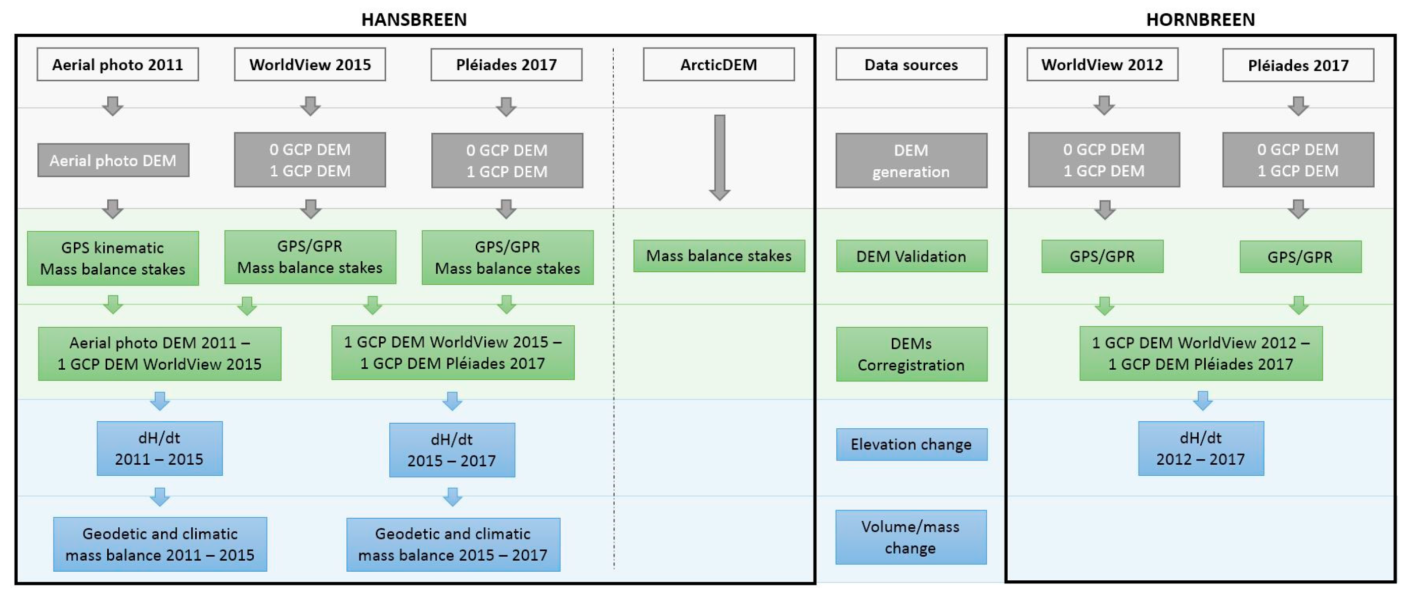
3. Datasets and Processing

In this study, we generated DEMs from different sources. Furthermore, we validated these DEMs, as well as individual strips of the ArcticDEM with in-situ data. In the end, we estimated geometry changes of Hansbreen and Hornbreen and compared the geodetic and climatic mass balance of Hansbreen. Figure 2 illustrates the flowchart of the data processing and result analysis.

3.1. DEM from Aerial Photographs

The aerial photo DEM was generated from 39 aerial photographs acquired by the Norwegian Polar Institute in 2011. The pixel size of the photographs equaled 0.5 m, and the average flight height was 7400 m a.s.l. Due to cloudiness over some areas, two sets of images were used: from 25.07.2011 and from 18.08.2011. To take into account surface elevation changes of the glacier between both acquisitions, the aerial photo DEM over the Hansbreen area from August was elevationally adjusted to July by removing the mean elevation difference estimated from the mass balance stake measurements.

The aerotriangulation (sigma0 = 5.7 μm) and DEM generation were carried out in INFO MATCH AT and INFO MATCH T software by MGGPAero (https://mggpaero.com). The 9 x,y,z GCPs measured with dGPS (differential Global Positioning System) and 20 z-points were used for aero-triangulation of the photographs. The RMSE of the GCP was: m_x = 0.19 m, m_y = 0.13 m, m_z = 0.02 m. The horizontal resolution of the aerial photo DEM was 5 m. The product was oversampled to 2 m resolution (bilinear interpolation), to compare it with other products used in this study. Considering results from Hansbreen in the ablation zone [31,32] and on Kongsvegen [33], glacier elevation changes due to emergence or submergence velocities are within range of precision of survey and might be neglected for such almost flat glaciers.

3.2. VHR DEM Generation

In this study we used two WorldView-2 Ortho Ready 2A stereo pairs and two Pléiades 1B stereo pairs (

Table 1. Characteristics of data used for DEM generation and reference data used for model validation. Reference data: Mass balance stakes—position of mass balance stakes measured by precise differential GPS (dGPS); dGPS_kinematic—dGPS positions recorded along profiling over the glacier; GPR/GPS—positions referred to in terms of elevation to previous summer surface derived from spring dGPS profiling and GPR survey for snow depth, taking into account compensation due to ablation between date of image acquisition and end of ablation period.

Glacier	DEM Source	Acquisition Date	Ref. Data	Dates of Ref. Data	Number of Ref. Points	Uncertainty Ref. Data (m)
Hansbreen	Aerial photographs	25.07.2011/ 18.08.2011	Mass balance stakes GPS_kinematic	27.07–28.08.2011 22–30.09.2011	13 19 980	0.2 0.5
	WorldView-2	21.08.2015	Mass balance stakes GPR/GPS	15–21.08.2015 18.04.2016	13 74 830	0.2 0.75
	Pléaides 1A	20.08.2017	Mass balance stakes GPR/GPS	17–23.08.2017 19.04.2018	13 83 356	0.2 0.75
Hornbreen	WorldView-2	15.08.2012	GPR/GPS	20.04.2013	9 721	0.75
	Pléaides 1B	02.08.2017	GPR/GPS	26.04.2018	28 932	0.75

, Figure 1). WorldView-2 launched 8 October 2009 has a 0.46 m horizontal resolution at nadir and 0.52 m off-nadir in the panchromatic band. In eight multispectral bands the resolution is 1.85 m at nadir and 2.07 m at 20° off-nadir (https://www.digitalglobe.com). More detail on the WorldView-2 system and its use in glaciology can be found in Fieber et al. [13] and at https://www.digitalglobe.com.

The Pléiades system consists of twin satellites: 1A (launched 17 December 2011) and 1B (launched 1 December 2012). The Pléiades horizontal resolution at nadir in panchromatic band is 0.7m, while in multispectral bands (blue, green, red and near-infrared) it is 2.8 m (https://pleiades.cnes.fr). However, the primary product used for DEM generation is oversampled and delivered at 0.5 m and 2 m resolution. The images of a Pléiades stereo pair are acquired along the orbit (along track) within a few tens of seconds [12], providing an homogeneous product [34]. More detail on the Pléiades system and its application in glaciology can be found in Berthier et al. [12], Rieg et al. [14] and Gleyzes et al. [35].

DEMs from WorldView-2 and Pléiades were processed using the Rational Function Model (RFM) developed in the OrthoEngine module of PCI Geomatica 2016. The RFM model, defined as a ratio of two cubic polynomials, is currently the most popular generic sensor model used in the field [36,37,38,39,40]. Both types of stereo pairs (WorldView-2 and Pléiades) contain the RPC files, which are used to define the initial functions for transforming the sensor geometry to image geometry [14]. This allowed us to generate DEMs without any GCP (0 GCP DEM). Since biases or errors still exist in the RPCs, the results can be improved with a polynomial adjustment and several accurate GCPs [34]. In our study, to improve image orientation, additional DEMs based on one GCP for each stereo pair (1 GCP DEM) were also created. Unfortunately, for both glaciers no more precisely measured GCP was available in a suitable spatial distribution, so we tested only zero-order RPC adjustment (https://support.pcigeomatics.com). To evaluate how the single GCP improved the results, two types of DEMs based on the RPCs-only (without any GCP) and GCP-enhanced RPC (using one GCP) were compared with the field data.

We generated the DEMs with a pixel size of 2 m. In addition to pixel size, two other main parameters can be tuned during DEM generation with OrthoEngine: the level of detail of the DEM (from low to very high) and the type of relief in the scene (from flat to mountainous) [12]. After testing preliminary results, we used the low level of detail and mountainous type of relief in the study.

3.3. ArcticDEM

The ArcticDEM is an open product provided by the Polar Geospatial Center [15]. It is an NGA–NSF (National Geospatial-Intelligence Agency and National Science Foundation) public–private initiative to automatically produce a high-resolution, high-quality, digital surface model of the Arctic using optical stereo imagery, high-performance computing, and open source photogrammetry software. ArcticDEM data is constructed from in-track and cross-track high-resolution (~0.5 m) imagery acquired mainly from the panchromatic bands of the WorldView-1, WorldView-2, and WorldView-3 satellites (https://www.pgc.umn.edu/data/arcticdem/).

In the study, we assessed the accuracy of five Strip ArcticDEM products (

Table 2. Strip ArcticDEM used in the study with horizontal (Dx, Dy) and vertical offset (Dz) from product metadata applied to DEMs. Mass balance stakes measurements (0.2 m uncertainty) were used as reference for DEMs validation.

ArcticDEM Date	Satellite	Dx (m)	Dy (m)	Dz (m)	Date Ref. Data	Ref. Points Number
20.04.2013	WV-1	–0.47	0.80	1.59	15.04.2013	18
13.07.2013	WV-2	0.62	–1.12	–0.19	07.07.2013–20.07.2013	20
14.03.2014	WV-1	2.86	–1.08	0.44	16.03.2014	5
10.07.2015	WV-3	–2.04	0.61	0.40	06.07.2015–12.07.2015	16
21.08.2015	WV-2	40.751	–23.655	19.654	15.08.2015–21.08.2015	21
17.09.2015	WV-2	16.995	3.724	–5.902	09.09.2015–17.09.2015	14

) provided at 2 m spatial resolution (v3.0 Pan-Arctic, RELEASE 7), as ~17 km wide and ~110 km long strips. The validation was done over the Hansbreen area, based on mass balance stake measurements. The Strip ArcticDEM files contain NASA ICESat altimetry offsets within the metadata, but these values are not applied to the provided DEM files. Here, we assess the Strip ArcticDEM product after applying these offsets (Table 2).

3.4. Validation Data

3.4.1. Mass Balance Stakes

The elevation accuracy of DEMs over Hansbreen was validated with static dGPS survey of mass balance stakes (Figure 3 and Figure 4), measured year-round every week in the ablation part and every month in the accumulation part. The stake positions and glacier surface height were measured with dGPS with ~0.05 m accuracy. The stake measurements mostly coincide with the dates of satellite images which were used for DEM generation (Table 1 and Table 2). However, we take into consideration the surface roughness around the stakes, so the final accuracy of the height measurement was assessed as 0.2 m.

3.4.2. GPR and GPS Kinematic Data

Apart from the mass balance stakes over Hansbreen, the elevation accuracy of DEMs over glacierized areas was validated with GPS kinematic data acquired in the field in September 2011 over Hansbreen and during spring GPR surveys over Hansbreen and Hornbreen (Table 1, Figure 3, Figure 4 and Figure 5). In order to take into account the difference between the date of the satellite imaging performed during the ablation period and the dates of spring GPR measurements after the ablation season, we subtracted the snow layer (known from the GPR measurements) from the spring surface positioned by GPS, and applied an ablation correction. Based on seven to nine ablation stakes on Hansbreen and meteorological data, the ablation correction has been determined as the linear relationship between ablation and altitude in the period from the date of satellite images to the end of the ablation period. The ablation correction ranged from 0.5 m in 2015 and 1.15 m in 2017 at the glacier front to no ablation in the highest accumulation zones (with an accuracy of ±0.05 m). In 2011, due to gaps in the ablation stakes data, we used ultrasonic distance meters (SR50) located at two altitudes (187 and 424 m a.s.l.) to estimate the ablation correction as 0.6 m to 1.9 m (±0.1 m). The correction for emergence or submergence velocity has been neglected as based on observations in Hansbreen frontal area [31,32] and on Kongsvegen [33,41] changes in elevation can be approximated by the specific mass balance. Finally we have obtained summer surface elevation along spring GPR profiles.

Uncertainty assessment of summer surface glacier elevation (${\epsilon }_S$) derived from next spring GPR/GPS survey is expressed as:

$${\epsilon }_S=\sqrt{{\epsilon }_{GPR}{}^2+{\epsilon }_H{}^2+{\epsilon }_a{}^2}$$

(1)

where ${\epsilon }_{GPR}$ is the error of snow depth derived from GPR, ${\epsilon }_H$ is the error of dGPS vertical position of GPR survey assumed as 0.5 m on average, and ${\epsilon }_a$ is the error of ablation compensation.

The snow thickness error (${\epsilon }_{GPR}$) has been estimated similarly to the ice thickness error computation method as proposed by Lapazaran et al. [42].

$${\epsilon }_{GPR}=\sqrt{{\left({\epsilon }_c\frac{\tau }{2}\right)}^2+{\left(c\frac{{\epsilon }_{\tau }}{2}\right)}^2}$$

(2)

where ${\epsilon }_c$ is radio-wave velocity (RWV) error, ε_τ is two-way travel time (TWTT) error, c is RWV in snow, and τ is TWTT to the previous summer surface.

The RWV error (${\epsilon }_c$) is assumed to be not larger than 5% of the applied constant velocity in glacier snowpack of 0.21 m ns⁻¹ [43]. The error in travel time (ε_τ) through the snow cover to the previous summer surface can be identified with vertical accuracy, assumed as the inverse of the dominant frequency of GPR [42]. Applying in the snow survey the 800 MHz central frequency antenna, the ε_τ is 1.25 ns. Assuming RWV in snow of 0.21 m ns⁻¹, the wavelength (λ) is 0.2625, and consequently in terms of depth ε_τ is 0.131 m. The overall ${\epsilon }_{GPR}$ increases with snow depth. In particular areas and seasons, its average values are as follows: Hansbreen 2016: 0.16 m (SD: 0.02 m), Hansbreen 2018: 0.17 m (SD: 0.02 m), Hornbreen 2013: 0.16 m (SD: 0.01 m) and Hornbreen 2018: 0.18 m (SD: 0.01 m).

The error of ablation compensation (${\epsilon }_a$) comprises elevation determination errors of both spring kinematic GPS error (${\epsilon }_H$= 0.5m) and summer dGPS error of stake positions (${\epsilon }_{HA}$= 0.2m), and the square root of the sum of squares is equal to 0.54 m. The average error of determination of summer surface elevation ${\epsilon }_S$ from GPS/GPR data (Table 1) considering all components discussed above is 0.75 m.

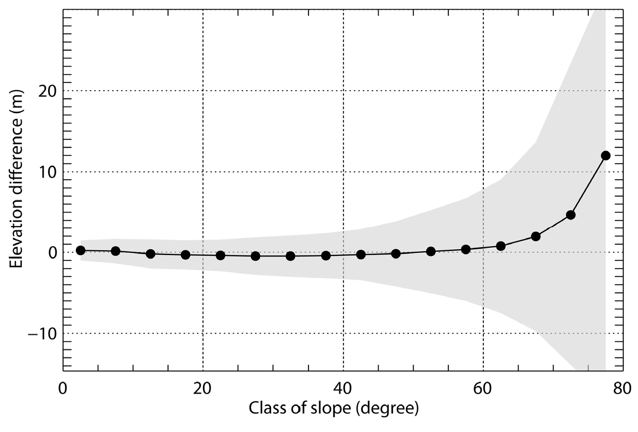
3.5. Quality Measures of DEMs

The quality of the DEMs was characterized by different statistical measures: (i) median, to evaluate the vertical accuracy of the DEMs, and (ii) standard deviation (SD) and normalised median absolute deviation (NMAD) to characterize their vertical precision, following Berthier et al. [12] and Hobi and Ginzler [44]. Additionally, maximal error is shown here. The NMAD is a measure of the dispersion of the data that is less sensitive to outliers than the standard deviation [45] and is defined as:

NMAD = 1.4826 · median (│Δh_j − mΔh│)

(3)

where Δh_j denotes the individual errors and mΔh is the median of the errors.

We assessed here the vertical quality of the DEMs without any horizontal and vertical DEM shifting. Assessment of the horizontal DEM accuracy was not possible given the lack of a GCP measured with decimal accuracy on the stable terrain and recognizable on satellite images. This would enable users who are not in possession of many GCP and any field data to determine approximate DEM quality.

3.6. DEM Co-Registration

To investigate glacier surface elevation changes, WorldView and Pleiades DEMs generated with 1 GCP for each study site were co-registered using the method described by Berthier et al. [46]. The difference between the two DEMs was then computed pixel-by-pixel on the ice-free areas. The precision of the elevation difference map was also assessed over the stable terrain, taking into consideration the slope of the terrain.

3.7. Geodetic Mass Balance

The total geodetic mass balance (B_geod) of Hansbreen was estimated similarly to Deschamps-Berger et al. [4], as the sum of the mass change by surface elevation changes over the glacierized area (dV/dt) and by change in the terminus position (q_t):

$$B_{geod}=\frac{\Delta V}{\Delta t}+q_t=\Delta H_1·A_1+\Delta H_2·A_2$$

(4)

where $\frac{\Delta V}{\Delta t}$ is volume change in function of time defined as difference between DEMs ($\Delta H_1$) multiplied by glacier area ($A_1$). Change in the terminus position ($q_t$) is defined as difference between DEMs ($\Delta H_2$) multipled by glacier area recession ($A_2$). Component $q_t$ includes recession of glacier front terminated in water and over the land. The error was estimated using the total differential function, as follows:

$$\sigma B_{geod}{}^2=\sigma {\left(\frac{\Delta V}{\Delta t}\right)}^2+\sigma {\left(q_t\right)}^2=\delta \Delta H_1{}^2·A_1{}^2+\delta A_1{}^2·\Delta H_1{}^2+\delta \Delta H_2{}^2·A_2{}^2+\delta A_2{}^2·\Delta H_2{}^2.$$

(5)

where the accuracy of DEM vertical changes ($\delta \Delta H_1$, $\delta \Delta H_2$) was calculated for each period based on

Table 3. Vertical quality of the DEMs estimated from field measurements for both studied glaciers. Two types of DEMs from satellites WorldView-2 and Pléiades images are presented: generated without any GCP (ground control point) and with one GCP located in stable terrain. All statistics are determined over the glacierized area. The amount and uncertainty of the reference data used for statistics are listed in Table 1.

Glacier	VHR System	No of GCP	Ref. Data	Median (m)	SD (m)	NMAD (m)	Max Error (m)
Hansbreen	Aerial photographs 2011	9 xyz 20 z	Mass balance stakes GPS-kinematic	−0.23 −0.55	0.60 0.52	0.72 0.43	−1.76 5.14
	WorldView-2 2015	0	Mass balance stakes GPR/GPS	0.10 0.80	0.19 1.07	0.28 0.57	0.35 13.16
		1	Mass balance stakes GPR/GPS	−0.45 0.35	0.18 0.98	0.21 0.50	−0.82 12.06
	Pléaides 1A 2017	0	Mass balance stakes GPR/GPS	7.54 8.48	1.52 2.64	1.39 1.83	8.65 23.64
		1	Mass balance stakes GPR/GPS	−0.36 0.57	0.24 0.54	0.19 0.44	−0.81 9.39
Hornbreen –Flatbreen	WorldView-2 2012	0	GPR/GPS	0.26	1.18	1.2	4.06
		1	GPR/GPS	0.53	0.63	0.7	2.62
	Pléaides 1B 2017	0	GPR/GPS	2.91	1.94	1.68	19.65
		1	GPR/GPS	0.66	0.49	0.38	3.07

. Area accuracy ($\delta A_1,\delta A_2$) was estimated as the accuracy of surface calculation based on the methodology for calculating an area in ArcGIS.

The volume changes (dV/dt) of Hansbreen were derived from differential DEMs, i.e. the summation of the elevation-change pixels over the glacier surface multiplied by the pixel area [47]. The volume changes were estimated to the minimal front positions in the studied period, i.e. 2015 for period I (2011–2015) and 2017 for period II (2015–2017). Shadowed areas were removed from analyses. The missing parts represent 9% of Hansbreen.

Converting volume change to mass change in water equivalent (w.e.) (and the converse) requires knowledge of the effective density, typically assuming all elevation changes consist of changes in ice thickness ρ = 850 to 900 kg m⁻³ [4,47,48]. In our calculation we assumed the ice density to be ρ = 900 kg m⁻³ below the average firn line and ρ = 600 kg m⁻³ above the firn line. These values are consistent with the densities measured in situ [32] and used to calculate the Hansbreen mass balance reported in WGMS (https://wgms.ch/). The average firn line for each study period was estimated from radar satellite data (Sentinel-1, Alos-2 Palsar and Radarsat-2) with ISO and H-alfa-Wishart classifications [49] and validated with GPR data.

The volume of ice loss by frontal recession (q_t) was estimated from the bathymetry from Błaszczyk et al. [29], the glacier surface elevation at the beginning of the period and the area of recession from the adequate orthoimages. The component of the retreated front area was converted to mass using ice density ρ = 900 kg m⁻³. The error for the bedrock elevation is ~10 m.

The DEMs from 2012 for Hornbreen do not cover the glacier fully, so we could not analyze the large part of the glacier accumulation zone. Therefore, we only describe the surface elevation changes over the area overlapped by two DEMs. Shadowed areas covering 3% of the Hornbreen area were removed from the further analyses.

3.8. Climatic Mass Balance

The total mass balance of tidewater glaciers has two components [50]: the climatic–basal balance (B) and the frontal ablation (A_f). The climatic–basal balance (B) is the sum of the surface mass balance (B_sfc), the internal mass balance (B_i) and basal balance (B_b). The B_i includes internal ablation and internal accumulation below summer surface and was estimated as 0.04 m w.e. on Hansbreen in 2007/2008 [32]. Thanks to applying the end of summer snow density 6–17% of B_i is included in surface mass balance measurements on Hansbreen [32]. However, the B_i in firn from previous seasons has been neglected. The B_b in Svalbard glaciers has been not measured directly, but according to Cuffey & Paterson [51] basal melting underneath temperate ice of moderate sliding rate can be in the order of a few millimeters w.e., whereas accretion may locally take place in overdeepenings. As B_b values are in range of mass balance measurements errors we consider them as negligible.

In order to achieve results which would allow us to compare it to the geodetic mass balance, our study focuses on total climatic mass balance (M_clim) defined as the sum of surface mass balance (B_sfc) and frontal ablation (A_f):

$$M_{clim}=B_{sfc}+A_f=B_{sfc}+q_t+q_{fg}=B_{sfc}+\Delta H_2·A_2+H·w·v$$

(6)

where $B_{sfc}$ is surface mass balance calculated as linear regression of elevation and net mass balance from WGMS data and $A_f$ is total frontal ablation defined as sum of glacier retreat ($q_t$) and glacier ice flux ($q_{fg}$) [29,52]. H is the ice thickness along the flux gate, w is the width of the flux gate, and v is the velocity across the flux gate. The estimation of q_t is described in Section 3.6. The ice flux through a flux gate near the calving front (q_fg) used in this study was estimated by Błaszczyk et al. [29] based on the TerraSAR-X velocity data from 2012.

The error was estimated using the total differential function, as follows:

$$\sigma M_{clim}{}^2=\sigma B_{sfc}{}^2+\sigma q_t{}^2+\sigma q_{fg}{}^2$$

(7)

$$\sigma B_{sfc}=a_{20xx}·{\delta }_{DEM}$$

(8)

$$\sigma q_t{}^2=\delta \Delta H_2{}^2·a_2{}^2+\delta a_2{}^2·\Delta H_2{}^2$$

(9)

$$\sigma q_{fg}{}^2=w^2·v^2·\delta H^2+H^2·w^2·\delta v^2+H^2·v^2·\delta w^2$$

(10)

where ${\delta }_{DEM},\delta H^2,\delta v^2,\delta w^2$ is the accuracy of each of the variables described above, and a_20xx is the slope coefficient from linear functions used to calculate the surface mass balance for each year (2011–2017).

To estimate the surface mass balance $B_{sfc}$ we used data of summer, winter and net mass balance of Hansbreen from WGMS and the Institute of Geophysics, Polish Academy of Sciences. Based on DEMs and using the year-to-year relationship between net mass balance and elevation, surface mass balance has been calculated for each season and summarized to the analyzed period. Conversion from water equivalent to volume changes was based on the same principles as in Section 3.7. In the calculation we neglected the 2013 data from Hansbreen as unreliable, and use available mass balance data from Werenskioldbreen, a land-based glacier located next to Hansbreen. Similarly to geodetic volume changes, surface mass balance was estimated to the minimal front positions in the study period.

4. Results I: DEMs Quality

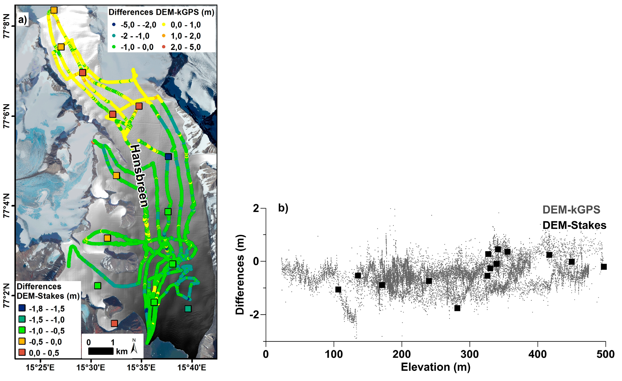
4.1. DEM from Aerial Photographs

Figure 3 and Table 3 summarize the results of the evaluation of the aerial photo DEM with stakes and kinematic GPS measurements. The vertical accuracy (median elevation difference) is higher for mass balance stakes than for GPS measurements. While the vertical precision (NMAD and SD) is lower for mass balance stakes than for GPS measurements. Overall, the accuracy of this DEM is within the 1 m. However, the aerial photo DEM also has parts with errors over 1 m.

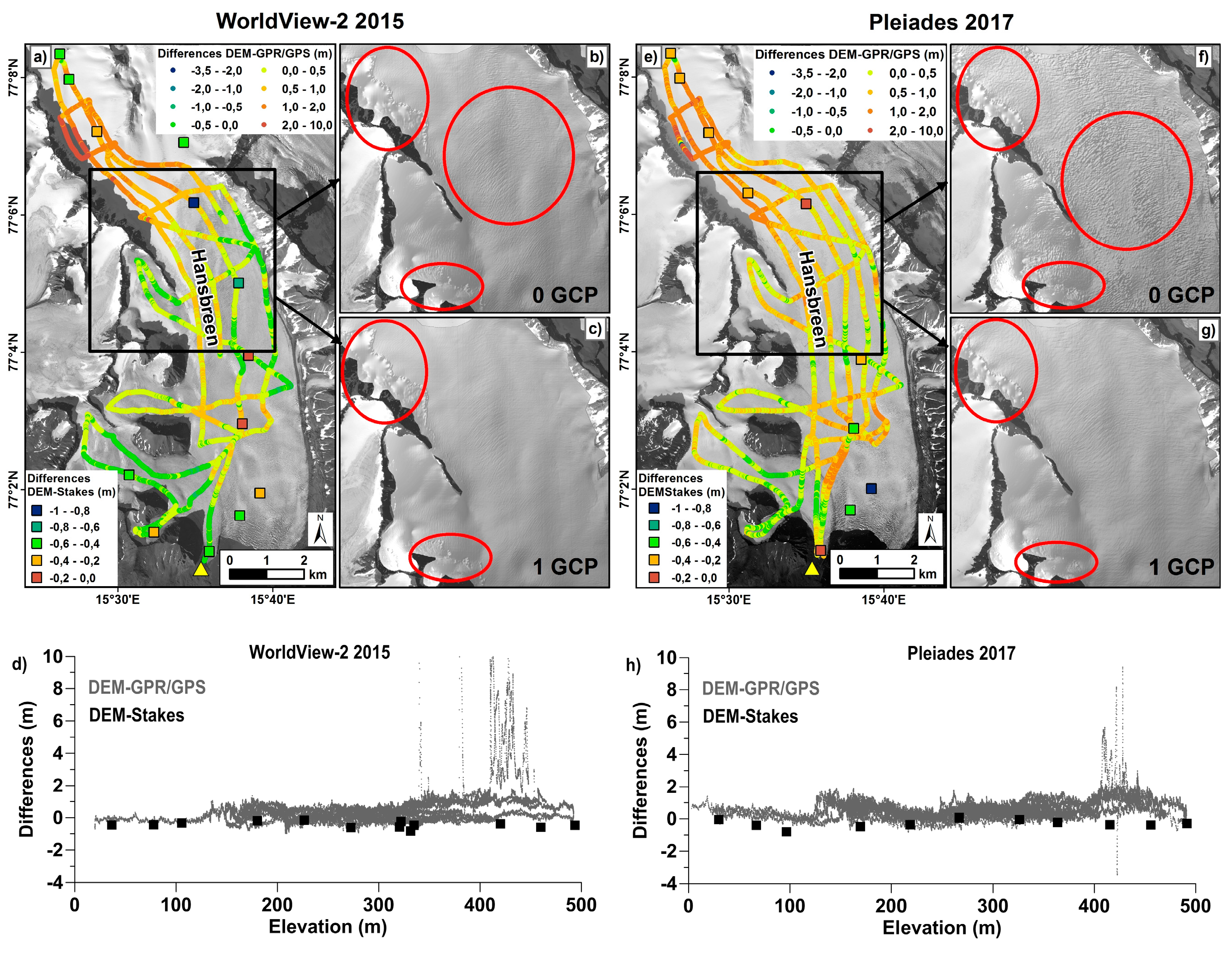
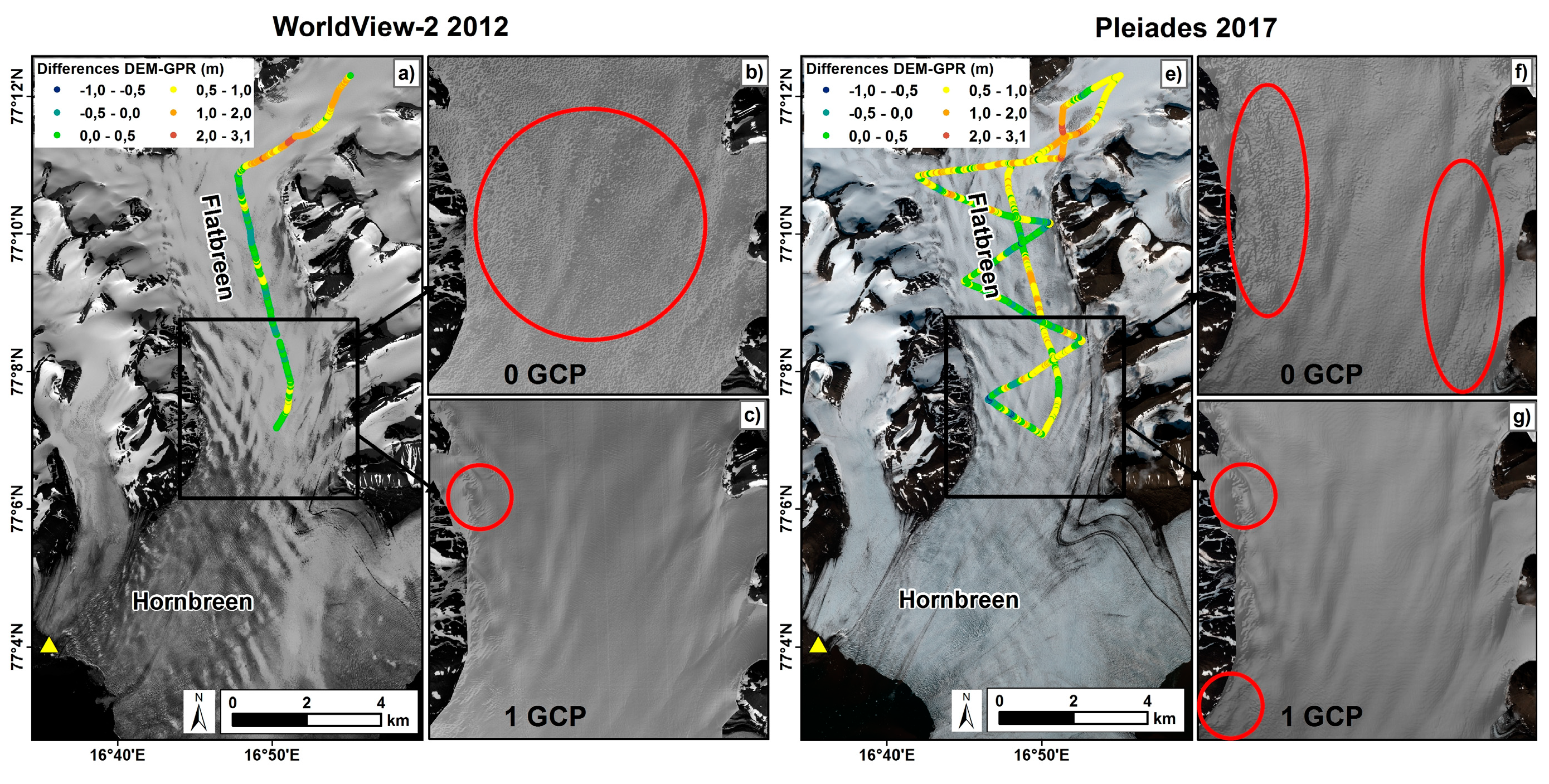
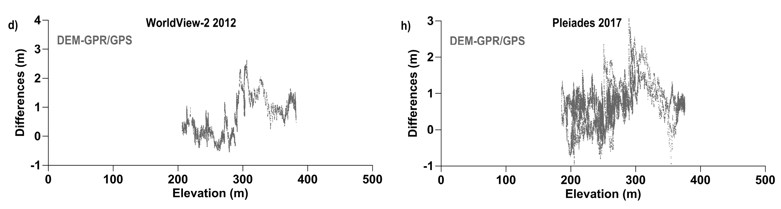
4.2. DEM from Pléiades and WorldView-2

The quality of DEMs generated using one GCP and without GCPs was examined based on two reference datasets for Hansbreen (stake position measurements and GPR/GPS data) and only GPR/GPS data for Hornbreen (Figure 4 and Figure 5, Table 3).

The quality of 0 GCP DEM and 1 GCP DEM generated from WorldView-2 stereo pairs over both glaciers is comparable (Table 3). Median and maximal errors estimated for mass balance stakes on Hansbreen are generally better in the case of the DEM generated without using a GCP, while precision (NMAD and SD) is better for 1 GCP DEM. Statistical measures for GPR/GPS data on both glaciers show a slightly better precision of 1 GCP DEM (e.g., NMAD below 0.5 for Hansbreen and 0.7 m for Hornbreen), but accuracy (i.e. the median of the elevation differences) for Hansbreen is better for 1 GCP DEM, whilst for Hornbreen for 0 GCP DEM. However, the differences are within the accuracy limits of the reference data. All DEMs from WorldView-2 have a very good accuracy (median < 1 m) and precision (NMAD < 1.2 m) over the glacierized area, but considering all results, the use of 1 GCP generally improves DEM accuracy.

In the case of Pléiades stereo pairs, all the statistics indicate that using just one GCP considerably improves the DEM quality. The vertical bias (i.e. median) evaluated from GPR/GPS data and mass balance stakes decreased from a few meters for 0 GCP DEM to values below 0.7 m in case of 1 GCP DEM. Precision (e.g., NMAD) over both glaciers ranged from 1.39 m to 1.83 m for 0 GCP DEM and from 0.19 m to 0.44 m for 1 GCP DEM.

Hillshades from the DEMs were generated for visual verification. Results show that DEMs generated without any GCP (Figure 4b,f and Figure 5b,f) are very coarse, while using just one GCP (Figure 4c,g and Figure 5c,g) significantly improves the DEM quality and makes the glacier surface much smoother. Given the presence of crevasses and natural ridges, artefacts are expected on the glacier surface. But detailed inspection and comparison of DEMs with orthoimages revealed that only 0 GCP DEM from WorldView-2 for Hansbreen (Figure 4b) represent the crevasses pattern adequately. The other 0 GCP DEMs are more chaotic and the artefacts do not reflect the glacier surface. Furthermore, both types of DEMs show large errors in areas affected by shadows of very steep mountains and low image contrast. Therefore, the values of statistics estimated from GPR/GPS data are higher than from mass balance stakes, as they present the DEM quality over a larger glacier area including these artifacts. Also, the error is higher in upper parts of the glaciers, due to difficulties in image correlation associated with low image contrast over shadowed and snow-covered areas (Figure 4 and Figure 5).

4.3. Quality of ArcticDEM Strips

Table 4. Vertical quality measures of the ArcticDEM (Strip DEM product) after applying horizontal and vertical offset presented in Table 2. All statistics are determined over the glacierized area.

ArcticDEM Date	Median (m)	SD (m)	NMAD (m)	Max Error (m)
20.04.2013	–0.36	0.53	0.25	–1.80
13.07.2013	3.97	0.65	0.69	5.84
14.03.2014	0.28	0.35	0.62	0.74
10.07.2015	1.69	0.63	0.54	2.19
21.08.2015	–67.15	1.56	1.51	–70.20
17.09.2015	–0.73	0.91	0.88	–3.20

summarizes the results of the evaluation of the quality of the Strip DEM product of ArcticDEM with mass balance stakes. Generally, the product after applying offset provided in metadata has good accuracy (median < 4 m) and precision (NMAD < 1 m) over the glacierized area. However, one product, the DEM from 21.08.2015, exhibits a gross height error (median over −67 m). The WV-2 stereo pair used for this particular DEM is the same as the one we used to generate the surface model over Hansbreen (Table 1). From detailed analyses we concluded that the offset provided in metadata with Strip ArcticDEM was wrong. But the vertical accuracy of ArcticDEM strips without applying the coefficient was still very low (the median was c. −46.5 m) while precision increased (NMAD equaled 0.25 m). That allows us to deduce that the analyzed DEM was probably incorrectly georeferenced.

4.4. DEM Co-Registration

The difference between the two DEMs computed on the ice-free areas is presented in

Table 5. Horizontal and vertical shifts of the slave DEM in relation to the master DEM calculated during the co-registration process over the stable terrain. For Hansbreen, we also provide the residual of the triangulation which quantifies the consistency of our 3D co-registration. We also provide the NMAD of the elevation difference over the stable terrain with a slope of less than 10°, a range of slope similar to the glacier terrain.

Acquisition	Shift E/W (m)	Shift N/S (m)	Shift Vertical (m)	NMAD Slopes < 10°
A - Hansbreen 2015–2011	1.00	1.31	−0.52	1.39
B - Hansbreen 2017–2015	−1.14	−1.52	0.29	0.48
C - Hansbreen 2017–2011	0.44	0.14	0.04	1.41
Residual (C − (A + B))	0.58	0.35	0.27
Hornbreen 2017–2012	2.85	−0.94	−1.40	1.48

. We also estimated the residual of the triangulated shift vectors for Hansbreen (between 0.27 m and 0.58 m in the X,Y,Z directions), which is the remaining un-removed shift between the three datasets and thus represents the internal consistency of the datasets [10]. For all DEM differences (only one is shown in Figure 6), there is a strong relationship between the dispersion of the residuals (NMAD) and the slope of the terrain, a feature observed in earlier studies using VHR stereo-images [23,53]. The precision is high and more or less constant for slopes below 40 to 50° and then the NMAD increase drastically. If we restrict the analysis to a range of slope similar to the one found on the glacier surface (<10°) we find dispersion of the elevation difference (last column of Table 5) which is in agreement with the results of the evaluation off the glacier. It suggests that the stable terrain can be used to assess the precision of the elevation difference on glaciers, [21] if the difference of slopes is accounted for.

5. Results II: Glaciological Interpretation

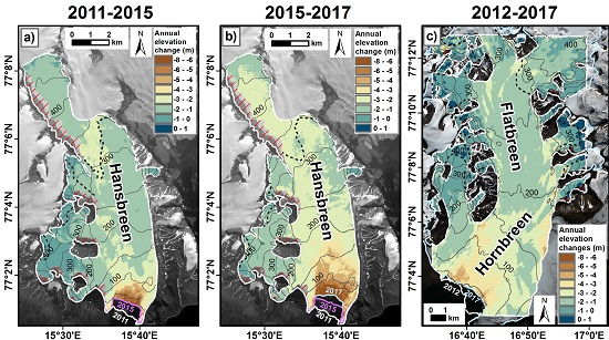
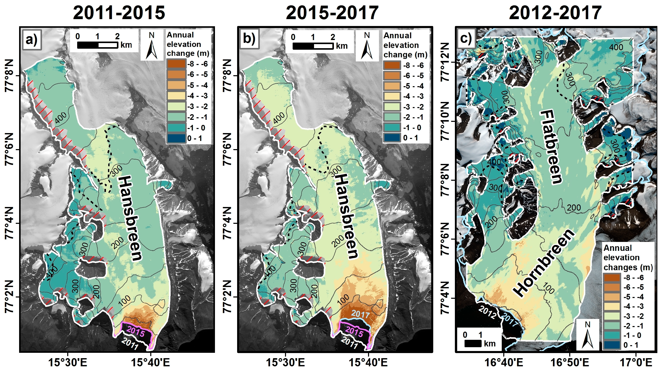
5.1. Geometry Changes of Hansbreen

The total and annual elevation changes for Hansbreen during period I (2011–2015) and period II (2015–2017) are shown in Figure 7, Figure 8 and

Table 6. The total and mean annual rate of: volume change (dV/dt), retreat mass (q_t), discharge at the terminus (q_fg), surface mass balance (B_sfc), geodetic mass balance (B_geod) and climatic mass balance (M_clim) of Hansbreen. Annual ice flux near the calving front (q_fg=0.271 km³ a⁻¹) based on the TerraSAR-X velocity data from 2012 is calculated in Błaszczyk et al. [29] and multiplied by the number of years. Note that 9% of the Hansbreen area is missed in estimations, due to shadows.

		dV/dt	qt	qfg	Bsfc	Bgeod	Mclim
2011–2015	Total change (km3)	−0.327 ± 0.076	−0.090 ± 0.010	−0.108 ± 0.030	−0.174 ± 0.004	−0.417 ± 0.077	−0.373 ± 0.032
	Annual change (km3 a−1)	−0.082 ± 0.019	−0.023 ± 0.002	−0.027 ± 0.008	−0.043 ± 0.001	−0.104 ± 0.019	−0.093 ± 0.008
	Specific mass balance (m w.e. a−1)	−1.43 ± 0.33	−0.43 ± 0.05	−0.51 ± 0.14	−0.82 ± 0.02	−1.86 ± 0.33	−1.76 ± 0.16
2015–2017	Total change (km3)	−0.227 ± 0.099	−0.052 ± 0.005	−0.054 ± 0.015	−0.112 ± 0.002	−0.279 ± 0.099	−0.218 ± 0.016
	Annual change (km3 a−1)	−0.113 ± 0.050	−0.026 ± 0.002	−0.027± 0.008	−0.056 ± 0.001	−0.139 ± 0.050	−0.109 ± 0.008
	Specific mass balance (m w.e. a−1)	−2.04 ± 0.90	−0.49 ± 0.04	−0.52 ± 0.14	−1.06 ± 0.02	−2.53 ± 0.91	−2.07 ± 0.14

. Surface elevation changes of Hansbreen were negative over the whole area. The mean annual elevation changes were more negative in period II (−2.4 m a⁻¹) than in period I (−1.7 m a⁻¹). The thinning rate in the lowest parts of the glacier increased from 7 m a⁻¹ in period I to 10 m a⁻¹ in period II. Asymmetrical mass loss on the main stream of Hansbreen is also visible [32]. Ice loss was noted to be greater in the western part of its main trunk (Figure 7).

The annual volume of ice loss by Hansbreen (dV/dt; Table 6) was higher in period II (−0.113 ± 0.050 km³ a⁻¹) than in period I (−0.082 ± 0.019 km³ a⁻¹). This is in accordance with the location of the average firn line, which is higher in the second period. Note, however, that shadowed areas were removed from the estimations (see above) and the total glacier volume change in both periods was probably slightly more negative.

Apart from the surface lowering, the Hansbreen front also retreated considerably (Figure 7). The glacier lost about 2.1% and 1.1% of its area in periods I and II, respectively. To account for the retreat of the glacier front, we estimated the volume of ice loss over the retreat area (q_t ). Similar to the surface thinning, the mass loss by Hansbreen due to retreat was greater in period II (−0.026 ± 0.002 km³ a⁻¹) than in period I (−0.023 ± 0.002 km³ a⁻¹). Taking all the components into account, both total geodetic and climatic mass balance are more negative in the second than in the first period.

5.2. Geodetic and Climatic Mass Balance of Hansbreen

Both geodetic and climatic mass balance of Hansbreen were more negative in period II than in period I (Table 6). Furthermore, the climatic mass balance in both study periods is underestimated, compared with the geodetic data. In period I the difference makes up ~11% of the geodetic mass balance, whilst in period II the residual is even higher, ~22%. The total geodetic mass loss in period I, including terminus position change, can be divided into ~78% due to volume change and 22% due to retreat of the terminus position. In period II, the values are ~81% and 19%, respectively. Taking the glacier volume 9.6 km³ [24], the total geodetic mass loss in the whole study period 2011–2017, including terminus position change, represents ~7% of the total glacier volume.

5.3. Geometry Changes of Hornbreen

Since the 2012 DEM does not cover the whole area of Hornbreen we can only draw general conclusions about the glacier (Figure 7 and Figure 8). Surface elevation changes were negative over the main trunk of the Hornbreen–Flatbreen system. However, in contrast to Hansbreen, we noted an elevation increase in the parts of the tributary glaciers feeding the main part of Hornbreen (above ~400 m a.s.l.). Lack of data prevents us from drawing conclusions about the higher parts of the main trunk of the glacier.

The average annual elevation changes over the studied area amounted to −1.6 m a⁻¹ and in the lowest parts of the glacier surface lowering occurred at a rate of −6 m a⁻¹. The Hornbreen front also retreated considerably (Figure 7). The glacier lost about 2.1% of its area in the period 2012–2017.

6. Discussion

6.1. Quality of DEM Based on the Aerial Photographs

The aerial photo 2011 DEM was made from photographs taken during two flights over three weeks apart. Although the DEM over the Hansbreen area was elevationally adjusted, merging lines are visible on the final DEM. Nevertheless, the final accuracy of the DEM allowed us to use the model to estimate the geodetic mass balance. The vertical bias (median) on precisely measured mass balance stakes (−0.23 m) and median of kinematic GPS (−0.55 m) were within the accuracy of the measurements. NMAD on mass balance stakes equaled 0.72 m, whilst NMAD of kinematic GPS (0.43 m) was within the accuracy of the measurements. This accuracy is better than that of the DEMs produced in the northern part of Svalbard by the Norwegian Polar Institute [3], which are characterized by a stated accuracy of ~2 to 5 m. However, we did not evaluate the accuracy of our DEM 2011 outside glaciers, where the accuracy is likely to differ, depending on the terrain type.

6.2. Quality of DEMs Based on Pléiades and WorldView-2 with and Without the Use of GCPs

The comparison of DEMs processed from Pléiades and WorldView-2 based only on RPC files, without the use of GCPs, shows better accuracy and precision of the DEMs from WorldView-2. The average median and NMAD for all WorldView 0 GCP DEMs is 0.39 m and 0.68 m, respectively, whilst for all Pléiades 0 GCP DEMs median and NMAD equals 6.31 m and 1.63 m. Using one GCP substantially improved vertical quality. Average median and NMAD for both WorldView 1 GCP DEMs is 0.14 m and 0.47 m, respectively, whilst for Pléiades 1 GCP DEMs it equals 0.29 m and 0.34 m, respectively.

Although the accuracy of 0 GCP DEM and 1 GCP DEM generated from WorldView-2 is very good, we advise using at least one GCP. According to Choi et al. [54], the accuracy of stereo models substantially improves with just one GCP, and when more GCPs were used the accuracy increased slightly (e.g., [37,44]). Also, visual inspection of DEMs revealed that using just one GCP considerably improved the final product.

The lower accuracy of 0 GCP DEM for the Pléiades constellation is in agreement with Rieg et al. [14] who reported that GCPs substantially improved the vertical accuracy of DEMs calculated from Pléiades tri-stereo images. Also Berthier et al. [12] found that the vertical biases of the Pléiades DEMs were less than 1 m if GCPs were used, but reached up to 7 m without GCPs. Correspondingly, according to Cheng [34], it is possible to achieve accuracy of 1 m with GCP, and 10 m without GCP using PCI Geomatica software.

The tested methods show acceptable quality for estimating the geodetic mass balance budget of larger tidewater glaciers in Svalbard over relatively short periods of time. The average median and NMAD for all DEMs generated with 1 GCP equaled 0.22 m and 0.40 m, respectively. Regardless of the number of GCPs used, the horizontal and vertical shifts should be applied to DEMs [10,12,46] before performing elevation and volume change studies. The elevation difference between these DEMs off the glacier shows small residuals for gently sloping terrain and a much larger dispersion for slopes larger than 40–50°. Accuracy assessment should thus be performed on a range of slopes off glacier similar to the type of slopes found on the glacier.

Two general problems of optical remote sensing data are the shadows due to mountains, and fresh snow over glaciers [1,10,14]. Visual inspection of hillshaded DEMs revealed that using just one GCP considerably improves the surface model. However, the DEMs in shadow-affected or snow-covered areas exhibited lower accuracy, i.e. average bias was 1 m for Hornbreen and 1.5 m for Hansbreen, but maximal residuals reached even 10 m on Hansbreen (see Figure 4d,h and Figure 5d,h).

In the quality assessment of the DEMs over glaciers we used GPR/GPS data characterized by relatively low accuracy. The GPR/GPS data refers to the last end-of-summer surface and had to be corrected by melting between the image acquisition date and the end of the ablation season. Additionally, sub-snow spring surface elevation may differ from last summer surface due to the vertical component of glacier movement, which was not implemented in the correction procedure. Nevertheless, we found the data highly valuable, as it helped us to validate the DEM accuracy in white, featureless areas above the transient snow line and in the shadow areas. In particular, the GPR/GPS data enabled us to determine the approximate accuracy for Hornbreen, where we have no other in situ data.

6.3. Quality of the ArcticDEM Strips

According to the provider, the absolute accuracy of the Strip DEM product of ArcticDEM generated without GCPs is approximately 4 m in the horizontal and vertical planes (https://www.vedur.is/media/frettir/ArcticDEM_Documentation_and_User-Guidance_Rel4.pdf). The ICESat altimetry offsets provided within the metadata can be used to improve the product. These ICESat data points are filtered to exclude points in areas of high relief and over hydrographic features. But the documentation does not specify the accuracy of Strip DEM after applying the ICESat altimetry offsets and whether the points over glacierized area are excluded. ArcticDEM data is generated by applying stereo auto-correlation techniques using the SETSM software developed by Noh and Howat [22]. Automation and high-performance computing make it possible to generate a large amount of terrain in a short period of time (https://www.pgc.umn.edu/guides/arcticdem/introduction-to-arcticdem/). However, as shown in Table 4, automation can be also the source of gross errors. Here we found that the accuracy of the five Strip ArcticDEMs was better than 4 m and the precision larger than 1 m, but the mean bias of one DEM reached over 60 m. Thus, the final product should always be carefully controlled. Therefore, similarly to independently produced DEMs, horizontal and vertical shifts and co-registration should be applied to Strip ArcticDEM products [10,12,46] before performing any multitemporal studies.

6.4. Geometry Changes of Hansbreen and Hornbreen

The DEMs used in the study were collected from different time frame. Furthermore, the 2012 DEM for Hornbreen do not cover the whole glacier. That constrict direct comparison of the volume changes for both glaciers. These deficiencies are caused by lack of accessibility of cloud free images for the studied glaciers. However, comparing the elevation changes over the same altitude for Hansbreen and Hornbreen (Figure 8), we noticed a higher thinning rate for Hansbreen. We also noted higher retreat rate and surface lowering at the terminus of Hansbreen than on Hornbreen.

This study revealed a significantly faster thinning rate in the western Hansbreen area than in the eastern one. This pattern of glacier geometry changes is in opposition to the well-recognized asymmetry in snow distribution with prevailing snow deposition in the western bank of the glacier [28,32,43,55]. According to Grabiec [32], as winter snow accumulation does not drive the surface lowering, the asymmetric pattern of geometry changes can be explained by the spatial variability of both summer balance and glacier dynamics.

The mean elevation change of Hansbreen in the whole period 2011–2017 (−2 m a⁻¹) and Hornbreen in the period 2012–2017 (−1.6 m a⁻¹) is higher than previous results for Wedel Jarlsberg Land. The geodetic balance for Wedel Jarlsberg Land was estimated as −0.43 m a⁻¹ for the period 1936–1990 [1], and −0.65 m a⁻¹ in period 1990–2003/2007 [2]. Assuming an ice density 900 kg m⁻³ and 917 kg m⁻³ used by authors, respectively, the mean elevation change for Wedel Jarlsberg Land equaled 0.47 m a⁻¹ and 0.71 m a⁻¹. Bamber et al. [56] estimated lower average rates of thinning (−0.47 m a⁻¹) of four glaciers in southern Spitsbergen over the period 1996–2002. This comparison suggests that geodetic mass loss for glaciers in southern Spitsbergen has increased significantly in the last decade. Furthermore, the mean annual volume of ice loss by terminus retreat of Hansbreen for the entire study period 2011–2017 (0.024 km³ a⁻¹) is much higher than the estimate of 0.008 km³ a⁻¹ for the period 2006–2015 [29]. The difference is caused by a threefold increased retreat rate compared to the previous period.

Overall, we found that the rate of mass loss from the studied glaciers increased due to negative surface mass balance and faster retreat of glaciers fronts. As we do not have recent velocity data, we cannot attribute this to larger ice flux to the front (q_fg). Drawing general conclusions about the behaviour of glaciers in southern Spitsbergen based on data from only two tidewater glaciers over few seasons may raise some doubts. Nevertheless, the results are consistent with other studies indicating accelerated contributions of glaciers to sea level rise over recent decades due to surface lowering and/or increased glacier retreat and frontal ablation over the Arctic [26,57,58,59,60,61]. This is also consistent with the atmospheric warming reported across the Arctic during the 2000s [60,62].

6.5. Closing a Mass Budget of Hansbreen

Closing a mass budget relies on the absolute value of the mass budget components and on the associated error. With sufficiently large error bars, it would always be possible to close the mass budget [4]. In our study the geodetic mass balance of Hansbreen is more negative than the climatic mass balance, although the differences are within the error estimates. One explanation for the difference would be underestimation of the ice flux component, which was derived from Błaszczyk et al. [29] and estimated based on the TerraSAR-X velocity data from 2012 validated with annual GPS measurements. But the front velocities could have been higher in the recent period. This explanation would be in agreement with temperatures in Hornsund (https://monitoring-hornsund.igf.edu.pl). The average annual and summer (JJAS) temperatures in the period 2011–2017 were −1.6°C and 4.3°C respectively, whilst in 2012 annual temperature was higher (−1.1 °C) but summer temperatures were lower (3.6°C). Higher summer temperature after 2012 would cause more intense melting and faster flow of Hansbreen, as glacier velocity is mostly controlled by the distribution and pressure of water at the glacier bed [63,64,65], which facilitate basal sliding [66,67,68].

Comparison of geodetically measured volume changes with the surface mass balance estimated from in situ data was also performed for Kronebreen, a fast flowing glacier in Svalbard, in the period 2009–2014 [4]. In that case the geodetic mass balance (−0.69 m w.e. a⁻¹) was less negative than climatic mass balance (−0.92 m w.e. a⁻¹), although the estimates also agreed within the error limits. Comparing both glaciers, Kronebreen has a less negative geodetic and climatic mass balance than Hansbreen.

Significant geodetic mass balance error, compared to climatic mass balance error, results from errors of the DEMs. In the two-year period 2015–2017, the error makes up 36% of the mass balance, while in the longer period 2011–2015 it makes up only 18%. Also surface velocities and ice density assumption would cause the discrepancy between geodetic and mass balance. Further studies with an updated velocity field map may help to compare more precisely the climatic and geodetic mass balance and to close the mass budget.

6.6. Potential and Limitations

One limitation of our study is the fact that only a single GCP was available to generate DEM from VHR images. Furthermore, the lack of image covering the whole Hornbreen glacier, as well as the different time span of the DEMs for Hansbreen and Hornbreen make comparisons of volume change between the glaciers difficult. Also, our assumptions regarding surface velocities and ice density could cause the discrepancy between the estimated geodetic and climatic mass balance of Hansbreen. Nonetheless, our results demonstrate the usefulness of the analyzed sources of DEMs for estimation of the total geodetic mass balance of Svalbard glaciers. Further study should test whether GCPs homogeneously distributed over the whole image lead to an improvement in the DEMs. Also, an updated velocity field map may help to compare more confidently the climatic and geodetic mass balance and to close the mass budget of the glacier.

7. Conclusions

The DEMs derived from VHR satellites and aerial photographs are frequently used for studies on volume change in the Arctic. However, so far, little work has been done on the DEM accuracy over glacierized areas. In our study we used temporally consistent and high-quality in-situ measurements from the glacier surface for DEM evaluation. Our analysis demonstrates that DEMs generated from aerial photographs and VHR imagery are well-suited for the analysis of surface elevation changes on Svalbard tidewater glaciers in a relatively short time span. The vertical accuracy and precision of DEMs based on aerial photography were around 0.5 m and 0.7 m, respectively. The accuracy and precision of the DEM generated from WorldView-2 stereo pairs based only on RPC coefficients (without GCP), and that of the DEM generated using one GCP and estimated over both glaciers were comparable. In the case of Pléiades stereo pairs, using just one GCP considerably improved the DEM quality, compared to 0 GCP DEM. Considering all results, the use of 1 GCP generally improved VHR DEM accuracy. Generally, we reached an overall accuracy of 0.5–0.7 m for the surface elevation change. The tested methods show acceptable accuracy of DEMs generated from VHR images in PCI Geomatica for estimation of the mass balance budget of tidewater glaciers in Svalbard in the two-year period. Regarding the freely available ArcticDEM, the Strip product should be validated with in situ or other data before use.

Some specific problems have to be mentioned and kept in mind while analyzing the data. The areas in the shadow of steep areas remain problematic and should be handled with caution in glaciological interpretation. Overall, it is already possible to differentiate DEMs based on satellite data to provide accurate glacier-wide and region-wide mass balance. Still, the estimations of Svalbard glacier elevation changes over short time periods (e.g., seasonal or one year) should be checked before drawing conclusions. DEMs generated here were co-registered over the ice-free area to remove biases and subtracted to estimate the geodetic mass balance for the study area. According to the results we suggest here, that the stable terrain of slope <10° should be used for DEMs co-registration. The surface of Hansbreen and Hornbreen has been lowering in recent years. The largest reduction of ice thickness (up to 10 m a⁻¹) was observed at the front of Hansbreen. The average annual elevation changes for Hansbreen were more negative in 2015–2017 (−2.4 m a⁻¹) than in the period 2011–2015 (−1.7 m a⁻¹). The average annual elevation changes over the studied area of Hornbreen amounted to −1.6 m a⁻¹, although the studies did not cover higher accumulation parts of the glacier. Overall, both studied glaciers exhibited a tendency to negative mass balance, which is in accordance with the mass balance of other tidewater glaciers in southern Spitsbergen.

We also estimated total geodetic mass balance and compare it with glacier-wide climatic mass budget in the periods 2011–2015 and 2015–2017. In contrast to other studies in the region, we performed the conversion from volume to mass changes using different ice/snow density values, measured in situ above and below the firn line. The total geodetic mass loss of Hansbreen in the whole study period 2011–2017, including terminus position change, represented c. 7.2% of the total glacier volume, of which ~1.5% resulted from retreat of the terminus position. The geodetic mass balance of Hansbreen was more negative than the climatic mass balance. This was probably due to underestimation of the ice flux through a flux gate near the calving front and thus frontal ablation. Further studies with an updated velocity field map may help to compare more precisely the climatic and geodetic mass balance and to close the mass budget of the glacier.

References

1. Nuth, C.; Kohler, J.; Aas, H.F.; Brandt, O.; Hagen, J.O. Glacier geometry and elevation changes on Svalbard (1936-90): A baseline dataset. Ann. Glaciol. 2007, 46, 106–116. [Google Scholar] [CrossRef]
2. Nuth, C.; Moholdt, G.; Kohler, J.; Hagen, J.O.; Kääb, A. Svalbard glacier elevation changes and contribution to sea level rise. J. Geophys. Res. Earth Surf. 2010, 115, 1–16. [Google Scholar] [CrossRef]
3. Norwegian Polar Institute Terrengmodell Svalbard (S0 Terrengmodell) 2014. Available online: https://data.npolar.no/dataset/dce53a47-c726-4845-85c3-a65b46fe2fea (accessed on 26 February 2019).
4. Deschamps-Berger, C.; Nuth, C.; Van Pelt, W.; Berthier, E.; Kohler, J.; Altena, B. Closing the mass budget of a tidewater glacier: The example of Kronebreen, Svalbard. J. Glaciol. 2019, 65, 136–148. [Google Scholar] [CrossRef]
5. Moholdt, G.; Nuth, C.; Hagen, J.O.; Kohler, J. Recent elevation changes of Svalbard glaciers derived from ICESat laser altimetry. Remote Sens. Environ. 2010, 114, 2756–2767. [Google Scholar] [CrossRef]
6. Kohler, J.; James, T.D.; Murray, T.; Nuth, C.; Brandt, O.; Barrand, N.E.; Aas, H.F.; Luckman, A. Acceleration in thinning rate on western Svalbard glaciers. Geophys. Res. Lett. 2007, 34, L18502. [Google Scholar] [CrossRef]
7. Moholdt, G.; Hagen, J.O.; Eiken, T.; Schuler, T.V. Geometric changes and mass balance of the Austfonna ice cap, Svalbard. Cryosphere 2010, 4, 21–34. [Google Scholar] [CrossRef] [Green Version]
8. James, T.D.; Murray, T.; Barrand, N.E.; Sykes, H.J.; Fox, A.J.; King, M.A. Observations of enhanced thinning in the upper reaches of Svalbard glaciers. Cryosphere 2012, 6, 1369–1381. [Google Scholar] [CrossRef] [Green Version]
9. Korona, J.; Berthier, E.; Bernard, M.; Rémy, F.; Thouvenot, E. SPIRIT. SPOT 5 stereoscopic survey of Polar Ice: Reference Images and Topographies during the fourth International Polar Year (2007–2009). ISPRS J. Photogramm. Remote Sens. 2009, 64, 204–212. [Google Scholar] [CrossRef] [Green Version]
10. Nuth, C.; Kääb, A. Co-registration and bias corrections of satellite elevation data sets for quantifying glacier thickness change. Cryosphere 2011, 5, 271–290. [Google Scholar] [CrossRef] [Green Version]
11. Sevestre, H.; Benn, D.I. Climatic and geometric controls on the global distribution of surge-type glaciers: Implications for a unifying model of surging. J. Glaciol. 2015, 61, 646–662. [Google Scholar] [CrossRef]
12. Berthier, E.; Vincent, C.; Magnússon, E.; Gunnlaugsson, Á.Þ.; Pitte, P.; Le Meur, E.; Masiokas, M.; Ruiz, L.; Pálsson, F.; Belart, J.M.C.; et al. Glacier topography and elevation changes derived from Pléiades sub-meter stereo images. Cryosphere 2014, 8, 2275–2291. [Google Scholar] [CrossRef] [Green Version]
13. Fieber, K.D.; Mills, J.P.; Miller, P.E.; Clarke, L.; Ireland, L.; Fox, A.J. Rigorous 3D change determination in Antarctic Peninsula glaciers from stereo WorldView-2 and archival aerial imagery. Remote Sens. Environ. 2018, 205, 18–31. [Google Scholar] [CrossRef]
14. Rieg, L.; Klug, C.; Nicholson, L.; Sailer, R. Pléiades Tri-Stereo Data for Glacier Investigations—Examples from the European Alps and the Khumbu Himal. Remote Sens. 2018, 10, 1563. [Google Scholar] [CrossRef]
15. Porter, C.; Morin, P.; Howat, I.; Noh, M.-J.; Bates, B.; Peterman, K.; Keesey, S.; Schlenk, M.; Gardiner, J.; Tomko, K.; et al. ArcticDEM. Harvard Dataverse, V1. 2018. Available online: https://www.pgc.umn.edu/data/arcticdem/ (accessed on 22 November 2018).
16. Barr, I.; Dokukin, M.; Kougkoulos, I.; Livingstone, S.; Lovell, H.; Małecki, J.; Muraviev, A. Using ArcticDEM to Analyse the Dimensions and Dynamics of Debris-Covered Glaciers in Kamchatka, Russia. Geosciences 2018, 8, 216. [Google Scholar] [CrossRef]
17. Haubner, K.; Box, J.E.; Schlegel, N.J.; Larour, E.Y.; Morlighem, M.; Solgaard, A.M.; Kjeldsen, K.K.; Larsen, S.H.; Rignot, E.; Dupont, T.K.; et al. Simulating ice thickness and velocity evolution of Upernavik Isstrøm 1849–2012 by forcing prescribed terminus positions in ISSM. Cryosphere 2018, 12, 1511–1522. [Google Scholar] [CrossRef]
18. Sánchez-Gámez, P.; Navarro, F.J. Ice discharge error estimates using different cross-sectional area approaches: A case study for the Canadian High Arctic, 2016/17. J. Glaciol. 2018, 64, 595–608. [Google Scholar] [CrossRef]
19. Sevestre, H.; Benn, D.I.; Luckman, A.; Nuth, C.; Kohler, J.; Lindbäck, K.; Pettersson, R. Tidewater Glacier Surges Initiated at the Terminus. J. Geophys. Res. Earth Surf. Res. 2018, 123, 1035–1051. [Google Scholar] [CrossRef]
20. Zheng, W.; Pritchard, M.E.; Willis, M.J.; Tepes, P.; Gourmelen, N.; Benham, T.J.; Dowdeswell, J.A. Accelerating glacier mass loss on Franz Josef Land, Russian Arctic. Remote Sens. Environ. 2018, 211, 357–375. [Google Scholar] [CrossRef]
21. Paul, F.; Bolch, T.; Briggs, K.; Kääb, A.; McMmillan, M.; McNabb, R.; Nagler, T.; Nuth, C.; Rastner, P.; Strozzi, T.; et al. Error sources and guidelines for quality assessment of glacier area, elevation change, and velocity products derived from satellite data in the Glaciers_cci project. Remote Sens. Environ. 2017, 203, 256–275. [Google Scholar] [CrossRef]
22. Noh, M.; Howat, I.M. Automated stereo-photogrammetric DEM generation at high latitudes: Surface Extraction with TIN-based Search-space Minimization (SETSM) validation and demonstration over glaciated regions. GISci. Remote Sens. 2015, 52, 198–217. [Google Scholar] [CrossRef]
23. Shean, D.E.; Alexandrov, O.; Moratto, Z.M.; Smith, B.E.; Joughin, I.R.; Porter, C.; Morin, P. An automated, open-source pipeline for mass production of digital elevation models (DEMs) from very-high-resolution commercial stereo satellite imagery. ISPRS J. Photogramm. Remote Sens. 2016, 116, 101–117. [Google Scholar] [CrossRef] [Green Version]
24. Grabiec, M.; Jania, J.A.; Puczko, D.; Kolondra, L.; Budzik, T. Surface and bed morphology of Hansbreen, a tidewater glacier in Spitsbergen. Pol. Polar Res. 2012, 33, 111–138. [Google Scholar] [CrossRef] [Green Version]
25. Grabiec, M.; Ignatiuk, D.; Jania, J.A.; Moskalik, M.; Głowacki, P.; Błaszczyk, M.; Budzik, T.; Walczowski, W. Coast formation in an Arctic area due to glacier surge and retreat: The Hornbreen—Hambergbreen case from Spitsbergen. Earth Surf. Process. Landf. 2018, 43, 387–400. [Google Scholar] [CrossRef]
26. Błaszczyk, M.; Jania, J.A.; Kolondra, L. Fluctuations of tidewater glaciers in Hornsund Fjord (Southern Svalbard) since the beginning of the 20th century. Pol. Polar Res. 2013, 34, 327–352. [Google Scholar] [CrossRef] [Green Version]
27. Ziaja, W.; Ostafin, K. Landscape–seascape dynamics in the isthmus between Sørkapp Land and the rest of Spitsbergen: Will a new big Arctic island form? Ambio 2015, 44, 332–342. [Google Scholar] [CrossRef]
28. Laska, M.; Grabiec, M.; Ignatiuk, D.; Budzik, T. Snow deposition patterns on southern Spitsbergen glaciers, Svalbard, in relation to recent meteorological conditions and local topography. Geogr. Ann. Ser. A Phys. Geogr. 2017, 99, 262–287. [Google Scholar] [CrossRef]
29. Błaszczyk, M.; Ignatiuk, D.; Uszczyk, A.; Cielecka-Nowak, K.; Grabiec, M.; Jania, J.A.; Moskalik, M.; Walczowski, W. Freshwater input to the Arctic fjord Hornsund (Svalbard). Polar Res. 2019, 38, 10–33265. [Google Scholar] [CrossRef]
30. Łupikasza, E.B.; Ignatiuk, D.; Grabiec, M.; Cielecka-Nowak, K.; Laska, M.; Jania, J.; Luks, B.; Uszczyk, A.; Budzik, T. The Role of Winter Rain in the Glacial System on Svalbard. Water 2019, 11, 334. [Google Scholar] [CrossRef]
31. Jania, J.A. Dynamiczne Procesy Glacjalne na Południowym Spitsbergenie (w Świetle Badań Fotointerpretacyjnych i Fotogrametrycznych). (Dynamic Glacial Processes in south Spitsbergen [in the Light of Photointerpretation and Photogrammetric Research].); Wydawnictwo Uniwersytetu Śląskiego: Katowice, Poland, 1988; p. 258. [Google Scholar]
32. Grabiec, M. Stan i Współczesne Zmiany Systemów Lodowcowych Południowego Spitsbergenu w Świetle Badań Metodami Radarowymi (The State and Contemporary Changes of Glacial Systems in Southern Spitsbergen in the Light of Radar Methods); Wydawnictwo Uniwersytetu Śląskiego: Katowice, Poland, 2017; p. 328. ISBN 978-83-226-3015-0. [Google Scholar]
33. Melvold, K.; Hagen, J.O. Evolution of a surge-type glacier in its quiescent phase: Kongsvegen, Spitsbergen, 1964–1995. J. Glaciol. 1998, 44, 394–404. [Google Scholar] [CrossRef]
34. Cheng, P. Pleiades Satelite. GeoInformatics. 2012, pp. 10–12. Available online: http://www.pcigeomatics.com/pdf/Geomatica-Pleiades-Processing.pdf (accessed on 24 October 2018).
35. Gleyzes, M.A.; Perret, L.; Kubik, P. Pléiades system architecture and main performances. Int. Arch. Photogramm. Remote Sens. Spat. Inf. Sci. 1212, 39, 537–542. [Google Scholar] [CrossRef]
36. Grodecki, J.; Dial, G. Block Adjustment of High-Resolution Satellite Images Described by Rational Polynomials. Photogramm. Eng. Remote Sens. 2003, 69, 59–68. [Google Scholar] [CrossRef]
37. Aguilar, M.A.; Saldaña, M.; Aguilar, F.J. Generation and Quality Assessment of Stereo-Extracted DSM From GeoEye-1 and WorldView-2 Imagery. IEEE Trans. Geosci. Remote Sens. 2014, 52, 1259–1271. [Google Scholar] [CrossRef]
38. Ruiz, L.; Berthier, E.; Masiokas, M.; Pitte, P.; Villalba, R. First surface velocity maps for glaciers of Monte Tronador, North Patagonian Andes, derived from sequential Pléiades satellite images. J. Glaciol. 2015, 61, 908–922. [Google Scholar] [CrossRef]
39. Khan, A.; Singh, S.; Singh, K. Generation and analysis of Digital Elevation Model (DEM) using Worldview-2 stereo-pair images of Gurgaon district: A geospatial approach. J. Geomat. 2017, 11, 186–190. [Google Scholar]
40. Shen, X.; Liu, B.; Li, Q. Correcting bias in the rational polynomial coefficients of satellite imagery using thin-plate smoothing splines. ISPRS J. Photogramm. Remote Sens. 2017, 125, 125–131. [Google Scholar] [CrossRef]
41. Hagen, J.O.; Eiken, T.; Kohler, J.; Melvold, K. Geometry changes on Svalbard glaciers: Mass-balance or dynamic response? Ann. Glaciol. 2005, 42, 255–261. [Google Scholar] [CrossRef]
42. Lapazaran, J.J.; Otero, J.; Martín-Español, A.; Navarro, F.J. On the errors involved in ice-thickness estimates I: Ground-penetrating radar measurement errors. J. Glaciol. 2016, 62, 1008–1020. [Google Scholar] [CrossRef]
43. Grabiec, M.; Puczko, D.; Budzik, T.; Gajek, G. Snow distribution patterns on Svalbard glaciers derived from radio−echo soundings. Pol. Polar Res. 2011, 32, 393–421. [Google Scholar] [CrossRef]
44. Hobi, M.L.; Ginzler, C. Accuracy Assessment of Digital Surface Models Based on WorldView-2 and ADS80 Stereo Remote Sensing Data. Sensors 2012, 12, 6347–6368. [Google Scholar] [CrossRef] [Green Version]
45. Höhle, J.; Höhle, M. Accuracy assessment of digital elevation models by means of robust statistical methods. ISPRS J. Photogramm. Remote Sens. 2009, 64, 398–406. [Google Scholar] [CrossRef] [Green Version]
46. Berthier, E.; Arnaud, Y.; Rajesh, K.; Sarfaraz, A.; Wagnon, P.; Chevallier, P.; Berthier, E.; Arnaud, Y.; Rajesh, K.; Sarfaraz, A.; et al. Remote sensing estimates of glacier mass balances in the Himachal Pradesh (Western Himalaya, India ). Remote Sens. Environ. 2007, 108, 327–338. [Google Scholar] [CrossRef]
47. Nuth, C.; Schuler, T.V.; Kohler, J.; Altena, B.; Hagen, J.O. Estimating the long-term calving flux of Kronebreen, Svalbard from geodetic elevation changes and mass-balance modelling. J. Glaciol. 2012, 58, 119–133. [Google Scholar] [CrossRef]
48. Huss, M. Density assumptions for converting geodetic glacier volume change to mass change. Cryosphere 2013, 7, 877–887. [Google Scholar] [CrossRef] [Green Version]
49. Barzycka, B.; Błaszczyk, M.; Grabiec, M.; Jania, J. Glacier facies of Vestfonna (Svalbard) based on SAR images and GPR measurements. Remote Sens. Environ. 2019, 221, 373–385. [Google Scholar] [CrossRef]
50. Cogley, J.G.; Hock, R.; Rasmussen, L.A.; Arendt, A.A.; Bauder, A.; Braithwaite, R.J.; Jansson, P.; Kaser, G.; Möller, M.; Nicholson, L.; et al. Glossary of Glacier Mass Balance and Related Terms; UNESCO : Paris, France, 2011; p. 114. Available online: https://unesdoc.unesco.org/ark:/48223/pf0000192525 (accessed on 6 February 2019).
51. Cuffey, K.M.; Paterson, W.S.B. The Physics of Glaciers; Academic Press: Amsterdam, The Netherlands, 2010; p. 704. [Google Scholar]
52. Schellenberger, T.; Dunse, T.; Kääb, A.; Kohler, J.; Reijmer, C.H. Surface speed and frontal ablation of Kronebreen and Kongsbreen, NW Svalbard, from SAR offset tracking. Cryosphere 2015, 9, 2339–2355. [Google Scholar] [CrossRef] [Green Version]
53. Lacroix, P. Landslides triggered by the Gorkha earthquake in the Langtang valley, volumes and initiation processes. Earth Planets Sp. 2016, 68, 46. [Google Scholar] [CrossRef]
54. Choi, S.Y.; Kang, J.M.; Shin, D.S. A comparison of accuracies of the RPC models: Homo- and hetero- type stereo pairs of GeoEye and WorldView images. ISPRS Ann. Photogramm. Remote Sens. Spat. Inf. Sci. 2012, I-4, 65–69. [Google Scholar] [CrossRef]
55. Grabiec, M.; Leszkiewicz, J.; Głowacki, P.; Jania, J. Distribution of snow accumulation on some glaciers of Spitsbergen. Pol. Polar Res. 2006, 27, 309–326. [Google Scholar]
56. Bamber, J.; Krabill, W.; Raper, V.; Dowdeswell, J.A.; Oerlemans, J. Elevation changes measured on Svalbard glaciers and ice caps from airborne LIDAR data. Ann. Glaciol. 2005, 42, 202–208. [Google Scholar] [CrossRef]
57. Gardner, A.; Moholdt, G.; Arendt, A.; Wouters, B. Accelerated contributions of Canada’s Baffin and Bylot Island glaciers to sea level rise over the past half century. Cryosphere 2012, 6, 1103–1125. [Google Scholar] [CrossRef]
58. van den Broeke, M.R.; Enderlin, E.M.; Howat, I.M.; Munneke, P.K.; Noël, B.P.Y.; van de Berg, W.J.; van Meijgaard, E. On the recent contribution of the Greenland ice sheet to sea level change. Cryosphere 2016, 10, 1933–1946. [Google Scholar] [CrossRef] [Green Version]
59. Carr, J.R.; Stokes, C.R.; Vieli, A. Threefold increase in marine-terminating outlet glacier retreat rates across the Atlantic Arctic: 1992–2010. Ann. Glaciol. 2017, 58, 72–91. [Google Scholar] [CrossRef] [Green Version]
60. Noël, B.; Van De Berg, W.J.; Lhermitte, S.; Wouters, B.; Schaffer, N.; Broeke, M.R. Van Den Six Decades of Glacial Mass Loss in the Canadian Arctic Archipelago. J. Geophys. Res. Atmos. Earth Surf. 2018, 123, 1430–1449. [Google Scholar] [CrossRef]
61. Sharp, M.; Wolken, G.; Burgess, D.; Cogley, J.G.; Copland, L.; Thomson, L.; Arendt, A.; Wouters, B.; Kohler, J.; Andreassen, L.M.; et al. Glaciers and ice caps outside Greenland. In State of the Climate in 2017; Blunden, J., Derek, S.A., Hartfield, G., Eds.; American Meteorological Society: Boston, MA, USA, 2018; pp. S156–S161. [Google Scholar]
62. Gjelten, H.M.; Nordli, Ø.; Isaksen, K.; Førland, E.J.; Sviashchennikov, P.N.; Wyszynski, P.; Prokhorova, U.V.; Przybylak, R.; Ivanov, B.V.; Urazgildeeva, A.V. Air temperature variations and gradients along the coast and fjords of western Spitsbergen. Polar Res. 2016, 35, 29878. [Google Scholar] [CrossRef]
63. Lliboutry, L. General Theory of Subglacial Cavitation and Sliding of Temperate Glaciers. J. Glaciol. 1968, 7, 21–58. [Google Scholar] [CrossRef] [Green Version]
64. Müller, F.; Iken, A. Velocity fluctuations and water regime of Arctic valley glaciers. Int. Assoc. Sci. Hydrol. Publ. 1973, 95, 165–182. [Google Scholar]
65. Iken, A. The effect of the subglacial water pressure on the sliding velocity of a glacier in an idealized numerical model. J. Glaciol. 1981, 27, 407–421. [Google Scholar] [CrossRef]
66. Vieli, A.; Jania, J.; Blatter, H.; Funk, M. Short-term velocity variations on Hansbreen, a tidewater glacier in Spitsbergen. J. Glaciol. 2004, 50, 389–398. [Google Scholar] [CrossRef]
67. Dunse, T.; Schellenberger, T.; Hagen, J.O.; Kääb, A.; Schuler, T.V.; Reijmer, C.H. Glacier-surge mechanisms promoted by a hydro-thermodynamic feedback to summer melt. Cryosphere 2015, 9, 197–215. [Google Scholar] [CrossRef]
68. van Pelt, W.J.J.; Pohjola, V.A.; Pettersson, R.; Ehwald, L.E.; Reijmer, C.H.; Boot, W.; Jakobs, C.L. Dynamic Response of a High Arctic Glacier to Melt and Runoff Variations. Geophys. Res. Lett. 2018, 45, 4917–4926. [Google Scholar] [CrossRef]
Figure 1. The study area. The orange outlines represent the extent of WorldView-2 stereo pairs, blue outlines present the extent of Pléiades stereo pairs, and green outline presents the extent of aerial photographs used in the study. The black rectangle on the overview map shows the location of the study area within the Svalbard archipelago, and asterisk present location of Kongsvegen and Kronebreen, two tidewater glaciers mentioned in the text. Background: Sentinel-2 image from 06.07.2018.
Remotesensing 11 01121 g001
Figure 2. Flowchart of the data processing and result analysis. Different colors indicate processing steps: white indicates the data sources, grey presents digital elevation models (DEM) generation, green presents validation step and data used in validation step and blue shows glaciological interpretation. ArcticDEM was validated with in-situ data, but was not used in further glaciological analysis.
Remotesensing 11 01121 g002
Figure 3. DEM 2011 derived for Hansbreen from aerial photographs (a). Differences between DEM 2011 and GPS precise static survey of mass balance stakes from 2011 (squares), and DEM and kinematic GPS from 2011 (dots) are presented over DEM 2011 (a) and as scatter plot of elevation differences with altitude (b).
Remotesensing 11 01121 g003
Figure 4. Orthoimages (a,e) and hillshaded DEMs (b,c,f,g) derived for Hansbreen. Differences between DEMs and GPR/GPS (dots), and DEMs and precise elevation of mass balance stakes (squares) (a,e) are estimated for the DEM generated with one GCP. Yellow triangle indicates the position of the GCP used to generate the DEM. Red ovals locate artifacts on DEMs generated without a GCP (b,f) and with one GCP (c,g). Bottom panels (d,h) show scatter plot of differences with elevation.
Remotesensing 11 01121 g004
Figure 5. Orthoimages (a,e) and hillshades of the DEMs (b,c,f,g) derived for Hornbreen. Differences between DEMs and GPR/GPS (a,e) are estimated for the DEM generated with one GCP. Yellow triangle indicates the position of the GCP used to generate the DEM. Red ovals locate artifacts on DEMs generated without a GCP (b,f) and with one GCP (c,g). Bottom panels (d,h) show scatter plot of differences with elevation.
Remotesensing 11 01121 g005aRemotesensing 11 01121 g005b
Figure 6. Elevation differences between the co-registered 2017 Pléiades DEM (1 GCP) and the 2011 aerial photo DEM over the stable terrain around Hansbreen as a function of slope. For each 5° class of slopes, the median of the elevation difference is shown with a dot and the grey shade indicates the NMAD about each median.
Remotesensing 11 01121 g006
Figure 7. Mean annual elevation changes for Hansbreen (a,b) and Hornbreen (c). The black dashed line presents the average firn line in the study periods. The front part of the glaciers that retreated during the analyzed period is not presented. Red hatch symbol represents shadowed areas removed from analyses.
Remotesensing 11 01121 g007
Figure 8. Annual average elevation change rates on Hansbreen in 2011–15 (a) and 2015–2017 (b), and Hornbreen in 2012–2015 (c) as a function of elevation (in 50 m elevation ranges). Elevation losses over the marine retreat area are not included.
Remotesensing 11 01121 g008