Automatic Post-Disaster Damage Mapping Using Deep-Learning Techniques for Change Detection: Case Study of the Tohoku Tsunami


1
DaSSIP Team—LISITE, ISEP, 28 rue Notre Dame des Champs, 75006 Paris, France
2
Université Paris 13, Sorbonne Paris Cité, LIPN—CNRS UMR 7030, 99 av. J.-B. Clément, 93430 Villetaneuse, France
*
Authors to whom correspondence should be addressed.
†
These authors contributed equally to this work.
Remote Sens. 2019, 11(9), 1123; https://0-doi-org.brum.beds.ac.uk/10.3390/rs11091123
Submission received: 9 April 2019
/
Revised: 7 May 2019
/
Accepted: 8 May 2019
/
Published: 10 May 2019
(This article belongs to the Section Remote Sensing Image Processing)
Abstract
:Post-disaster damage mapping is an essential task following tragic events such as hurricanes, earthquakes, and tsunamis. It is also a time-consuming and risky task that still often requires the sending of experts on the ground to meticulously map and assess the damages. Presently, the increasing number of remote-sensing satellites taking pictures of Earth on a regular basis with programs such as Sentinel, ASTER, or Landsat makes it easy to acquire almost in real time images from areas struck by a disaster before and after it hits. While the manual study of such images is also a tedious task, progress in artificial intelligence and in particular deep-learning techniques makes it possible to analyze such images to quickly detect areas that have been flooded or destroyed. From there, it is possible to evaluate both the extent and the severity of the damages. In this paper, we present a state-of-the-art deep-learning approach for change detection applied to satellite images taken before and after the Tohoku tsunami of 2011. We compare our approach with other machine-learning methods and show that our approach is superior to existing techniques due to its unsupervised nature, good performance, and relative speed of analysis.
1. Introduction
Geohazards such as earthquakes, volcanoes, and tsunamis have always been present throughout mankind’s history and are the sources of many tragedies going back as far as the 79AD eruption of mount Vesuvius, to closer disasters with the 1883 eruption of mount Krakatoa, and modern disasters such as the 2004 Bali tsunami and the 2011 Tohoku tsunami. While these natural phenomena cannot be avoided, and losses are difficult to prevent in modern-day densely populated areas, one thing that has not changed is the importance of rapid analysis of the post-disaster situation to reduce the human life cost and assess the damages. All too often, this process of damage mapping still heavily relies on ground observations and low-altitude pictures that are dangerous, time-consuming, and not very effective, which results in increased casualties and money losses [1].
With the increasing availability of remote-sensing satellites taking pictures from anywhere on Earth at any time, and the use of powerful artificial intelligence (AI) algorithms, it is this paper’s goal to show how this process can be greatly automated and accelerated to acquire an overview of the damages in a matter of minutes instead of days after a geohazard hits, thus making it possible to deploy a quick response to the sites where it is most needed.
In this paper, we propose a deep-learning method that we have developed to detect changes between two remote-sensing images of the same areas. We apply our approach to the case study of images taken before and after the 2011 Tohoku earthquake and tsunami. Our proposed method is fully unsupervised and can detect the difference between trivial and non-trivial changes. On the one hand, trivial changes such as changes in vegetation or crops due to seasonal patterns, or changes in luminosity between the images are not interesting. On the other hand, changes such as flooded areas, and damaged buildings or roads, are elements that one will want to detect during the mapping of post-disaster damages. We are confident that the efficiency and unsupervised nature of our proposed method could be a great addition to the tools used by experts to assess post-disaster damages, especially if we consider that presently high-resolution images are even more ubiquitous than it was at the time of our case study from 2011.
The two main contributions of this paper are:
- The proposition of a new and fully unsupervised deep-learning method for the detection of non-trivial changes between 2 remote-sensing images of the same place.
- A demonstration of the proposed architecture for the concrete application of damage surveys after a tsunami. This application contains a clustering step sorting the detected non-trivial changes between flooded areas and damaged buildings.
The remainder of this paper is organized as follows: in Section 2 we remind some of the basics of AI and machine learning applied to satellite images and we explain the difficulties of such tasks especially when dealing with unsupervised learning. Section 3 will highlight some related works, both in terms of AI applied to geohazards and in terms of other artificial intelligence methods commonly used to detect changes that could also be applied to our study case of the Tohoku tsunami. Section 4 is a technical section that presents the architecture and details of our proposed unsupervised deep-learning method to detect changes and assess damages. Section 5 details the data that we used and presents our experimental results compared with other methods from the state of the art. Finally, Section 6 ends this paper with a conclusion and some future perspectives.
2. Applications of Artificial Intelligence to Satellite Images and Change Detection Problems
Within the field of AI, satellite images are considered to be difficult data. They are very large and contain several objects present at different scales [2] which makes the analysis more complex than regular images that contain a relatively low number of objects of interest.
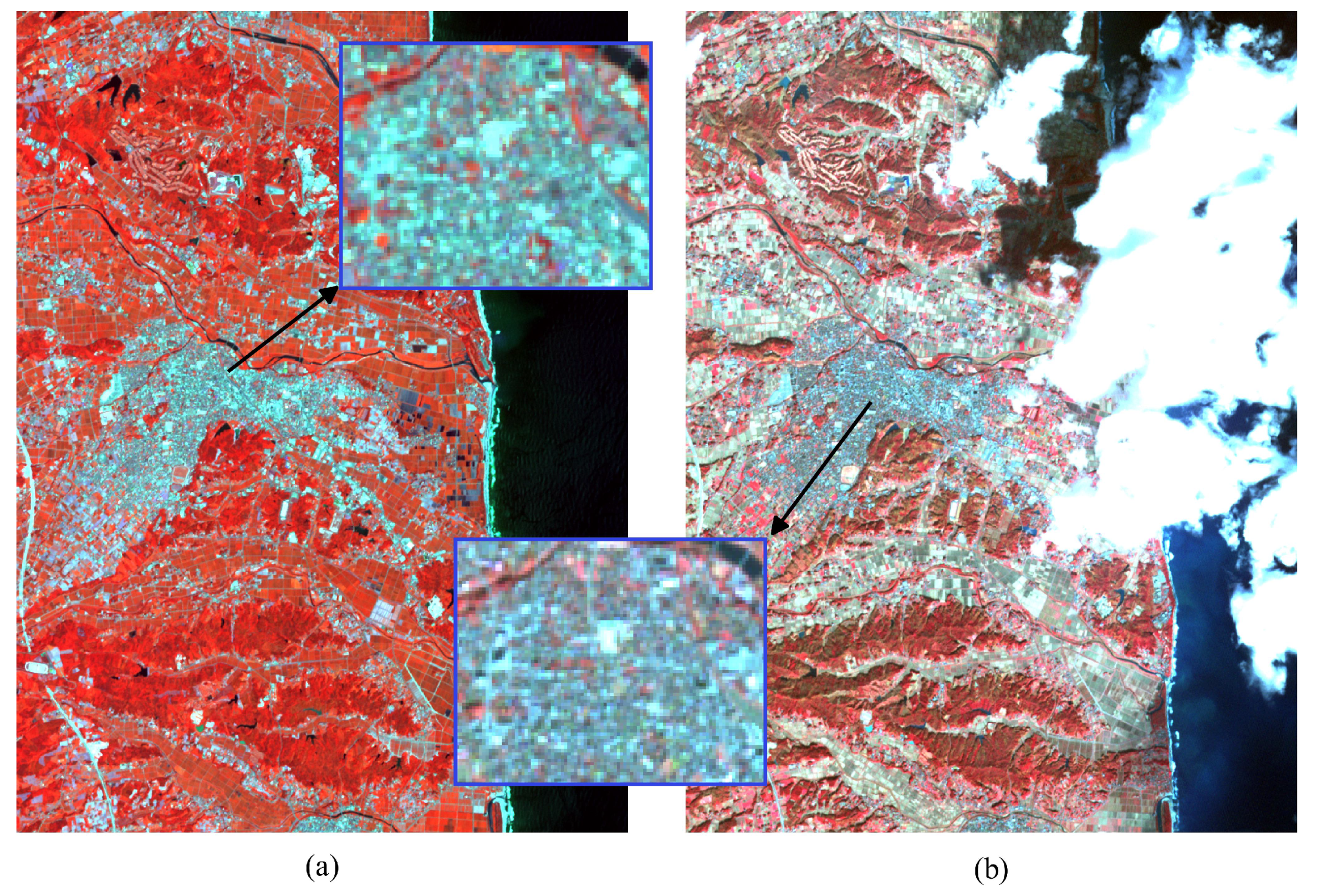
Furthermore, this analysis can be made even more difficult because of various distortions, shift and occlusion issues [3]. Some distortions are caused by the sensors themselves (calibration or the electronic components), but they may also be due to atmospheric conditions. These distortions issues may in turn cause alignments problems and difficulties to map the acquired image with GPS coordinates. In addition, finally for optical images, sometimes atmospheric conditions are simply too bad for a clean acquisition, with elements such as clouds making it impossible to take a proper picture of what is on the ground (e.g., Figure 1).
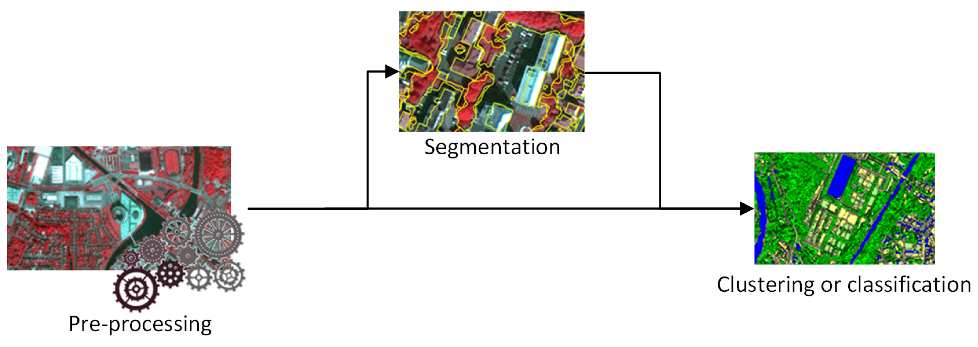
The analysis of a satellite image can usually be decomposed into 2 or 3 steps as shown in Figure 2: (1) The pre-processing step during which the image is prepared from raw sources (merging pictures, orthorectification, etc.) to solve the fore-mentioned problems; (2) an optional segmentation step that consists of grouping together adjacent pixels which are similar given a certain homogeneity criterion. These groups, called segments, should ideally be a good estimation of the objects presents in the image [4,5]; (3) Either the raw image or the segments created during step 2 can then be fed to a supervised or unsupervised machine-learning algorithm in order to recognize and classify the elements of the image.
One major issue with the analysis of satellite images is the lack of labeled data to train machine-learning algorithms, which for most of them are supervised methods that require many labeled examples to be effective. In particular, in the case of images from disasters, we have very little data that have been annotated by experts. With tsunamis, the only data we have are from the 2004 Bali tsunami and the 2011 Tohoku-Oki tsunami. Back in 2004 the resolution of satellite images was very low and the time lapse between two pictures much longer, and therefore these images cannot be reused. In addition to that, even if we had more labeled images, the variety of landscapes makes it difficult to reuse images from one disaster to another. This scarcity of labeled data is problematic in the way that many of the best machine-learning algorithms are supervised learning methods that need a lot of these labeled data to work properly. For instance, modern deep-learning architectures that are known to outperform all other machine-learning methods are supervised methods that need a very large number of the labeled data to achieve good results. It is, therefore, obvious that these architectures will not be useful when applied to satellite images of geohazards or other situations for which only few labeled data exist.
For these reasons, as many scientists working in the field of remote sensing have done [6,7,8], in this paper we will focus mostly on unsupervised learning algorithms, and more specifically unsupervised neural networks. While they still need a lot of data to be trained, they do not require these data to be labeled. These unsupervised learning methods are exploratory algorithms that try to find interesting patterns inside the data fed to them by the user. The main obvious advantage is that they avoid the cost and time to label data. However, it comes with the costs that unsupervised methods are known to give results that are usually less good than supervised ones. Indeed, the patterns and elements deemed interesting by these algorithms and found during the data exploration task are -due to the lack of supervision- not always the ones that their users expected.
In the case of this paper, the application of unsupervised AI techniques to the survey and mapping of damages caused tsunamis presents the extra difficulty that it would not be applied to one remote-sensing image, but rather 2 images (before and after the disaster) to assess the difference between them and deduce the extent of the damages. While clustering techniques as simple as the K-Means algorithm are relatively successful with remote-sensing images [2,7,8], analyzing the differences between two remote-sensing images before and after a geohazard with unsupervised techniques presents some extra difficulties [9]:
- To assess the difference, the two images pixels grids must be aligned, and the images must be perfectly orthorectified (superposition of the image and the ground). This is difficult to achieve both due to distortion issues mentioned earlier, but also because in the case of tsunamis and other geohazards, the ground or the shoreline might have changed after the disaster.
- The luminosity may be very different between the two images and thus the different bands may produce different responses leading to false positive changes.
- Depending on the time lapse between the image before and after the disaster, there may be seasonal phenomena such as changes in the vegetation or the crops that may also be mistaken for changes or damages by an unsupervised algorithm.
Within this context, one can easily see that the detection of non-trivial changes due to the tsunami itself using unsupervised learning techniques is a difficult task that requires state-of-the-art techniques in order to reach an efficiency superior to that of people sent on the ground and to map the damages within a reasonable time and with a high enough accuracy.
3. Related Works on Damage Mapping and Change Detection
Damage mapping using remote-sensing images using machine-learning algorithm is a relatively common task. It can be achieved either by directly studying post-disaster images, or by coupling change detection algorithms with images from before and after the disaster. The former only tells what is on the image while the latter tells both what changes between the two images and what categories of changes are present. The latter also reduces the amount of work since it narrows the areas to be analyzed to changed areas only. There is therefore a strong link between damage mapping for geohazards and change detection. Depending on the target application and constraints both mapping, change detection tasks, and clustering/classification tasks, may be achieved with supervised or unsupervised machine-learning algorithms. In this section, we present some related works both supervised and unsupervised, some of which were intended for geohazard damage analysis.
3.1. Supervised Methods for Change Detection and Damage Mapping
Supervised learning methods differ from unsupervised ones due to the need for annotated (manually labeled) data to train them. While they usually give better results and are more common in the literature, this need for labeled data can be a problem with automated applications for which no such data or too little data is available.
In [10], the authors propose a supervised change detection architecture based on based on U-Nets [11]. Similarly, in [12], the authors propose another and better supervised architectures based on convolutional neural networks (CNN) and that shows very good performance to separate trivial changes from non-trivial ones. This issue of detecting non-trivial changes is also a problem that we tackle in our proposed method, but in addition to these two algorithms from the state of the art, we do it using unsupervised learning thus alleviating the cost of manually labeling data. In addition, furthermore, we provide a clustering of the detected changes.
In [13], the authors proposed a weighted overlay method to detect liquefaction related damages based on the combination of data from several radar images using supervised learning methods. The supervised aspect of this work makes it quite different in spirit to what we propose in this paper due to the need for labeled data. Furthermore, as the title of the paper states this method is limited to the detection of liquefaction damages.
Closer to the application we tackle in this paper, in [14] the authors are proposing a survey of existing supervised neural networks to the same case study of the Tohoku 2011 tsunami. While this paper is close to our work both due to its application and the tools used, there are some major differences: First they propose a survey paper that use already existing neural networks (U-Nets [11] with MS Computational Network Toolkit [15]) for image segmentation, while we propose a new architecture for change detection and damage mapping. Second, they use supervised techniques and explained very well in their paper that they achieve only mild performances due to the lack of training data. Finally, they use slightly higher resolution images of a different area. However, they propose a better classification of damaged buildings with 3 classes (washed away, collapsed, intact) while we propose only the cluster associated with damaged constructions.
3.2. Unsupervised Methods for Change Detection and Damage Mapping
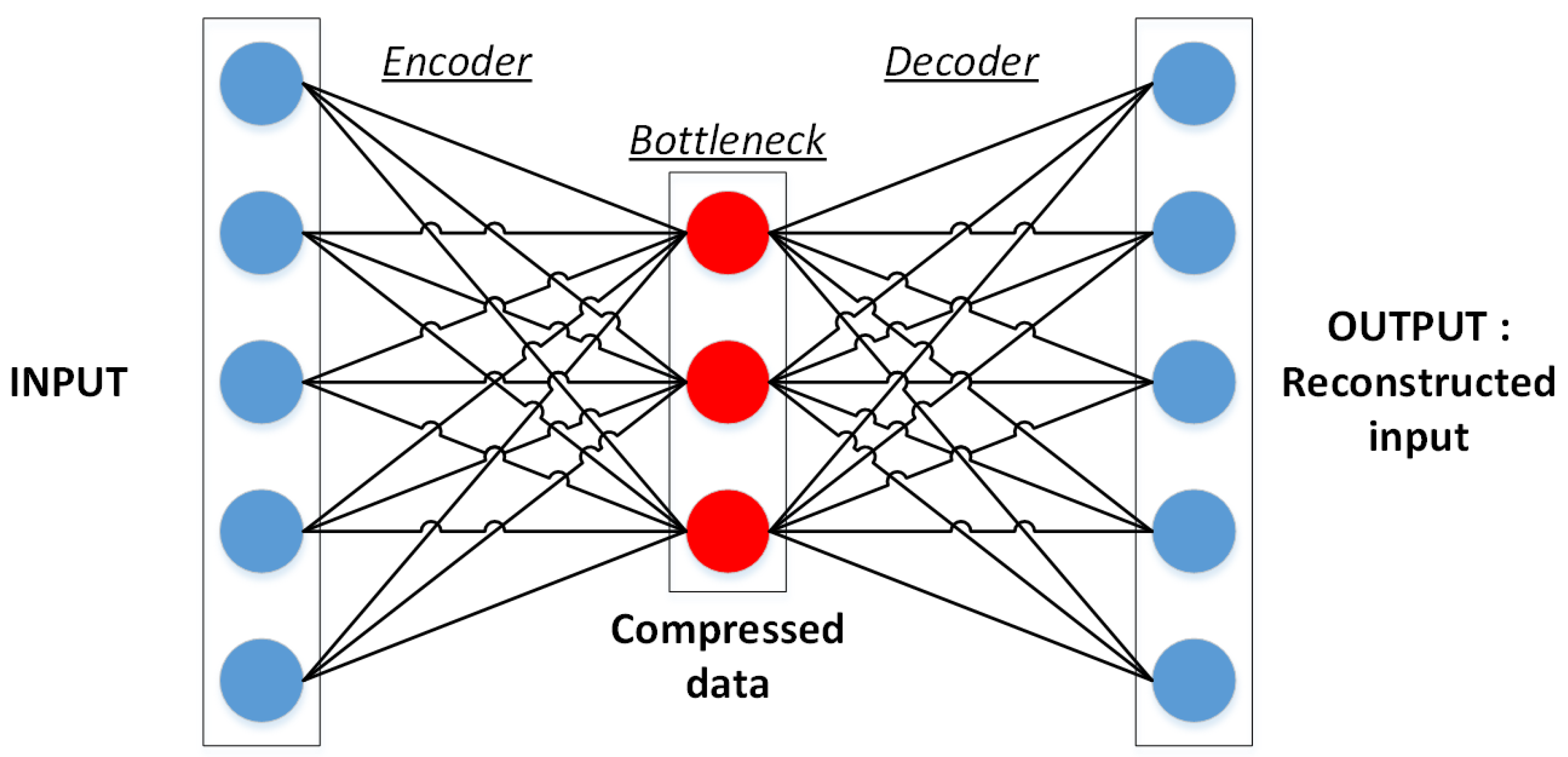
In this section, we will mention some of the main unsupervised methods from the state of the art and we will highlight their strength and weaknesses compared with our proposed approach. Most neural-based methods used for image analysis and change detection rely on autoencoders, an unsupervised type of neural network in which the input and the output are the same. In fact, the autoencoder will learn to reconstruct an output as close as possible to the original input after the information has crossed through one or several layers that extracts meaningful information from the data and/or compresses it, see Figure 3. Besides this difference that they learn to reconstruct their output instead of target labeled, autoencoders and stacked autoencoders [16] are not different from other neural networks and can be used in combination with the same convolutional layers [17] and pooling layers [18] as other neural networks. They can also be used with Fully convolutional networks (FCN) that are less costly than CNN in term of memory and are also widely used [19,20].
In [21], a regularized iteratively reweighted multivariate alteration detection (MAD) method for the detection of non-trivial changes was proposed. This method was based on linear transformations between different bands of hyperspectral satellite images and canonical correlation analysis. However, the spectral transformation between multi-temporal bands was too complex. For these reasons, deep-learning algorithms which are known to be able to model non-linear transformations, have proved their efficiency to solve this problem and have been proposed as an improvement of this architecture in [22]. In this work, the authors use an RBM-based (Restricted-Boltzmann Machines) model to learn the transformation model for a couple of VHR co-registered images. RBM is a type of stochastic artificial network that learns the distribution of the binary input data. It is considered to be simpler than convolutional and autoencoder-based neural networks, and works very well with Rectified Linear Units activation functions [23].
More recently, deep learning and neural-based methods have been proposed because they are more robust to images that are not perfectly aligned and rely on patch-wise analysis instead of pixel-based analysis. In [24], a deep architecture based on CNN and autoencoders (AE) is proposed for change detection in image time series. It relies on the encoding of two subsequent images and the subtraction of the encoded images to detect the changes. However, this approach proved to be very sensitive to changes in luminosity and seasonal changes, thus making it poorly adapted for our case study.
Alternatively, in [25], the authors propose a non-neural network-based, but still unsupervised, approach which relies on following segmented objects through time. This approach is very interesting but remains difficult to apply for cases where the changes are too big from one image to another, which is our case with radical changes caused by natural disasters such as tsunamis.
In addition to neural network-based methods, the fusion of results from several algorithms is a commonly used technique that relies on several unsupervised algorithms to increase the reliability of the analysis [26]. At the same time, automatic methods for selection of changed and unchanged pixels have also been used to obtain training samples for a multiple classifier system [27].
In [28], the authors propose another unsupervised method based on feature selection and the orientation of buildings to decide which ones are damaged or not after a disaster. Then, they compare their unsupervised method with a supervised learning method (Support Vector Machines). This study is interesting because it is limited only to buildings and it exploits geometric features with only very basic AI. Furthermore, it uses radar images and not optical ones, making it different from our study.
Our approach is described in the Section 4 and combines the advantages of the autoencoders proposed in [24] with the ability of the improved architecture from [22]. In short, we propose a change detection method which is both resistant to the noise caused by trivial changes and shift issues, gives good results by taking advantages of the strength of modern deep-learning architectures based on CNN, and provides a clustering of the detected changes.
4. Presentation of the Proposed Architecture
In this paper, we present an unsupervised approach for the estimation of damages after disasters using two images - and - from before and after the catastrophe respectively (a is for after, b is for before and images denoted with a tilde such as are for images reconstructed by an autoencoder).
The main difficulty when trying to identify changes or survey damages using unsupervised algorithms is that most methods in the literature tend to find trivial clusters caused by changes in luminosity, weather effects, changes in crops or vegetations and clusters of areas where there is no apparent changes [24,29]. Indeed, when applying clustering algorithms -deep or not- to subtractions or concatenations of two images (before and after), interesting changes such as flooding, building constructions, or destruction are a minority among all other clusters and are rarely detected. To solve this issue, in this paper we propose a two-stage architecture:
- First, we apply a joint autoencoder to detect where the non-trivial changes are. The main idea is that trivial changes from to and vice versa will be easily encoded, while the non-trivial ones will not be properly learned and will generate a high reconstruction error, thus making it possible to detect them. This idea and the architecture for this autoencoder are the main contribution of this paper.
- Second, we use the previously detected non-trivial changes as a mask and we apply a clustering algorithm only to these areas, thus avoiding potentially noisy clusters from areas without meaningful changes.
4.1. Joint Autoencoder Architecture for the Detection of Non-Trivial Changes
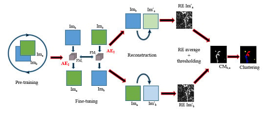
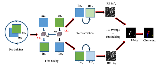
Let us begin by describing the joint autoencoder that we use to detect non-trivial changes: As stated earlier, this algorithm is based on the creation of a model that transforms into and vice versa. As it is based on unsupervised autoencoders, the model will easily learn the transformation of unchanged areas from one image to the other: seasonal changes that follow common tendency, changes in image luminosity as well as minor shift within the limit of 1–2 pixels between two images. At the same time, because the changes caused by the disaster are unique, they will be considered to be outliers by the model, and thus will have a high reconstruction error (RE). After applying a thresholding algorithm on the reconstruction values, we produce a binary change map (CM) that contains only non-trivial changes.
The algorithm steps are the following:
- The pre-processing step consists of a relative radiometrical normalization [30] if a couple of images is aligned and has enough invariant targets such as city areas that were not displaced or destructed by the disaster. It reduces the number of potential false positives and missed change alarms related to the changing in luminosity of objects.
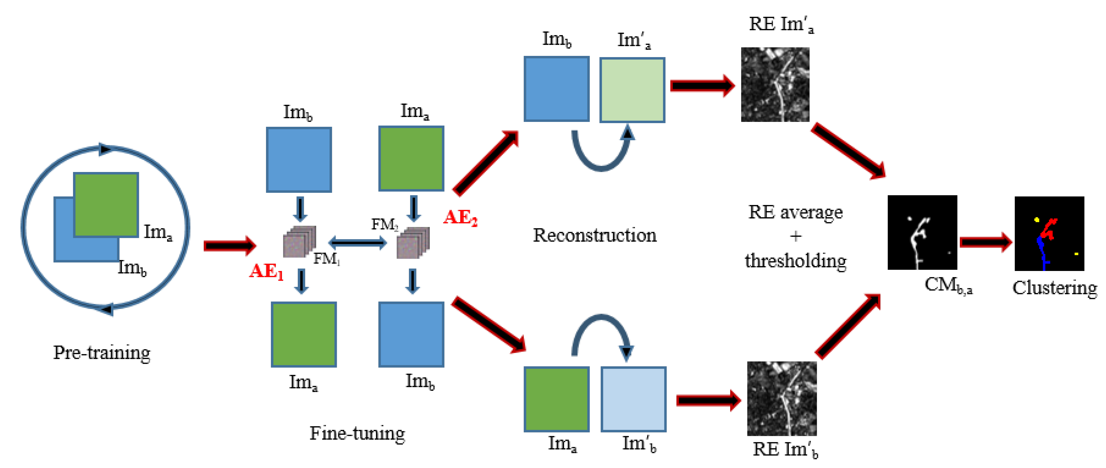
- The first step towards the detection of changes caused by disasters such as tsunamis consists of the pre-training of the transformation model (see Figure 4 and the next paragraph for the details).
- During the second step, we fine-tune the model and then calculate the RE of from and from respectively for every patch of the images. In other words, the RE of every patch is associated with the position of its central pixel on the image.
- In the third step, we identify areas of high RE using Otsu’s thresholding method [31] to create a binary change map with non-trivial change areas.
- We perform a clustering of obtained change areas to associate the detected changes to different types of damage (flooded areas, damaged buildings, destroyed elements, etc.).
- Finally, the found clusters are manually mapped to classes of interest. This process is relatively easy due to the small number of clusters and their nature which is easy to spot.
In our method, we use deep AEs to reconstruct from . During the model pre-training, the feature learning is performed patch-wise for a sample extracted from the images. In our method, we sample half of the patches from every image to prevent the model from overfitting ( patches minus the cloud mask). The patches for the border pixels are generated by mirroring the existing ones in the neighborhood. To learn the transformation model, we use fully convolutional AE. During the encoding pass of AE, the model extracts feature maps of -patch of chosen samples with convolutional layers (Figure 5), and then during the decoding pass, it reconstructs them back to the initial -patch (, , , where H is the images height, W is the images width).
The fine-tuning part consists of learning two joint reconstruction models and (see Figure 4) for every -couple of patches when trying to rebuild from and from . The patches are extracted, for every pixel of the images ( patches in total) as the local neighborhood wherein the processed pixel is the central one (i.e., the image -pixel corresponds to -patch central pixel).
The joint fully convolutional AEs model is presented in Figure 4. and have the same configuration of layers as the pre-trained model, and are initialized with the weights it learned. In the joint model, AE1 aims to reconstruct patches of from patches of and AE2 reconstructs from . The whole model is trained to minimize the difference between:
- the decoded output of AE1 and ,
- the decoded output of AE2 and ,
- the encoded outputs of AE1 and AE2.
This joint configuration where the learning is done in both temporal direction, using joint backpropagation, has empirically proven to be a lot more robust than using a regular one-way autoencoder.
To optimize the parameters of the model, we use the mean squared error (MSE) of patch reconstruction:
where x is the output patch of the model and y is the target patch.
Once the model is trained and stabilized, we perform the image reconstruction of and for every patch. For every patch, we calculate its RE using Equation (1). This gives us two images representing REs for and . Finally, we apply Otsu’s thresholding [31] that requires no parameters to the average RE of these images to produce a binary CM. However, before applying the Otsu’s thresholding we remove the 0.5% of highest values considering that they are extreme outliers more likely due to image anomalies and not changes.
4.2. Clustering of Non-Trivial Changes Areas
Once the non-trivial CM is obtained, it is used as a mask, and any clustering algorithm may be used to detect different clusters of changes on concatenated images and .
In this paper, we will compare the deep embedding clustering algorithm (DEC) [29] with more conventional clustering methods such as the K-Means algorithm [32]. These clustering algorithms are more effective when performed on concatenated versions of images and .
The main steps of the DEC algorithm are the following:
- Pre-train an AE model to extract meaningful features from the patches of concatenated images in an embedding space.
- Initialize the centers of clusters by applying classical K-Means algorithm on extracted features.
- Continue training the AE model by optimizing the AE model and the position of the centers of clusters, so the last ones are better separated. Perform label update every q iterations.
- Stop when the convergence threshold t between labels update is reached (usually ).
One of advantages of this algorithms is that if the wrong number of clusters was initialized, some clusters can be merged during the model optimization.
5. Experimental Results on the Tohoku Area Images
5.1. Presentation of the Data and Preliminary Analysis
The Tohoku tsunami was the result of a magnitude 9.1 undersea megathrust earthquake that occurred on Friday March 11th of 2011 at 2:46 p.m. local time (JST). It triggered powerful tsunami waves that may have reached heights of up to 40 m and laid waste to coastal towns of the Tohoku’s Iwate Prefecture, traveling up to 5 km inland in the Sendai area [1].
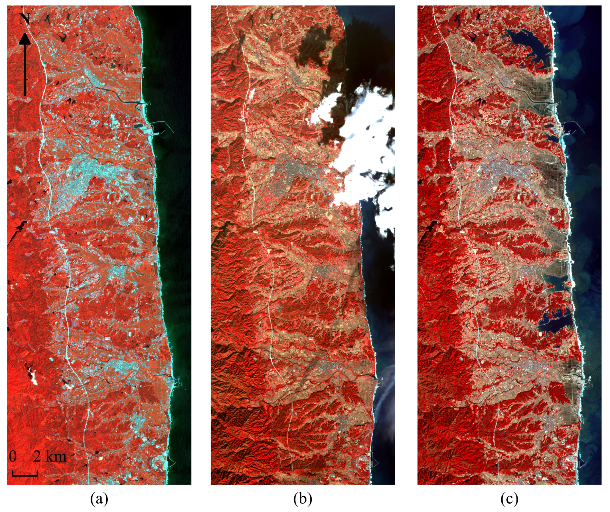
To analyze the aftermath of this disaster using the previously presented deep-learning algorithm, we use images from the ASTER program. We kept the Near-Infrared, Red and Green bands with a resolution of 15 m.
The optical images we use are from 19 March 2011, 29 November 2010 and 7 July 2010 (Figure 6), see Table 1 for their detailed characteristics. We use two images before disaster because the closest image taken on November 2010 has high percent of cloud coverage above the potentially damaged area, though it has a lower variance of seasonal changes compared with the image taken on July 2010. For this reason, we use both “before” images for change detection and we combine the two results by replacing the masked area of the November 2010 image results by the results obtained with the image taken on July 2010.
Please note that back in 2011 satellite images were taken less frequently than today, hence the gaps in time. It is also worth mentioning that open source radar images of the same area were available, but were mostly off center and with a lower resolution. For these reasons, we chose to use the optical ASTER images, rather than the radar ones, since it seems to us that they offered more possibilities. Furthermore, we insist that once again, our proposed method is generic and can work with either optical or radar images, or even a combination of both. If the same algorithm was to be applied to geohazard images today, both optical and radar images would be easily available from the day before and after the disaster, with far better resolutions.
The correction level of the images is 1C—reflectance of the top of atmosphere (TOA). It means that reflectance values are not corrected for the atmospheric effects. As the images are not perfectly aligned and most invariant targets are located close to the coast so could be destroyed, the relative image normalization is not recommended.
For the ground truth, as in [14] we use a combination of field reports and manual annotations made by our team on the post-disaster image of March 19th. Manual annotation of the data was necessary because field reports cover only a very small portion of the full image. Furthermore, flooded areas are very dependent on the date of observation and are almost fully extracted from manual annotations in our ground truth.
5.2. Algorithms Parameters
The fully convolutional AE model for change detection is presented in Table 2, where B is the number of spectral bands and p is the patch size. To detect the changes on 15 m resolution ASTER images we use patch size pixels that was chosen empirically. In the case if images were perfectly aligned, would be enough, but since we have a relatively important shift in these data, we add margins by using larger patches.
As we have two before images, we pre-train the model on the patches extracted from 3 images with the cloud mask applied (the cloud mask is extracted automatically with the K-Means algorithm using 2 clusters on the encoded images). Once the model is stabilized, we fine-tune it for 2 couples of images / and / and we calculate the RE for both couples in order to produce change maps and . We replace the masked part of by to obtain the final change map . We combined the results of two couples of images as the results produced by / are a priory more correct as the acquisition dates of the images are closer than for /. It is explained by the fact that the seasonal changes and other changes irrelevant to the disaster are less numerous. We compare the change detection results of our algorithm to RBM-based [22] change detection method because it is –to the best of our knowledge– the only unsupervised algorithm for change detection that is not sensitive to seasonal changes.
During the last step we perform the clustering of obtained change areas to associate the detected changes to different types of damage (flooded areas, damaged constructions, etc.). For this purpose, we compared 3 clustering methods:
- The K-Means algorithm applied to the subtraction of the change areas. The number of clusters was set to 3 as in final results of DEC (mentioned later).
- The K-Means algorithm applied to the encoded concatenated images of change areas (or in other words, the initialization of clusters for DEC algorithm on the pre-trained model, see step 2 of DEC algorithm in Section 4.2). The initial number of clusters was set to 4, .
- The DEC algorithm. The AE model for this algorithm is presented in Table 2. The 4 initial clusters were later reduced by algorithm to 3.
In this work, we are interested in two clusters associated with damaged constructions and flooded areas.
5.3. Experimental Results for the Detection of Non-Trivial Changes
As a first step of our experiments, we applied the joint autoencoder architecture described in the previous section to the full images to sort out the areas of non-trivial changes that may indicate modified shore line, destroyed constructions, or flooded areas. At this point, we do not attempt to sort out different types of changes, but just to have the algorithm detect areas that features changes caused by the tsunami.
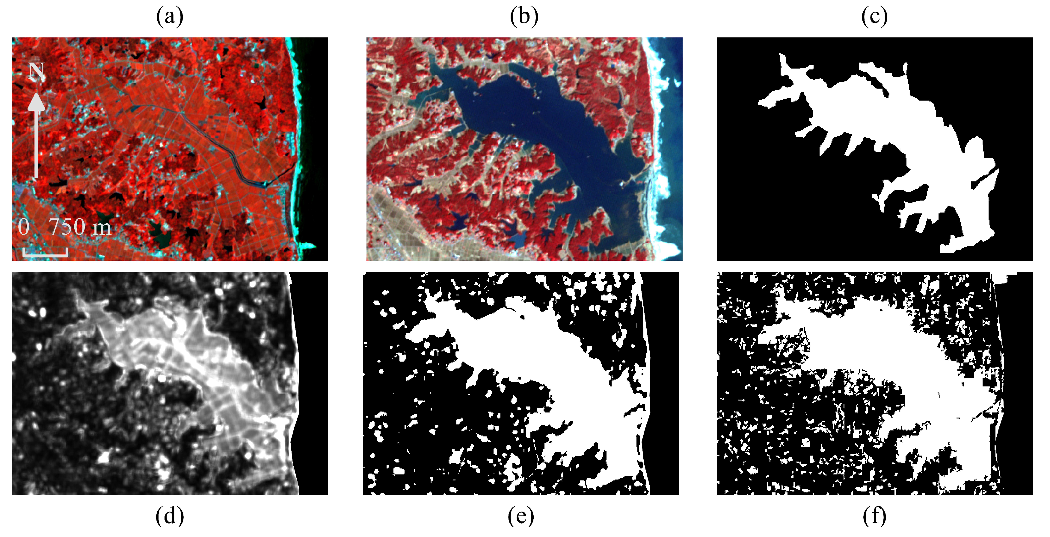
In Figure 7 and Figure 8, we highlight our results in two different zones taken in the north and south area of the image respectively: a flooded area (north area) and a destroyed city (south area). The two figures show the images from before and after the disaster, the ground truth, the result of our proposed method including the average RE image and a CM and a comparison with the results of the RBM-based approach for change detection from [22].
As one can see from the images, our proposed method is a lot less sensitive to noise than the RBM algorithm. We produce change results that are overall quite close to the ground truth. It is also worth mentioning that in Figure 8, the ground truth does not consider the shoreline modification which is clearly visible between subfigure (a) and (b) and is fully detected by our proposed algorithm, and partially detected by the RBM algorithm too.
In Table 3, we show the performance of our proposed method and the RBM method on the north and south area of the image. We compute the precision (Equation (2)), recall (Equation (3)), accuracy (Equation (4)) and Cohen’s Kappa score [33] for both methods depending on whether or not they correctly identified change area based on the ground truth. Once again, the ground truth did not include shoreline damages which may result in slightly deteriorated indexes for both algorithms.
As one can see, our proposed architecture performs significantly better than the RBM one, achieving precision, accuracy and Kappa in the northern area, and precision, recall, accuracy and Kappa in the southern area.
5.4. Experimental Results for the Clustering Step
In this subsection, we present the clustering results of the areas detected as changes in the previous step of our proposed method. As a reminder to our readers, for this step we do not propose any new clustering method and just compare existing clustering algorithms and their performance when applied after our non-trivial change detection neural network.
For an application such as damage survey after the Tohoku tsunami, we are mostly interested in detecting two types of areas: flooded areas and destroyed constructions.
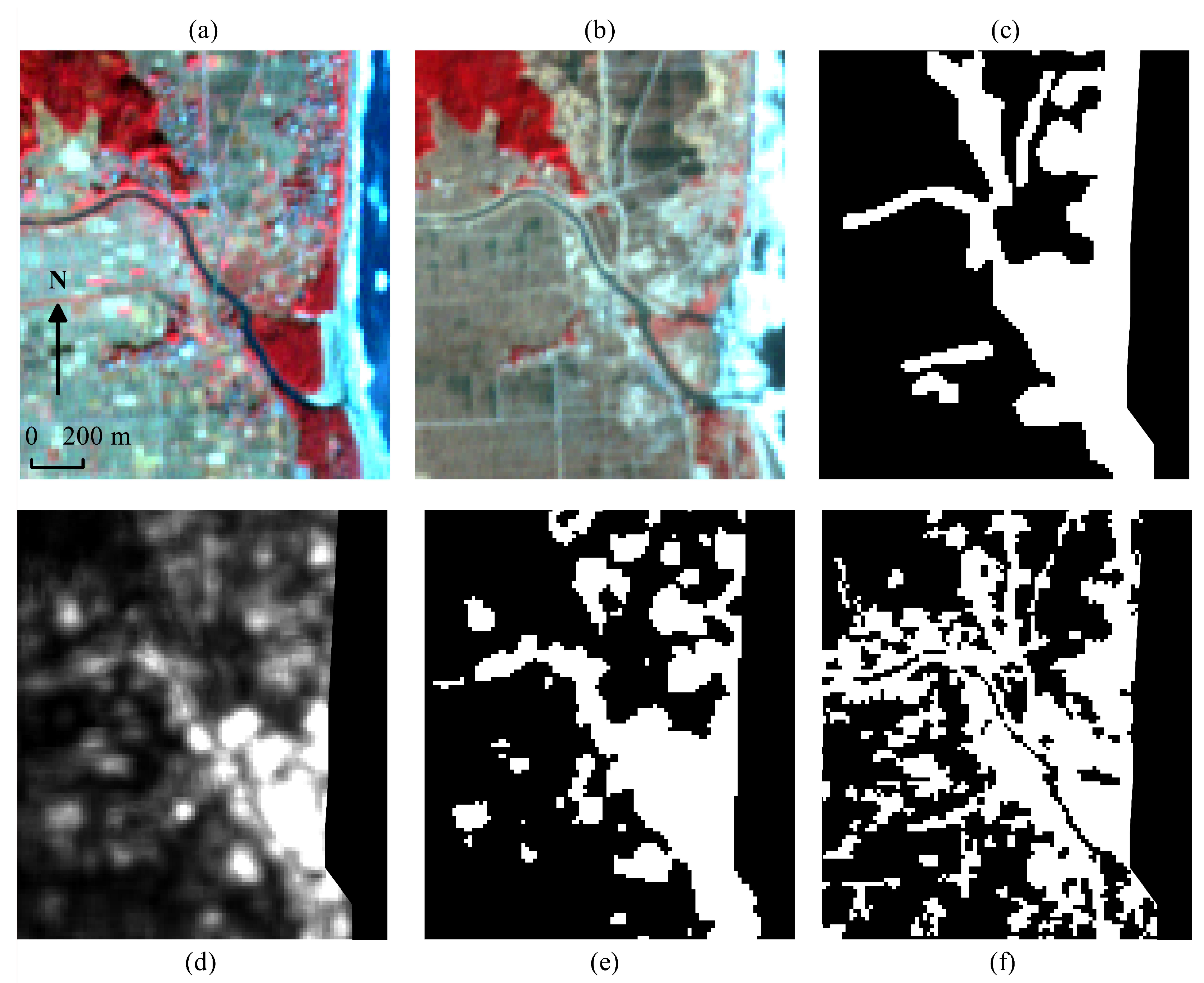
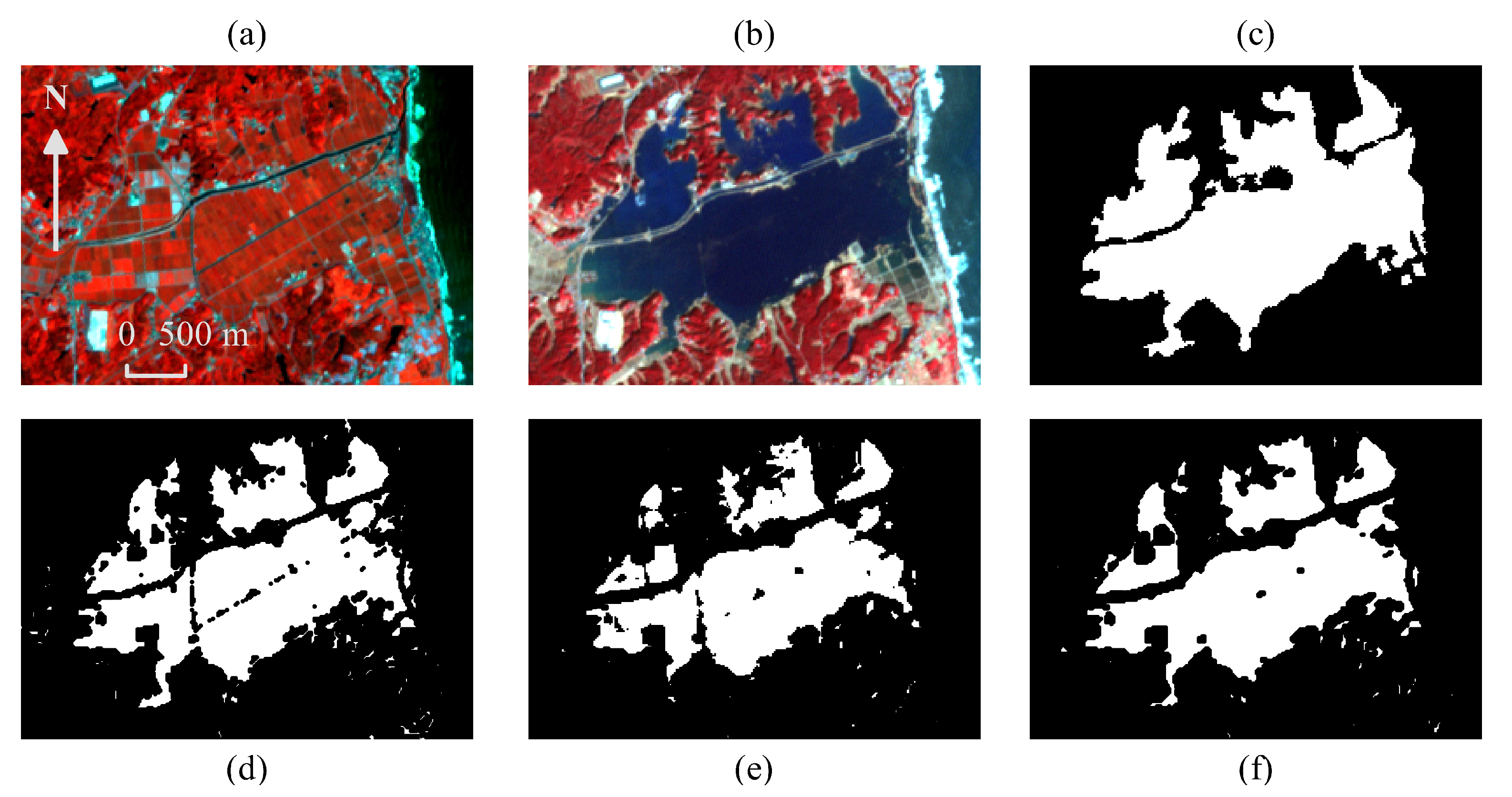
In Figure 9 we show an example of extracted clusters results for flooded areas. Images (a), (b) and (c) are the image before, after, and the ground truth, respectively. Images (d) and (e) show the results of the K-Means algorithm on subtracted and encoded concatenated images, respectively. Image (f) shows the result of the Deep Embedded Clustering algorithm. As one can see, the K-Means algorithm seems to be visually slightly better than the two other algorithms due to the homogeneity of the water cluster.
In Figure 10 we do the same for areas with destroyed buildings. Images (a), (b) and (c) are the image before, after, and the ground truth, respectively. Images (d) and (e) show the results of the K-Means algorithm on subtracted and encoded concatenated images, respectively. Image (f) shows the result of the Deep Embedded Clustering algorithm. First, we can clearly see that this damaged constructions cluster is visually a lot less accurate than the one for flooded areas. Regardless, we see that the DEC algorithm has a higher recall and Kappa score than the 2 K-Means. The low precision can be explained by the false detection of shoreline elements as damaged constructions. However, since the recall remains high at least for the DEC algorithm, we can conclude that most truly damaged constructions are properly detected but that the cluster is not pure and contains other elements.
Finally, in Table 4, we sum up the precision, recall, accuracy, and Kappa of the 3 studied clustering methods for the flooded area and damaged constructions clusters. We can see that for the water area that is relatively easy to detect, all the algorithms show similar performance. However, for destroyed buildings areas, the DEC algorithm shows the best performance on the Kappa index which characterizes the overall quality of the clustering algorithm.
We can see however that the accuracy and recall of the DEC algorithm are relatively low compared with the K-Means algorithm. This can be explained by the similar architectures (see Table 2) between our proposed method to detect non-trivial changes and the DEC algorithm. The fact that our method detects non-trivial changes based on areas that are misinterpreted may explain why a similar architecture performs only mildly on these areas. Nonetheless, the DEC algorithm still gives good results both visually and in term of Kappa index.
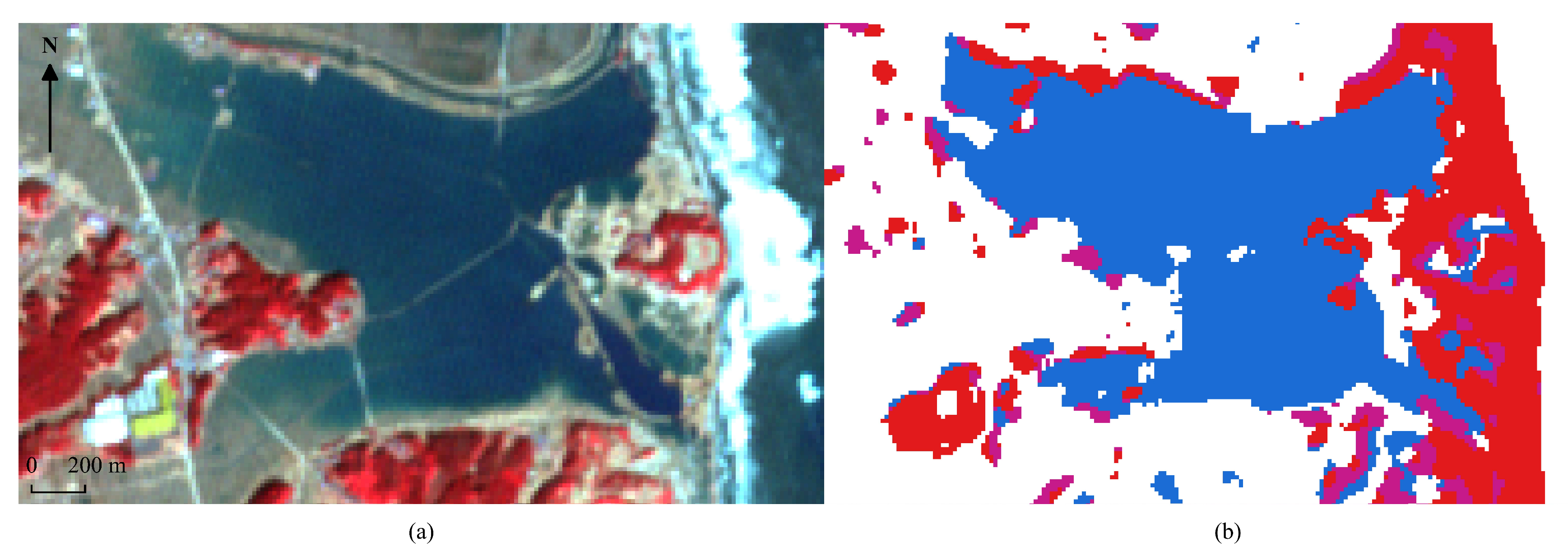
In Figure 11, we show the color clustering results with 4 clusters of the DEC algorithm on the same area than Figure 10. As one can see, we have relatively accurate results, with the main issues being once again the shoreline because of the waves, plus a bit of noise with a fourth cluster (purple color) of unknown nature being detected.
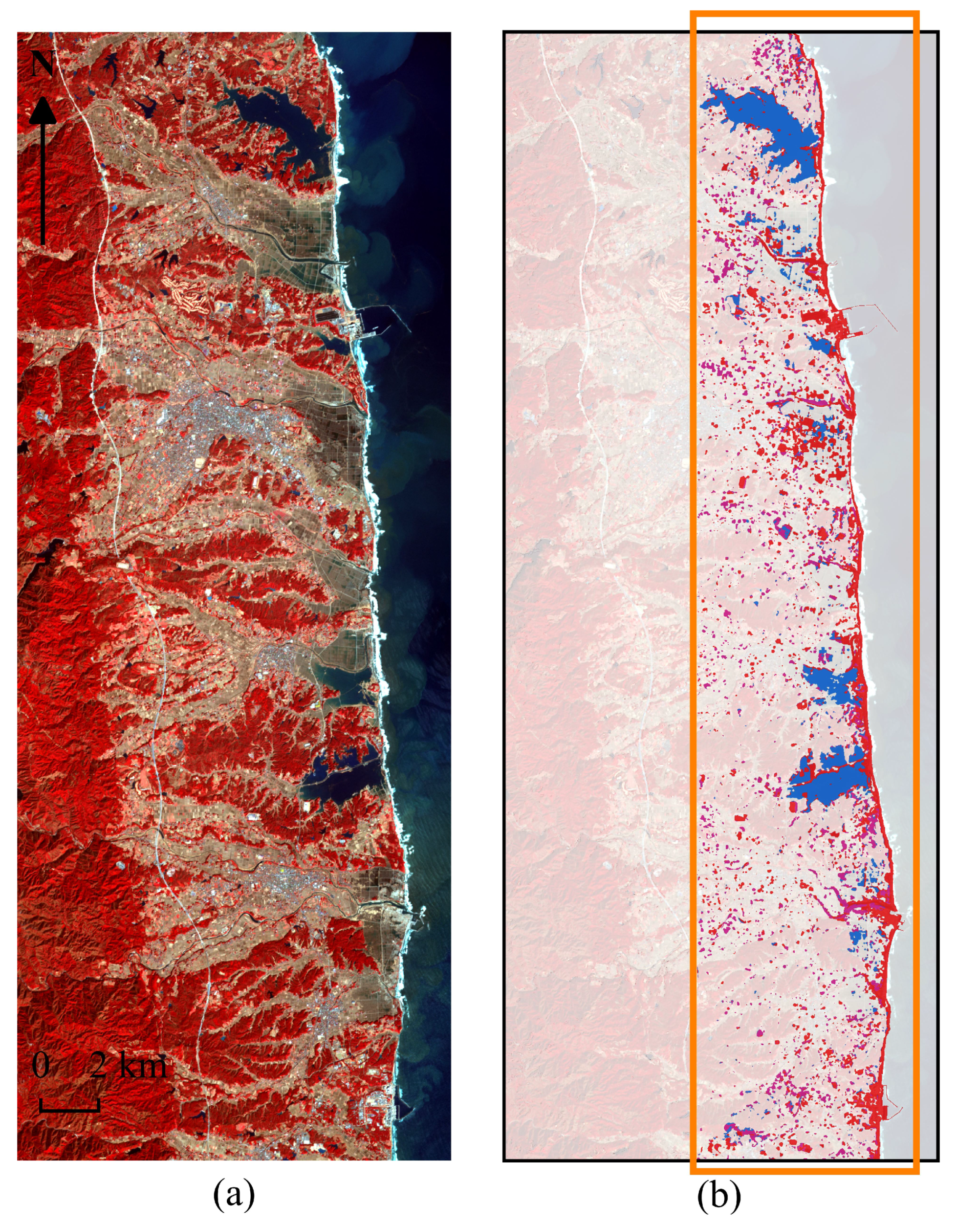
In Figure 12, we show on the left the post-disaster image and on the right the clustering of the full image after we applied the change mask and the DEC algorithm. We have the same 4 clusters: no change, flooded areas, damaged constructions, and other miscellanea changes. We can see that the issues are mostly the same as in the other Figures with a large part of the shoreline being confused with destroyed constructions which partly explains the relatively low results of precision and accuracy in Table 4 when it comes to detecting damaged constructions. It also explains the high recall since the majority of destroyed constructions are properly detected. We also see that the damages are detected mostly in valley areas and scarcer in high ground areas, which is consistent with the aftermath of the disaster.
5.5. Conclusions on the Experiments
These experiments have highlighted some of the strengths and weaknesses of our proposed methods.
First, we saw that despite being unsupervised, our algorithm is very strong to detect non-trivial changes even with relatively low-resolution images that are far apart in time, as well as cloud coverage issues and changes in luminosity. We achieve an accuracy around 85% which is comparable with supervised methods from the state of the art. This is a very strong point with an unsupervised algorithm.
Then, we also saw that the clustering phase had more mixed results, which was to be expected from an unsupervised approach. This is due to several phenomena:
- The small errors from the change detection step were propagated to the clustering step.
- It is very difficult for an unsupervised method to find clusters that perfectly match expected expert classes. Our proposed method was good enough to detect flooded areas, even when using relatively primitive machine-learning methods such as the K-Means algorithms; however damaged constructions were a lot more difficult to detect and resulted in the creation of a cluster that mixed the modified shoreline and damaged constructions. This is very obvious in Figure 11 and Figure 12 when looking at the red cluster.
- As mentioned during the presentation of the data, the ground truth is built from investigation report and manual labeling of the focus areas which means that our ground truth is far from perfect outside of these focus areas.
However, despite these difficulties, our proposed pipeline relying on joint autoencoder for change detection and the DEC algorithm for the clustering part achieve very good results for water detection, and fair results for damaged constructions detection with high recall results -thus making our point that most damaged constructions are detected but that the cluster is not pure and contain many false positive from the shoreline- and a Kappa index higher than the one achieved with the K-Means algorithm. It is worth mentioning that while they properly detected the obvious cluster of flooded areas, K-means-based approaches had even worst results at damaged constructions detection, with even the recall being of poor quality.
Finally, while the application area and the data quality are different, it is worth putting our results into perspective while comparing them with the ones from [14] where the authors proposed a state-of-the-art method for the same application of the Tohoku tsunami. The main differences are that (1) they use a supervised neural network and thus require labeled data, which we do not, and (2) they have higher quality satellite images of a different area that are not publicly available. Still, if we compare the results from their papers and ours, we can see that the various versions of U-Net they implemented achieve performances between 54.8% and 70.9% accuracy, which is not really better than the 66% of our method shown in Table 4 for damaged constructions. It proves that despite its mild performances our unsupervised algorithm is nearly as good as the state-of-the-art supervised learning method applied to better quality images. These results are in our opinion very encouraging.
As a conclusion, we can safely say that while our algorithm has room for improvement, the images from the Tohoku area in 2011 were difficult to process due to the many aforementioned issues, and we are confident that our algorithm can probably achieve better results with higher quality images.
5.6. Hardware and Software
All the experiments presented in this paper were run on a computer equipped with a NVDIA Xp Titan, an Intel Core i7 6850K, and 32 Go of DDR4 RAM. For the software part, all algorithms were implemented using Python for regular clustering methods and PyTorch for deep-learning algorithms. All visualizations were realized using QGIS.
In Table 5, we show the training and fine-tuning times for the different algorithms used in this paper.
6. Conclusions and Perspectives
In this paper, we have demonstrated how modern AI techniques can be used for automated surveys of damages after natural disasters. Using the study case of the Tohoku tsunami, we have successfully proposed and applied an unsupervised deep neural network that detect non-trivial changes in images from before and after the disaster, and then makes them very easy to process even by basic clustering algorithms to detect areas of interest such as flooded zones and damaged constructions. Our approach has shown too give fast and relatively good results while being fully unsupervised.
However, our proposed method has also shown its limits with an accuracy going no higher than 86% for change detection and around the same values for the subsequent clustering algorithms. These values, while still relatively high, are below what a good supervised algorithm could achieve, and highlight that not requiring labeled data comes at a cost.
Another weakness of our study was the absence of high-resolution radar images at the time of the Tohoku tsunami in 2011, thus forcing us to use optical images that are hindered by atmospheric distortions and occlusions. This later issue in no way changes the validity of our work in the sense that our proposed approach can be used with both optical or radar images using the same theoretical foundations. We may explore these leads in our future works, as well as more in depths clustering methods to better separate the different areas of identified non-trivial changes.
Author Contributions
J.S. is E.K. co-advisor for her PhD thesis. He came up with the subject on change detection with unsupervised techniques, as well as the application to the case study of the Tohoku tsunami. The idea behind the change detection algorithms of this paper is shared 50/50 between the two authors. Both authors designed the experimental protocol together. E.K. handled the experiments: data selection, pre-processing, application of the filters, and application of the Deep Learning and DEC algorithms. Both authors participated equally in the interpretation of the results. Both authors participated in the redaction of the paper under the direction of J.S.
Funding
This research received no external funding.
Conflicts of Interest
The authors declare no conflict of interest.
References
- Mori, N.; Takahashi, T.; Yasuda, T.; Yanagisawa, H. Survey of 2011 Tohoku earthquake tsunami inundation and run-up. Geophys. Res. Lett. 2011, 38. [Google Scholar] [CrossRef] [Green Version]
- Sublime, J.; Troya-Galvis, A.; Puissant, A. Multi-Scale Analysis of Very High Resolution Satellite Images Using Unsupervised Techniques. Remote Sens. 2017, 9, 495. [Google Scholar] [CrossRef]
- Patel, A.; Thakkar, D. Geometric Distortion and Correction Methods for Finding Key Points:A Survey. Int. J. Sci. Res. Dev. 2016, 4, 311–314. [Google Scholar]
- Pal, N.R.; Pal, S.K. A review on image segmentation techniques. Pattern Recognit. 1993, 26, 1277–1294. [Google Scholar] [CrossRef]
- Gonzalez, R.C.; Woods, R.E. Digital Image Processing, 3rd ed.; Prentice-Hall, Inc.: Upper Saddle River, NJ, USA, 2006. [Google Scholar]
- Dong, L.; He, L.; Zhang, Q. Discriminative Light Unsupervised Learning Network for Image Representation and Classification. In Proceedings of the 23rd ACM International Conference on Multimedia, Brisbane, Australia, 26–30 October 2015; ACM: New York, NY, USA, 2015; pp. 1235–1238. [Google Scholar] [CrossRef]
- Chahdi, H.; Grozavu, N.; Mougenot, I.; Berti-Equille, L.; Bennani, Y. On the Use of Ontology as a priori Knowledge into Constrained Clustering. In Proceedings of the IEEE International Conference on Data Science and Advanced Analytics (DSAA), Montreal, QC, Canada, 17–19 October 2016. [Google Scholar]
- Chahdi, H.; Grozavu, N.; Mougenot, I.; Bennani, Y.; Berti-Equille, L. Towards Ontology Reasoning for Topological Cluster Labeling. In Proceedings of the International Conference on Neural Information Processing ICONIP (3), Kyoto, Japan, 16–21 October 2016; Lecture Notes in Computer Science; Hirose, A., Ozawa, S., Doya, K., Ikeda, K., Lee, M., Liu, D., Eds.; Springer: Cham, Switzerland, 2016; Volume 9949, pp. 156–164. [Google Scholar]
- Bukenya, F.; Yuhaniz, S.; Zaiton, S.; Hashim, M.; Kalema Abdulrahman, K. A Review and Analysis of Image Misalignment Problem in Remote Sensing. Int. J. Sci. Eng. Res. 2012, 3, 1–5. [Google Scholar]
- Lei, T.; Zhang, Q.; Xue, D.; Chen, T.; Meng, H.; Nandi, A.K. End-to-end Change Detection Using a Symmetric Fully Convolutional Network for Landslide Mapping. In Proceedings of the ICASSP 2019—2019 IEEE International Conference on Acoustics, Speech and Signal Processing (ICASSP), Brighton, UK, 12–17 May 2019; pp. 3027–3031. [Google Scholar] [CrossRef]
- Ronneberger, O.; Fischer, P.; Brox, T. U-Net: Convolutional Networks for Biomedical Image Segmentation. In Proceedings of the Medical Image Computing and Computer-Assisted Intervention (MICCAI), Munich, Germany, 5–9 October 2015; Springer: Cham, Switzerland, 2015; Volume 9351, LNCS. pp. 234–241. [Google Scholar]
- Wang, Q.; Zhang, X.; Chen, G.; Dai, F.; Gong, Y.; Zhu, K. Change detection based on Faster R-CNN for high-resolution remote sensing images. Remote Sens. Lett. 2018, 9, 923–932. [Google Scholar] [CrossRef]
- Karimzadeh, S.; Matsuoka, M. A Weighted Overlay Method for Liquefaction-Related Urban Damage Detection: A Case Study of the 6 September 2018 Hokkaido Eastern Iburi Earthquake, Japan. Geosciences 2018, 8, 487. [Google Scholar] [CrossRef]
- Bai, Y.; Mas, E.; Koshimura, S. Towards Operational Satellite-Based Damage-Mapping Using U-Net Convolutional Network: A Case Study of 2011 Tohoku Earthquake-Tsunami. Remote Sens. 2018, 10, 1626. [Google Scholar] [CrossRef]
- Seide, F.; Agarwal, A. CNTK: Microsoft’s Open-Source Deep-Learning Toolkit. In Proceedings of the 22nd ACM SIGKDD International Conference on Knowledge Discovery and Data Mining (KDD’16), San Francisco, CA, USA, 13–17 August 2016; ACM: New York, NY, USA, 2016; p. 2135. [Google Scholar] [CrossRef]
- Vincent, P.; Larochelle, H.; Lajoie, I.; Bengio, Y.; Manzagol, P. Stacked Denoising Autoencoders: Learning Useful Representations in a Deep Network with a Local Denoising Criterion. J. Mach. Learn. Res. 2010, 11, 3371–3408. [Google Scholar]
- LeCun, Y.; Bengio, Y. The Handbook of Brain Theory and Neural Networks; Chapter Convolutional Networks for Images, Speech, and Time Series; MIT Press: Cambridge, MA, USA, 1998; pp. 255–258. [Google Scholar]
- Nagi, J.; Ducatelle, F.; Di Caro, G.A.; Cireşan, D.; Meier, U.; Giusti, A.; Nagi, F.; Schmidhuber, J.; Gambardella, L.M. Max-pooling convolutional neural networks for vision-based hand gesture recognition. In Proceedings of the 2011 IEEE International Conference on Signal and Image Processing Applications (ICSIPA), Kuala Lumpur, Malaysia, 16–18 November 2011; pp. 342–347. [Google Scholar] [CrossRef]
- Long, J.; Shelhamer, E.; Darrell, T. Fully convolutional networks for semantic segmentation. In Proceedings of the 2015 IEEE Conference on Computer Vision and Pattern Recognition (CVPR), Boston, MA, USA, 7–12 June 2015; pp. 3431–3440. [Google Scholar] [CrossRef]
- Kampffmeyer, M.; Salberg, A.; Jenssen, R. Semantic Segmentation of Small Objects and Modeling of Uncertainty in Urban Remote Sensing Images Using Deep Convolutional Neural Networks. In Proceedings of the 2016 IEEE Conference on Computer Vision and Pattern Recognition Workshops (CVPRW), Las Vegas, ND, USA, 26 June–1 July 2016; pp. 680–688. [Google Scholar] [CrossRef]
- Nielsen, A.A. The Regularized Iteratively Reweighted MAD Method for Change Detection in Multi- and Hyperspectral Data. IEEE Trans. Image Process. 2007, 16, 463–478. [Google Scholar] [CrossRef] [PubMed] [Green Version]
- Xu, Y.; Xiang, S.; Huo, C.; Pan, C. Change Detection Based on Auto-encoder Model for VHR Images. Proc. SPIE 2013, 8919, 891902. [Google Scholar] [CrossRef]
- Nair, V.; Hinton, G.E. Rectified Linear Units Improve Restricted Boltzmann Machines. In Proceedings of the 27th International Conference on International Conference on Machine Learning (ICML’10), Haifa, Israel, 21–24 June 2010; Omnipress: Madison, WI, USA, 2010; pp. 807–814. [Google Scholar]
- Kalinicheva, E.; Sublime, J.; Trocan, M. Neural Network Autoencoder for Change Detection in Satellite Image Time Series. In Proceedings of the 25th IEEE International Conference on Electronics, Circuits and Systems (ICECS 2018), Bordeaux, France, 9–12 December 2018; pp. 641–642. [Google Scholar] [CrossRef]
- Khiali, L.; Ndiath, M.; Alleaume, S.; Ienco, D.; Ose, K.; Teisseire, M. Detection of spatio-temporal evolutions on multi-annual satellite image time series: A clustering based approach. Int. J. Appl. Earth Obs. Geoinf. 2019, 74, 103–119. [Google Scholar] [CrossRef]
- Du, P.; Liu, S.; Gamba, P.; Tan, K.; Xia, J. Fusion of Difference Images for Change Detection Over Urban Areas. IEEE J. Sel. Top. Appl. Earth Obs. Remote Sens. 2012, 5, 1076–1086. [Google Scholar] [CrossRef]
- Tan, K.; Jin, X.; Plaza, A.; Wang, X.; Xiao, L.; Du, P. Automatic Change Detection in High-Resolution Remote Sensing Images by Using a Multiple Classifier System and Spectral–Spatial Features. IEEE J. Sel. Top. Appl. Earth Obs. Remote Sens. 2016, 9, 3439–3451. [Google Scholar] [CrossRef]
- Ji, Y.; Sumantyo, J.T.S.; Chua, M.Y.; Waqar, M.M. Earthquake/Tsunami Damage Assessment for Urban Areas Using Post-Event PolSAR Data. Remote Sens. 2018, 10, 1088. [Google Scholar] [CrossRef]
- Guo, X.; Liu, X.; Zhu, E.; Yin, J. Deep Clustering with Convolutional Autoencoders. In Neural Information Processing; Liu, D., Xie, S., Li, Y., Zhao, D., El-Alfy, E.S.M., Eds.; Springer International Publishing: Cham, Switzerland, 2017; pp. 373–382. [Google Scholar]
- El Hajj, M.; Bégué, A.; Lafrance, B.; Hagolle, O.; Dedieu, G.; Rumeau, M. Relative Radiometric Normalization and Atmospheric Correction of a SPOT 5 Time Series. Sensors 2008, 8, 2774–2791. [Google Scholar] [CrossRef] [PubMed] [Green Version]
- Otsu, N. A Threshold Selection Method from Gray-Level Histograms. IEEE Trans. Syst. Man Cybern. 1979, 9, 62–66. [Google Scholar] [CrossRef]
- MacQueen, J. Some methods for classification and analysis of multivariate observations. In Proceedings of the Fifth Berkeley Symposium on Mathematical Statistics and Probability, Oakland, CA, USA, 27 December 1965–7 January 1966; Volume 1: Statistics. University of California Press: Berkeley, CA, USA, 1967; pp. 281–297. [Google Scholar]
- Cohen, J. A Coefficient of Agreement for Nominal Scales. Educ. Psychol. Meas. 1960, 20, 37–46. [Google Scholar] [CrossRef]
Sample Availability: All images used in this paper can be found at https://earthexplorer.usgs.gov/. The source code and image results are available from the authors. |
Figure 1.
Two ASTER images taken on (a) July 2010 and (b) November 2010. Image (a) was taken in sunny conditions that caused much higher pixel values for urban area pixels (zoomed) than for image (b). For example, the value of the same pixel of this area is equal (83, 185, 126) for (a) and (37, 63, 81) for (b). Moreover, a great part of image (b) is covered by clouds and their shadow.

Figure 2.
The 3 steps of satellite image processing.

Figure 3.
Basic architecture of a single layer autoencoder made of an encoder going from the input layer to the bottleneck and the decoder from the bottleneck to the output layers.
Figure 3.
Basic architecture of a single layer autoencoder made of an encoder going from the input layer to the bottleneck and the decoder from the bottleneck to the output layers.

Figure 4.
Algorithm flowchart.

Figure 5.
Fully convolutional AE model.

Figure 6.
Images taken over the damaged area, (a) 7 July 2010, (b) 29 November 2010, (c) 19 March 2011.
Figure 6.
Images taken over the damaged area, (a) 7 July 2010, (b) 29 November 2010, (c) 19 March 2011.

Figure 7.
Change detection results. (a) image taken on 29 November 2010, (b) image taken on 19 March 2011, (c) ground truth, (d) average RE image of the proposed method, (e) proposed method CM, (f) RBM.
Figure 7.
Change detection results. (a) image taken on 29 November 2010, (b) image taken on 19 March 2011, (c) ground truth, (d) average RE image of the proposed method, (e) proposed method CM, (f) RBM.

Figure 8.
Change detection results. (a) image taken on 7 July 2010, (b) image taken on 19 March 2011, (c) ground truth, (d) average RE image of the proposed method, (e) proposed method CM, (f) RBM.
Figure 8.
Change detection results. (a) image taken on 7 July 2010, (b) image taken on 19 March 2011, (c) ground truth, (d) average RE image of the proposed method, (e) proposed method CM, (f) RBM.

Figure 9.
Clustering results, flooded area. (a) image taken on 7 July 2010, (b) image taken on 19 March 2011, (c) ground truth, (d) K-Means on subtracted image, (e) K-Means on concatenated encoded images, (f) DEC on concatenated encoded images.
Figure 9.
Clustering results, flooded area. (a) image taken on 7 July 2010, (b) image taken on 19 March 2011, (c) ground truth, (d) K-Means on subtracted image, (e) K-Means on concatenated encoded images, (f) DEC on concatenated encoded images.

Figure 10.
Clustering results, destroyed constructions. (a) image taken on 7 July 2010, (b) image taken on 19 March 2011, (c) ground truth, (d) K-Means on subtracted image, (e) K-Means on concatenated encoded images, (f) DEC on concatenated encoded images.
Figure 10.
Clustering results, destroyed constructions. (a) image taken on 7 July 2010, (b) image taken on 19 March 2011, (c) ground truth, (d) K-Means on subtracted image, (e) K-Means on concatenated encoded images, (f) DEC on concatenated encoded images.

Figure 11.
(a) Extract of the original post-disaster image (b) Clustering results with 4 clusters from the DEC algorithm. On the left is the post-disaster image, on the right the clustering applied within a 5 km distance from the shore. We have the following clusters: (1) In white, no change. (2) In blue, flooded areas. (3) In red, damaged constructions. (4) In purple, other changes.

Figure 12.
(a) Extract of the original post-disaster image (b) Clustering results with 4 clusters from the DEC algorithm. On the left is the post-disaster image, on the right the clustering with the following clusters: (1) In white, no change. (2) In blue, flooded areas. (3) In red, damaged constructions. (4) In purple, other changes.


Table 1.
Images characteristics.
| Date | Clouds | Program | Resolution | , pixels | |
|---|---|---|---|---|---|
| 24/07/2010 | <1%, far from the coast | ||||
| 29/11/2010 | ≈15%, over the coast | ASTER | 15 m | ||
| 19/03/2011 | none |
Table 2.
Models architecture.
| Convolutional AE | Convolutional AE | |
|---|---|---|
| Change Detection | DEC | |
| encoder | Convolutional(B,32)+ReLU | |
| Convolutional(B,32)+ReLU | Convolutional(32,32)+ReLU | |
| Convolutional(32,32)+ReLU | Convolutional(32,64)+ReLU | |
| Convolutional(32,64)+ReLU | Convolutional(64,64)+ReLU | |
| Convolutional(64,64)+ReLU | MaxPooling(p) | |
| Linear(64,32)+ReLU | ||
| Linear(32,4)+ | ||
| decoder | Linear(4,32)+ReLU | |
| Linear(32,64)+ReLU | ||
| Convolutional(64,64)+ReLU | UnPooling(p) | |
| Convolutional(64,32)+ReLU | Convolutional(64,64)+ReLU | |
| Convolutional(32,32)+ReLU | Convolutional(64,32)+ReLU | |
| Convolutional(32,B)+Sigmoid | Convolutional(32,32)+ReLU | |
| Convolutional(32,B)+ReLU |
Table 3.
Performance of non-trivial change detection algorithms on ASTER images. The best results in each column are in bold.
Table 3.
Performance of non-trivial change detection algorithms on ASTER images. The best results in each column are in bold.
| Methods | Classification Performance | ||||
|---|---|---|---|---|---|
| Precision | Recall | Accuracy | Kappa | ||
| North | RBM | 0.63 | 0.98 | 0.84 | 0.65 |
| Proposed | 0.66 | 0.98 | 0.86 | 0.69 | |
| South | RBM | 0.47 | 0.62 | 0.76 | 0.38 |
| Proposed | 0.60 | 0.64 | 0.82 | 0.51 | |
Table 4.
Performance of clustering algorithms on ASTER images. The best results in each column are in bold.
Table 4.
Performance of clustering algorithms on ASTER images. The best results in each column are in bold.
| Methods | Classification Performance | ||||
|---|---|---|---|---|---|
| Precision | Recall | Accuracy | Kappa | ||
| Flood areas | K-means on subtracted images | 0.90 | 0.88 | 0.91 | 0.81 |
| K-means on encoded concatenated images | 0.96 | 0.66 | 0.86 | 0.68 | |
| DEC | 0.93 | 0.82 | 0.90 | 0.80 | |
| Damaged Buildings | K-means on subtracted images | 0.57 | 0.56 | 0.86 | 0.47 |
| K-means on encoded concatenated images | 0.66 | 0.38 | 0.87 | 0.42 | |
| DEC | 0.42 | 0.82 | 0.83 | 0.52 | |
Table 5.
Training times for the different algorithms.
| Methods | Training Times | |
|---|---|---|
| PRE-Training | Fine-Tuning | |
| RBM | 8 min | 2 min |
| Our FC AE | 18 min | 16 min |
© 2019 by the authors. Licensee MDPI, Basel, Switzerland. This article is an open access article distributed under the terms and conditions of the Creative Commons Attribution (CC BY) license (http://creativecommons.org/licenses/by/4.0/).
Share and Cite
MDPI and ACS Style
Sublime, J.; Kalinicheva, E. Automatic Post-Disaster Damage Mapping Using Deep-Learning Techniques for Change Detection: Case Study of the Tohoku Tsunami. Remote Sens. 2019, 11, 1123. https://0-doi-org.brum.beds.ac.uk/10.3390/rs11091123
AMA Style
Sublime J, Kalinicheva E. Automatic Post-Disaster Damage Mapping Using Deep-Learning Techniques for Change Detection: Case Study of the Tohoku Tsunami. Remote Sensing. 2019; 11(9):1123. https://0-doi-org.brum.beds.ac.uk/10.3390/rs11091123
Chicago/Turabian StyleSublime, Jérémie, and Ekaterina Kalinicheva. 2019. "Automatic Post-Disaster Damage Mapping Using Deep-Learning Techniques for Change Detection: Case Study of the Tohoku Tsunami" Remote Sensing 11, no. 9: 1123. https://0-doi-org.brum.beds.ac.uk/10.3390/rs11091123
Note that from the first issue of 2016, this journal uses article numbers instead of page numbers. See further details here.