FORCE—Landsat + Sentinel-2 Analysis Ready Data and Beyond


Earth Observation Lab, Geography Department, Humboldt-Universität zu Berlin, Unter den Linden 6, 10099 Berlin, Germany
Remote Sens. 2019, 11(9), 1124; https://0-doi-org.brum.beds.ac.uk/10.3390/rs11091124
Submission received: 11 April 2019
/
Revised: 28 April 2019
/
Accepted: 28 April 2019
/
Published: 10 May 2019
(This article belongs to the Section Remote Sensing Image Processing)
Abstract
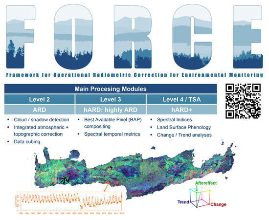
:Ever increasing data volumes of satellite constellations call for multi-sensor analysis ready data (ARD) that relieve users from the burden of all costly preprocessing steps. This paper describes the scientific software FORCE (Framework for Operational Radiometric Correction for Environmental monitoring), an ‘all-in-one’ solution for the mass-processing and analysis of Landsat and Sentinel-2 image archives. FORCE is increasingly used to support a wide range of scientific to operational applications that are in need of both large area, as well as deep and dense temporal information. FORCE is capable of generating Level 2 ARD, and higher-level products. Level 2 processing is comprised of state-of-the-art cloud masking and radiometric correction (including corrections that go beyond ARD specification, e.g., topographic or bidirectional reflectance distribution function correction). It further includes data cubing, i.e., spatial reorganization of the data into a non-overlapping grid system for enhanced efficiency and simplicity of ARD usage. However, the usage barrier of Level 2 ARD is still high due to the considerable data volume and spatial incompleteness of valid observations (e.g., clouds). Thus, the higher-level modules temporally condense multi-temporal ARD into manageable amounts of spatially seamless data. For data mining purposes, per-pixel statistics of clear sky data availability can be generated. FORCE provides functionality for compiling best-available-pixel composites and spectral temporal metrics, which both utilize all available observations within a defined temporal window using selection and statistical aggregation techniques, respectively. These products are immediately fit for common Earth observation analysis workflows, such as machine learning-based image classification, and are thus referred to as highly analysis ready data (hARD). FORCE provides data fusion functionality to improve the spatial resolution of (i) coarse continuous fields like land surface phenology and (ii) Landsat ARD using Sentinel-2 ARD as prediction targets. Quality controlled time series preparation and analysis functionality with a number of aggregation and interpolation techniques, land surface phenology retrieval, and change and trend analyses are provided. Outputs of this module can be directly ingested into a geographic information system (GIS) to fuel research questions without any further processing, i.e., hARD+. FORCE is open source software under the terms of the GNU General Public License v. >= 3, and can be downloaded from http://force.feut.de.
1. Introduction
We are currently experiencing an exciting new era of Earth observation, wherein multiple, freely available remote sensing systems provide us data at unprecedented spatial, temporal, and spectral resolutions. The Landsat mission occupies a prominent role in this development: The opening of the Landsat archive in 2008 [1] has fundamentally changed the usage of Earth observation data [2] toward mass utilization of every dataset available [3] with exponential increases in access statistics [4]. This unique long-term data record [5] is currently amended by the Sentinel-2 constellation, which provides even higher spatial, temporal, and spectral resolution [6]. Currently, the European Space Agency (ESA) and the U.S. Geological Survey (USGS) publish a daily data volume of 4 TB Sentinel-2 [7] and 1.5 TB Landsat data [8,9], thus quickly accumulating petabyte-scale archives. This regular data influx might eventually enable us to achieve sustainable development goals by closely monitoring environmental status and change at relevant scales and global extent [10,11]. However, this flood of data can easily be overwhelming, both in terms of volume and usage complexity. While the first point is merely a technical burden that can be leveled out with enough processing power and investments in storage [12], Earth observation data still need to be processed to a considerable degree before being adequate for most analyses.
Thus, there is an urgent need for data, that have been preprocessed to allow immediate analysis with a minimum of additional user effort, and which guarantee interoperability both through time and with other datasets. Such data are termed analysis ready data (ARD) (http://ceos.org/ard/), which is mostly used to describe radiometrically and geometrically consistent data that include cloud and other poor-quality observation flags for filtering data prior to analysis [13]. Whilst the development, harmonization, and provision of ARD [13,14] is a huge step forward for increasing scientific and operational uptake from broader user groups, a significant amount of processing is still necessary after having crossed the ARD barrier: (i) ARD still amount for the same, or even more, data volume than the original data; (ii) spatial and temporal variability in data availability and partial incompleteness due to clouds, acquisition orbits, and observation scenarios require specialized algorithms—or an additional round of processing—to generate spatial completeness and temporal equidistance before being ready for analysis. Therefore, it is key to go beyond ARD, and thus to provide methods and data to facilitate higher-level processing or even generate and distribute highly analysis ready data (hARD) to end users.
This paper describes the scientific, open source software FORCE (Framework for Operational Radiometric Correction for Environmental monitoring), which is being developed as an ‘all-in-one’ solution for the mass-processing and analysis of medium-resolution satellite image archives to enable both large area and time series applications. FORCE supports processing of Landsat 4/5 Thematic Mapper (TM), Landsat 7 Enhanced Thematic Mapper plus (ETM+), Landsat 8 Operational Land Imager (OLI), and Sentinel-2 A/B Multispectral Instrument (MSI) imagery. The software is capable of processing Level 1 products to Level 2–4 products, which represent different degrees of ARD. This manuscript gives an overview of the processing capabilities of FORCE version 2.1, and will end with an overview of current applications, followed by a summary on current and future improvements.
2. Product Level and Data Cube Definition
Remote sensing products are grouped in a hierarchical classification scheme [15]. The lowest available level is commonly Level 1, i.e., radiometrically calibrated and georectified data. Level 2 data most notably include some sort of atmospheric correction. Level 3 data are temporal Level 2 aggregates that are provided in a different spatial reference, commonly a grid system with a single coordinate system. Level 4 products are model output, often derived from multi-temporal or multi-sensor measurements. In this paper, Levels 1 and 2 are referred to as lower-level products and Levels 3 and above as higher-level products, respectively. Several modifications to this scheme are commonly used. As an example, Level 3 products are the first that are mapped on a regular grid, whereas the lower-level products are still in georectified swath geometry (e.g., the Landsat Worldwide Reference System 2 (WRS-2) path/row system). In contrast, the key element of ARD is to provide gridded data [13,16,17]—regardless of product level. This is for e.g., reflected in ESA’s production and distribution strategy of Sentinel-2 data as they already include gridding on Level 1 [6]—although still using local Universal Transverse Mercator (UTM) zones with a substantial amount of redundant data between overlapping and neighboring tiles.
As such, FORCE adapts gridding on Level 2, i.e., all generated products are reprojected into one coordinate system (e.g., a continental projection as in [13] or [18]), and organized in smaller tiles. The following terms are defined; see Figure 1 for a graphical representation of these concepts:
- The ‘grid’ as the regular spatial subdivision of the land surface in the target coordinate system.
- The ‘grid origin’ is the location, where the tile numbering starts with zero. Tile numbers increase toward the South and East. Although not recommended, negative tile numbers may be present if the tile origin is not North–West of the study area.
- The ‘tile’ is one entity of the grid, i.e., a grid cell with a unique tile identifier, e.g., X0003_Y0002. The tile is stationary, i.e., it always covers the same extent on the land surface.
- The ‘tile size’ is defined in target coordinate system units (most commonly in meters). Tiles are square.
- Each ‘original image’ is partitioned into several ‘chips’, i.e., any original image is intersected with the grid and then tiled into chips.
- Chips are grouped in ‘datasets’, which group data according to acquisition date and sensor. Each dataset contains several ‘products’. At minimum, a reflectance product and an accompanying quality product are generated.
- The ‘data cube’ groups all datasets within a tile in a time-ordered manner. The data cube may contain data from several sensors and different resolutions. Thus, the pixel size is allowed to vary, but the tile extent stays fixed. The data cube concept allows for non-redundant data storage and efficient data access, as well as simplified extraction of data and information.
3. Processing Capability
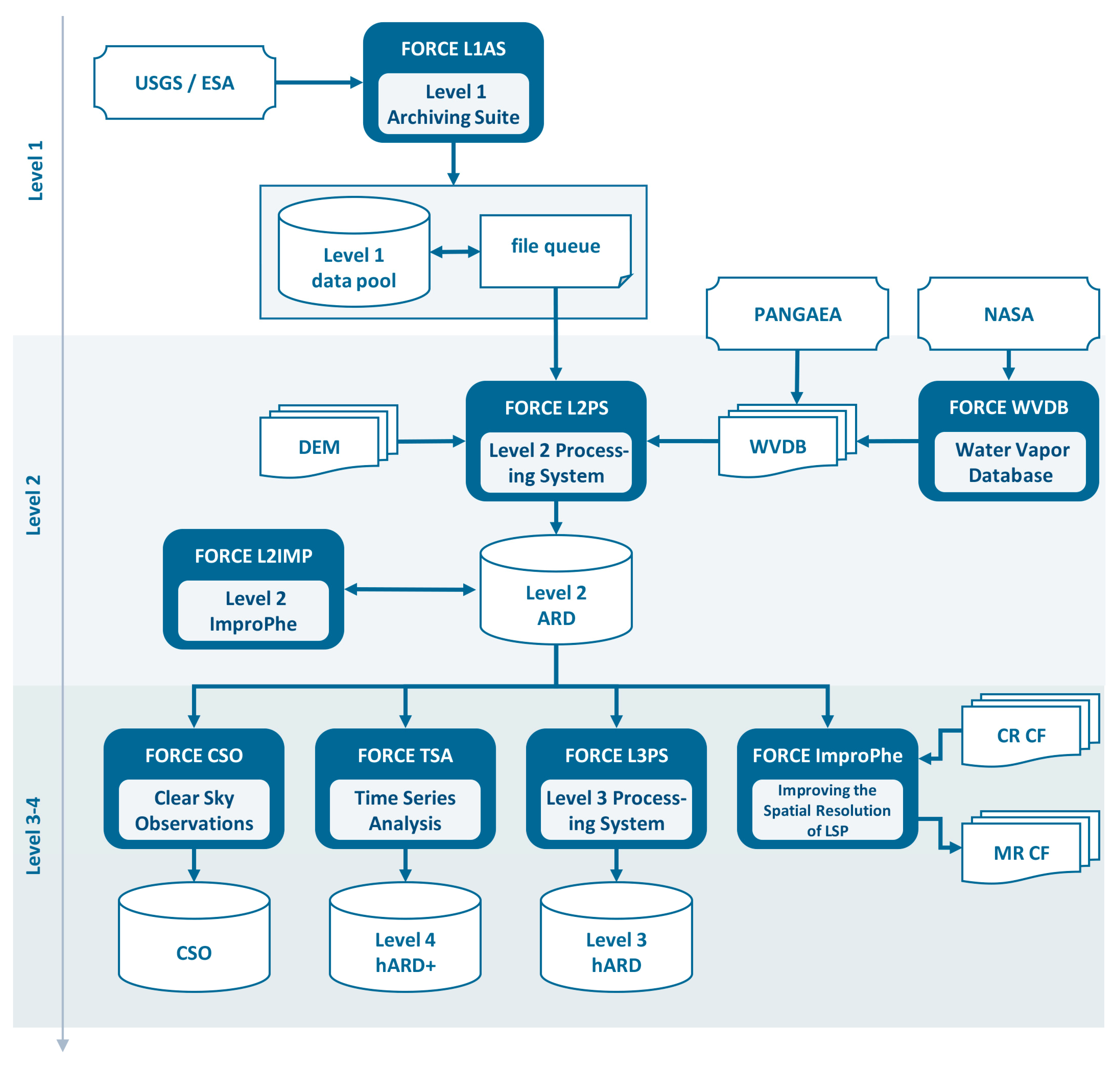
FORCE is organized in several software components. Figure 2 summarizes all available modules and their placement in the level system. A typical FORCE workflow as depicted in Figure 2 consists of following main steps: (i) Level 1 images are acquired from the space agencies, and are (ii) converted to Level 2 ARD, which are (iii) aggregated and analyzed using several higher-level modules. More detailed descriptions of the individual components will be given in the following sections, mainly ordered by level.
3.1. Level 1
The FORCE Level 1 Archiving Suite (L1AS) assists in acquiring and managing Level 1 data. L1AS has two different routines for Landsat and Sentinel-2, respectively (Figure 3). The main difference is that Landsat data need to be downloaded manually, while Sentinel-2 images are automatically retrieved by FORCE.
Once Landsat data were downloaded from USGS, L1AS ingests new images into local data holdings. L1AS keeps track of data versioning and tiers, which means outdated/lower-ranked data is replaced with newer/improved data, thus preventing data redundancy. On successful ingestion, the image is appended to a file queue, which controls Level 2 processing. The file queue is a text file that holds the full path to the image, as well as a processing-state flag. This flag is either QUEUED or DONE, which means that it is enqueued for Level 2 processing or was already processed and will be ignored next time.
The Sentinel-2 routine is similar to the one above, but ESA provides an application programming interface (API) for data query and automatic download. Based on a coordinate string list, cloud cover, and date range, a metadata report is pulled from the Copernicus API Hub. Each hit is compared with the local data holdings, and missing images are downloaded. A file queue is generated and updated accordingly.
3.2. Level 2: Analysis Ready Data
The FORCE Level 2 Processing System (FORCE L2PS) generates harmonized, standardized, and radiometrically consistent Level 2 products with per-pixel quality information, i.e., analysis ready data. L2PS pulls each enqueued Level 1 image and processes it to ARD specification. Each image (box in Figure 4) is processed independently using multiprocessing [19]. The pipeline is memory resident to minimize input/output (I/O), i.e., input data are read once, and only the final, gridded data products are written to disc.
3.2.1. Processing
The processing is based on the methodology described by Frantz et al. [18], amended by several improvements. Most prominently, support for Sentinel-2 was implemented.
Cloud masking is based on a modified version of the Fmask code [20], incorporating most updates [21] and the changes detailed by [18,22]. For Sentinel-2, the Cloud Displacement Index was developed to compensate missing thermal information employing parallax effects [23].
The spatial resolution of the 20 m Sentinel-2 bands can be improved, using the native 10 m bands as prediction targets. Three algorithms were implemented, which are listed with increasing prediction quality and processing time: (i) Spectral-only setup of the STARFM code [24], (ii) spectral-only setup of the ImproPhe code [25], and (iii) window regression [26].
Radiometric correction includes radiative-transfer-based atmospheric correction [27,28]. Aerosol optical depth is estimated over dark water and dense dark vegetation objects [29,30] using multiple scattering [18,31]. The usage of the Dark Object Database [18] to restrain aerosol optical depth estimation to permanent dark targets, was deprecated. Water vapor is estimated for each Sentinel-2 pixel; auxiliary data are used for Landsat (next section). Topographic correction is performed with an enhanced C-correction, based on the principle outlined by [32]. The C-factor is estimated for each pixel in the image and then propagated through the spectrum using radiative transfer theory. Three kernels of increasing size are used to approximate the background reflectance for environment correction [33]. Nadir BRDF-adjusted reflectance is retrieved using a global set of MODIS-derived (Moderate Resolution Imaging Spectroradiometer) BRDF kernel parameters [34,35,36].
Aerosol optical depth estimation, topographic correction effectiveness, and surface reflectance consistency was assessed for a Southern African study area [18]. The effectiveness of the topographic correction for improved forest-type classification was recently assessed in the Caucasus mountains [37]. Extended, global validation of aerosol optical depth and water vapor as well as surface reflectance were performed in the Atmospheric Correction Inter-comparison Exercise (ACIX) [38]. The parallax-based cloud detection was recently assessed in [39].
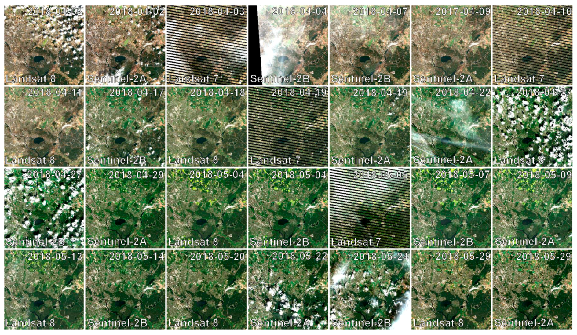
The data are reprojected to a custom projection and are then split to image chips using a custom grid with rectangular tiles, thus representing data cubes. Redundancy is prevented by aggregation of same-day/same-sensor data on output, i.e., redundant Level 1 data are not carried to Level 2. An example is shown in Figure 5.
3.2.2. Auxiliary Data
A digital elevation model (DEM) mosaic covering the complete study area is used for enhanced cloud shadow detection, scaling optical depths with altitude, and to perform the topographic correction. A precompiled water vapor database is used for atmospheric correction of Landsat data. The database holds water vapor values for the central coordinates of each WRS-2 frame. If available, day-specific values are used. If not, a monthly long-term climatology is used instead. The FORCE water vapor database component (FORCE WVDB, see Figure 2) can be used to generate and maintain such a database or a ready-to-use dataset may be freely downloaded [40]. The effect of using the water vapor climatology as a fallback option was globally assessed in [41].
3.2.3. Output Format
The gridded data are provided as compressed GeoTiff or flat binary format, accompanied by metadata. For each dataset, multiple products are stored as different files. Bottom-of-Atmosphere (BOA) reflectance (multi-band, same resolution) and quality assurance information (QAI; single band) are standard output. To homogenize and simplify usage of multi-sensor data, original band names are not carried to Level 2. Instead, specific bands can be addressed using their wavelength designation in the higher-level FORCE routines (see Table 1). The QAI product collects a number of quality-relevant status flags in bit notation (Table 2).
3.3. Higher Level: Highly Analysis Ready Data
3.3.1. General Concept
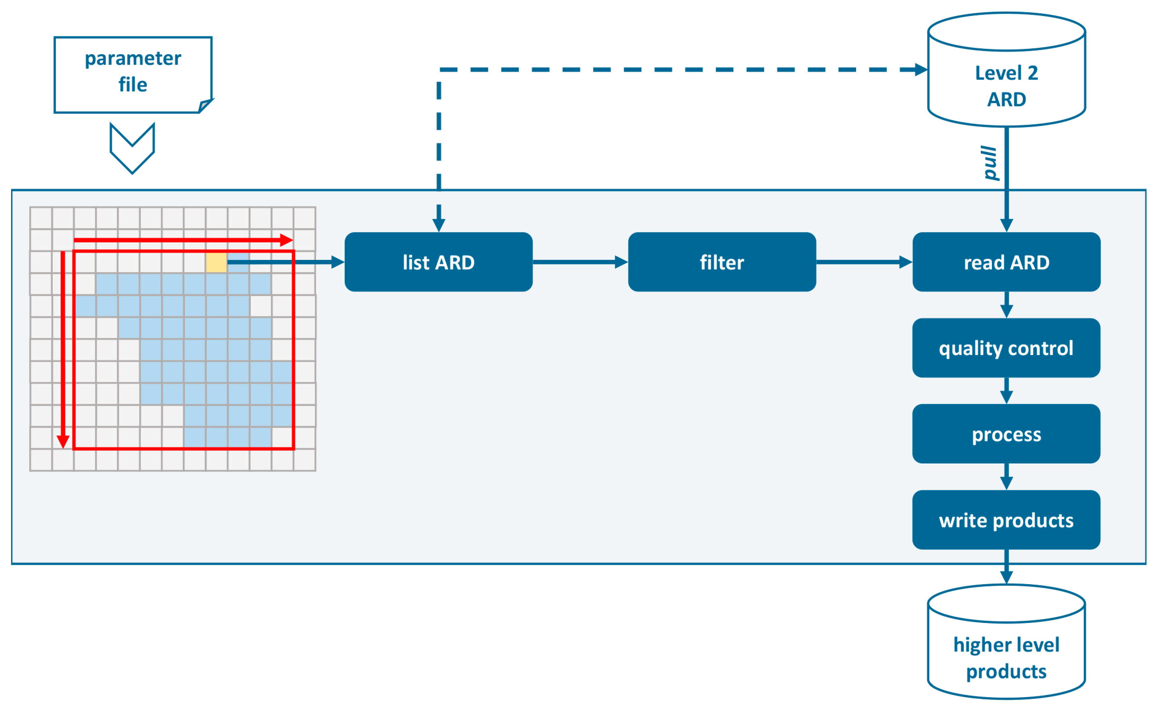
All higher-level FORCE routines follow the same general concept and act on the Level 2 ARD data cubes. The processing is tile based, i.e., the tiles are processed in sequential order (see Figure 6). Parallelization is implemented within the tile using multithreading.
FORCE reads and processes necessary information only. The square extent needs to be defined (red rectangle in Figure 6). Additionally, a tile white-list can be provided to restrict the number of tiles for non-square areas of interest (colored tiles in Figure 6). The data fusion functionalities (see Section 3.3.5) require additional data from neighboring tiles to produce seamless products; only pixels on the edge of the tiles are read (in dependence on the prediction radius). Only relevant products are pulled (in most cases, these are BOA and QAI products). The same applies to sensors, i.e., any combination of Landsat 4, 5, 7, 8, Sentinel-2A, and -2B can be chosen. A waveband mapping procedure is used to generate multi-sensor products, i.e., only matching bands are used (Table 1; for details see [42]). Spectral bands are only read when required (e.g., red and near-infrared bands for the Normalized Difference Vegetation Index (NDVI)). Temporal filters restrict the amount of data to the time period (and/or season) that is required. Output products can freely be selected, which in turn trigger the respective processing. Output is tile based; the FORCE auxiliary module (FORCE AUX) includes a tool for mosaicking generated products using the Geospatial Data Abstraction Library (GDAL) Virtual Format.
As multiple spatial resolutions are permitted within a data cube, the target resolution must be defined. Resolution adjustment can be performed using nearest-neighbor resampling (pixel decimation/replication) or reduction using approximated point spread functions (PSF). On-the-fly resolution enhancement is not implemented, but the spatial resolution of ARD can be improved beforehand (see Section 3.3.5).
Quality control is completely under the user’s control. All provided quality flags (Table 2) can be used individually.
3.3.2. Clear Sky Observations
FORCE clear sky observations (FORCE CSO) mines data availability (Figure 7), e.g., to make informed decisions about the parameterization or applicability of a specific method, or to identify areas where commissions errors reduce the amount of usable data [43]. Clear sky observations are defined in response to the quality control settings. For a given time period (in years) and interval (months), the number of clear sky observations are counted, and statistics on the temporal difference between clear sky observations are calculated; currently available statistics are the average, standard deviation, minimum, maximum, range, skewness, kurtosis, median, 25/75% quantiles, and interquartile range. The beginning and end of the intervals act as boundaries for this assessment. This processing scheme reflects the fact, that a single measure of data availability might not yield representative results. As an example (Figure 7), data availability for the first and second half of 2018 is equal in terms of the number of observations and the average time between observations. However, there are large differences in the maximum difference as data are clumped in the first half. This has important implications, e.g., for the detectability of harvesting events.
3.3.3. Level 3: Highly Analysis Ready Data
The FORCE Level 3 Processing System (FORCE L3PS) temporally condenses multi-temporal observations into a more controllable amount of spatially complete data, which lowers the usage barrier compared to Level 2 ARD. Thus, these data are referred to as highly analysis ready data (hARD). hARD products have undergone the necessary processing required for many machine-learning-based land cover/change classification purposes, which put spatial completeness before temporal exactness. Acquisition dates and quality flags of Level 2 ARD are retained as suggested by [44].
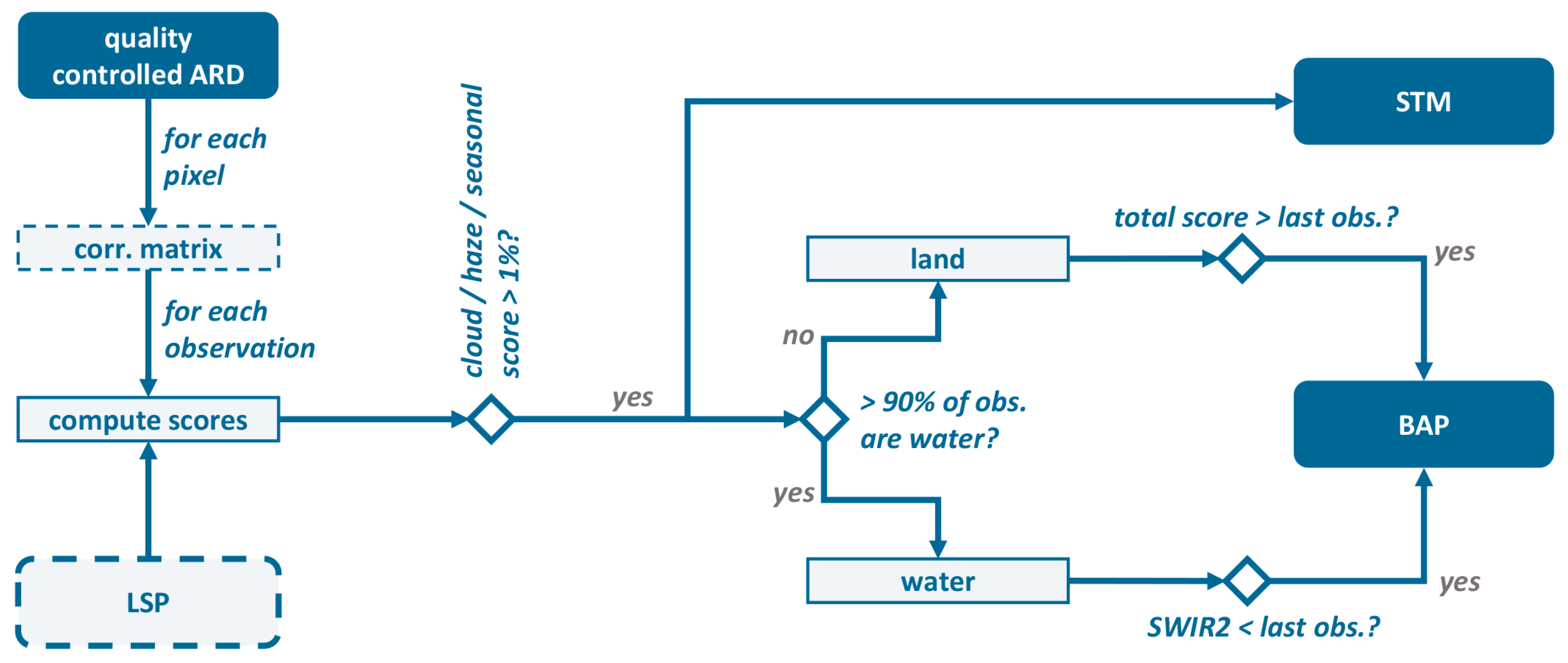
FORCE L3PS is capable of producing best-available-pixel composites [45] and spectral temporal metrics [46] (Figure 8). Both concepts utilize all available observations within a defined temporal window; best-available-pixel composites are produced by selecting the optimal observation with respect to defined criteria, whereas spectral temporal metrics are produced by a statistical description of all available spectral observations. Composites are optimal to preserve spectra for physical interpretation, but are often noisier than spectral temporal metrics. Spectral temporal metrics are produced band wise, thus physical interpretability is limited. However, they provide rich information on temporal variability and data distribution and are thus ideal predictors for machine-learning techniques that require independent features. However, their quality is closely related to data availability as a sufficient number of clear sky observations (in dependence of the statistical moment) are required to produce reliable statistics.
FORCE employs a parametric weighting scheme [45] as implemented in [47]. For each pixel, the observation with the highest total score is selected for the best-available-pixel composite. Only highest-quality pixels are considered, i.e., observations with very low cloud or haze score are discarded. Similarly, observations with very low seasonal score are discarded, which ensures that Level 3 products are representative of the season of interest (can be switched off to produce annual products). The best-available-pixel composite composites can either be parameterized using a static target date [45] or by inputting a land surface phenology dataset to dynamically adapt the target dates for each pixel [47] (example: Figure 9). Over persistent water, the compositing algorithm is switched to minimum shortwave-infrared (SWIR2 band) compositing, as the parametric weighting selection is often noisy due to the high temporal variability of water reflectance. Currently implemented spectral temporal metrics are the per-band average, standard deviation, minimum, maximum, range, skewness, kurtosis, median, 25/75% quantiles, and interquartile range of reflectance.
3.3.4. Time Series Analysis/Level 4 Highly Analysis Ready Data+
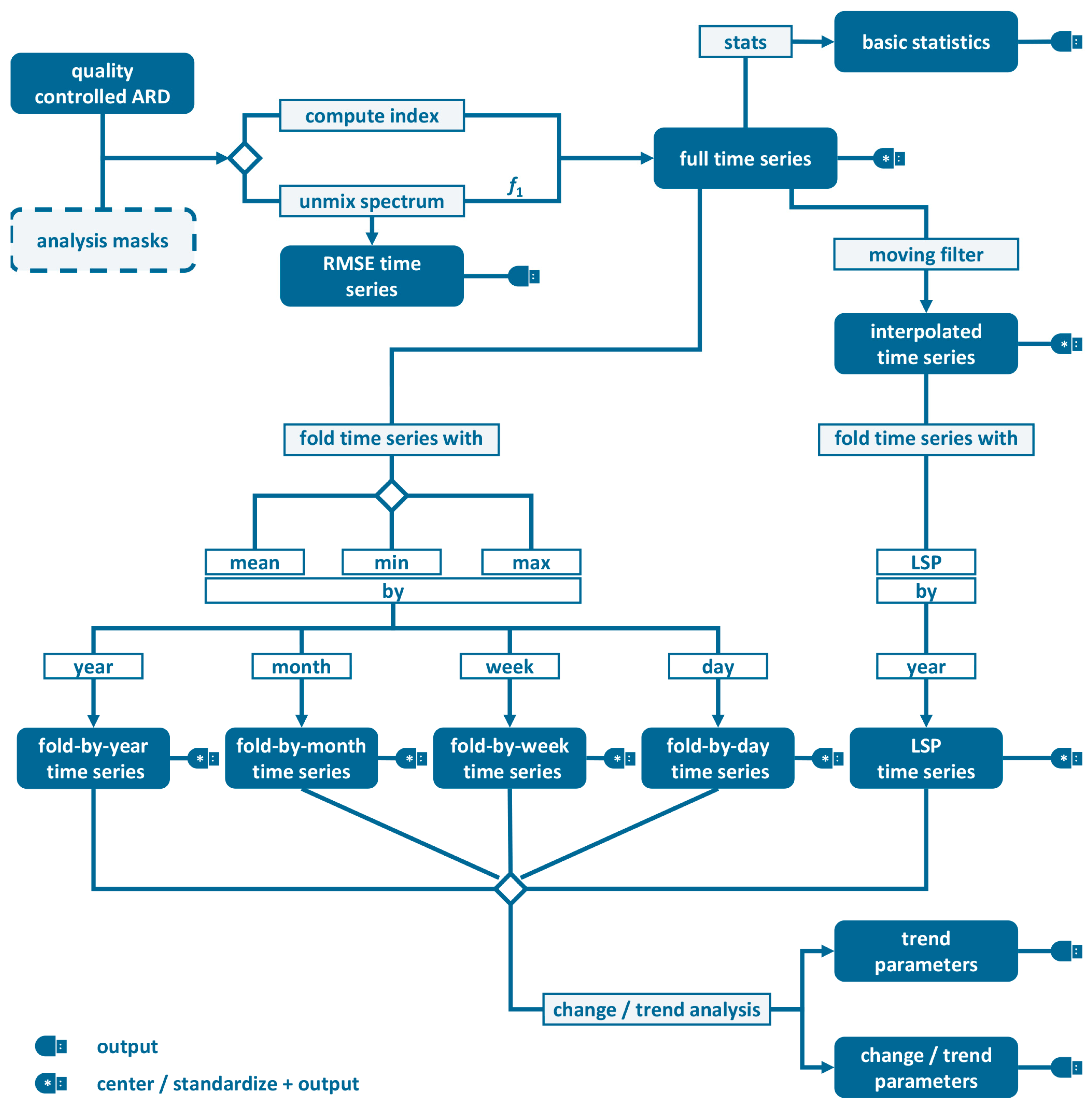
FORCE time series analysis (FORCE TSA) provides time series preparation and analysis functionality (Figure 10), i.e., extraction of quality-controlled time series with a number of aggregation and interpolation techniques, deriving land surface phenology metrics, and computing change and trend metrics. Complex processing workflows (example: Figure 11) can be executed in a single process. Many outputs of FORCE TSA are referred to as highly analysis ready data plus (hARD+), meaning that generated products can be directly ingested, analyzed, and interpreted in a geographic information system (GIS) to fuel research questions without any further processing.
Processing is based on a spectral band (Table 1), spectral index (e.g. NDVI, for a full list see [42]), or fractional cover (using linear spectral mixture analysis [48] with custom endmembers). The full time series (limited by temporal filters, see Section 3.3.1) is generated, quality-controlled, and potentially output. The time series may be centered and/or standardized each pixel’s mean and/or standard deviation before output as indication for vegetation under-/over-performance. A basic summary of the full time series can be generated, which includes per-pixel mean, standard deviation, minimum, and maximum.
The time series may be interpolated/smoothed at equidistant time steps using linear interpolation, moving average filter, and radial basis function (RBF) filter ensembles. The RBF kernel strengths are adapted by weighting with actual data availability in each kernel [49].
The full time series may be folded (aggregated) by year, month, week, or day—using mean, minimum, or maximum statistics. Folding by year is most common and generates annual time series (e.g., as employed by [50]). If folded by month, week, or day, the observations are pooled into a single virtual year, which gives up to 12, 52, or 365 values per pixel, and can, for e.g., be used to derive the long-term mean seasonality [51].
The interpolated time series may be folded by year with the land surface phenology method, i.e., annual phenometrics are extracted using the Spline Analysis of Time Series (SPLITS) API [52]. Twenty six metrics are available, which describe the timing and value of specific temporal points of interest, amplitudes, integrals, and durations.
A time series analysis can be performed on any of the folded time series. In the case of land surface phenology, the analysis is performed for each phenometric. Currently implemented analyses are linear trend analysis to derive long-term changes [53,54] and an extended change, aftereffect, trend (CAT) transform [55] with full trend parameters for the three parts of the time series (example: Figure 11).
3.3.5. Data Fusion
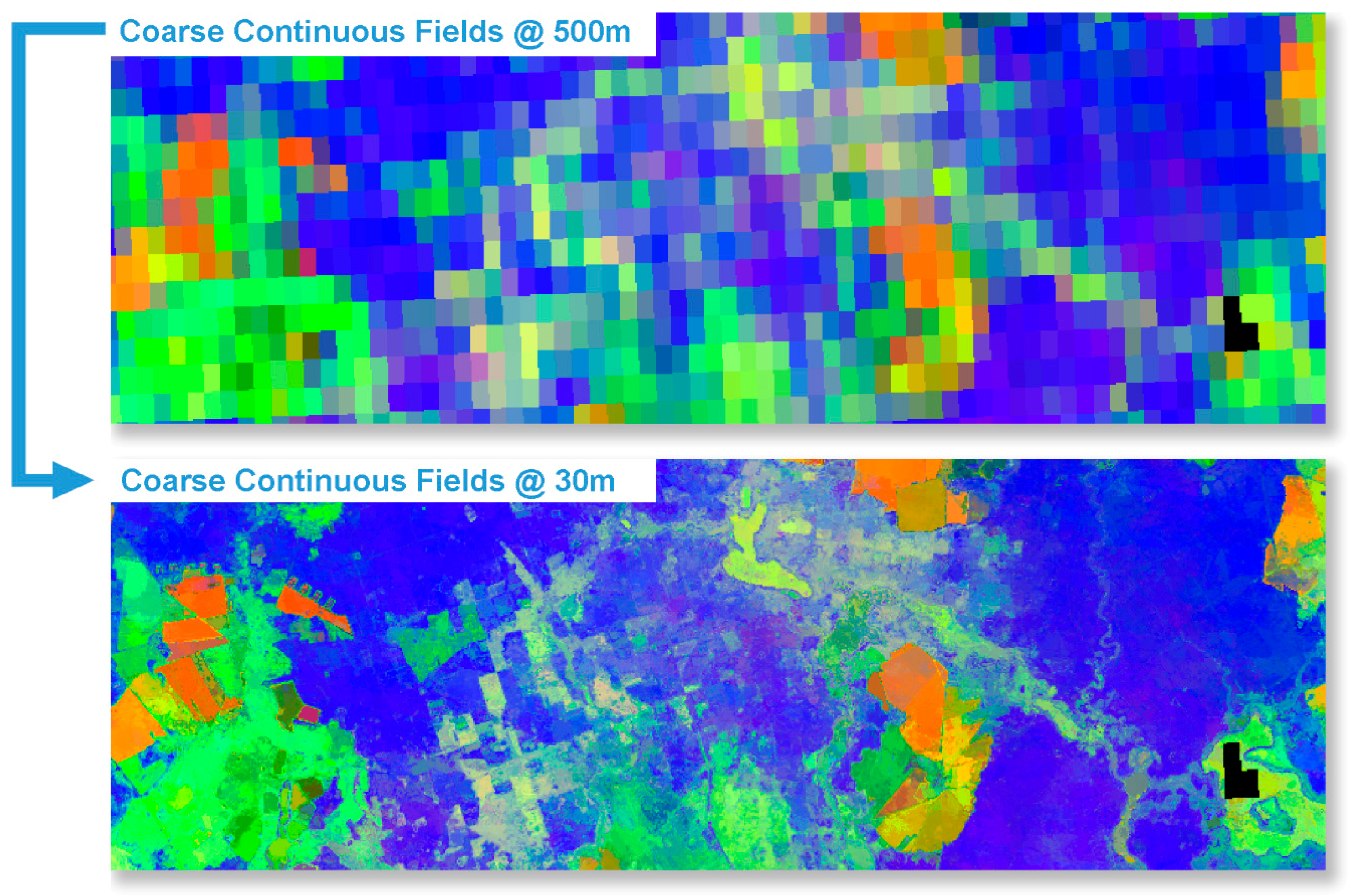
FORCE ImproPhe (Improving the spatial resolution of land surface Phenology) increases the spatial resolution of coarse continuous fields (example: Figure 12). It was originally developed to increase the spatial resolution of coarse resolution MODIS phenometrics, using Landsat ARD as multi-temporal prediction targets [25]. The fusion intensively uses the information from the local pixel neighborhood at both resolutions, wherein sparser medium resolution data are used to disentangle the land surface phenology by employing textural and spectral homogeneity metrics. ImproPhe is useful (i) in areas or times when Landsat/Sentinel-2 data are not dense enough to derive land surface phenology directly, and (ii) in areas where inter-annual climate variation prevents the strategy of pooling multiple years to increase data density. In general, ImproPhe can be applied to any coarse continuous field, provided a link to spectral–temporal land surface processes exists.
FORCE Level 2 ImproPhe (L2IMP) is capable of improving the spatial resolution of lower-resolution ARD using higher-resolution ARD, e.g., refining Landsat images with Sentinel-2 targets (example: Figure 13). Although this function produces Level 2 data (Figure 2), the general higher-level concept (3.3.1) also applies. The higher-resolution ARD are condensed to seasonal windows, and the ImproPhe code is applied to each lower-resolution ARD dataset. The refined dataset is appended to the original dataset as a separate product; thus two surface reflectance versions are available for each date. The higher-level FORCE modules can digest this data structure, and the user can choose to use the original BOA or the refined product.
4. Implementation
FORCE is open software under the terms of the GNU General Public License v. >= 3. The software and user guide can be freely downloaded from http://force.feut.de [56]. The software was developed and tested under Ubuntu Linux operating systems. The software is mostly written in C/C++, with some auxiliary functionality implemented in bash. FORCE builds on several open source tools and libraries such as GDAL [57], the GNU Scientific Library (GSL) [58], OpenMP [59], curl [60], and GNU parallel [19]. Optionally, FORCE can be linked with the SPLITS API [61] to enable deriving phenometrics.
5. Application
FORCE is increasingly used to support a wide range of scientific to operational applications. Landsat ARD and hARD, as well as Landsat-improved MODIS phenometrics were generated to serve as baseline products for environmental monitoring purposes in Southern Africa [62]. Landsat ARD and higher-level products have been extensively used in the Miombo forest ecosystem in central Angola (i) to evaluate the trade-off between food and timber resulting from forest to agriculture conversion [63], (ii) to assess spatio-temporal changes of smallholder cultivation patterns [64], and (iii) to detect forest areas that are being degraded [50]. Landsat ARD were used to support illuminating the discrepancy between deforestation and its social perception in Zambia [65]. Landsat hARD products were used to map cropping practices on a national scale in Turkey [66]. FORCE has been used in a number of conference contributions, e.g., to characterize Mediterranean land degradation due to overgrazing [67], to highlight the benefit of topographically corrected ARD for improved land cover classification [68], or as an essential building block in prototypic operational forestry applications [69].
6. Outlook
Several improvements and new features are being developed or are planned to be implemented. FORCE is open source software, and as such, external contributions are welcome. The Level 2 Processing System is currently undergoing a major overhaul to run more efficiently on weak RAM machines (e.g., common High Performance Computing (HPC) setups). Thus, memory requirements are reduced, and multithreading is implemented. Both will allow hybrid parallelization and thus enable improved flexibility with regards to different hardware architectures. As the Sentinel-2 Global Reference Image for improving geolocation accuracy [70] is still not available, and as ESA has not committed on reprocessing the available archive upon its completion, co-registration functionality is currently being implemented [71]. After having participated in the Atmospheric Correction Inter-comparison Exercise (ACIX) [38], FORCE will undergo further validation and testing in ACIX II, and the accompanying Cloud Masking Inter-comparison Exercise (CMIX) [72]. In order to support coastal aquatic applications [73], the option to output the coastal aerosol band of Landsat 8 and Sentinel-2 will be included. It is planned to implement support for Sentinel-1 data in the higher-level FORCE modules, which will need to be pre-processed similarly to the optical FORCE ARD; a fully integrated Level 2-like preprocessing tool is currently not planned by the developer, but could be contributed by interested third parties. The higher-level FORCE modules are often I/O-bound, thus measures are currently implemented to continuously pre-load data, which will reduce idle CPU times due to sequential reading–processing–writing cycles. Several software utilities are currently developed at the Earth Observation Lab, Humboldt-Universität zu Berlin: The QGIS plugins ‘EO Time Series Viewer’ [74], ‘Raster Time Series Manager’ [75], and ‘Raster Data Plotting’ [76] are being developed for visualizing mass remote sensing data at spatial, temporal, and spectral scales, and thus facilitate exploring data generated by FORCE.
Funding
The development of FORCE was supported by the Bundesministerium für Bildung und Forschung under grant number FKZ-01LG1201C (Southern African Science Service Centre for Climate Change and Adaptive Land Management Project: SASSCAL), the Bundesministerium für Verkehr und Digitale Infrastruktur under grant number FKZ-50EW1605 (Sentinel4GRIPS), and Geo.X, the Research Network for Geosciences in Berlin and Potsdam under grant number SO_087_GeoX (Near-Real Time Derivation of Land Surface Phenology using Sentinel Data: FORCE-NRT). Current development is supported by the European Research Council, grant number 741950 (Understanding the Role of Material Stock Patterns for the Transformation to a Sustainable Society: MAT_STOCKS). The APC was funded by the German Research Foundation (DFG) and the Open Access Publication Fund of Humboldt-Universität zu Berlin.
Acknowledgments
Thanks to ESA, USGS, and NASA for free and open access to Sentinel, Landsat, and MODIS data. Thanks to Patrick Hostert, Stefan Ernst and Philippe Rufin for providing feedback on the article. I want to thank the three anonymous reviewers for their constructive feedback that greatly improved the quality of this manuscript.
Conflicts of Interest
The author declares no conflict of interest.
References
- Woodcock, C.E.; Allen, R.; Anderson, M.; Belward, A.; Bindschadler, R.; Cohen, W.; Gao, F.; Goward, S.N.; Helder, D.; Helmer, E. Free Access to Landsat Imagery. Science 2008, 320, 1011a. [Google Scholar] [CrossRef]
- Wulder, M.A.; Masek, J.G.; Cohen, W.B.; Loveland, T.R.; Woodcock, C.E. Opening the Archive: How Free Data has Enabled the Science and Monitoring Promise of Landsat. Remote Sens. Environ. 2012, 122, 2–10. [Google Scholar] [CrossRef]
- Wulder, M.A.; Coops, N.C.; Roy, D.P.; White, J.C.; Hermosilla, T. Land cover 2.0. Int. J. Remote Sens. 2018, 39, 4254–4284. [Google Scholar] [CrossRef] [Green Version]
- Zhu, Z.; Wulder, M.A.; Roy, D.P.; Woodcock, C.E.; Hansen, M.C.; Radeloff, V.C.; Healey, S.P.; Schaaf, C.; Hostert, P.; Strobl, P.; et al. Benefits of the free and open Landsat data policy. Remote Sens. Environ. 2019, 224, 382–385. [Google Scholar] [CrossRef]
- Markham, B.L.; Helder, D.L. Forty-Year Calibrated Record of Earth-Reflected Radiance from Landsat: A Review. Remote Sens. Environ. 2012, 122, 30–40. [Google Scholar] [CrossRef]
- Drusch, M.; Del Bello, U.; Carlier, S.; Colin, O.; Fernandez, V.; Gascon, F.; Hoersch, B.; Isola, C.; Laberinti, P.; Martimort, P.; et al. Sentinel-2: ESA’s Optical High-Resolution Mission for GMES Operational Services. Remote Sens. Environ. 2012, 120, 25–36. [Google Scholar] [CrossRef]
- ESA. Sentinel-2 Images the Globe Every 5 Days. Available online: https://earth.esa.int/web/sentinel/missions/sentinel-2/news/-/asset_publisher/Ac0d/content/sentinel-2-images-the-globe-every-5-days (accessed on 18 March 2019).
- Roy, D.P.; Wulder, M.A.; Loveland, T.R.; Woodcock, C.E.; Allen, R.G.; Anderson, M.C.; Helder, D.; Irons, J.R.; Johnson, D.M.; Kennedy, R.; et al. Landsat-8: Science and Product Vision for Terrestrial Global Change Research. Remote Sens. Environ. 2014, 145, 154–172. [Google Scholar] [CrossRef]
- Wulder, M.A.; White, J.C.; Loveland, T.R.; Woodcock, C.E.; Belward, A.S.; Cohen, W.B.; Fosnight, E.A.; Shaw, J.; Masek, J.G.; Roy, D.P. The global Landsat archive: Status, consolidation, and direction. Remote Sens. Environ. 2016, 185, 271–283. [Google Scholar] [CrossRef]
- Pekel, J.-F.; Cottam, A.; Gorelick, N.; Belward, A.S. High-resolution mapping of global surface water and its long-term changes. Nature 2016, 540, 418. [Google Scholar] [CrossRef] [PubMed]
- Pesaresi, M.; Ehrlich, D.; Ferri, S.; Florczyk, A.; Freire, S.; Halkia, M.; Julea, A.; Kemper, T.; Soille, P.; Syrris, V. Operating procedure for the production of the Global Human Settlement Layer from Landsat data of the epochs 1975, 1990, 2000, and 2014. Publ. Off. Eur. Union 2016. [Google Scholar] [CrossRef]
- Gorelick, N.; Hancher, M.; Dixon, M.; Ilyushchenko, S.; Thau, D.; Moore, R. Google Earth Engine: Planetary-scale geospatial analysis for everyone. Remote Sens. Environ. 2017, 202, 18–27. [Google Scholar] [CrossRef]
- Dwyer, J.; Roy, D.; Sauer, B.; Jenkerson, C.; Zhang, H.; Lymburner, L. Analysis Ready Data: Enabling Analysis of the Landsat Archive. Remote Sens. 2018, 10, 1363. [Google Scholar] [CrossRef]
- Claverie, M.; Ju, J.; Masek, J.G.; Dungan, J.L.; Vermote, E.F.; Roger, J.-C.; Skakun, S.V.; Justice, C. The Harmonized Landsat and Sentinel-2 surface reflectance data set. Remote Sens. Environ. 2018, 219, 145–161. [Google Scholar] [CrossRef]
- Asrar, G.; Greenstone, R. (Eds.) MTPE EOS Reference Handbook; NASA/Goddard Space Flight Center: Greenbelt, MD, USA, 1995; p. 281.
- Hansen, M.C.; Loveland, T.R. A Review of Large Area Monitoring of Land Cover Change using Landsat Data. Remote Sens. Environ. 2012, 122, 66–74. [Google Scholar] [CrossRef]
- Frantz, D. Generation of Higher Level Earth Observation Satellite Products for Regional Environmental Monitoring. Ph.D. Thesis, Trier University, Trier, Germany, 2017. [Google Scholar]
- Frantz, D.; Röder, A.; Stellmes, M.; Hill, J. An Operational Radiometric Landsat Preprocessing Framework for Large-Area Time Series Applications. IEEE Trans. Geosci. Remote Sens. 2016, 54, 3928–3943. [Google Scholar] [CrossRef]
- Tange, O. GNU Parallel—The Command-Line Power Tool. USENIX Mag. 2011, 36, 42–47. [Google Scholar]
- Zhu, Z.; Woodcock, C.E. Object-Based Cloud and Cloud Shadow Detection in Landsat Imagery. Remote Sens. Environ. 2012, 118, 83–94. [Google Scholar] [CrossRef]
- Zhu, Z.; Wang, S.; Woodcock, C.E. Improvement and Expansion of the Fmask Algorithm: Cloud, Cloud Shadow, and Snow Detection for Landsats 4–7, 8, and Sentinel 2 Images. Remote Sens. Environ. 2015, 159, 269–277. [Google Scholar] [CrossRef]
- Frantz, D.; Röder, A.; Udelhoven, T.; Schmidt, M. Enhancing the Detectability of Clouds and Their Shadows in Multitemporal Dryland Landsat Imagery: Extending Fmask. IEEE Geosci. Remote Sens. Lett. 2015, 12, 1242–1246. [Google Scholar] [CrossRef]
- Frantz, D.; Haß, E.; Uhl, A.; Stoffels, J.; Hill, J. Improvement of the Fmask algorithm for Sentinel-2 images: Separating clouds from bright surfaces based on parallax effects. Remote Sens. Environ. 2018, 215, 471–481. [Google Scholar] [CrossRef]
- Gao, F.; Masek, J.; Schwaller, M.; Hall, F. On the Blending of the Landsat and MODIS Surface Reflectance: Predicting Daily Landsat Surface Reflectance. IEEE Trans. Geosci. Remote Sens. 2006, 44, 2207–2218. [Google Scholar] [CrossRef]
- Frantz, D.; Stellmes, M.; Röder, A.; Udelhoven, T.; Mader, S.; Hill, J. Improving the Spatial Resolution of Land Surface Phenology by Fusing Medium- and Coarse-Resolution Inputs. IEEE Trans. Geosci. Remote Sens. 2016, 54, 4153–4164. [Google Scholar] [CrossRef]
- Hill, J.; Diemer, C.; Udelhoven, T. A Local Correlation approach for the fusion of image bands with different spatial resolutions. Bull. Soc. Fr. Photogramm. Télédétect. 2003, 169, 26–34. [Google Scholar]
- Tanré, D.; Herman, M.; Deschamps, P.Y.; de Leffe, A. Atmospheric Modeling for Space Measurements of Ground Reflectances, Including Bidirectional Properties. Appl. Opt. 1979, 18, 3587–3594. [Google Scholar] [CrossRef]
- Tanré, D.; Deroo, C.; Duhaut, P.; Herman, M.; Morcrette, J.J.; Perbos, J.; Deschamps, P.Y. Description of a Computer Code to Simulate the Satellite Signal in the Solar Spectrum: The 5S Code. Int. J. Remote Sens. 1990, 11, 659–668. [Google Scholar] [CrossRef]
- Royer, A.; Charbonneau, L.; Teillet, P.M. Interannual Landsat-MSS Reflectance Variation in an Urbanized Temperate Zone. Remote Sens. Environ. 1988, 24, 423–446. [Google Scholar] [CrossRef]
- Hill, J. High Precision Land Cover Mapping and Inventory with Multi-Temporal Earth Observation Satellite Data: The Ardèche Experiment. Ph.D. Thesis, Trier University, Trier, Germany, 1993. [Google Scholar]
- Sobolev, V.V. Light Scattering in Planetary Atmospheres (Translation); Pergamon Press: Oxford, UK; New York, NY, USA, 1975; Volume 76. [Google Scholar]
- Kobayashi, S.; Sanga-Ngoie, K. The Integrated Radiometric Correction of Optical Remote Sensing Imageries. Int. J. Remote Sens. 2008, 29, 5957–5985. [Google Scholar] [CrossRef]
- Bach, H. Die Bestimmung Hydrologischer und Landwirtschaftlicher Oberflächenparameter aus Hyperspektralen Fernerkundungsdaten; Geobuch-Verlag: Munich, Germany, 1995; Volume B 21. [Google Scholar]
- Roy, D.P.; Zhang, H.K.; Ju, J.; Gomez-Dans, J.L.; Lewis, P.E.; Schaaf, C.B.; Sun, Q.; Li, J.; Huang, H.; Kovalskyy, V. A General Method to Normalize Landsat Reflectance Data to Nadir BRDF Adjusted Reflectance. Remote Sens. Environ. 2016, 176, 255–271. [Google Scholar] [CrossRef]
- Roy, D.P.; Li, J.; Zhang, H.K.; Yan, L.; Huang, H.; Li, Z. Examination of Sentinel-2A multi-spectral instrument (MSI) reflectance anisotropy and the suitability of a general method to normalize MSI reflectance to nadir BRDF adjusted reflectance. Remote Sens. Environ. 2017, 199, 25–38. [Google Scholar] [CrossRef]
- Roy, D.; Li, Z.; Zhang, H. Adjustment of Sentinel-2 Multi-Spectral Instrument (MSI) Red-Edge Band Reflectance to Nadir BRDF Adjusted Reflectance (NBAR) and Quantification of Red-Edge Band BRDF Effects. Remote Sens. 2017, 9, 1325. [Google Scholar] [CrossRef]
- Yin, H.; Tan, B.; Frantz, D.; Buchner, J.; Radeloff, V. Evaluation of topographic correction on forest mapping using Landsat imagery. (under review).
- Doxani, G.; Vermote, E.; Roger, J.-C.; Gascon, F.; Adriaensen, S.; Frantz, D.; Hagolle, O.; Hollstein, A.; Kirches, G.; Li, F.; et al. Atmospheric Correction Inter-Comparison Exercise. Remote Sens. 2018, 10, 352. [Google Scholar] [CrossRef]
- Baetens, L.; Desjardins, C.; Hagolle, O. Validation of Copernicus Sentinel-2 Cloud Masks Obtained from MAJA, Sen2Cor, and FMask Processors Using Reference Cloud Masks Generated with a Supervised Active Learning Procedure. Remote Sens. 2019, 11, 433. [Google Scholar] [CrossRef]
- Frantz, D.; Stellmes, M. Water vapor database for atmospheric correction of Landsat imagery. PANGAEA 2018. [Google Scholar] [CrossRef]
- Frantz, D.; Stellmes, M.; Hostert, P. A Global MODIS Water Vapor Database for the Operational Atmospheric Correction of Historic and Recent Landsat Imagery. Remote Sens. 2019, 11, 257. [Google Scholar] [CrossRef]
- Frantz, D. FORCE v. 2.0—Technical User Guide; ResearchGate: Berlin, Germany, 2018. [Google Scholar] [CrossRef]
- Ernst, S.; Lymburner, L.; Sixsmith, J. Implications of Pixel Quality Flags on the Observation Density of a Continental Landsat Archive. Remote Sens. 2018, 10, 1570. [Google Scholar] [CrossRef]
- Haß, E.; Frantz, D.; Mader, S.; Hill, J. Global Analysis of the Differences between the MODIS Vegetation Index Compositing Date and the Actual Acquisition Date. IEEE Geosci. Remote Sens. Lett. 2017, 14, 866–870. [Google Scholar] [CrossRef]
- Griffiths, P.; van der Linden, S.; Kuemmerle, T.; Hostert, P. A Pixel-Based Landsat Compositing Algorithm for Large Area Land Cover Mapping. IEEE J. Sel. Top. Appl. Earth Observ. Remote Sens. 2013, 6, 2088–2101. [Google Scholar] [CrossRef]
- Müller, H.; Rufin, P.; Griffiths, P.; Barros Siqueira, A.J.; Hostert, P. Mining dense Landsat time series for separating cropland and pasture in a heterogeneous Brazilian savanna landscape. Remote Sens. Environ. 2015, 156, 490–499. [Google Scholar] [CrossRef] [Green Version]
- Frantz, D.; Röder, A.; Stellmes, M.; Hill, J. Phenology-adaptive pixel-based compositing using optical earth observation imagery. Remote Sens. Environ. 2017, 190, 331–347. [Google Scholar] [CrossRef]
- Smith, M.O.; Ustin, S.L.; Adams, J.B.; Gillespie, A.R. Vegetation in deserts: I. A regional measure of abundance from multispectral images. Remote Sens. Environ. 1990, 31, 1–26. [Google Scholar] [CrossRef]
- Schwieder, M.; Leitão, P.J.; da Cunha Bustamante, M.M.; Ferreira, L.G.; Rabe, A.; Hostert, P. Mapping Brazilian savanna vegetation gradients with Landsat time series. Int. J. Appl. Earth Obs. Geoinf. 2016, 52, 361–370. [Google Scholar] [CrossRef]
- Schneibel, A.; Frantz, D.; Röder, A.; Stellmes, M.; Fischer, K.; Hill, J. Using Annual Landsat Time Series for the Detection of Dry Forest Degradation Processes in South-Central Angola. Remote Sens. 2017, 9, 905. [Google Scholar] [CrossRef]
- Melaas, E.K.; Friedl, M.A.; Zhu, Z. Detecting Interannual Variation in Deciduous Broadleaf Forest Phenology using Landsat TM/ETM+ Data. Remote Sens. Environ. 2013, 132, 176–185. [Google Scholar] [CrossRef]
- Mader, S. A Framework for the Phenological Analysis of Hypertemporal Remote Sensing Data Based on Polynomial Spline Models. Ph.D. Thesis, Trier University, Trier, Germany, 2012. [Google Scholar]
- Hostert, P.; Röder, A.; Hill, J. Coupling Spectral Unmixing and Trend Analysis for Monitoring of Long-Term Vegetation Dynamics in Mediterranean Rangelands. Remote Sens. Environ. 2003, 87, 183–197. [Google Scholar] [CrossRef]
- Sonnenschein, R.; Kuemmerle, T.; Udelhoven, T.; Stellmes, M.; Hostert, P. Differences in Landsat-Based Trend Analyses in Drylands due to the Choice of Vegetation Estimate. Remote Sens. Environ. 2011, 115, 1408–1420. [Google Scholar] [CrossRef]
- Hird, J.N.; Castilla, G.; McDermid, G.J.; Bueno, I.T. A Simple Transformation for Visualizing Non-seasonal Landscape Change from Dense Time Series of Satellite Data. IEEE J. Sel. Top. Appl. Earth Observ. Remote Sens. 2016, 9, 3372–3383. [Google Scholar] [CrossRef]
- Frantz, D. FORCE—Framework for Operational Radiometric Correction for Environmental Monitoring. v. 2.1. 2018. Available online: http://force.feut.de (accessed on 9 May 2019).
- GDAL. GDAL—Geospatial Data Abstraction Library; 2.2.2; Open Source Geospatial Foundation: Chicago, IL, USA, 2017; Available online: http://www.gdal.org (accessed on 9 May 2019).
- GSL. GSL—GNU Scientific Library; 1.2; Free Software Foundation: Boston, MA, USA, 2015; Available online: https://www.gnu.org/software/gsl/ (accessed on 9 May 2019).
- OpenMP. OpenMP—The OpenMP API Specification for Parallel Programming. 4.0. 2016. Available online: https://www.openmp.org/ (accessed on 9 May 2019).
- curl. curl—Command Line Tool and Library for Transferring Data with URLs. 7.47.0. 2016. Available online: https://curl.haxx.se/ (accessed on 9 May 2019).
- Mader, S. SPLITS—Spline Analysis of Time Series. v. 1.9. 2018. Available online: http://sebastian-mader.net/splits (accessed on 9 May 2019).
- Röder, A.; Stellmes, M.; Frantz, D.; Hill, J. Remote sensing-based environmental assessment and monitoring—generation of operational baseline and enhanced experimental products in southern Africa. In Biodiversity & Ecology 6—Climate Change and Adaptive Landmanagement in Southern Africa—Assessments, Changes, Challenges, and Solutions; Revermann, R., Krewenka, K.M., Schmiedel, U., Olwoch, J.M., Helmschrot, J., Jürgens, N., Eds.; University of Hamburg: Hamburg, Germany, 2018; pp. 344–354. [Google Scholar] [CrossRef]
- Schneibel, A.; Stellmes, M.; Röder, A.; Finckh, M.; Revermann, R.; Frantz, D.; Hill, J. Evaluating the Trade-Off between Food and Timber Resulting from the Conversion of Miombo Forests to Agricultural Land in Angola Using Multi-Temporal Landsat Data. Sci. Total Environ. 2016, 548–549, 390–401. [Google Scholar] [CrossRef]
- Schneibel, A.; Stellmes, M.; Röder, A.; Frantz, D.; Kowalski, B.; Haß, E.; Hill, J. Assessment of spatio-temporal changes of smallholder cultivation patterns in the Angolan Miombo belt using segmentation of Landsat time series. Remote Sens. Environ. 2017, 195, 118–129. [Google Scholar] [CrossRef]
- Parduhn, D.; Frantz, D. Seeing deforestation in Zambia—On the discrepancy between biophysical land-use changes and social perception. In Biodiversity & Ecology 6—Climate Change and Adaptive Landmanagement in Southern AFRICA—Assessments, Changes, Challenges, and Solutions; Revermann, R., Krewenka, K.M., Schmiedel, U., Olwoch, J.M., Helmschrot, J., Jürgens, N., Eds.; University of Hamburg: Hamburg, Germany, 2018; pp. 317–323. [Google Scholar] [CrossRef]
- Rufin, P.; Frantz, D.; Ernst, S.; Rabe, A.; Griffiths, P.; Özdoğan, M.; Hostert, P. Mapping Cropping Practices on a National Scale Using Intra-Annual Landsat Time Series Binning. Remote Sens. 2019, 11, 232. [Google Scholar] [CrossRef]
- Frantz, D.; Hostert, P.; Pflugmacher, D.; van der Linden, S.; Baumann, M.; Kümmerle, T.; Röder, A.; Griffiths, P. Land Use 2.0: The role of dense time series and phenometrics. In Proceedings of the Landsat Science Team Meeting, Boulder, CO, USA, 8–10 August 2018. [Google Scholar]
- Radeloff, V.; Yin, H.; Tan, B.; Frantz, D.; Buchner, J. Topographic Correction of Landsat imagery in the Caucasus Mountains. In Proceedings of the Landsat Science Team Meeting, Boulder, CO, USA, 8–10 August 2018. [Google Scholar]
- Hill, J.; Mader, S.; Frantz, D.; Stoffels, J.; Langshausen, J.; Dietz, J.; Averdung, C.; Göpfert, J. Sentinel4GRIPS: Copernicus als Baustein der Forstverwaltung. In Proceedings of the Nationales Forum für Fernerkundung und Copernicus, Berlin, Germany, 27–29 November 2018. [Google Scholar]
- Gascon, F.; Bouzinac, C.; Thépaut, O.; Jung, M.; Francesconi, B.; Louis, J.; Lonjou, V.; Lafrance, B.; Massera, S.; Gaudel-Vacaresse, A.; et al. Copernicus Sentinel-2A Calibration and Products Validation Status. Remote Sens. 2017, 9, 584. [Google Scholar] [CrossRef]
- Yan, L.; Roy, D.P.; Zhang, H.; Li, J.; Huang, H. An Automated Approach for Sub-Pixel Registration of Landsat-8 Operational Land Imager (OLI) and Sentinel-2 Multi Spectral Instrument (MSI) Imagery. Remote Sens. 2016, 8, 520. [Google Scholar] [CrossRef]
- ESA. CEOS-WGCV ACIX II—CMIX: Atmospheric Correction Inter-Comparison Exercise—Cloud Masking Inter-Comparison Exercise. Available online: https://earth.esa.int/web/sppa/meetings-workshops/acix (accessed on 18 March 2019).
- Poursanidis, D.; Traganos, D.; Reinartz, P.; Chrysoulakis, N. On the use of Sentinel-2 for coastal habitat mapping and satellite-derived bathymetry estimation using downscaled coastal aerosol band. Int. J. Appl. Earth Obs. Geoinf. 2019, 80, 58–70. [Google Scholar] [CrossRef]
- Jakimow, B. EO Time Series Viewer. v. 0.7.20181113T2117.develop. 2018. Available online: https://plugins.qgis.org/plugins/timeseriesviewerplugin/ (accessed on 9 May 2019).
- Rabe, A. Raster Timeseries Manager. v. 1.4. 2019. Available online: https://plugins.qgis.org/plugins/rastertimeseriesmanager/ (accessed on 9 May 2019).
- Rabe, A. Raster Data Plotting. v. 1.3. 2019. Available online: https://plugins.qgis.org/plugins/rasterdataplotting/ (accessed on 9 May 2019).
Figure 1.
Overview of gridding and data cube terminology used in FORCE (Framework for Operational Radiometric Correction for Environmental monitoring).
Figure 1.
Overview of gridding and data cube terminology used in FORCE (Framework for Operational Radiometric Correction for Environmental monitoring).

Figure 2.
Overview of FORCE, general workflow. ARD—analysis ready data; hARD—highly analysis ready data; hARD+—highly analysis ready data plus; DEM—digital elevation model; CSO—clear sky observation; LSP—land surface phenology; CF—continuous field; CR—coarse resolution; MR—medium resolution; WVDB—water vapor database; ESA—European Space Agency; USGS—U.S. Geological Survey (USGS); NASA—National Aeronautics and Space Administration.

Figure 3.
FORCE Level 1 Archiving Suite (L1AS) workflow.

Figure 4.
FORCE Level 2 Processing System (L2PS) workflow. TOA—top-of-atmosphere; BT—brightness temperature; BOA—bottom-of-atmosphere; QAI—quality assurance information.
Figure 4.
FORCE Level 2 Processing System (L2PS) workflow. TOA—top-of-atmosphere; BT—brightness temperature; BOA—bottom-of-atmosphere; QAI—quality assurance information.

Figure 5.
Data cube of Landsat 7/8 and Sentinel-2 A/B Level 2 ARD for Southeast Berlin, Germany. A two-month period of true color image chips for one 30 × 30 km tile is shown.
Figure 5.
Data cube of Landsat 7/8 and Sentinel-2 A/B Level 2 ARD for Southeast Berlin, Germany. A two-month period of true color image chips for one 30 × 30 km tile is shown.

Figure 6.
General concept of higher-level FORCE processing.

Figure 7.
Processing scheme of FORCE clear sky observations (CSO).

Figure 8.
Processing workflow of the FORCE Level 3 Processing System (L3PS). STM—spectral temporal metric; BAP—best-available pixel composite.
Figure 8.
Processing workflow of the FORCE Level 3 Processing System (L3PS). STM—spectral temporal metric; BAP—best-available pixel composite.

Figure 9.
Best-available-pixel composite (near-infrared, shortwave infrared, red in RGB) for Angola, Zambia, Zimbabwe, Botswana, and Namibia. The 250, 25, and 2.5 km subsets provide different zoom levels of the composited data. The composite is temporally centered at the end of season land surface phenology metric for 2018. The land surface phenology was derived from the Moderate Resolution Imaging Spectroradiometer (MODIS), and its spatial resolution was enhanced with the FORCE ImproPhe code (see Section 3.3.5).

Figure 10.
Processing workflow of FORCE time series analysis (TSA). All products indicated by a USB plug can be output; all products indicated by * can be centered/standardized before output.
Figure 10.
Processing workflow of FORCE time series analysis (TSA). All products indicated by a USB plug can be output; all products indicated by * can be centered/standardized before output.

Figure 11.
Land surface phenology-based trend and change analysis for Crete, Greece. The change, aftereffect, trend (CAT) transformation shows both long-term (30+ years) gradual, and abrupt changes. The CAT transform was applied to the annual value of base-level phenometric time series, which was itself derived by inferring land surface phenology metrics from dense time series of green vegetation abundance, derived from spectral mixture analysis (SMA) of Landsat ARD.

Figure 12.
Land surface phenology metrics at coarse resolution (MODIS-derived, 500 m) and with improved spatial resolution at 30 m for an image subset in Brandenburg, Germany. Depicted are (rate of maximum rise, integral of green season, and value of early minimum in RGB). Using the FORCE ImproPhe module, the spatial resolution was enhanced using multi-temporal Landsat and Sentinel-2 A/B prediction targets.

Figure 13.
Landsat ARD at original 30 m resolution (top), and Landsat ARD with improved spatial resolution at 10 m (bottom) for image subsets from North Rhine Westphalia, Germany. Using the FORCE L2IMP module, the spatial resolution was enhanced using multi-temporal Sentinel-2 A/B prediction targets.


Table 1.
Level 2 output bands and mapping to original Level 1 bands.
| Wavelength Designation | FORCE Level 2 Band LND0 [4,5,6,7,8] | FORCE Level 2 Band SEN2[AB] | USGS Level 1 Band Landsat 4/5/7 | USGS Level 1 Band Landsat 8 | ESA Level 1 Band Sentinel-2 A/B |
|---|---|---|---|---|---|
| BLUE | 1 | 1 | 1 | 2 | 2 |
| GREEN | 2 | 2 | 2 | 3 | 3 |
| RED | 3 | 3 | 3 | 4 | 4 |
| REDEDGE1 | - | 4 | - | - | 5 |
| REDEDGE2 | - | 5 | - | - | 6 |
| REDEDGE3 | - | 6 | - | - | 7 |
| BROADNIR | - | 7 | - | - | 8 |
| NIR | 4 | 8 | 4 | 5 | 8A |
| SWIR1 | 5 | 9 | 5 | 6 | 11 |
| SWIR2 | 6 | 10 | 7 | 7 | 12 |
Note: Level 1 bands, which are mainly intended for atmospheric characterization are used internally, but are not output.
Table 2.
Quality assurance information (QAI) description.
| Bit No. | Parameter Name | Bit Comb. | Integer | State |
|---|---|---|---|---|
| 0 | Valid data | 0 | 0 | valid |
| 1 | 1 | no data | ||
| 1–2 | Cloud state | 00 | 0 | clear |
| 01 | 1 | less confident cloud (i.e., buffered cloud 300 m) | ||
| 10 | 2 | confident, opaque cloud | ||
| 11 | 3 | cirrus | ||
| 3 | Cloud shadow flag | 0 | 0 | no |
| 1 | 1 | yes | ||
| 4 | Snow flag | 0 | 0 | no |
| 1 | 1 | yes | ||
| 5 | Water flag | 0 | 0 | no |
| 1 | 1 | yes | ||
| 6–7 | Aerosol state | 00 | 0 | estimated (best quality) |
| 01 | 1 | interpolated (mid quality) | ||
| 10 | 2 | high (aerosol optical depth > 0.6, use with caution) | ||
| 11 | 3 | fill (global fallback, low quality) | ||
| 8 | Subzero flag | 0 | 0 | no |
| 1 | 1 | yes (use with caution) | ||
| 9 | Saturation flag | 0 | 0 | no |
| 1 | 1 | yes (use with caution) | ||
| 10 | High sun zenith flag | 0 | 0 | no |
| 1 | 1 | yes (sun elevation < 15°, use with caution) | ||
| 11–12 | Illumination state | 00 | 0 | good (incidence angle < 55°, best quality for top. correction) |
| 01 | 1 | medium (incidence angle 55°–80°, good quality for top. correction) | ||
| 10 | 2 | poor (incidence angle > 80°, low quality for top. correction) | ||
| 11 | 3 | shadow (incidence angle > 90°, no top. correction applied) | ||
| 13 | Slope flag | 0 | 0 | no (cosine correction applied) |
| 1 | 1 | yes (enhanced C-correction applied) | ||
| 14 | Water vapor flag | 0 | 0 | measured (best quality, only Sentinel-2) |
| 1 | 1 | fill (scene average, only Sentinel-2) | ||
| 15 | Empty | 0 | 0 | TBD |
© 2019 by the author. Licensee MDPI, Basel, Switzerland. This article is an open access article distributed under the terms and conditions of the Creative Commons Attribution (CC BY) license (http://creativecommons.org/licenses/by/4.0/).
Share and Cite
MDPI and ACS Style
Frantz, D. FORCE—Landsat + Sentinel-2 Analysis Ready Data and Beyond. Remote Sens. 2019, 11, 1124. https://0-doi-org.brum.beds.ac.uk/10.3390/rs11091124
AMA Style
Frantz D. FORCE—Landsat + Sentinel-2 Analysis Ready Data and Beyond. Remote Sensing. 2019; 11(9):1124. https://0-doi-org.brum.beds.ac.uk/10.3390/rs11091124
Chicago/Turabian StyleFrantz, David. 2019. "FORCE—Landsat + Sentinel-2 Analysis Ready Data and Beyond" Remote Sensing 11, no. 9: 1124. https://0-doi-org.brum.beds.ac.uk/10.3390/rs11091124
Note that from the first issue of 2016, this journal uses article numbers instead of page numbers. See further details here.