Surfaces of Revolution (SORs) Reconstruction Using a Self-Adaptive Generatrix Line Extraction Method from Point Clouds

Abstract

This paper presents an automatic reconstruction algorithm of surfaces of revolution (SORs) with a self-adaptive method for generatrix line extraction from point clouds. The proposed method does not need to calculate the normal of point clouds, which can greatly improve the efficiency and accuracy of SORs reconstruction. Firstly, the rotation axis of a SOR is automatically extracted by a minimum relative deviation among the three axial directions for both tall-thin and short-wide SORs. Secondly, the projection profile of a SOR is extracted by the triangulated irregular network (TIN) model and random sample consensus (RANSAC) algorithm. Thirdly, the point set of a generatrix line of a SOR is determined by searching for the extremum of coordinate Z, together with overflow points processing, and further determines the type of generatrix line by the smaller RMS errors between linear fitting and quadratic curve fitting. In order to validate the efficiency and accuracy of the proposed method, two kinds of SORs, simple SORs with a straight generatrix line and complex SORs with a curved generatrix line are selected for comparison analysis in the paper. The results demonstrate that the proposed method is robust and can reconstruct SORs with a higher accuracy and efficiency based on the point clouds.

1. Introduction

Three-dimensional (3D) surface reconstruction of objects has been a popular research area in computer vision and remote sensing for a long time [1]. Many algorithms have been proposed for surface reconstruction, focusing on complex surfaces or irregular surfaces [2]. Surfaces of revolution (SORs) represent a class of regular surfaces which are generated by rotating a generatrix line around a rotation axis in Euclidean space [3,4]. The resulting surface, therefore, always has azimuthal symmetry, such as a cone (excluding the base), conical frustum (excluding the ends), cylinder (excluding the ends), prolate spheroid, pseudosphere, sphere, torus, etc. [5]. SORs reconstruction has been widely applied in the field of cultural heritage protection, reverse engineering, computer graphics, computer-aided design, computer-aided manufacturing, and computer vision [6,7]. They are very common in man-made objects and are of great relevance for a large number of applications. Especially, SORs play important roles in ancient artifacts, such as ancient vases, cups, and plates, and are important structural components of architecture [8]. Precise digital documentation of cultural heritage is essential for its protection and scientific studies carried out during the restoration and renovation process. Therefore, SORs reconstruction is often required for cultural heritage objects, so that in case of unintended human mistakes, conflicts, and disasters that destroy the objects, we have reference models to complement damaged records to restore them and to perform geometric deformation monitoring.

Generally, SORs can be reconstructed by two different types of data source; one is based on a single image or multiple images [9,10], and the other is based on point clouds [11,12,13,14]. Over the years, with the technological advances in terrestrial laser scanning (TLS), it is possible to produce multiple 3D point clouds of geometric objects’ surfaces with high density and high accuracy [15,16]. Therefore, with the advancement of real time, dynamic, and flexible laser scanning technology in recent years, point clouds obtained by TLS have become a major data source for SORs reconstruction [17].

To reconstruct a SOR is to determine its rotation axis and generatrix line from point clouds by TLS [18]. To estimate the rotation axis of a SOR, the existing approaches can be classified as the direct method, brute force method, and iterative method. The direct method uses 3D line geometry to classify surfaces and further find the rotation axis of a SOR by an eigenvalue problem or distance functions [19,20]. Although direct methods are quite fast, they cannot find accurate results if the input point clouds contain even moderate noise. The brute force method uses the fact that the intersection between a SOR and a plane perpendicular to its rotation axis is a circle. Then, the rotation axis is calculated by the least variation of fitted circle centers on each plane. However, the brute force method is time consuming [21]. The iterative method is first to create an initial SOR model by using a presumed rotation axis, and then to align this model with the point cloud, which results in a better estimation of the axis for the next iteration [22]. As the whole point cloud is used to fit the SOR model at each iteration step, the iterative method is time consuming as well.

For the determination of generatrix lines for SORs reconstruction, the most commonly used method is to estimate the surface normal at the data points by calculating the curvatures of point clouds of geometric objects and then solve certain approximation problems in the space of lines or the space of planes [13]. Benkő et al. [15] adopted the surface normal estimates associated with each point to show the significance of detecting translational and rotational symmetries. Qian and Huang [2] presented an algorithm to compute the axis and generatrix of a SOR in a partially sampled case. The generatrix was estimated to be a planar curve, which was determined by the plane with normal parallel to the estimated axis. Lee [11] presented an algorithm to approximate a set of unorganized points with a simple curve based on the normal of the point clouds, and an improved least-squares method was adopted to reduce a point cloud to a thin curve-like shape which is a near-best approximation of the point set. Andrews and Séquin [23] further expanded the application range of linear geometry to reconstruct SORs and helices. A well-studied approximate maximum-likelihood method was proposed to fit the kinematic surface, which solved the basis-dependence issue. Son et al. [24] proposed to automatically extract 3D points corresponding to as-built pipelines based on curvature computation. Normal consistency was adopted to mark different types of entities, such as the normal of the spherical surface through the center and the normal of the planes parallel to each other. All of the above methods usually rely heavily on the computation of local surface characteristics, such as the normal or curvatures. In the presence of those characteristics, they employ certain properties of SORs to estimate the 3D geometry. This methodology fails when the point cloud is of lower quality or is noisy. Moreover, the quality of the acquired normal of point clouds restricts the reconstructed SORs [22]. The most commonly used method to obtain the surface normal from point clouds is total linear least squares, which is relatively cheap to compute and easy to implement. However, it becomes more computationally expensive with the increase of measurements per second generated by TLS sensors [25].

With the purpose of reconstructing the initial 3D model of SORs for ancient artifacts and important structural components of ancient architectures from point cloud by TLS, this paper explores an automatic reconstruction algorithm of SORs with a self-adaptive method for generatrix line extraction from point clouds. The proposed method does not need to calculate the normal of point clouds, which can greatly improve the efficiency and accuracy of SORs reconstruction. The self-adaptive method for generatrix line extraction includes the following three key steps: (1) extract the rotation axis of a SOR by a minimum relative deviation among the three axial directions for both tall-thin and short-wide SORs automatically; (2) extract the projection profile of a SOR by triangulated irregular network (TIN) construction and random sample consensus (RANSAC) algorithm; and (3) determine the generatrix line of a SOR by searching for the extremum of coordinate Z, together with an overflow points processing, and further determine the type of generatrix line by the smaller RMS errors between linear fitting and quadratic curve fitting.

2. Methods

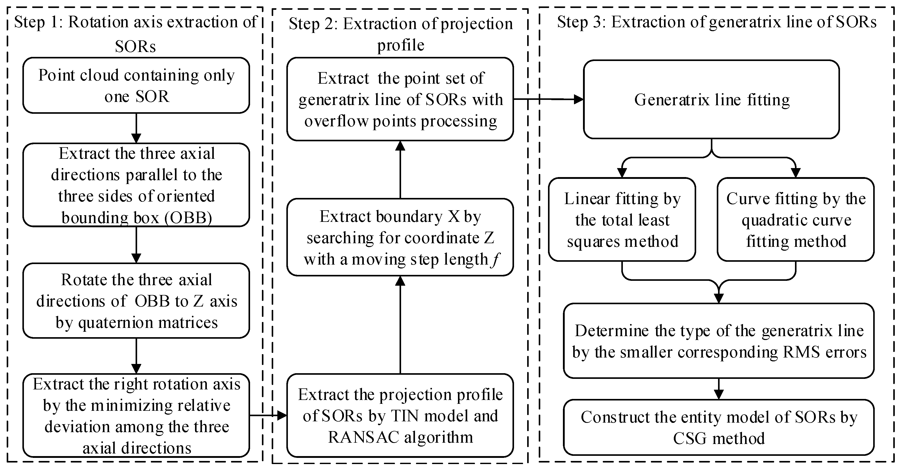
Aiming to improve the efficiency and accuracy of SORs reconstruction, an automatic reconstruction algorithm is presented for point clouds containing only one SOR without outliers, which are points far from the true surface. The outliers of the point cloud are removed by using 1.5 times resolution of the used TLS, which is searched by using the KD tree neighborhood search algorithm. If the number of obtained neighborhood points is less than one, it is an abnormal value of the point cloud and will be eliminated. Figure 1 shows the overall flowchart of the presented algorithm, which involves the following three key steps, rotation axis extraction of SORs, extraction of projection profile, and extraction of generatrix line of SORs.

2.1. Rotation Axis Extraction of SORs

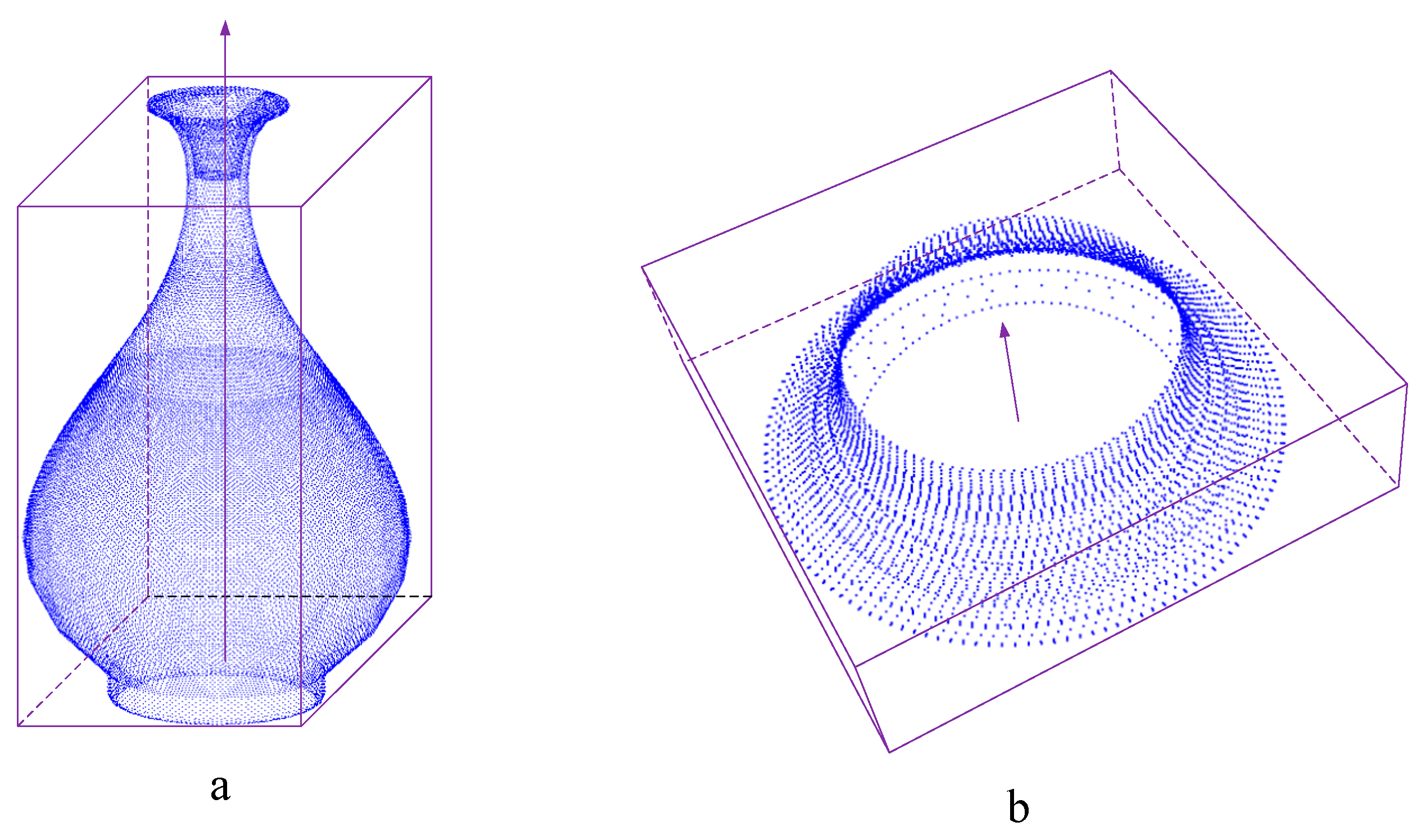
The purpose of extracting the rotation axis of a SOR is to further extract the corresponding projection profile in Step 2. Generally, there are three axial directions parallel to the three sides of oriented bounding box (OBB), whose main axial direction is extracted by the longest side of OBB [26]. However, there are two kinds of SORs—tall-thin type and short-wide type. For tall-thin type SORs as shown in Figure 2a, the acquired axial direction is right by the longest side of OBB, but the wrong axial direction for short-wide type SORs, as shown in Figure 2b. Therefore, aiming to resolve the above issue, we propose a self-adaptive method to extract the rotation axis of a SOR by a minimum relative deviation among the three axial directions of OBB for both tall-thin type and short-wide type SORs after quaternion rotation.

2.1.1. Quaternion Rotation

With the advantage of avoiding gimbal locking, a quaternion can be used to perform arbitrary vector rotation through the origin, which is more convenient and efficient than rotation matrix and rotation vector. Therefore, in this study, the quaternion rotation is used to rotate the extracted axial directions to the Z-axis so that SORs can be in the 3D space along the Z-axis. Generally, any arbitrary quaternion rotation can be completed by only one rotation axis and one rotation angle in the space [16]. Therefore, we denote $n=\left[a,b,c\right]$ as the normalized axial direction of OBB. Thus, the rotation angle $\theta$, between $n$ and Z-axis, can be calculated by Equation (1).

$$\theta =\arccos (n\cdot n_1)$$

(1)

The normalized rotation axis $d$ is calculated by Equation (2)

$$d=n\times n_1$$

(2)

where, $n_1={\left[0,0,1\right]}^{\wedge }T$ is the unit normal vector of Z-axis.

The whole rotational process can be realized by Equation (3).

$$P_1=\mu P{\mu }^{-1}$$

(3)

$$\mu =\cos \frac{\theta }{2}+d\sin \frac{\theta }{2}$$

(4)

$${\mu }^{-1}=\cos \frac{\theta }{2}-d\sin \frac{\theta }{2}$$

(5)

where $P$ denotes the original point clouds, $P_1$ denotes the rotated point clouds.

2.1.2. Extraction of Rotation Axis

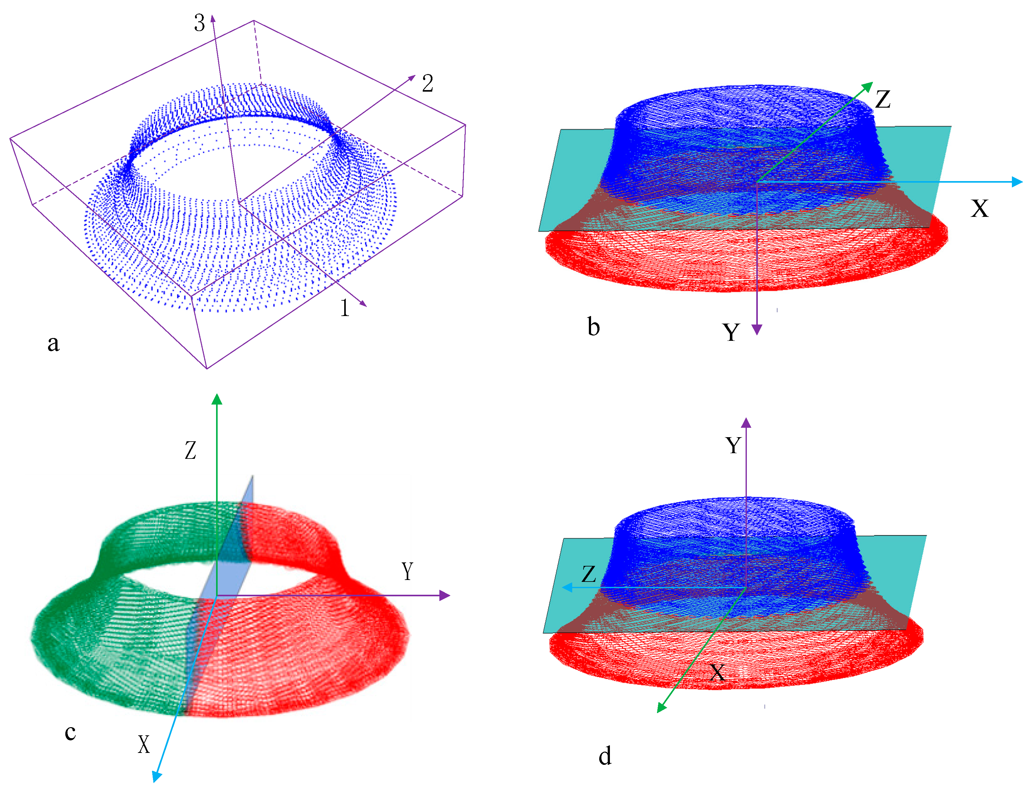
In this study, according to three different axial directions of OBB, as shown in Figure 3, three different coordinate systems can be built, the origin of which is the center of OBB. For any SOR, it must be symmetrical to a plane. Therefore, after quaternion rotation for the three axial directions of OBB, the right rotation axis can be determined by the minimum relative deviation between the two parts of the point cloud, which are divided by the plane that cross the origin and contain the Z-axis. In this study, aiming to improve the efficiency of extraction of rotation axis, the plane $Y=0$ for each coordinate system is used to divide the point cloud into two parts. The detailed algorithm is shown as follows.

(1) Denote $M$ as the number of points in the point cloud, and further divide the point cloud into two parts by the plane $Y=0$.

(2) Denote $N$ as the number of points in the point cloud meeting the condition of $Y>0$, and $M-N$ as the number of points in the point cloud meeting the condition of $Y\le 0$.

(3) The relative deviation $\sigma$ is calculated by $\sigma =\left|M/N-2\right|$ to evaluate the distribution of the divided two-part point clouds.

(4) The axial direction with a minimum relative deviation $\sigma$ is the right axial direction to obtain right rotation axis from the three axial directions.

(5) At last, the rotation axis is extracted by the improved iterative method to obtain rotation axis [15,27].

Figure 3 shows an example of rotation axis extraction for a straw-hat, which is a short-wide type SOR. The point cloud is divided into two parts by the plane $Y=0$ according to axial directions 1, 2, and 3 shown in Figure 3a.

Table 1. Relative deviations of the three rotation axes from axial directions 1, 2, and 3 after quaternion rotation.

Axial Direction	Number of Points M	Number of Points N	Number of Points M-N	Relative Deviation
1	21,668	15,620	6048	0.613
2	21,668	10,966	10,702	0.02
3	21,668	6043	15,625	1.586

shows the relative deviations of the three rotation axes from axial directions 1, 2, and 3 after quaternion rotation. For axial direction 2, the acquired relative deviation is 0.02, which is far less than 0.613 and 1.586 for axial directions 1 and 3, respectively. Thus, we can get the right rotation axis from axial direction 2. Moreover, as shown in Figure 3b,d, the two parts of the point cloud are similar, which are divided by the plane $Y=0$. However, due to the different positive direction of the Y axis, the number of points in the corresponding above and below parts is different between the results according to axial direction 1 and axial direction 3, respectively. For example, the number of the top part $M-N$ of the point cloud is obtained by meeting the condition of $Y\le 0$ according to axial direction 1 as shown in Table 1, but the number of top part $N$ of the point cloud is obtained by meeting the condition of $Y>0$ according to axial direction 3, as shown in Table 1.

2.2. Extraction of Projection Profile

The purpose of the extraction of projection profile is to further extract the point set of the generatrix line of SORs in Step 3. Aiming to improve the efficiency of SORs reconstruction, we propose to extract the projection profile of a SOR by the TIN model and RANSAC algorithm, which is shown as follows.

Denote the projection plane of a SOR as Equation (6).

$$Ax+By+Cz+D=0$$

(6)

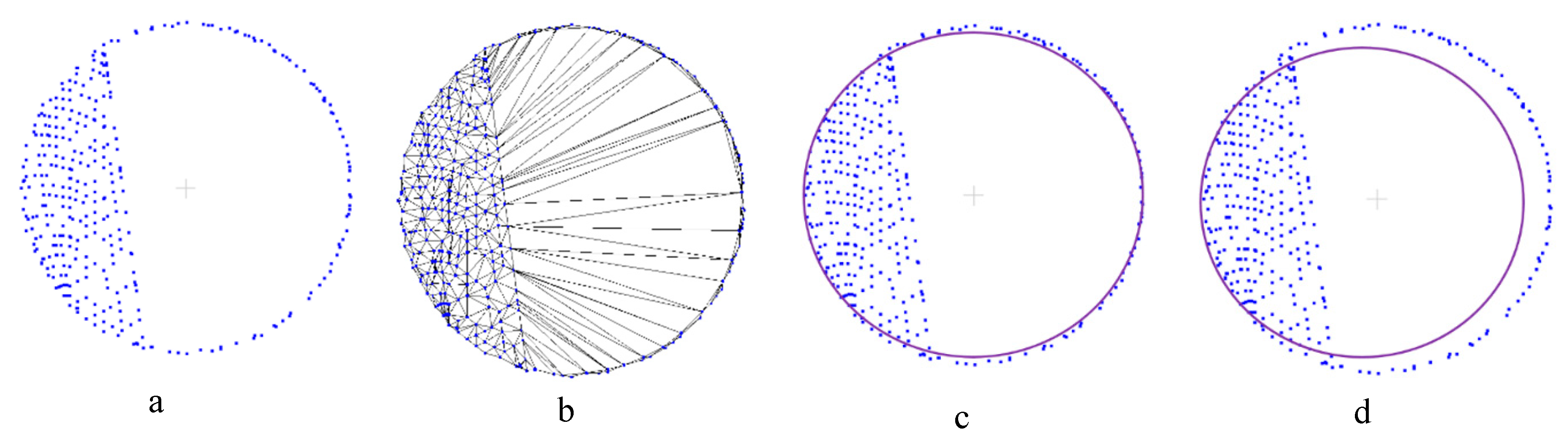
where, (A, B, C) are the normal of the projection plane, and D is the distance from the original point to the projection plane. It is generally known that at least three points on the projection plane are needed to determine the equation of the projection plane. The algorithm of determining the three points are shown as follows: (1) Determine the center of the top and bottom of the model expressed as $P_1\left(a_1,b_1,c_1\right)$ and $P_2\left(a_2,b_2,c_2\right)$, which are calculated accurately by the following algorithm: (1) Traverse the point cloud to seek the maximum and minimum value of coordinate Z, and then determine the point sets on the top and bottom with a preset threshold of 1.5 $f$ ($f$ is the resolution of the used TLS); and (2) As the obtained point sets of the top and bottom usually contain some internal points, if the RANSAC algorithm is directly used to fit the circular contour, the internal point will be used, which will fit the wrong circular contour. Therefore, in this study, the TIN model is firstly constructed based on the above point sets. If there is an edge belonging to only one triangle, this edge must be a boundary of which the two endpoints must be accurate boundary points. Then, the RANSAC algorithm is applied to fit the circular contour to obtain the center of the top and bottom of the model. Figure 4a shows a point set of the top of a straw-hat. Figure 4b is the constructed TIN model. Figure 4c is the fitted circular contour of the top by the proposed method in the paper, which is better than the fitted circular contour by RANSAC algorithm directly as shown in Figure 4d. (2) As the outliers of the point cloud have been removed by using the KD tree neighborhood search algorithm, the model just needs any point on the point cloud to determine the projection plane together with the accurate center of the top and bottom of the model. In this study, aiming to improve the efficiency of extraction of projection profile, a point near to the center of bottom of the model is selected as the third point, which is expressed as $P_3\left(a_2+1,b_2,c_2+1\right)$.

According to the obtained three points on the projection plan, the parameters of Equation (6) A, B, and C can be calculated by Equation (7), and parameter D can be obtained by Equation (8).

$$\left(A,B,C\right)=\left(P_3-P_2\right)\times \left(P_1-P_2\right)$$

(7)

$$D=-\left(A,B,C\right)\cdot P_1$$

(8)

The distance $d$ from each point $\left(x,y,z\right)$ to the projection plane is calculated by Equation (9).

$$d=\left(A,B,C,D\right)\cdot \left(x,y,z,1\right)$$

(9)

At last, the corresponding projection point $p$ can be expressed by Equation (10).

$$p=\left(x,y,z,1\right)-\left(A,B,C,0\right)\times d$$

(10)

In this study, aiming to improve the efficiency of extraction of projection profile, the projection plane of a SOR is defined parallel to the XOZ plane, of which normal A and C are 0. Therefore, the corresponding projection point $p$ can be expressed by Equation (11).

$$p=\left(x,y,z,1\right)-\left(0,B,0,0\right)\times d$$

(11)

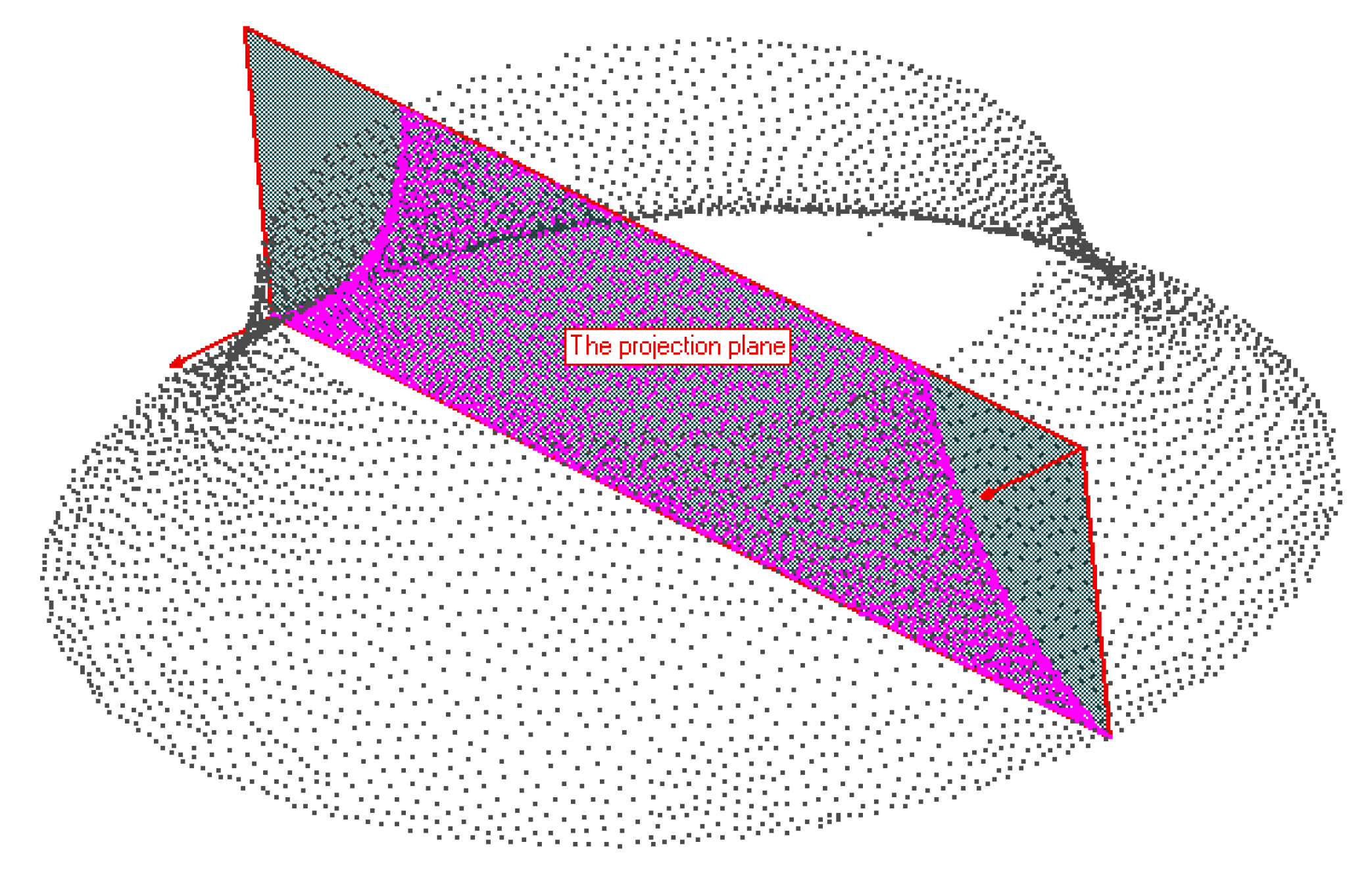
Take the point cloud of a straw hat as an example. By traversing the point cloud to obtain the corresponding projection points, the extracted projection profile of a straw hat is shown in Figure 5.

2.3. Extraction of the Generatrix Line of SORs

2.3.1. Extraction of the Point Set of Boundary X

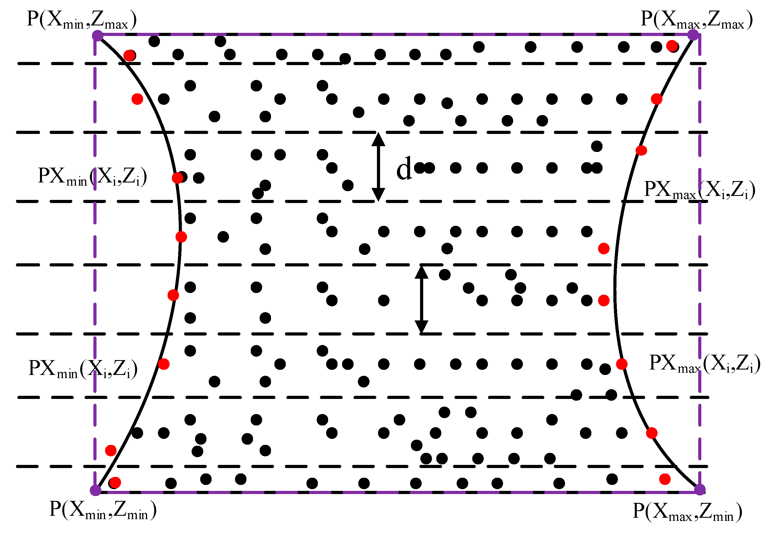
Aiming to extract the point set of the generatrix line of SORs, the point set of boundary X (boundary of projection profile) is determined by searching for coordinate Z with a moving step length $d$, which is calculated by Equation (12).

$$d=\frac{\left(Z_{\max }-Z_{\min }\right)}{\sqrt{n-1}}$$

(12)

where, $Z_{\max }$ and $Z_{\min }$ are the maximum and minimize value of coordinate Z, and n is the number of the points in the point cloud. The schematic diagram of the implementation process is shown in Figure 6. The specific process is shown as follows: (1) Traverse the projected points to obtain the extreme value of coordinate Z, including the minimum value of $P(X_i,Z_{\min })$ and the maximum value of $P(X_j,Z_{\max })$. (2) Let point $P(X_i,Z_{\min })$ be the starting point to search for the two extreme values of coordinate X, the minimum value of $P\left(X_{\min },Z_i\right)$, and the maximum value of $P\left(X_{\max },Z_i\right)$ within the range from $\left(Z_{\min }-d/2\right)$ to $\left(Z_{\min }+d/2\right)$. (3) Coordinate Z is added by a step $d$, and then step (2) is repeated until the coordinate Z is $\left(Z_{\max }+d/2\right)$ acquired for all of the extreme values of coordinate X within the range. (4) Obtain the point set of boundary X of the projection profile by connecting the extreme points of coordinate X. As shown in Figure 6, the point set of boundary X of the projection profile consists of the red points.

2.3.2. Extraction of the Point Set of the Generatrix Line of SORs

As irregularity of the projected point clouds and errors inevitably exist, it is hard to avoid the errors of overflow points (duplication of boundary points) for the above extracted point set of boundary X of the projection profile. Therefore, in the paper, the neighborhood search method is adopted to remove overflow points for the point set of boundary X to extract the point set of the generatrix line. Denote $f$ as the resolution of the point clouds, which is equal to the resolution of the used TLS, and $R$ is the radius of the neighborhood search ($R=1.1f$). If the number of points in the neighborhood is 0, then delete the point, otherwise, retain the point. Figure 7a shows an extracted point set of boundary X containing overflow points for a straw hat, and Figure 7b shows the processed point set of boundary X without overflow points, which is the acquired point set of the generatrix line.

2.3.3. Generatrix Line Fitting

Generally, the generatrix line of a SOR is a curve. However, for some special SORs, such as a cone, a conical frustum, and a cylinder, the corresponding generatrix line is straight. Therefore, aiming to improve the efficiency of automatic SORs reconstruction, we propose a self-adaptive method to determine the type of generatrix line. The acquired point set of the generatrix line is first made by linear fitting with the total least squares method and curve fitting by the quadratic curve fitting method, respectively [27,28,29]. Then, the type of the generatrix line is determined by choosing the method corresponding to smaller RMS errors. At last, the entity model of SORs is constructed by the solid geometry (CSG) method based on the extracted rotation axis and the fitted generatrix line. The quadratic curve fitting method is described as follows.

Define the implicit equation of the quadratic curve by Equation (13).

$$Q\left(x,y\right)=A{x}^2+Bxy+C{y}^2+Dx+Ey+F=0$$

(13)

where, $A,B,C,D,E,F$ are the coefficients of the quadratic curve. Denote function $I={\displaystyle \sum _{i=1}^{n}Q{\left(x,y\right)}^2}$ and obtain the minimum value $I_{\min }$ from all discrete points in the plane $\left(x_i,y_i\right)\left(i=1,2,3\dots n\right)$. Then, we can obtain the following results, shown as Equation (14).

$$\{\begin{array}{l}2{\displaystyle \sum _{i=1}^{n}Q\left(x,y\right)}{x}^2=0\\ 2{\displaystyle \sum _{i=1}^{n}Q\left(x,y\right)}xy=0\\ 2{\displaystyle \sum _{i=1}^{n}Q\left(x,y\right)}{y}^2=0\\ 2{\displaystyle \sum _{i=1}^{n}Q\left(x,y\right)}x=0\\ 2{\displaystyle \sum _{i=1}^{n}Q\left(x,y\right)}y=0\\ 2{\displaystyle \sum _{i=1}^{n}Q\left(x,y\right)}=0\end{array}$$

(14)

For the above homogeneous equations, it is clear that only zero solution satisfies them, i.e., $A=B=C=D=E=F=0$. Furthermore, in order to obtain an effective solution, a hypothetical condition of variable $A=1.0$ is added to get a new solution, shown as Equation (15).

$$x_1=\left[A_1{ \mathrm{B}}_1{ \mathrm{C}}_1{ \mathrm{D}}_1{ \mathrm{E}}_{1 }{ \mathrm{F}}_1\right], \mathrm{where} A_1=1.0$$

(15)

Using the same method, B, C, D, E, and F are supposed to be 1.0 to obtain the following five groups of solutions.

$$x_2=\left[A_2{ \mathrm{B}}_2{ \mathrm{C}}_2{ \mathrm{D}}_2{ \mathrm{E}}_{2 }{ \mathrm{F}}_2\right], \mathrm{Where} B_2=1.0$$

(16)

$$x_3=\left[A_3{ \mathrm{B}}_3{ \mathrm{C}}_3{ \mathrm{D}}_3{ \mathrm{E}}_{3 }{ \mathrm{F}}_3\right], \mathrm{Where} C_3=1.0$$

(17)

$$x_4=\left[A_4{ \mathrm{B}}_4{ \mathrm{C}}_4{ \mathrm{D}}_4{ \mathrm{E}}_4{ \mathrm{F}}_4\right], \mathrm{Where} D_4=1.0$$

(18)

$$x_5=\left[A_5{ \mathrm{B}}_5{ \mathrm{C}}_5{ \mathrm{D}}_5{ \mathrm{E}}_5{ \mathrm{F}}_5\right], \mathrm{Where} E_5=1.0$$

(19)

$$x_6=\left[A_6{ \mathrm{B}}_6{ \mathrm{C}}_6{ \mathrm{D}}_6{ \mathrm{E}}_6{ \mathrm{F}}_6\right], \mathrm{Where} F_6=1.0$$

(20)

In order to avoid a bigger error caused by the single solution, a linear combination is defined from the six groups of solutions, shown as Equation (21).

$$I_i={\displaystyle \sum _{j=1}^n{(A_i{x}_j^2+B_i{x}_j{y}_j+C_i{y}_j^2+D_i{x}_j+E_i{y}_j+F_i)}^2}(i=1,2,3\cdots 6)$$

(21)

Furthermore, combination coefficients ${\alpha }_i(i=1,2,3,4,5)$ can be determined by Equation (22).

$$S={\left[{\displaystyle \sum _{i=1}^5{\alpha }_i}{I}_i+\left(1-{\alpha }_1-{\alpha }_2-{\alpha }_3-{\alpha }_4-{\alpha }_5\right)I_6\right]}^2$$

(22)

In order to obtain the minimum value of S, Equation (23) is founded.

$$\{\begin{array}{l}\frac{\partial S}{\partial {\alpha }_1}=0\\ \frac{\partial S}{\partial {\alpha }_2}=0\\ \frac{\partial S}{\partial {\alpha }_3}=0\\ \frac{\partial S}{\partial {\alpha }_4}=0\\ \frac{\partial S}{\partial {\alpha }_5}=0\end{array}$$

(23)

Equation (23) is further expanded to acquire nonhomogeneous linear equations, shown as Equation (24).

$$\{\begin{array}{l}(I_1-I_6)((I_1-I_6){\alpha }_1+(I_2-I_6){\alpha }_2+(I_3-I_6){\alpha }_3+(I_4-I_6){\alpha }_4+(I_5-I_6){\alpha }_5)=I_6(I_6-I_1)\\ (I_2-I_6)((I_1-I_6){\alpha }_1+(I_2-I_6){\alpha }_2+(I_3-I_6){\alpha }_3+(I_4-I_6){\alpha }_4+(I_5-I_6){\alpha }_5)=I_6(I_6-I_2)\\ (I_3-I_6)((I_1-I_6){\alpha }_1+(I_2-I_6){\alpha }_2+(I_3-I_6){\alpha }_3+(I_4-I_6){\alpha }_4+(I_5-I_6){\alpha }_5)=I_6(I_6-I_3)\\ (I_4-I_6)((I_1-I_6){\alpha }_1+(I_2-I_6){\alpha }_2+(I_3-I_6){\alpha }_3+(I_4-I_6){\alpha }_4+(I_5-I_6){\alpha }_5)=I_6(I_6-I_4)\\ (I_5-I_6)((I_1-I_6){\alpha }_1+(I_2-I_6){\alpha }_2+(I_3-I_6){\alpha }_3+(I_4-I_6){\alpha }_4+(I_5-I_6){\alpha }_5)=I_6(I_6-I_5)\end{array}$$

(24)

According to Equation (24), the value of ${\alpha }_i(i=1,2,3,4,5)$ can be obtained. Furthermore, let ${\alpha }_6=1-{\displaystyle \sum _{i=1}^5{\alpha }_i}$, the coefficients $A,B,C,D,E,F$ of the quadratic curve can be obtained, which are shown as Equation (25).

$$\begin{array}{ccc}A={\displaystyle \sum _{i=1}^6{\alpha }_i{A}_i}& B={\displaystyle \sum _{i=1}^6{\alpha }_i{B}_i}& C={\displaystyle \sum _{i=1}^6{\alpha }_i{C}_i}\\ D={\displaystyle \sum _{i=1}^6{\alpha }_i{D}_i}& E={\displaystyle \sum _{i=1}^6{\alpha }_i{E}_i}& F={\displaystyle \sum _{i=1}^6{\alpha }_i{F}_i}\end{array}$$

(25)

3. Experiments and Analysis

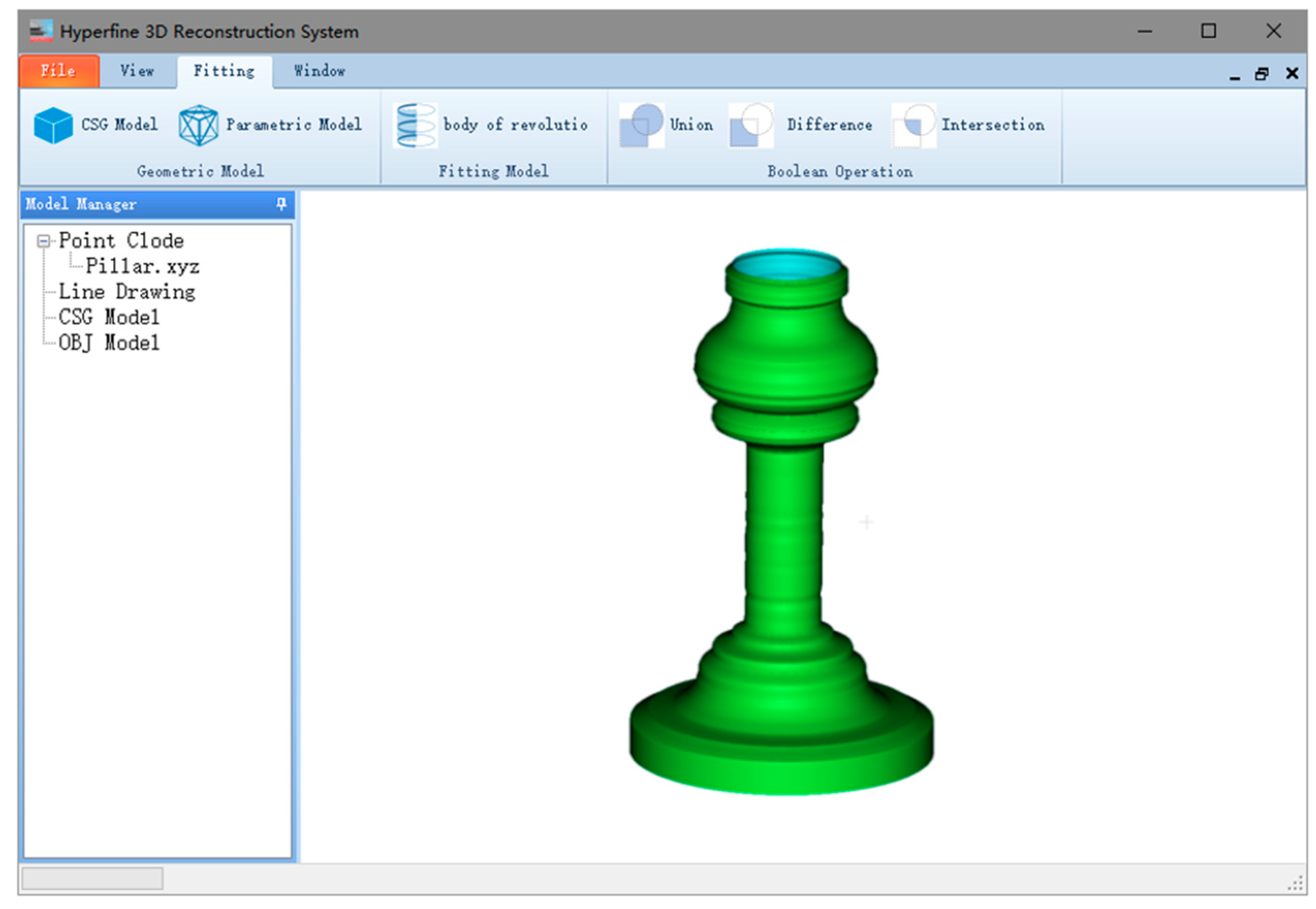
In order to validate the efficiency and accuracy of the proposed method, the reconstructed SORs of the geometric objects by the use of the proposed method are firstly compared with the curvature computation method [24], and then compared with other surface reconstruction methods, including the Delaunay-based method [30], the Poisson method [31], and the radial basis function (RBF) method [32], respectively. All of the above point clouds for the experimental SORs are acquired by a Z+F Imager 5016 scanner, of which the measurement accuracy is better than 1 mm with a measuring distance of less than 50 m. In the paper, the point cloud processing for SORs reconstruction and results analysis are both performed by the use of 3D Spatial Data Hyperfine Modeling System as shown in Figure 8, which is developed by Beijing University of Civil Engineering and Architecture.

3.1. Comparison with the Curvature Computation Method

In this study, three kinds of SORs, simple SORs with a generatrix line of a straight line, tall-thin SORs, and short-wide SORs with a generatrix line of a curve are selected to make a comparison between the curvature computation method and the proposed method.

3.1.1. Simple SORs

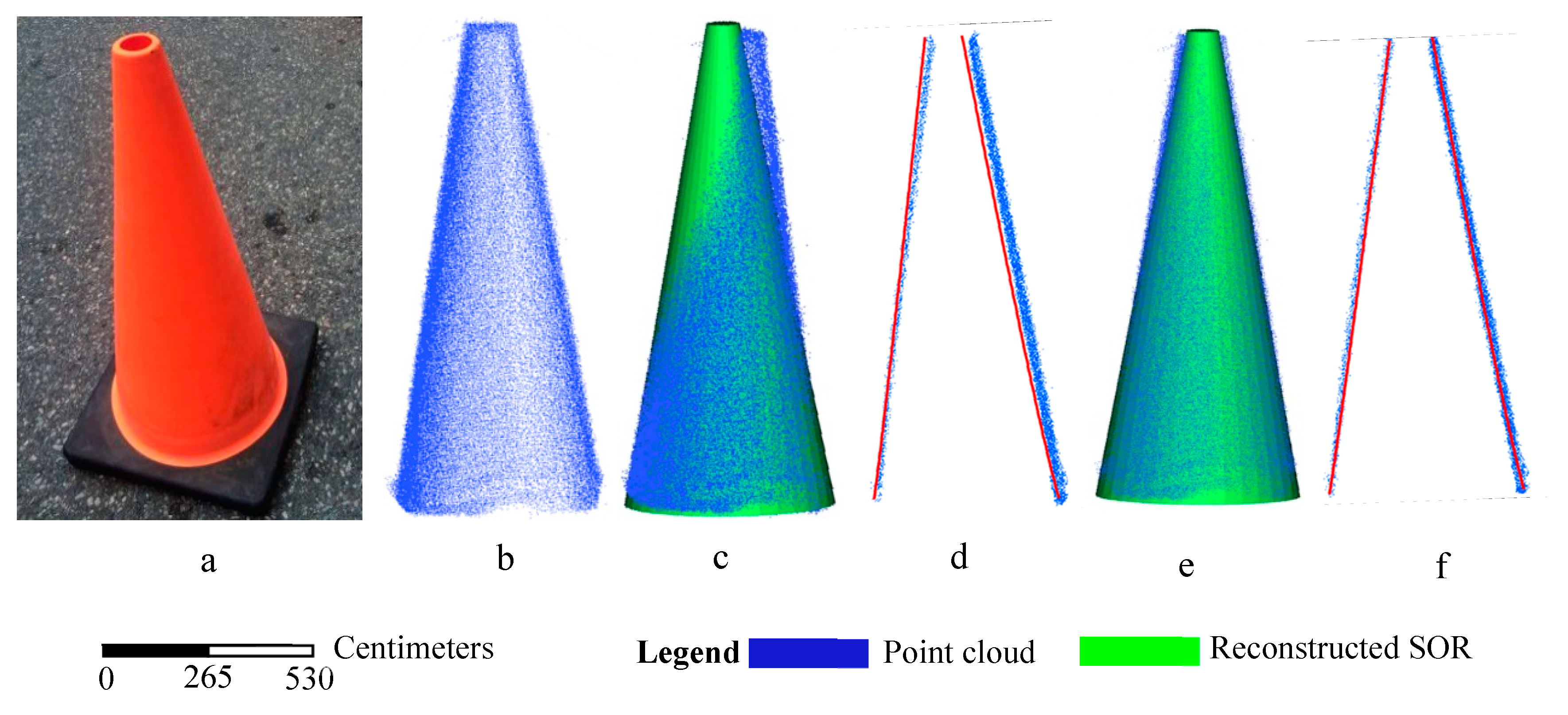
Two kinds of simple SORs, a cylinder and a frustum of a cone, are selected for comparison. Figure 9b shows a point cloud of a cylinder with 148,400 points, which is a section of big timber construction in the Imperial Palace shown in Figure 9a. Figure 10a shows a point cloud of a frustum of a cone (which is a traffic cone) with 89,528 points.

Considering the effects of the irregularity and errors of the acquired point clouds, overflow points processing and the total least squares method are adopted during the process of extraction of the generatrix line, which can improve the accuracy of the acquired point set of the generatrix line. As shown in Figure 9 and Figure 10, the reconstructed SORs by the proposed method have a much better compactness than that of the curvature computation method. In order to evaluate the accuracy of the reconstructed SORs, the RMS error of each reconstructed SOR is calculated. For the reconstructed SOR of a cylinder, as shown in

Table 2. Parameters comparison for the two reconstructed simple SORs between the curvature computation method and the proposed method.

Objects	Parameters	Curvature Computation Method	Proposed Method	Percentage Improvement
Cylinder	RMS (mm)	0.42	0.29	30.1%
	Time (ms)	2151	1039	51.7%
Frustum of a cone	RMS (mm)	0.56	0.29	41.1%
	Time (ms)	1928	1001	48.1%

, the RMS error of the reconstructed SOR of the cylinder is 0.29 mm, which is much better than 0.42 mm obtained by the curvature computation method. The percentage improvement of accuracy is 30.1%. For the reconstructed SOR of a frustum of a cone, as shown in Table 2, the RMS error of the reconstructed SOR of the frustum of a cone is 0.29 mm, which is much better than 0.56 mm obtained by the curvature computation method. The percentage improvement of accuracy is 41.1%, which is much more than that of the reconstructed SOR of the cylinder. Moreover, as shown in Figure 10c,d, the reconstructed SOR of the frustum of a cone by the curvature computation method deviates from the position of the corresponding point cloud, especially for the upper part of the reconstructed SOR. The reason is that there are some overflow points in the point cloud of the frustum of a cone. This indicates that the proposed method has a higher denoising performance. Furthermore, without the requirement of calculating the normal vectors of point clouds, the proposed method’s efficiency is greatly improved. As shown in Table 2, for the two kinds of simple SORs, the time efficiency is increased by about 50%.

3.1.2. Tall-Thin SORs

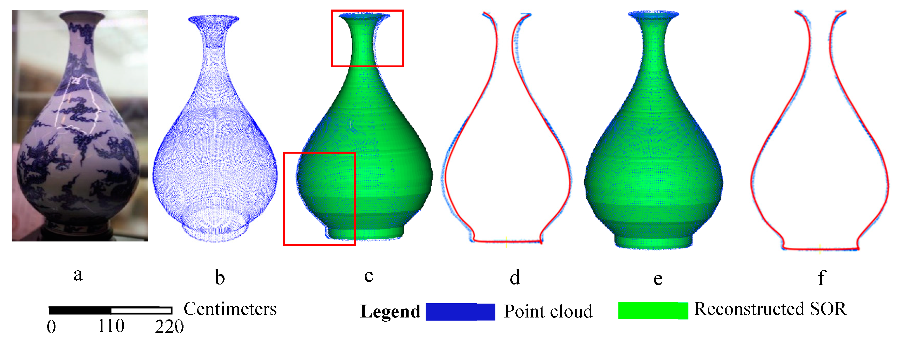
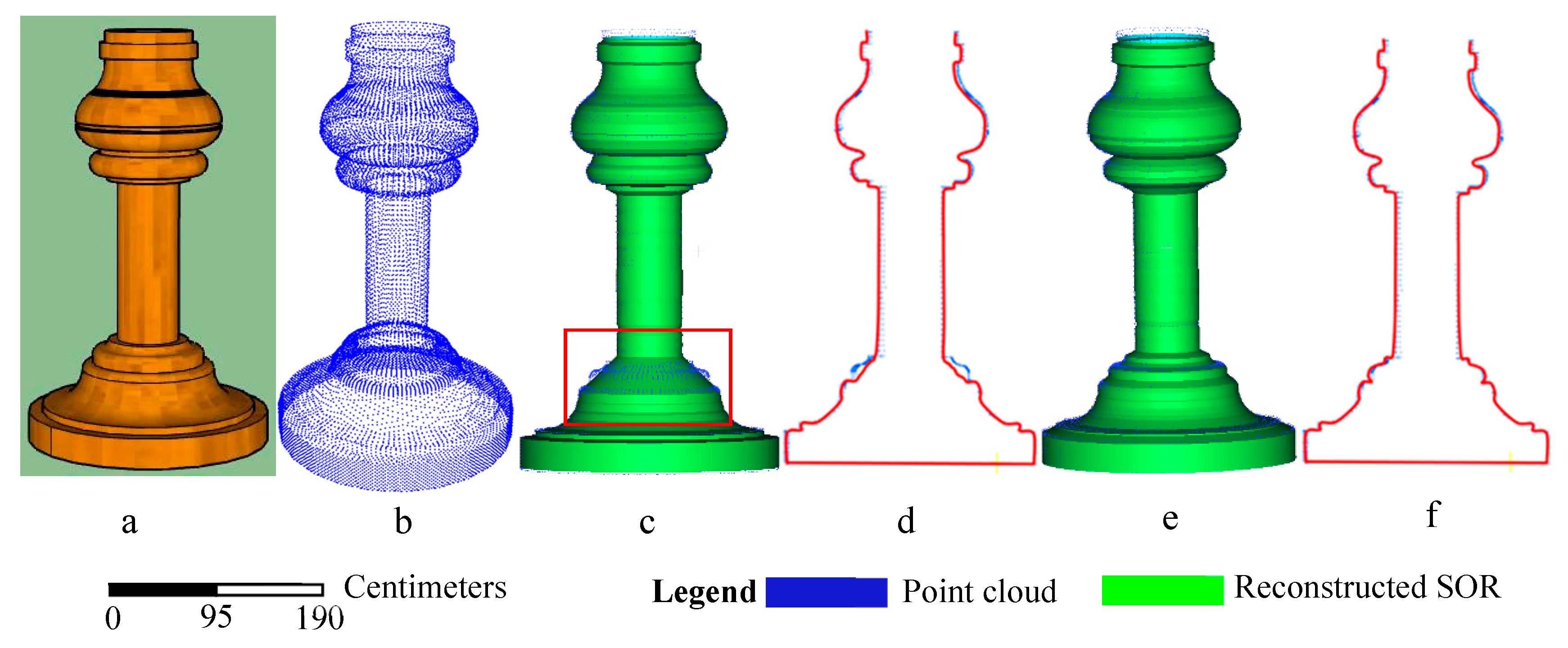
Two tall-thin SORs are selected as the experimental objects in this paper; one is a point cloud of a vase in the Imperial Palace with 36,114 points, as shown in Figure 11a,b, and the other is a point cloud of a pillar of an ancient building in the Imperial Palace with 20,697 points, as shown in Figure 12a,b. Like the reconstructed simple SORs, by using the proposed method, the RMS errors of the two reconstructed tall-thin SORs are much better than that of the curvature computation method, as shown in

Table 3. Parameters comparison for the two reconstructed tall-thin SORs between the curvature computation method and the proposed method.

Objects	Parameters	Curvature Computation Method	Proposed Method	Percentage Improvement
Vase	RMS (mm)	0.35	0.24	31.4%
	Time (ms)	2450	1835	25.1%
Pillar	RMS (mm)	0.43	0.30	30.2%
	Time (ms)	1836	1349	26.5%

. For the reconstructed SOR of a vase, the RMS error of the reconstructed SOR of the cylinder is 0.24 mm, which is much better than 0.35 mm obtained by the curvature computation method, and the accuracy of percentage improvement is 31.4%. For the reconstructed SOR of a pillar, the RMS error of the reconstructed SOR of the cylinder is 0.30 mm, which is much better than 0.43 mm obtained by the curvature computation method, and the percentage improvement of accuracy is 30.2%. Especially for the area shown in red rectangles in Figure 11c and Figure 12c, there are some deviations between the original point cloud and the reconstructed SORs. Therefore, the tall-thin SORs reconstructed by the proposed method have a much better compactness compared with the curvature computation method, which is shown in Figure 11 and Figure 12. The efficiency is also greatly improved for the reconstructed tall-thin SORs by the proposed method. As shown in Table 3, the percentage improvement of time efficiency is 25.1% and 26.5% for the reconstructed tall-thin SORs of a vase and a pillar, respectively, which are lower than that of the simple SORs with a straight generatrix line. This indicates that the proposed method is more efficient for simple SORs with a straight generatrix line.

3.1.3. Short-Wide SORs

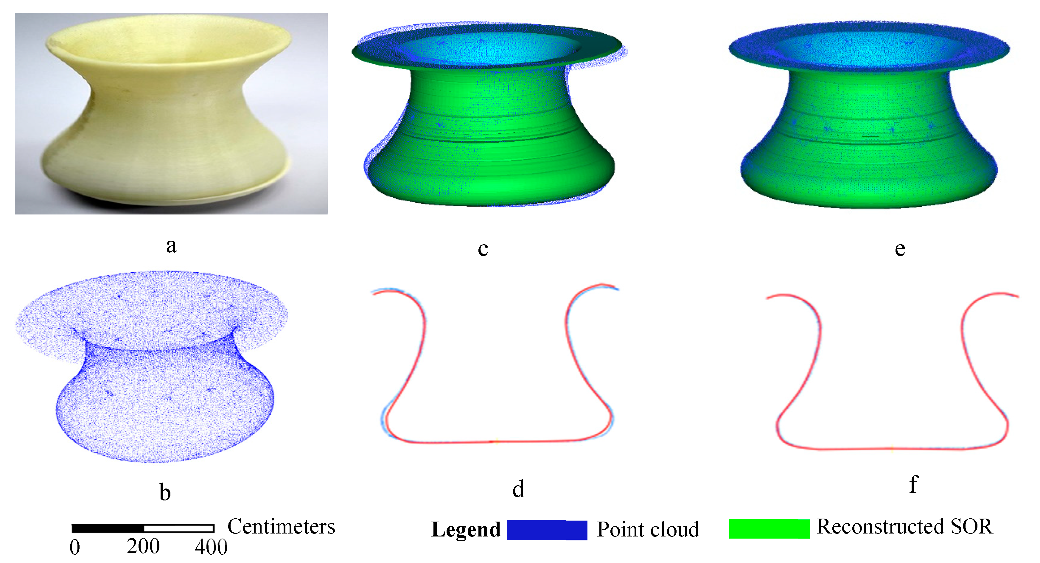
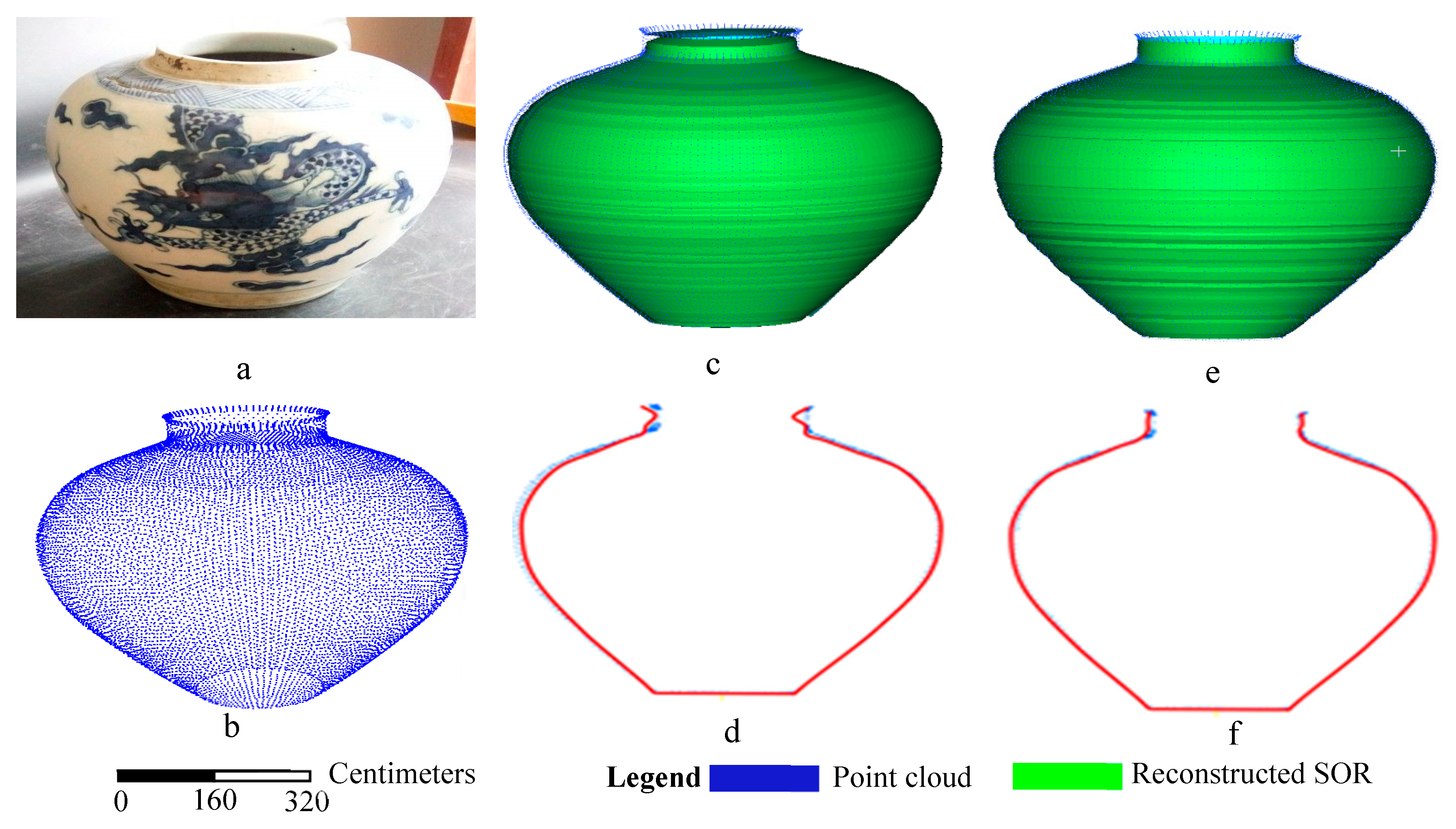
Two short-wide SORs are selected as the experimental objects; one is a point cloud of a pot in the Imperial Palace with 49,673 points, as shown in Figure 13a,b, and the other is a point cloud of a ceramic in the Imperial Palace with 15,783 points, as shown in Figure 14a,b. Like the tall-thin SORs reconstructed by the proposed method, the RMS errors of the two short-wide SORs are also much better than that of the curvature computation method, as shown in

Table 4. Parameters comparison for the two reconstructed short-wide SORs between the curvature computation method and the proposed method.

Objects	Parameters	Curvature Computation Method	Proposed Method	Percentage Improvement
Pot	RMS (mm)	0.51	0.21	58.8%
	Time (ms)	4020	3012	25.1%
Ceramic	RMS (mm)	0.33	0.23	30.3%
	Time (ms)	1548	1113	28.1%

. Especially for the reconstructed SOR of a pot, the percentage improvement of accuracy is up to 58.8%. Obviously, as shown in Figure 13c, it is a sloping reconstructed SOR compared with the original point cloud, which is caused by the poor quality of the acquired normal of the point cloud of the pot by the curvature computation method. The efficiency is also greatly improved for the reconstructed short-wide SORs by use of the proposed method. As shown in Table 4, the percentage improvement of time efficiency is 25.1% and 28.1% for the reconstructed short-wide SORs of a pot and a ceramic, respectively, which is similar to reconstructed tall-thin SORs. This indicates that the percentage improvement of time efficiency is almost identical for both tall-thin SORs and short-wide SORs by the proposed method.

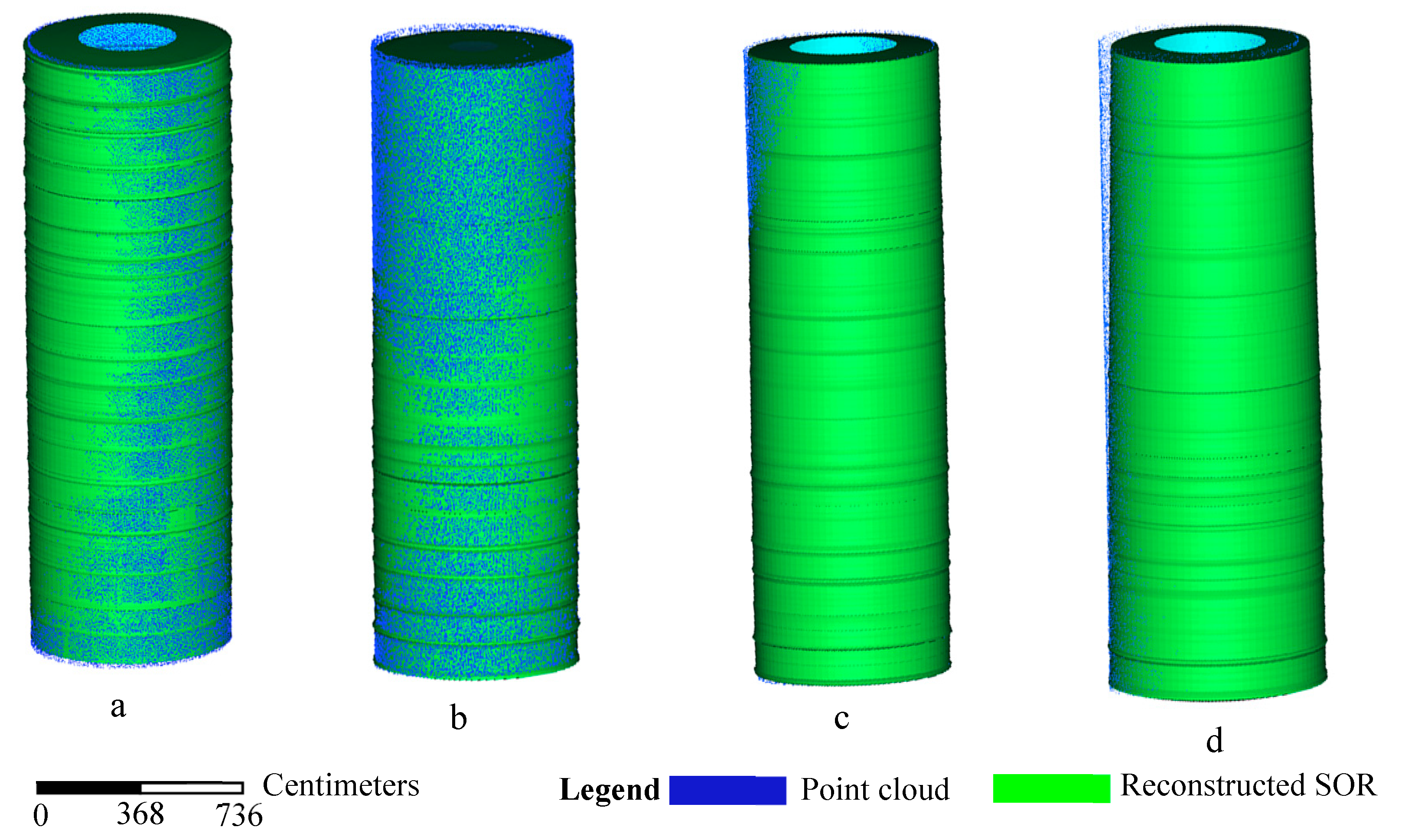
3.2. Comparison with Surface Reconstruction Methods

A pillar of an ancient building was selected to compare the Delaunay-based method, the Poisson method, the RBF method, and the proposed method. The point cloud is shown in Figure 12b. The reconstructed surfaces by the above four methods are shown in Figure 15. The inspection from this figure highlights that: (1) As the reconstructed triangular facets are made through each point by the Delaunay-based method, it has a minimum RMS error of 0.06 mm among the four surface reconstruction methods. However, with the influence of the quality of the point cloud, as shown in Figure 15a, it often produces some holes on the reconstructed surface. Although the surface reconstructed by the Poisson method and the RBF method also have smaller RMS errors (

Table 5. Parameters comparison for the reconstructed SOR of a pillar of an ancient building by the Delaunay-based method, Poisson method, RBF method, and the proposed method.

Parameters	Delaunay	Poisson	RBF	Proposed Method
RMS (mm)	0.06	0.58	0.45	0.30
Time (ms)	1936	1489	1523	1349

), the Poisson method often suffers from a tendency to over-smooth the data. The RBF method is based on the Hermite radial basis function to approximate a surface, which may cause some distortion of the reconstructed surface due to a lack of smoothness, as shown in Figure 15c. Therefore, considering the geometric characteristics of SORs, the proposed method has a higher accuracy of SOR reconstruction and good robustness. (2) As shown in Table 5, the most time efficient method of surface reconstruction is the proposed method.

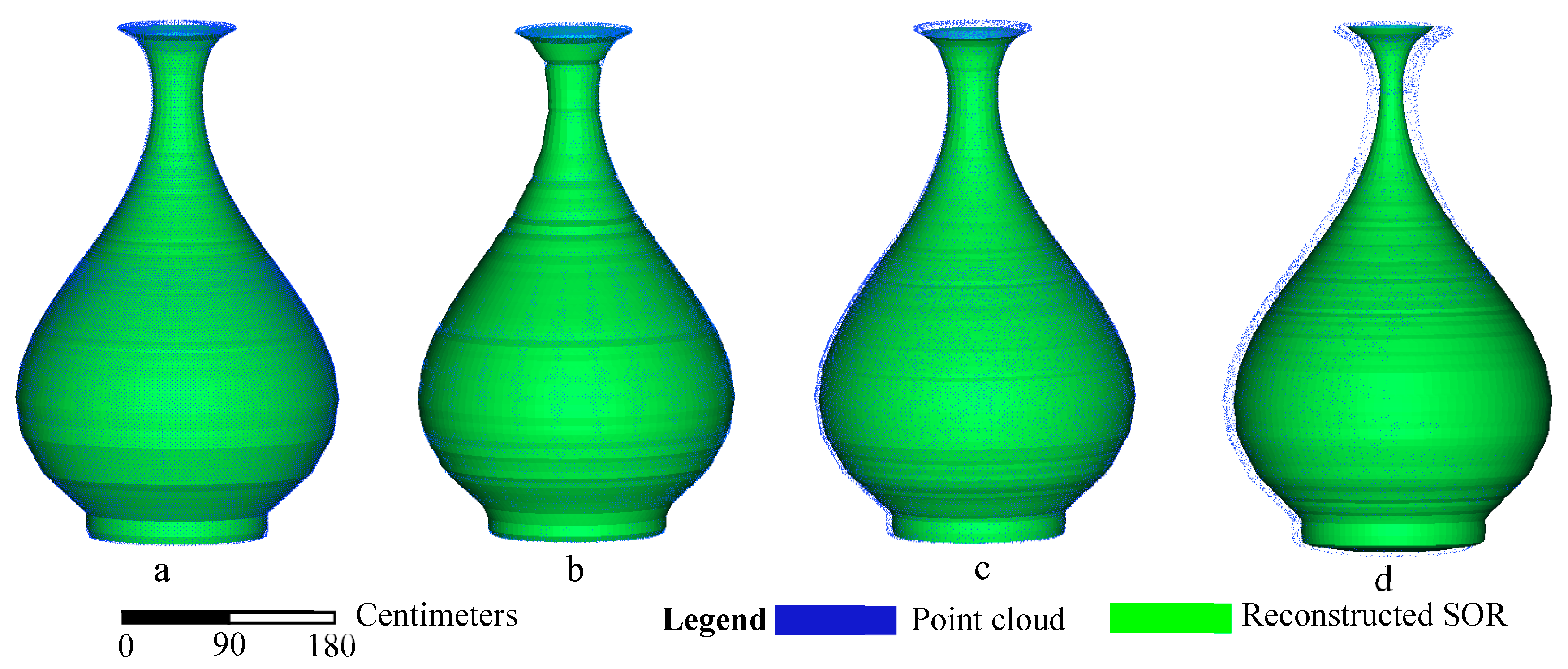
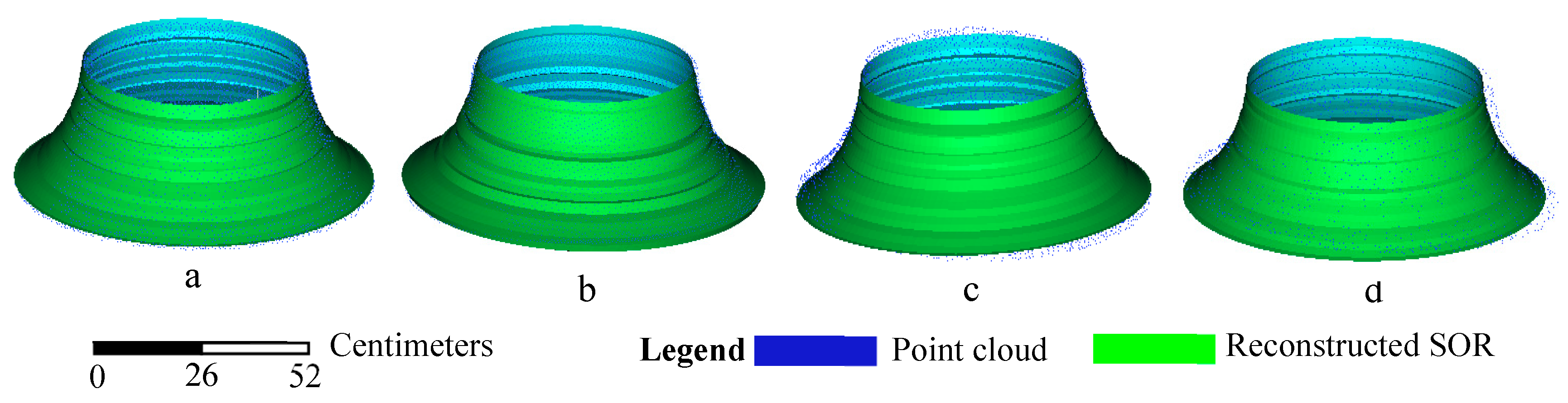
3.3. Accuracy Analysis

To evaluate the reliability of the proposed method, three different types of SORs, including a simple SOR, a tall-thin SOR, and a short-wide SOR, underwent accuracy analysis with different sampling rates of 100%, 75%, 50%, and 25% for the original point clouds by the use of the VoxelGrid filter. The reconstructed SORs for the three different types of SOR with different sampling rates are shown in Figure 16, Figure 17, and Figure 18, respectively. The inspection of the reconstructed SORs clearly highlights that: (1) With decreased sampling rate of point clouds, the accuracy of the reconstructed SORs was also reduced. As shown in

Table 6. Accuracy comparison of the reconstructed SORs with different sampling rates for a simple SOR, a tall-thin SOR, and a short-wide SOR.

	Sampling Rate	100%	75%	50%	25%
Simple SOR	Number of points	148,400	111,300	74,200	37,100
	RMS (mm)	0.28	0.88	3.9	4.5
Tall-thin SOR	Number of points	36,114	27,085	18,057	9028
	RMS (mm)	0.32	0.85	3.77	4.81
Short-wide SOR	Number of points	10,131	7598	5065	2532
	RMS (mm)	0.26	0.81	4.47	5.54

, for the point clouds with a sampling rate of 100% and 75%, the RMS errors of the reconstructed SORs were better than 1 mm for the above three different type SORs. However, for the point clouds with a sampling rate of 50% and 25%, the RMS errors of the reconstructed SORs increased. The reason is that the accuracy of the reconstructed SORs is determined by the accuracy of the obtained generatrix line, which is determined by the sampling interval of the original point clouds. (2) Although different sampling rates of the original point clouds produced different accuracies of the reconstructed SORs, even for the 25% sampling rate, the reconstructed SORs recovered the true shape of the model, which validated the reliability of the proposed method.

4. Discussion

This paper explored an automatic, self-adaptive SOR reconstruction method for generatrix line extraction from point clouds, with the purpose of improving the efficiency and accuracy of SORs reconstruction. Based on the results of the aforementioned experiments, there are three issues that need to be discussed:

(1) As there is no need for calculating the normal of point clouds, by using the proposed method, the RMS errors of all the reconstructed SORs have a consistent accuracy, which was better than 0.3 mm. However, when using the curvature computation method, the quality of the reconstructed SORs is determined by the local surface characteristics and the quality of original point cloud [22], and the corresponding RMS errors range from 0.33 mm to 0.70 mm for the aforementioned experiments. Yang et al. [18] achieved about 1 mm accuracy for radius estimation by dense Simultaneous Localization and Mapping (SLAM). Son et al. [24] achieved a normalized mean error range from 2.74% to 3.68% for seven types of pipelines with radii ranging from 76.2 mm to 304.6 mm by using Leica ScanStation C10, which has an approximately 2 mm spot size at a distance of 10 m in a medium-density scan setup. Therefore, although the proposed method can only reconstruct SORs, it is more robust than the curvature computation method, and ensures consistently high accuracy of the reconstructed SORs. In addition, the proposed SORs reconstruction method was compared with other surface reconstruction methods, including the Delaunay-based method, the Poisson method, and the RBF method. The Delaunay-based method often produces holes in the reconstructed surface [33], the Poisson method often suffers from a tendency to oversmooth the data [34], and the RBF method may cause some distortions on the reconstructed surface [35]. Therefore, considering the geometric characteristics of SORs, the proposed method is robust and has high accuracy and efficiency for SORs reconstruction.

(2) The accuracy of SORs reconstruction is greatly influenced by the sampling rate of the original point cloud. With decreased density of point clouds, the accuracy of the reconstructed SORs also decreases. In this study, four different sampling rates of 100%, 75%, 50%, and 25% of the original point cloud were selected in the accuracy analysis of three different types of SORs. With the decrease of sampling rate of the original point cloud, the accuracy of the reconstructed SORs was reduced greatly. The reason is that a generatrix line of a SOR is extracted from a point set from the extract projection profile. If the density of a point cloud is reduced, there may not be enough points to describe the detail of the generatrix line of a SOR, i.e., the lower the sampling rate of the original point cloud, the fewer points in the point set of the generatrix line of a SOR [36]. Therefore, the quality of SORs reconstruction relates to the density of the original point cloud; meanwhile, more points increase the memory and time consumption [37,38,39].

(3) In this study, the original point cloud contained only one SOR without outliers for automatic SORs reconstruction. However, there are many different types of point clouds, such as a point cloud with mainly one SOR-type surface without outliers, a point cloud containing many SOR-type surface, a point cloud containing only one SOR-type surface, but with other points not belonging to the surface, and a point cloud with mainly one SOR-type surface and a small percentage of outliers [40]. Therefore, if the original point cloud contains many SOR-type surfaces, point cloud segmentation should be performed to extract each SOR-type surface. Also, if the original point cloud contains other points not belonging to the surface and a small percentage of outliers, preprocessing is necessary to ensure the obtained point cloud only contains one SOR-type surface without redundant points and outliers. In this study, the outliers of the point cloud are removed by using the KD tree neighborhood search algorithm, the projection profile of a SOR is extracted by integrating the TIN model and the RANSAC algorithm, and the generatrix line is extracted by the linear fitting method, which improve the robustness the reconstructed SOR.

5. Conclusions

In this paper, an automatic, self-adaptive SOR reconstruction algorithm is proposed to extract the generatrix line of SORs from point clouds. Compared with the curvature computation method, as there is no need to calculate the normal of point clouds nor to set too many thresholds, the efficiency and accuracy of SORs reconstruction is greatly improved. More specifically, the results presented in the paper clearly highlight that:

(1) By the use of OBB, the efficiency of rotation axis extraction of SORs can be greatly improved. In addition, in order to avoid false extraction of the rotation axis of SORs, relative deviation and quaternion rotation are integrated to automatically extract the rotation axis among the three axial directions for both tall-thin and short-wide SORs. Furthermore, by the use of quaternion rotation to rotate the extracted axial directions to the Z-axis, it is easy to extract the projection profile of the point cloud. At the same time, the TIN model and RANSAC algorithm are integrated to extract the projection profile of the SOR, which improves the robustness of the extracted projection profile.

(2) By the use of the proposed method, the reconstructed SORs have consistent accuracy, the RMS errors of which are better than 0.3 mm. Meanwhile, with the advantage of not needing to calculate the normal vectors of point clouds, it can greatly improve the efficiency of SORs reconstruction by the use of extremum searching method with overflow point processing. The type of the generatrix line is automatically determined by taking the smaller RMS error of either linear fitting or quadratic curve fitting. As a result, compared with the curvature computation method, for simple SORs, the efficiency of SORs reconstruction can be increased by more than 50%, and by more than 25% for complex SORs.

(3) With different sampling rate of the original point cloud, even for sampling rate of 25%, the proposed method can still reconstruct the true shape of SORs, which indicates that the proposed method is robust for SORs reconstruction. However, with the decrease of sampling rate of the original point cloud, the accuracy of the reconstructed SORs was also greatly reduced. Therefore, if one wants to obtain a reconstructed SOR with high accuracy, one needs to ensure a high density of the original point cloud.

References

- Hoover, A.; Jean-Baptiste, G.; Jiang, X.; Flynn, P.; Bunke, H.; Goldgof, D.; Bowyer, K.; Eggert, D.; FitzGibbon, A.; Fisher, R. An experimental comparison of range image segmentation algorithms. IEEE Trans. Pattern Anal. Mach. Intell. 1996, 18, 673–689. [Google Scholar] [CrossRef]
- Qian, X.; Huang, X. Reconstruction of surfaces of revolution with partial sampling. J. Comput. Appl. Math. 2004, 163, 211–217. [Google Scholar] [CrossRef]
- Colombo, C.; Del Bimbo, A.; Pernici, F. Metric 3D reconstruction and texture acquisition of surfaces of revolution from a single uncalibrated view. IEEE Trans. Pattern Anal. Mach. Intell. 2005, 27, 99–114. [Google Scholar] [CrossRef]
- Alcázar, J.G.; Goldman, R. Finding the axis of revolution of an algebraic surface of revolution. IEEE Trans. Vis. Comput. Graph. 2016, 22, 2082–2093. [Google Scholar] [CrossRef]
- Weisstein, E.W. Surface of Revolution. From MathWorld--A Wolfram Web Resource. Available online: http://mathworld.wolfram.com/SurfaceofRevolution.html (accessed on 1 April 2019).
- Kang, Z.; Zhang, L.; Wang, B.; Li, Z.; Jia, F. An Optimized BaySAC Algorithm for Efficient Fitting of Primitives in Point Clouds. IEEE Geosci. Sens. Lett. 2014, 11, 1096–1100. [Google Scholar] [CrossRef]
- Alcazar, J.G.; Goldman, R. Detecting When an Implicit Equation or a Rational Parametrization Defines a Conical or Cylindrical Surface, or a Surface of Revolution. IEEE Trans. Vis. Comput. Graph. 2017, 23, 2550–2559. [Google Scholar] [CrossRef] [PubMed]
- Willis, A.R.; Cooper, D.B. Computational reconstruction of ancient artifacts. IEEE Signal Proc. Mag. 2008, 25, 65–83. [Google Scholar] [CrossRef]
- Shi, X.; Goldman, R. Implicitizing rational surfaces of revolution using u-bases. Comput. Aided Geom. Des. 2012, 29, 348–362. [Google Scholar] [CrossRef]
- Vršek, J.; Lávička, M. Determining surfaces of revolution from their implicit equations. J. Comput. Appl. Math. 2015, 290, 125–135. [Google Scholar] [CrossRef]
- Lee, I.-K. Curve reconstruction from unorganized points. Comput. Aided Geom. Des. 2000, 17, 161–177. [Google Scholar] [CrossRef]
- Peternell, M.; Pottmann, H. Approximation in the space of planes: applications to geometric modeling and reverse engineering. Rev. Real Acad. Cienc. Ser. A Math 2002, 96, 243–256. [Google Scholar]
- Xu, Y.; Tuttas, S.; Hoegner, L.; Stilla, U. Geometric primitive extraction from point clouds of construction sites using vgs. IEEE Geosci. Sens. Lett. 2017, 14, 424–428. [Google Scholar] [CrossRef]
- Barazzetti, L. Parametric as-built model generation of complex shapes from point clouds. Adv. Eng. Inform. 2016, 30, 298–311. [Google Scholar] [CrossRef]
- Benkő, P.; Martin, R.R.; Várady, T. Algorithms for reverse engineering boundary representation models. Comput. Des. 2001, 33, 839–851. [Google Scholar] [CrossRef]
- Zhang, X. A system of generalized Sylvester quaternion matrix equations and its applications. Appl. Math. Comput. 2016, 273, 74–81. [Google Scholar] [CrossRef]
- Tran, T.-T.; Cao, V.-T.; Laurendeau, D. Extraction of cylinders and estimation of their parameters from point clouds. Comput. Graph. 2015, 46, 345–357. [Google Scholar] [CrossRef]
- Yang, L.; Uchiyama, H.; Normand, J.M.; Moreau, G.; Nagahara, H.; Taniguchi, R.I. Real-time surface of revolution reconstruction on dense SLAM. In Proceedings of the 2016 Fourth International Conference on 3D Vision (3DV), Stanford, CA, USA, 25–28 October 2016; pp. 28–36. [Google Scholar]
- Pottmann, H.; Peternell, M.; Ravani, B. An introduction to line geometry with applications. Comput. Des. 1999, 31, 3–16. [Google Scholar] [CrossRef]
- Lou, C.; Zhu, L.; Ding, H. Identification and reconstruction of surfaces based on distance function. Proc. Inst. Mech. Eng. Part B J. Eng. Manuf. 2009, 223, 981–994. [Google Scholar] [CrossRef]
- Han, D.; Cooper, D.B.; Hahn, H.-s. Fast axis estimation from a segment of rotationally symmetric object. In Proceedings of the 2012 IEEE Conference on Computer Vision and Pattern Recognition (CVPR), Providence, Rhode Island, 16–21 June 2012; pp. 1154–1161. [Google Scholar] [CrossRef]
- Pavlakos, G.; Daniilidis, K. Reconstruction of 3D pose for surfaces of revolution from range data. In Proceedings of the 2015 International Conference on 3D Vision (3DV), Lyon, France, 19–22 October 2015; pp. 648–656. [Google Scholar]
- Andrews, J.; Séquin, C.H. Generalized, basis-independent kinematic surface fitting. Comput. Des. 2013, 45, 615–620. [Google Scholar] [CrossRef]
- Son, H.; Kim, C.; Kim, C. Fully automated as-built 3D pipeline extraction method from laser-scanned data based on curvature computation. J. Comput. Civ. Eng. 2014, 29, 1943–5487. [Google Scholar] [CrossRef]
- Hoppe, H.; Derose, T.; Duchamp, T.; McDonald, J.; Stuetzle, W. Surface reconstruction from unorganized points. ACM SIGGRAPH Comput. Graph. 1992, 26, 71–78. [Google Scholar] [CrossRef]
- Li, Z.; Li, L.; Zou, F.; Yang, Y. 3D foot and shoe matching based on OBB and AABB. Int. J. Cloth. Sci. Technol. 2013, 25, 389–399. [Google Scholar] [CrossRef]
- Dasgupta, K.; Soman, S.A. Line parameter estimation using phasor measurements by the total least squares approach. In Proceedings of the IEEE Power & Energy Society General Meeting (PES), Vancouver, BC, Canada, 21–25 July 2013; pp. 1–5. [Google Scholar]
- Ouyang, D.; Feng, H.-Y. Reconstruction of 2D polygonal curves and 3D triangular surfaces via clustering of Delaunay circles/spheres. Comput. Des. 2011, 43, 839–847. [Google Scholar] [CrossRef]
- Shakarji, C.M.; Srinivasan, V. Theory and Algorithms for Weighted Total Least-Squares Fitting of Lines, Planes, and Parallel Planes to Support Tolerancing Standards. J. Comput. Inf. Sci. Eng. 2013, 13, 031008. [Google Scholar] [CrossRef]
- Zhang, J.; Duan, M.; Yan, Q.; Lin, X. Automatic Vehicle Extraction from Airborne LiDAR Data Using an Object-Based Point Cloud Analysis Method. Remote Sens. 2014, 6, 8405–8423. [Google Scholar] [CrossRef]
- Cazals, F.; Giesen, J. Delaunay Triangulation Based Surface Reconstruction. Eff. Comput. Geom. Curves Surf. 2006, 231–276. [Google Scholar]
- Kazhdan, M.; Hoppe, H. Screened poisson surface reconstruction. ACM Trans. Graph. 2013, 32, 29. [Google Scholar] [CrossRef]
- Filin, S.; Pfeifer, N. Segmentation of airborne laser scanning data using a slope adaptive neighborhood. ISPRS J. Photogramm. Sens. 2006, 60, 71–80. [Google Scholar] [CrossRef]
- Manson, J.; Petrova, G.; Schaefer, S. Streaming Surface Reconstruction Using Wavelets. Comput. Graph. Forum 2008, 27, 1411–1420. [Google Scholar] [CrossRef]
- Chiang, P.; Zheng, J.; Mak, K.H.; Thalmann, N.M.; Cai, Y. Progressive surface reconstruction for heart mapping procedure. Comput. Des. 2012, 44, 289–299. [Google Scholar] [CrossRef]
- Cuomo, S.; Galletti, A.; Giunta, G.; Starace, A. Surface reconstruction from scattered point via RBF interpolation on GPU. In Proceedings of the 2013 Federated Conference on Computer Science and Information Systems (FedCSIS), Krakow, Poland, 8–11 September 2013; pp. 433–440. [Google Scholar]
- Vosselman, G.; Dijkman, S. 3D building model reconstruction from point clouds and ground plans. Int. Arch. Photogramm. Remote Sens. Spat. Inf. Sci. 2001, 34, 37–44. [Google Scholar]
- Sithole, G.; Vosselman, G. Experimental comparison of filter algorithms for bare-Earth extraction from airborne laser scanning point clouds. ISPRS J. Photogramm. Sens. 2004, 59, 85–101. [Google Scholar] [CrossRef]
- Wang, W.; Sakurada, K.; Kawaguchi, N. Incremental and Enhanced Scanline-Based Segmentation Method for Surface Reconstruction of Sparse LiDAR Data. Remote Sens. 2016, 8, 967. [Google Scholar] [CrossRef]
- Lin, X.; Zhang, J. Segmentation-Based Filtering of Airborne LiDAR Point Clouds by Progressive Densification of Terrain Segments. Remote Sens. 2014, 6, 1294–1326. [Google Scholar] [CrossRef]
Figure 1.
Flowchart of the automatic SORs reconstruction from point clouds.
Figure 2.
Two kinds of SORs. (a) A tall-thin type SOR and (b) a short-wide type SOR.
Figure 3.
Rotation axis extraction for a short-wide SOR of a straw hat. (a) The point cloud of a straw hat with three axial directions, (b) Two parts of the point cloud divided by the plane according to axial direction 1, (c) Two parts of the point cloud divided by the plane according to axial direction 2, and (d) Two parts of the point cloud divided by the plane according to axial direction 3.
Figure 4.
Circular contour fitting. (a) A point set of the top of a straw-hat, (b) Constructed TIN model, (c) Fitted circular contour by the RANSAC algorithm, and (d) Fitted circular contour only by the RANSAC algorithm.
Figure 5.
Original point-cloud (gray points) and the extracted projection profile of a straw hat (magenta points).
Figure 6.
Schematic diagram of extracting the boundary X of the projection profile.
Figure 7.
Overflow points processing. (a) The extracted point set of boundary X containing overflow points and (b) the processed point set of boundary X without overflow points.
Figure 8.
3D spatial data hyperfine modeling system.
Figure 9.
Reconstructed SOR of a cylinder. (a) A photo of the cylinder, (b) Original point cloud of the cylinder, (c) Reconstructed SOR of the cylinder by the curvature computation method, (d) Cross-section of the reconstructed SOR of the cylinder by the curvature computation method, (e) Reconstructed SOR of the cylinder by the proposed method, and (f) Cross-section of the reconstructed SOR of the cylinder by the proposed method.
Figure 10.
Reconstructed SOR of a frustum of a cone. (a) A photo of the frustum of a cone, (b) Original point cloud of the frustum of a cone, (c) Reconstructed SOR of the frustum of a cone by the curvature computation method, (d) Cross-section of the reconstructed SOR of the frustum of a cone by the curvature computation method, (e) Reconstructed SOR of the frustum of a cone by the proposed method, and (f) Cross-section of the reconstructed SOR of the frustum of a cone by the proposed method.
Figure 11.
Reconstructed SOR of a vase. (a) A photo of the frustum of the vase, (b) Original point cloud of the vase, (c) Reconstructed SOR of the vase by the curvature computation method, (d) Cross-section of the reconstructed SOR of the vase by the curvature computation method, (e) Reconstructed SOR of the vase by the proposed method, and (f) Cross-section of the reconstructed SOR of the vase by the proposed method.
Figure 12.
Reconstructed SOR of a pillar of an ancient building. (a) An image of the pillar of an ancient building, (b) Original point cloud of the pillar of an ancient building, (c) Reconstructed SOR of the pillar of an ancient building by the curvature computation method, (d) Cross-section of the reconstructed SOR of the pillar of an ancient building by the curvature computation method, (e) Reconstructed SOR of the pillar of an ancient building by the proposed method, and (f) Cross-section of the reconstructed SOR of the pillar of an ancient building by the proposed method.
Figure 13.
Reconstructed SOR of a pot. (a) A photo of the frustum of the pot, (b) Original point cloud of the pot, (c) Reconstructed SOR of the pot by the curvature computation method, (d) Cross-section of the reconstructed SOR of the pot by the curvature computation method, (e) Reconstructed SOR of the pot by the proposed method, and (f) Cross-section of the reconstructed SOR of the pot by the proposed method.
Figure 14.
Reconstructed SOR of a ceramic. (a) A photo of the frustum of the ceramic, (b) Original point cloud of the ceramic, (c) Reconstructed SOR of the ceramic by the curvature computation method, (d) Cross-section of the reconstructed SOR of the ceramic by the curvature computation method, (e) Reconstructed SOR of the ceramic by the proposed method, and (f) Cross-section of the reconstructed SOR of the ceramic by the proposed method.
Figure 15.
Reconstructed SOR of a pillar of an ancient building. (a) Reconstructed SOR by the Delaunay-based SOR reconstruction method, (b) Reconstructed SOR by the Poisson SOR reconstruction method, (c) Reconstructed SOR by the RBF SOR reconstruction method, and (d) Reconstructed SOR by the proposed method.
Figure 16.
Reconstructed SOR of a simple SOR with different sampling rate. (a) Reconstructed SOR with a sampling rate of 100%, (b) Reconstructed SOR with a sampling rate of 75%, (c) Reconstructed SOR with a sampling rate of 50%, and (d) Reconstructed SOR with a sampling rate of 50%.
Figure 17.
Reconstructed SOR of a tall-thin SOR with different sampling rate. (a) Reconstructed SOR with a sampling rate of 100%, (b) Reconstructed SOR with a sampling rate of 75%, (c) Reconstructed SOR with a sampling rate of 50%, and (d) Reconstructed SOR with a sampling rate of 50%.
Figure 18.
Reconstructed SOR of a short-wide SOR with different sampling rate. (a) Reconstructed SOR with a sampling rate of 100%, (b) Reconstructed SOR with a sampling rate of 75%, (c) Reconstructed SOR with a sampling rate of 50%, and (d) Reconstructed SOR with a sampling rate of 50%.