Article

Establishment and Assessment of a New GNSS Precipitable Water Vapor Interpolation Scheme Based on the GPT2w Model

1
School of Geodesy and Geomatics, Wuhan University, Wuhan 430079, China
2
Nottingham Geospatial Institute, University of Nottingham, Nottingham NG7 2TU, UK
3
Key Laboratory of Precise Engineering and Industry Surveying of National Administration of Surveying, Mapping and Geoinformation, Wuhan University, Wuhan 430079, China
4
College of Geomatics and Geoinformation, Guilin University of Technology, Guilin 541004, China
*
Author to whom correspondence should be addressed.
Submission received: 7 March 2019 / Revised: 15 April 2019 / Accepted: 30 April 2019 / Published: 10 May 2019
(This article belongs to the Special Issue GPS/GNSS for Earth Science and Applications)

Abstract

:
With the development of Global Navigation Satellite System (GNSS) reference station networks that provide rich data sources containing atmospheric information, the precipitable water vapor (PWV) retrieved from GNSS remote sensing has become one of the most important bodies of data in many meteorological departments. GNSS stations are distributed in the form of scatters, generally, these separations range from a few kilometers to tens of kilometers. Therefore, the spatial resolution of GNSS-PWV can restrict some applications such as interferometric synthetic aperture radar (InSAR) atmospheric calibration and regional atmospheric water vapor analysis, which inevitably require the spatial interpolation of GNSS-PWV. This paper explored a PWV interpolation scheme based on the GPT2w model, which requires no meteorological data at an interpolation station and no regression analysis of the observation data. The PWV interpolation experiment was conducted in Hong Kong by different interpolation schemes, which differed in whether the impact of elevation was considered and whether the GPT2w model was added. In this paper, we adopted three skill scores, i.e., compound relative error (CRE), mean absolute error (MAE), and root mean square error (RMSE), and two approaches, i.e., station cross-validation and grid data validation, for our comparison. Numerical results showed that the interpolation schemes adding the GPT2w model could greatly improve the PWV interpolation accuracy when compared to the traditional schemes, especially at interpolation points away from the elevation range of reference stations. Moreover, this paper analyzed the PWV interpolation results under different weather conditions, at different locations, and on different days.

Graphical Abstract

1. Introduction

Water vapor comprises only a small percentage of the atmosphere, but it plays a key role in a series of atmospheric processes that act over a wide range of spatial and temporal scales, from global climate to micrometeorology [1]. The construction of continuously operating GNSS receiver networks enables PWV, which refer to the height of an equivalent column of water vapor, to be acquired by GNSS remote sensing technology [2]. In comparison to the traditional methods to achieve PWV, like radiosonde and water vapor radiometer (WVR), GNSS remote sensing technique has the advantages of low construction and maintenance costs, high temporal resolution, and large coverage [3,4,5].
Considering the environmental constraints that GNSS receivers are difficult to set up in some areas such as oceans, deserts, and mountains, and referring the discontinuous spatial distribution of GNSS receivers, which are also several kilometers, some restrictions will be imposed on the GNSS-PWV meteorological research and applications where atmospheric effects need to be eliminated such as InSAR atmospheric calibration [6,7]. Thus, interpolation methods need to be employed to attain the PWV information at receiver-free locations. Many algorithms, i.e., natural neighbor interpolation by Sibson [8], angular distance weighting by Shepard [9], and conditional interpolation by Hewitson and Crane have been introduced in the GNSS-related literature [10]. Furthermore, Jarlemark and Emardson evaluated the gradient algorithm, the turbulence algorithm, and linear regression in time using WVR measurements [11], and Janssen et al. discussed the application of inverse distance weighted (IDW), Ordinary Kriging (Kriging), and spline interpolation algorithm [12].
Since there is a strong correlation between the water vapor and the terrain caused by the vertical stratification of the neutral atmosphere, the influence of terrain elevation in PWV interpolation needs to be considered. Based on the higher Taylor series expansion, Yin et al. improved the IDW to take into account the impact of different terrain elevations on PWV [13]. Yang et al. proposed an improved Kriging algorithm to interpolate PWV, which considered the factor of terrain elevation by adding a variogram about the elevation [14]. Thin plate splines (TPS) can also be used for three-dimensional PWV interpolation [15]. In addition, Li et al. proposed an elevation-dependent PWV interpolation method that employed an elevation-dependent covariance model to determine the best linear unbiased estimator weights, which needs a large number of measurements to achieve a reliable covariance function [16]. Another method based on the estimator of simple Kriging with varying local means and the Baby model was proposed by Li et al. [17], which needs ground meteorological data. Xu et al. presented an improved elevation-dependent PWV interpolation method by substituting the Baby model with the Onn model [18], which is an exponential law model of water vapor with the elevations proposed by Onn and Zebker [19]. However, the coefficients of the Onn model need to be determined by regression.
In this paper, the global pressure and temperature 2 wet (GPT2w) model built on ERA-Interim data was used to estimate the approximate PWV [20]. The residual term, namely the difference of PWV derived from GNSS and the GPT2w model, was interpolated by the algorithm above-mentioned. In this method, there is no need for any meteorological data at the interpolation point and the long-term regression analysis of observation data. It was found that the proposed method had a good performance for the interpolation points that were far from the elevation range of the reference stations, which is a significant advantage over the traditional methods above-mentioned.

2. GPT2w Model and Interpolation Method

2.1. PWV Derived from GNSS and the GPT2w Model

In GNSS data processing, the PWV is translated from zenith wet delay (ZWD) by the following formula [21,22]:
P W V = × Z W D = 10 6 ρ w × R m w   ( k 3 T m + k 2 m w m d ) × Z W D
where is the conversion factor consisting of some meteorological parameters. k 1 , k 2 , and k 3 are empirical physical constants that equal to 77.604   K · hPa 1 , 70.4   K · hPa 1 and, 3.775 × 10 5   K 2 · hPa 1 respectively; m w = 18.02   kg · kmol 1 and m d = 28.96   kg · kmol 1 denote the molar mass of the water and dry atmosphere, respectively; R represents the universal gas constant with the value of; 8314   Pa · m 3 · K 1 · kmol 1 ρ w with the unit of g · m 3 indicates the liquid water density; T m , a function of vapor pressure and temperature at different altitude, is the weighted mean temperature, which varies depending on elevation, weather, and location. In this work, it was achieved by using the surface temperature T s   ( T m = 85.63 + 0.668 T s ) [23,24]. ZWD, resulting from the water vapor, is the wet component of zenith tropospheric delay. It can be retrieved by subtracting the zenith hydrostatic delay (ZHD) from ZTD using the formula as follows:
Z W D = Z T D Z H D
The ZHD can be accurately computed using the empirical model due to the well-mixed nature of the hydrostatic gases in the atmosphere [25]:
Z H D = 0.002277 × P S 1 0.00266 × c o s ( 2 φ ) 0.00028 × H
where P S with the unit of hPa is the surface pressure and φ and H represent the latitude and the geodetic height of the station, respectively.
The GPT2w model is an empirical model proving meteorological parameters derived consistently from the monthly mean pressure level data of ERA-Interim fields with a horizontal resolution of 1°. It is suitable for computing the water vapor pressure at any site in the vicinity of the Earth’s surface regarding the approximate station coordinates and date as input. As numerous studies have shown a strong correlation between water vapor pressure and PWV [26,27,28,29,30], the water vapor pressure derived from the GPT2w model was selected and converted by the formula as follows:
W = 1.74 × e
where W and e denote the PWV and water vapor pressure, respectively. The above conversion relationship was proposed by Zhang [31], based on the analysis of 308 couples of climatic data at different sites in different seasons, with a correlation coefficient of 0.9842.

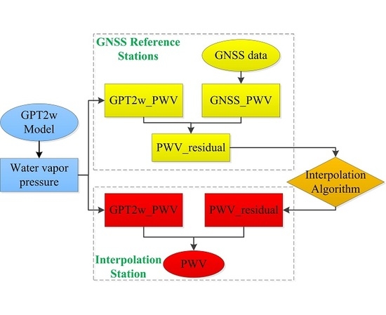
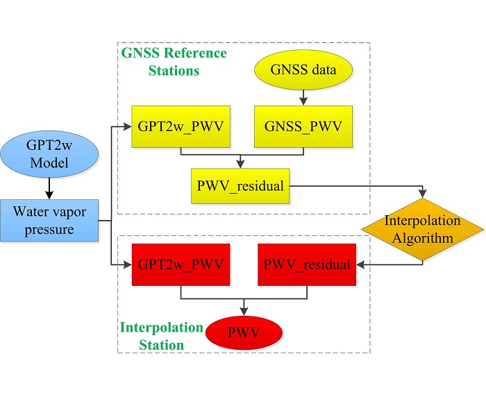
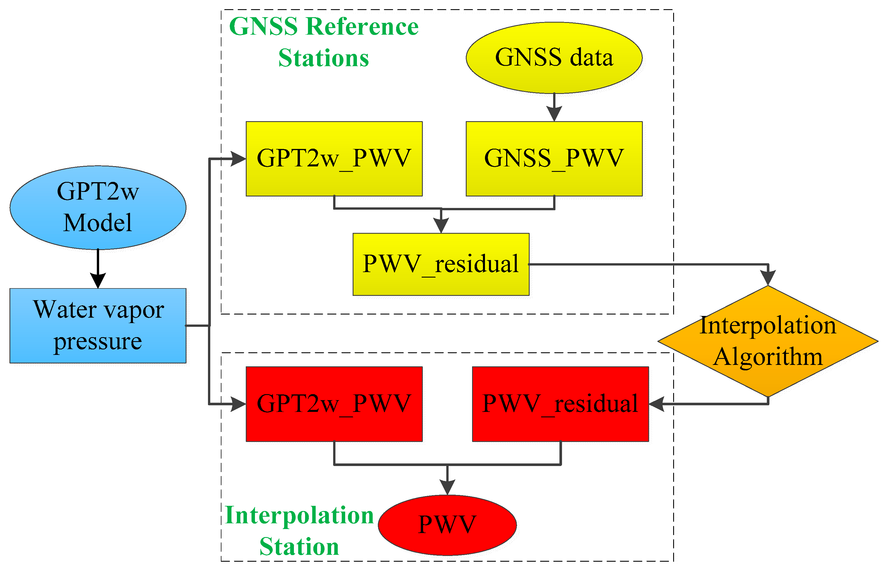
2.2. Interpolation Algorithm

It is known that different interpolation algorithms can work better for different variables, and geographical factors such as station densities, climate regimes, and seasonality may influence the choice of interpolation algorithm and the accuracy of the results. We therefore chose three interpolation algorithms, i.e., IDW, Kriging, and TPS, which are the most commonly used in PWV interpolation [7,18,32].
IDW, based on the SYMAP algorithm by Shepard [9], is a kind of deterministic algorithm for interpolation with a known scattered set of stations. It can relate the unknown value of PWV in a defined station to the values of PWV achieved from GNSS stations, on the basis of the distance between stations. It assumes that each measured station has a local influence that diminishes with distance, that is, the closer a station is to the station of estimate, the higher its influence.
Kriging, developed by Krige [33,34] and Matheron [35], and, as pointed out by Hofstra et al. [36], is a type of stochastic interpolation algorithm that belongs to the best linear unbiased estimation. In the algorithm, the PWV of interest at every unknown station is given by a linear combination of the PWV in GNSS reference stations, each weighted, and with the sum of weights equal to one. The weights are determined based on the variogram model, which is a spatial covariance function used to describe the variability of the observations. Webster and Oliver explain the concept of Kriging in more detail in [37].
TPS, theoretically described by Wahba [38] and further developed for meteorology by Hutchinson [39], is a deterministic spatial interpolation algorithm. Like Kriging, TPS is also based on spatial covariance function, and their differences lie in how the function is defined. The generalized cross-validation error is minimized to define the function in TPS. Basically, this algorithm is designed to minimize the total curvature of the measurements in order to pass data values. It is a linear combination of the basis function of either Gaussian or elliptical.
Combining the GPT2w model with the interpolation algorithms above-mentioned, the PWV of interest station can be obtained. Figure 1 is a flowchart of PWV interpolation with the GPT2w model.

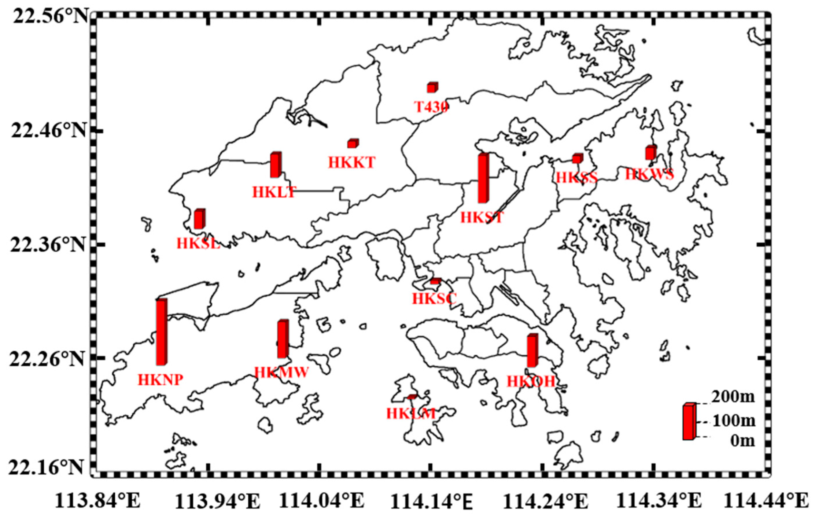
3. Experimental Description

This study utilized GNSS and the surface meteorological data of the Hong Kong Satellite Positioning Reference Station Network (SatRet) provided by the Hong Kong Geodetic Survey Services, which were freely downloaded via their website (www.geodetic.gov.hk). The GNSS data of 12 stations with a sampling rate of 30 s, and the surface meteorological data including temperature, pressure and relative humidity were downloaded. As shown in Figure 2, the area covered by those stations was 113.89°–114.34° for longitude and 22.21°–22.50° for latitude, respectively. The altitude ranges from 8.55 to 350.67 m, which is effective to detect the impact of elevation on PWV interpolation. Two periods with different weather conditions were selected in the experiment, one from 12 June to 18 June 2017 (DOY of 163 to 169, 2017) when Hong Kong suffered heavy rain with a maximum daily rainfall of 203.7 mm; the other was from 13 August to 19 August 2017 (DOY of 225 to 231, 2017) during rainless weather.
To achieve GNSS PWV, the GAMIT 10.61 software was adopted for the data processing based on the double-differenced model. In the processing, three international GNSS service (IGS) stations (SHAO, BJFS and LHAZ) were incorporated to reduce the strong correlation of tropospheric parameters caused by the short baselines between GNSS stations. The IGS precise ephemeris was used and a cutoff elevation angle of 10° was selected. The global mapping function (GMF) and the antenna phase center model based on the azimuth- and elevation-dependent data recommended by IGS was used. The IERS (International Earth Rotation and Reference System Service) Earth orientation parameters and the FES2004 model were applied during data processing. The LC_AUTCLN and BASELINE were selected as the processing strategies, representing the GNSS observations as ionosphere-free linear combinations and the fixed orbital parameters, respectively. After obtaining the ZHD using Equation (3), ZWD can be converted to PWV based on Equation (1), all of which require measured meteorological data.
In order to verify the validity of the interpolation algorithm proposed in this paper, different schemes were conducted in the experiment. For the first set, the IDW, Kriging, and TPS algorithm without the GPT2w model were used directly regardless of the elevation effect; the difference between the second set of schemes and the first set was the addition of the GPT2w model; for the third set, the three-dimensional (3D) Kriging and TPS algorithm that take into account the impact of elevation were utilized; and then the GPT2w model was added to the third set to form the fourth set. Thus, 10 PWV interpolation schemes were constructed in the experiment, i.e., IDW, Kriging, and TPS for the first set, IDW-GPT2w, Kriging-GPT2w, and TPS-GPT2w for the second set, 3DKriging and 3DTPS for the third set, and 3DKriging-GPT2w and 3DTPS-GPT2w for the fourth set. By using these interpolation schemes, the improvement of the elevation-dependent interpolation method was verified, and the effect of adding the GPT2w model under different circumstances was assessed.
In the experiment, two approaches for comparison were adopted. The first was the station cross-validation [40], where each station is excluded in turn and the PWV of the station are interpolated from the reference stations. Then, the observed and interpolated PWV at the excluded station are compared, enabling us to quantify the relative skill of different interpolation schemes at interpolating point values. The second approach was to interpolate the PWV on grid points, the locations of which are consistent with the European center for medium-range weather forecasts (ECMWF) data with a resolution of 0.125°*0.125°. The ECMWF can provide PWV on these grid points for a comparison of the interpolation across the entire region.
Several skill scores such as the compound relative error (CRE), mean absolute error (MAE), and root mean square error (RMSE) were utilized to study the performance of each interpolation scheme. Different skill scores highlight different features of the result [15]. MAE is an unambiguous, natural measure of average error, which is expressed in the same unit as the PWV itself. RMSE is used as a measure of deviation from the observed value and depends on the squared error means and has sensitivity to large outliers. CRE is a measure of similarity between the observed and interpolated values, namely, the ratio between the mean squared error and the variance of the observed values. The equations are presented below, where o is the observed, or reference series (PWV derived from GNSS data or ECMWF data), and y is the series to interpolate.
M A E = 1 n   i = 1 n | y i o i |
R M S E = 1 n   i = 1 n ( y k o k ) 2
C R E = i = 1 n ( y i o i ) 2 i = 1 n ( o k o ¯ ) 2

4. Result and Discussion

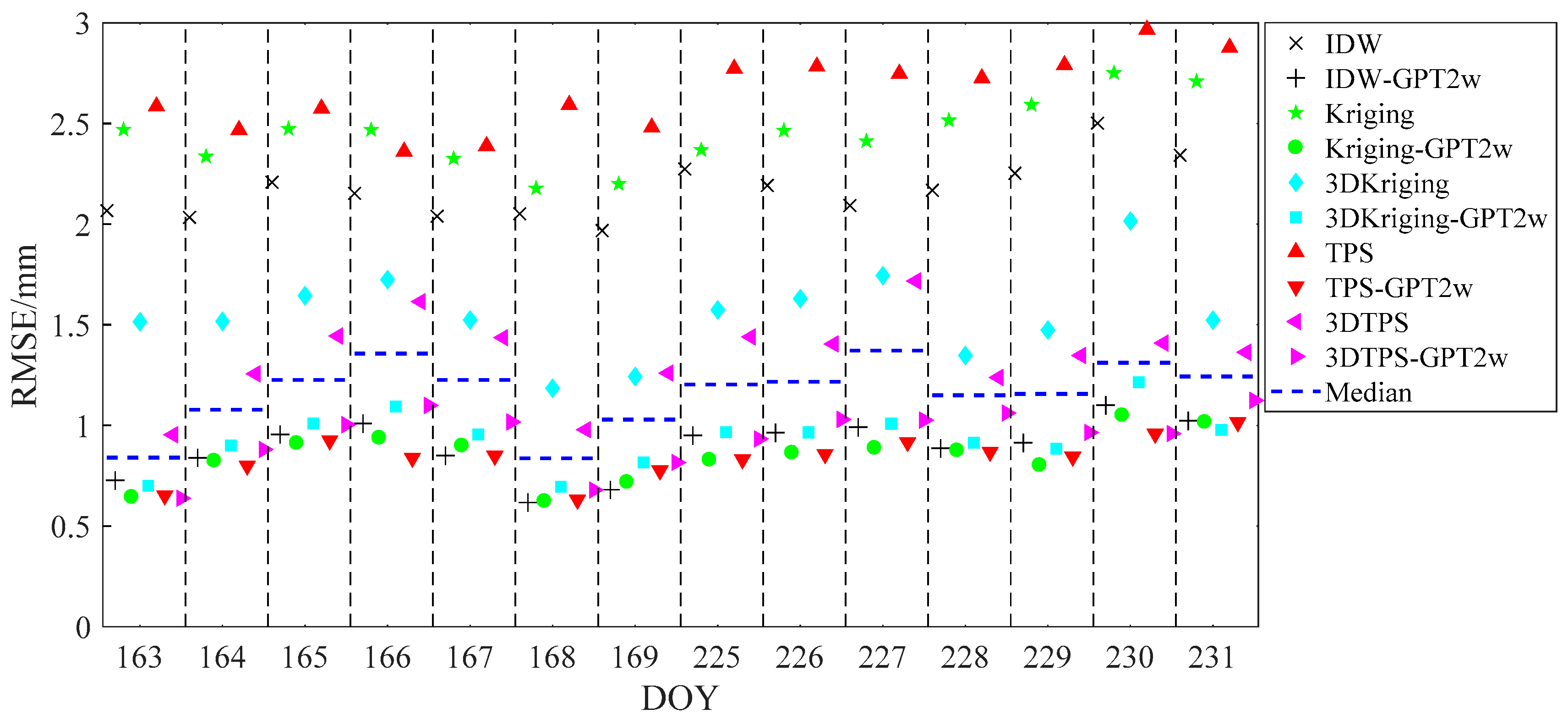
4.1. Station Cross-Validation

For the station cross-validation, each interpolation scheme was run 12 times for each period with 11 reference stations and one interpolation station. In Table 1, the average values of the skill scores in the 12 runs including RMSE, MAE, and CRE for each interpolation scheme with their corresponding rank (#) are shown. From the average ranks, it can be seen that the second set of schemes mentioned in Section 3 achieved the optimal results, followed by the fourth set, the third set, and the first set, which indicates that the addition of the GPT2w model, in any case, could result in a better interpolation result. Some other useful conclusions can be drawn, i.e., TPS and Kriging are extremely ineffective when the impact of terrain elevation is not taken into account, especially the TPS, instead the IDW should be used in this situation; once the terrain elevation is considered, 3DKriging and 3DTPS would be effective in improving the PWV interpolation results, especially the 3DTPS, once again indicating the importance of elevation information for PWV interpolation. It was noted that the interpolation results of the fourth set were slightly worse than those of the second set, that is, Kriging-GPT2w was better than 3DKriging-GPT2w and TPS-GPT2w was better than 3DTPS-GPT2w, respectively. This is mainly because the elevation information of the interpolation station was considered in the GPT2w model. Some inconsistencies and errors are likely to be introduced if the interpolation algorithm referred to the terrain elevation again.
From the comparison of the results between rainless and rainy weather conditions, it was found that the PWV interpolation results of each scheme on rainy days were slightly better than those on rainless days. To clarify this, the observed PWV, namely the PWV derived from GNSS data, in each GNSS station during the two periods were collected and counted. In Figure 3, the horizontal and vertical axes denote the GNSS stations and observed PWV values, respectively. Obviously, in the upper graph, the value of PWV on rainy days (blue ones) was larger than that of rainless days (red ones), but the fluctuation of PWV on rainy days was even smaller. Furthermore, the boxplots, which is a method for graphically depicting groups of numerical through their quartiles, are shown in the lower graph. From the spacings between the different parts of the box, the PWV data of rainy days in each station had a smaller degree of dispersion than that of rainless days. When comparing all the PWV data for different weather conditions, namely the black ones, it can be found that the PWV during the rainless period was relatively unstable and had a wider range of changes. This is why all interpolation schemes have a better performance on rainy days than on rainless days.
To further demonstrate the performance of different interpolation schemes, the RMSE of each day for station cross-validation is drawn in Figure 4, where the colors and symbols indicate the interpolation schemes. It is clear that the first set of schemes, i.e., IDW, Kriging, and TPS, performed the worst and had a larger RMSE, and the third set of schemes (3DKriging and 3DTPS) reduced the RMSE value due to the consideration of terrain elevation. With the addition of the GPT2w model, RMSE values were reduced again and the corresponding schemes achieved the best performance. The median value of all interpolation schemes on each day is also represented by the dotted blue line in each bin, which highlights the difference between the interpolation schemes. It separates the schemes by adding the GPT2w model from the schemes that are not added, showing the improvement of the GPT2w model for PWV interpolation. Additionally, as the figures of MAE and CRE are similar to the RMSE, they are not repeated here.
The map of the station RMSE (Figure 5) shows that the ten interpolation schemes performed quite nonuniformly all over the study area. The maps of the station MAE and CRE are not shown in this paper due to their similarities with RMSE. For each interpolation scheme, the station with the largest RMSE always appeared at HKNP, which had the highest elevation and was clearly outside the elevation range of other stations that can be seen from Figure 2. This demonstrates that the elevation has an important influence on the accuracy of PWV interpolation. It is particularly visible that the graphs on the right side of Figure 5, representing the PWV interpolation schemes with the addition of the GPT2w model, showed the improved RMSE of all stations compared to the graphs on the left without adding the GPT2w model.
Comparing (c) with (e), namely Kriging and 3DKriging, it was found that the interpolation scheme that only considered the elevation could also improve the PWV interpolation accuracy of most stations, but the improvements of some stations were not significant, especially station HKNP. When HKNP was regarded as the interpolation station, its elevation was not within the elevation range of the other 11 reference stations, and the difference was large. Thus, even if the 3DKriging scheme takes into account the influence of the elevation, the 11 reference stations cannot provide a sufficiently reliable reference on the elevation to the HKNP station and the improvement of the interpolation accuracy may not be much. This can also be proven by another phenomenon, that is, the accuracy improvement of the HKST station. As can be seen from Figure 2, HKST is the second highest station, and its elevation is very different from most other stations, so the Kriging interpolation scheme had poor accuracy. When 3DKriging was used, the elevation of HKST was included in the range of the reference station elevations, so there was a significant improvement in accuracy. It is conceivable that if there are other stations with elevations similar to that of HKST as the reference stations, that the improvement would be even greater. Similarly, if there is a station with an elevation higher than HKNP added as a reference station, the 3DKriging can perform better on station HKNP. For stations HKNP and HKST, the improvement of RMSE was 0.83/2.73 mm, from 5.98/4.83 mm for the Kriging scheme to 5.15/2.10 mm for 3DKriging. The above discussion indicates that the 3DKriging scheme relies heavily on the selection of the reference stations to improve the interpolation accuracy, and requires the elevation range of the reference stations to cover the elevation of the interpolation station as much as possible. In addition, the 3DTPS scheme also had the same problems. Thus, it can be concluded that the 3DKriging and 3DTPS scheme offer only slight improvements on PWV interpolation, when the range of the reference stations has insufficient coverage or the elevation of the interpolation station is special, like station HKNP. This is the biggest problem with traditional interpolation algorithms that take into account the impact of elevation.
As can be seen from the graphs on the right side of Figure 5, the above problem was well solved for the interpolation schemes that added the GPT2w model. For station HKNP, the improvement to RMSE was 4.40 mm from 5.98 mm for the Kriging scheme to 1.58 mm for the Kriging-GPT2w scheme, and was 2.89 mm from 4.34 mm from the TPS scheme to 1.45 mm for the TPS-GPT2w scheme. Additionally, it is clear that the addition of the GPT2w model not only improved the accuracy of the interpolation station with special elevation, but also had a better performance on all other stations when compared with the traditional schemes that only considered the effect of elevation (3DKriging and 3DTPS). For (d) and (f), that is, the Kriging-GPT2w and the 3DKriging-GPT2w schemes, their interpolation accuracy was similar, and the Kriging-GPT2w was slightly better than the 3DKriging-GPT2w at each station, of which the improvement was around 0.1 mm. This was also the case for the TPS-GPT2w and 3DTPS-GPT2w schemes. As mentioned in the previous section, multiple introductions of the elevation information in the interpolation can make the result worse. However, for the difference between each station, more research on the algorithm itself needs to be done in the future such as the assignment of the elevation weighting factors to explain the above phenomenon in more detail.

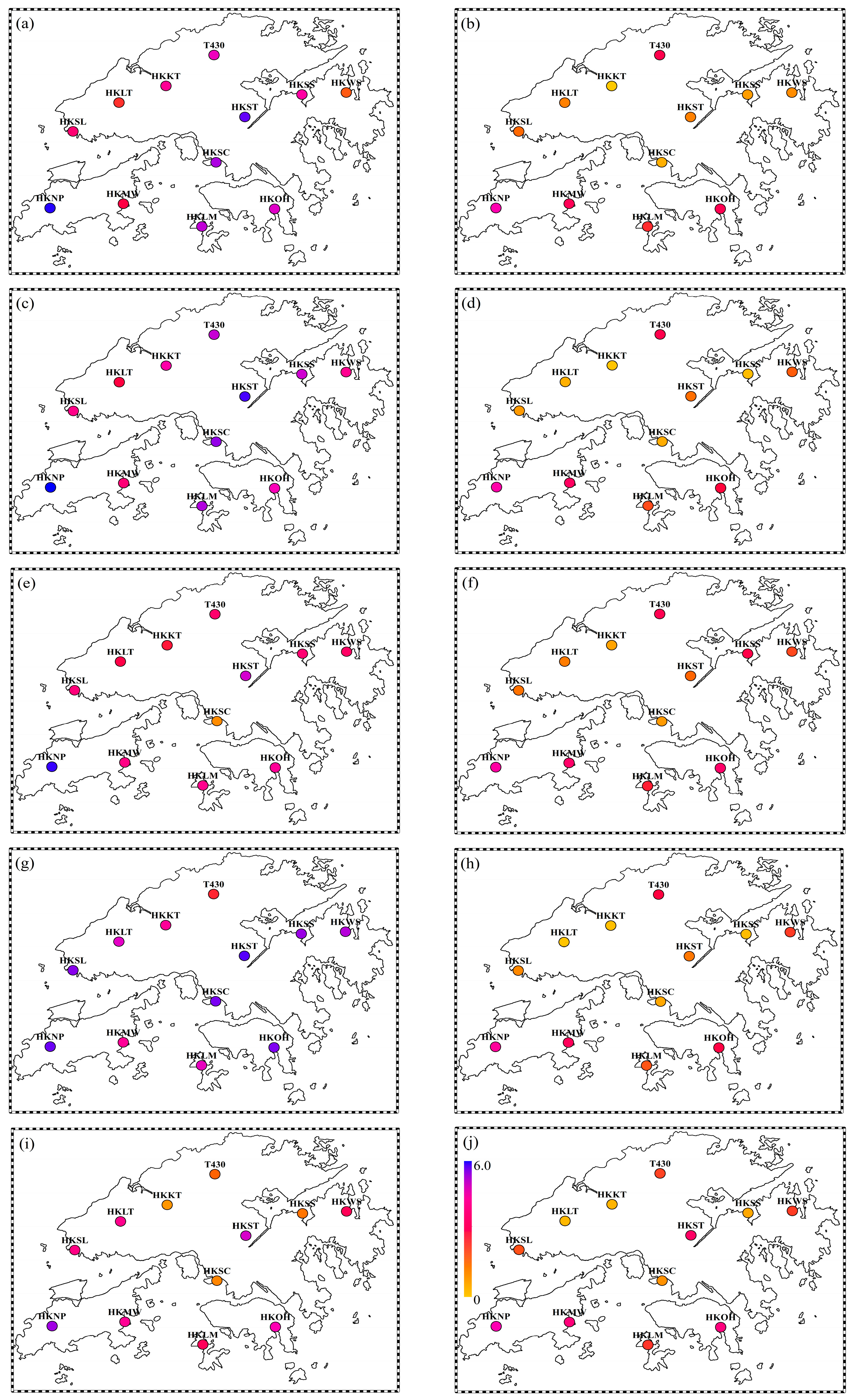
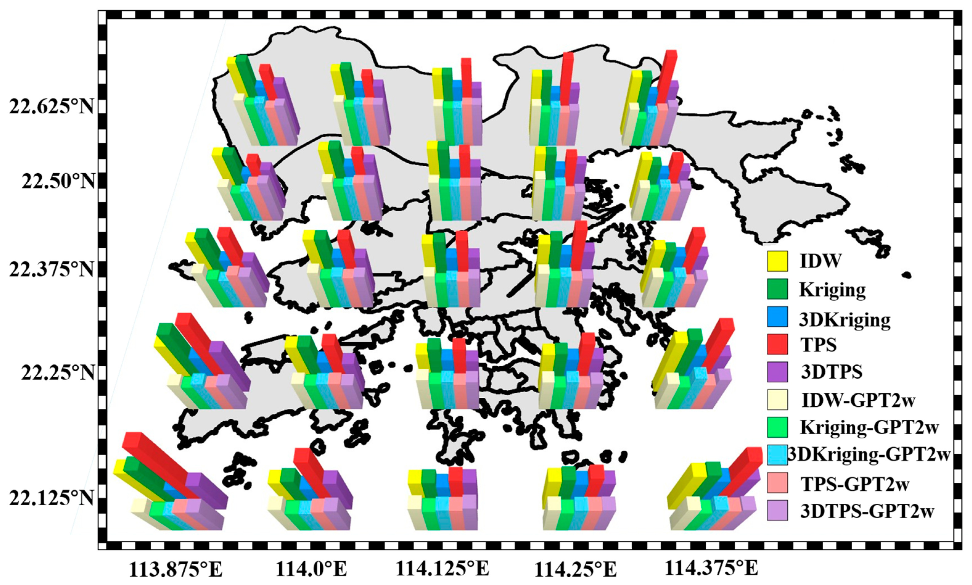
4.2. Grid Data Validation

As noted earlier, we used the ECMWF gridded data to evaluate the ability of each interpolation scheme in producing accurate grid estimates. In the research region, 25 grid points with the resolution of 0.125°*0.125° were selected, ranging from 113.875° to 114.375° for longitude and from 22.125° to 22.625° for latitude. The geopotential height of the grid points was included in the ECMWF data, and converted to the geometric height before interpolation [41]. As with the station cross-validation, we calculated the skill scores between the interpolated grid values and the ECMWF gridded data (as reference data). The summaries of the performance evaluation of different interpolation schemes are listed in Table 2. Overall, the skill scores were similar for grid data validation and station cross-validation. The third set of interpolation schemes that considered elevation effects (3DKriging and 3DTPS) was better than those of the first set without consideration (Kriging and TPS). All of the interpolation schemes that added the GPT2w model could improve the interpolation accuracy accordingly. However, there were some differences with the station cross-validation. For example, the Kriging-GPT2w scheme obtained the first rank instead of the TPS-GPT2w scheme, and the rank of the IDW-GPT2w scheme dropped. This demonstrates that the best performing interpolation scheme, after adding the GPT2w model, could be affected by the specific experimental conditions. This is similar to the situation without considering the GPT2w model in the previous study [42,43,44,45]. In addition, the skill scores of all schemes in the grid data validation were higher than in the station cross-validation, whether they were MAE, RMSE, or CRE. This is mainly due to the overall difference in the PWV obtained from the ECMWF gridded data and derived from the GNSS data.
To intuitively display the interpolation results in the grid points validation, the histogram of RMSE at 25 grid points for the 10 interpolation schemes is shown in Figure 6. The five pillars in the south of each grid point, representing the schemes that added the GPT2w model, are shorter than the corresponding five pillars to the north, which indicates that the addition of the GPT2w model can improve the interpolation accuracy at all grid points. Some other trends are the same as those in Table 2. Moreover, it was found that all of the interpolation schemes performed slightly worse at the grid points at the boundary of the study area, which is related to their being away from the reference stations.

5. Conclusions

In this paper, to analyze the improvement of PWV interpolation results after adding the GPT2w model, three types of interpolation algorithm, i.e., IDW, Kriging and TPS, were selected to construct 10 interpolation schemes. The station cross-validation and grid data validation were conducted in Hong Kong and the performance of different schemes was evaluated by several skill scores.
There exist differences in the PWV interpolation results of various weather conditions, which has little relationship with the interpolation scheme, and mainly depends on the stability of the PWV in the research region during the experimental period. This is the reason why the interpolation results of various schemes on rainless days are worse than on rainy days.
It was demonstrated that the addition of the GPT2w model can improve the PWV interpolation accuracy for each interpolation algorithm. However, it is best to add the model to the original interpolation algorithm, that is, the algorithm that ignores the impact of elevation, instead of the 3DKriging and 3DTPS. Since the initial PWV estimated by the GPT2w model is based on coordinate information of the interpolation point, the influence of elevation on the PWV was included. The introduction of the elevation factor again during the interpolation algorithm may bring additional errors, which is fully reflected in our experiment.
In some special cases such as station HKNP, whose elevation is far from the elevation range of reference stations, it was difficult for the reference stations to provide sufficient and reliable interpolation information in elevation direction, which is the restriction of the traditional interpolation algorithms. These deficiencies can be compensated by the GPT2w model, which estimates the initial PWV based on the elevation of the interpolation station. The PWV residual, a part of the PWV that is not related to the elevation, is then interpolated by the interpolation algorithms without considering the elevation range of the reference stations. It was proven in this paper that the addition of the GPT2w model can improve the PWV interpolation accuracy at any position.
Grid data validation was carried out in our experiment and its skill scores were slightly worse than those of the station cross-validation due to the overall difference in the ECMWF PWV and GNSS PWV. However, a good improvement in interpolation accuracy could be seen after adding the GPT2w model. This means that the schemes proposed in this paper can provide a more accurate value of PWV interpolation to the InSAR atmospheric calibration in the follow-up study. In addition, a more accurate conversion model for water vapor pressure and PWV should be studied in the future.

Author Contributions

Conceptualization, F.Y. and J.G.; Data curation, X.M.; Formal analysis, J.G.; Methodology, F.Y. and X.M.; Resources, J.S. and L.Z.; Validation, F.Y.; Writing—original draft, F.Y.; Writing—review & editing, J.G., X.M., J.S. and L.Z.

Funding

This research was funded by [National Natural Science Foundation of China] grant number [41474004], and [Natural Science Foundation of Guangxi Zhuang Autonomous Region] grant number [2018GXNSFBA050006].

Acknowledgments

The authors would like to thank the Lands Department of HKSAR for providing the GNSS data from the HONG KONG Satellite Positioning Reference Station Network (SatRef). Acknowledgements are also given to the editor in charge and anonymous reviewers for their valuable comments and suggestions to improve this manuscript. Our thanks also to the Chinese Scholarship Council (CSC) and the University of Nottingham for providing the opportunity for the first author to study at the University of Nottingham for one year.

Conflicts of Interest

The authors declare no conflict of interest.

References

  1. Bevis, M.; Businger, S.; Herring, T.A.; Rocken, C.; Anthes, R.A.; Ware, R.H. GPS meteorology: Remote sensing of atmospheric water vapor using the Global Positioning System. J. Geophys. Res. Atmos. 1992, 97, 15787–15801. [Google Scholar] [CrossRef]
  2. Rocken, C.; Ware, R.; Hove, T.V.; Solheim, F.; Alber, C.; Johnson, J.; Bevis, M.; Businger, S. Sensing atmospheric water vapor with the global positioning system. Geophys. Res. Lett. 1993, 20, 2631–2634. [Google Scholar] [CrossRef]
  3. Nilsson, T.; Gadinarsky, L.; Elgered, G. GPS tomography using phase observations. In Proceedings of the 2004 IEEE International Geoscience and Remote Sensing Symposium, Anchorage, AK, USA, 20–24 September 2004; pp. 2756–2759. [Google Scholar]
  4. Perler, D.; Geiger, A.; Hurter, F. 4D GPS water vapor tomography: New parameterized approaches. J. Geod. 2011, 85, 539–550. [Google Scholar] [CrossRef]
  5. Guo, J.; Yang, F.; Shi, J.; Xu, C. An optimal weighting method of Global Positioning System (GPS) troposphere tomography. IEEE J. Sel. Top. Appl. Earth Obs. Remote Sens. 2016, 9, 5880–5887. [Google Scholar] [CrossRef]
  6. Emardson, T.R.; Johansson, J.M. Spatial interpolation of the atmospheric water vapor content between sites in a ground-based GPS Network. Geophys. Res. Lett. 1998, 25, 3347–3350. [Google Scholar] [CrossRef]
  7. Suparta, W.; Rahman, R. Spatial interpolation of GPS PWV and meteorological variables over the west coast of Peninsular Malaysia during 2013 Klang Valley Flash Flood. Atmos. Res. 2016, 168, 205–219. [Google Scholar] [CrossRef]
  8. Sibson, R. A brief description of natural neighbour interpolation. In Interpreting Multivariate Data; Barnett, V., Ed.; John Wiley: New York, NY, USA, 1981; pp. 21–36. [Google Scholar]
  9. Shepard, D.S. Computer Mapping: The SYMAP interpolation algorithm. Spat. Stat. Models 1984, 40, 133–145. [Google Scholar]
  10. Hewitson, B.; Crane, R. Self-organizing maps: Applications to synoptic climatology. Clim. Res. 2002, 22, 13–26. [Google Scholar] [CrossRef]
  11. Jarlemark, P.; Emardson, T.R. Strategies for spatial and temporal extrapolation and interpolation of zenith wet delay. J. Geod. 1998, 72, 350–355. [Google Scholar] [CrossRef]
  12. Janssen, V.; Ge, L.; Rizos, C. Tropospheric correction to SAR interferometry from GPS observations. GPS Solut. 2004, 8, 140–151. [Google Scholar] [CrossRef]
  13. Yin, H.; Dang, Y.; Xue, S.; Nie, J. An interpolation method for zenith tropospheric delay based on higher taylor series expansion. J. Geod. Geodyn. 2013, 33, 155–159. (In Chinese) [Google Scholar]
  14. Yang, S.; Zhang, Q.; Zhang, S.; Zhao, C. Research on GPS water vapor interpolation by improved Kriging algorithm. Remote Sens. Land Resour. 2013, 25, 39–43. (In Chinese) [Google Scholar]
  15. Vicente-Serrano, S.; Saz-Sanchez, M.; Cuadrat, J. Comparative analysis of interpolation methods in the middle Ebro Valley (Spain): Application to annual precipitation and temperature. Clim. Res. 2003, 24, 161–180. [Google Scholar] [CrossRef]
  16. Li, Z.; Fielding, E.; Cross, P.; Muller, J. Interferometric synthetic aperture radar atmospheric correction: GPS topography dependent turbulence model. J. Geophys. Res. Solid Earth 2006, 111, B02404. [Google Scholar] [CrossRef]
  17. Li, Z.; Ding, X.; Huang, C.; Wadge, G.; Zheng, D. Modeling of atmospheric effects on InSAR measurements by incorporating terrain elevation information. J. Atoms. Sol. Terres. Phys. 2006, 68, 1189–1194. [Google Scholar] [CrossRef]
  18. Xu, W.; Li, Z.; Ding, X.; Zhu, J. Interpolating atmospheric water vapor delay by incorporating terrain elevation information. J. Geod. 2011, 85, 555–564. [Google Scholar] [CrossRef]
  19. Onn, F.; Zebker, H.A. Correction for interferometric synthetic aperture radar atmospheric phase artifacts using time series of zenith wet delay observations from a GPS network. J. Geophys. Res Solid Earth 2006, 111, B09102. [Google Scholar] [CrossRef]
  20. Bohm, J.; Moller, G.; Schindelegger, M.; Pain, G.; Weber, R. Development of an improved empirical model for slant delays in the troposphere. GPS Solut. 2015, 19, 433–441. [Google Scholar] [CrossRef]
  21. Bevis, M. GPS meteorology: Mapping zenith wet delays onto precipitable water. J. Appl. Meteorol. 1994, 33, 379–386. [Google Scholar] [CrossRef]
  22. Yang, F.; Guo, J.; Shi, J.; Zhou, L.; Xu, Y.; Chen, M. A Method to Improve the Distribution of Observations in GNSS Water Vapor Tomography. Sensors 2018, 18, 2526. [Google Scholar] [CrossRef]
  23. Liu, Y.; Chen, Y.; Liu, J. Determination of weighted mean tropospheric temperature using ground meteorological measurement. Geo-Spat. Inf. Sci. 2001, 4, 14–18. [Google Scholar]
  24. Yao, Y.; Zhu, S.; Yue, S. A globally applicable, season-specific model for estimating the weighted mean temperature of the atmosphere. J. Geod. 2012, 86, 1125–1135. [Google Scholar] [CrossRef]
  25. Saastamoinen, J. Atmospheric correction for the troposphere and stratosphere in radio ranging satellites. Use Artif. Satell. Geod. 1972, 15, 247–251. [Google Scholar]
  26. Karalis, J.D. Precipitable Water and Its Relationship to Surface Dew Point and Vapor Pressure in Athens. J. Appl. Meteorol. 1974, 13, 760–766. [Google Scholar] [CrossRef]
  27. Cole, R.J. Direct solar radiation data as input into mathematical models describing the thermal performance of buildings—II. Development of relationships. Build. Sci. 1976, 11, 181–186. [Google Scholar] [CrossRef]
  28. Li, C.; Wei, H.; Liu, H.; Zhou, J. Statistics of Correlation of Integrated Water Vapor and Surface Vapor Pressure. Geomat. Inf. Sci. Wuhan Univ. 2008, 33, 1170–1173. [Google Scholar]
  29. Reber, E.; Swope, J. On the correlation of the total precipitable water in a vertical column and absolute humidity at the surface. J. Appl. Meteorol. 1972, 11, 1322–1325. [Google Scholar] [CrossRef]
  30. Huang, Y.; Jiang, D.; Zhuang, D. An operational approach for estimating surface vapor pressure with satellite-derived parameter. Afr. J. Agric. Res. 2010, 5, 2817–2824. [Google Scholar]
  31. Zhang, X. A relationship between precipitable water vapor and surface vapor pressure. Meteorol. Mon. 2004, 30, 9–11. (In Chinese) [Google Scholar]
  32. Camera, C.; Bruggeman, A.; Hadjinicolaou, P.; Pashiardis, S.; Lange, M. Evaluation of interpolation techniques for the creation of gridded daily precipitation (1 × 1 km2); Cyprus, 1980–2010. J. Geophys. Res. Atmos. 2014, 119, 693–712. [Google Scholar] [CrossRef]
  33. Krige, D. A statistical approach to some basic mine valuation problems on the Witwatersrand. J. Chem. Metall. Min. Soc. S. Afr. 1951, 52, 119–139. [Google Scholar]
  34. Krige, D. Two-dimensional weighted moving average trend surfaces for ore evaluation. J. S. Afr. Inst. Min. Metall. 1966, 66, 13–38. [Google Scholar]
  35. Matheron, G. Principles of geostatistics. Econ. Geol. 1963, 58, 1246–1266. [Google Scholar] [CrossRef]
  36. Hofstra, N.; Haylock, M.; New, M.; Jones, P.; Frei, C. Comparison of six methods for the interpolation of daily European climate data. J. Geophys. Res. 2008, 113, D21110. [Google Scholar] [CrossRef]
  37. Webster, R.; Oliver, M. Geostatistics for Environmental Scientists. Statistics in Practice; John Wiley and Sons: Chichester, UK, 2001. [Google Scholar]
  38. Wahba, G. Spline models for observational data. In CBMS-NSF Regional Conference Series in Applied Mathematics; Society for Industrial and Applied Mathematics: Philadelphia, PA, USA, 1990; Book 59. [Google Scholar]
  39. Hutchinson, M. Interpolation of rainfall data with thin plate smoothing splines-Part I: Two-dimensional smoothing of data with short range correlation. J. Geogr. Inf. Decis. Anal. 1998, 2, 152–167. [Google Scholar]
  40. Willmott, C.; Matsuura, K. Smart interpolation of annually averaged air temperature in the United States. J. Appl. Meteorol. 1995, 34, 2577–2586. [Google Scholar] [CrossRef]
  41. Wang, X.; Zhang, K.; Wu, S.; Fan, S.; Cheng, Y. Water vapor-weighted mean temperature and its impact on the determination of precipitable water vapor and its linear trend. J. Geophys. Res.-Atmos. 2016, 121, 833–852. [Google Scholar] [CrossRef]
  42. Willmott, C.; Robeson, S.; Feddema, J. Estimating continental and terrestrial precipitation averages from rain-gauge networks. Int. J. Climatol. 1994, 14, 403–414. [Google Scholar] [CrossRef]
  43. Price, D.; McKenney, D.; Nalder, I.; Hutchinson, M.; Kesteven, J. A comparison of two statistical methods for spatial interpolation of Canadian monthly mean climate data. Agric. For. Meteorol. 2000, 10, 81–94. [Google Scholar] [CrossRef]
  44. Daly, C.; Gibson, W.; Taylor, G.; Johnson, G.; Pasteris, P. A knowledge-based approach to the statistical mapping of climate. Clim. Res. 2002, 22, 99–113. [Google Scholar] [CrossRef]
  45. Hewitson, B.; Crane, R. Gridded area-averaged daily precipitation via conditional interpolation. J. Clim. 2005, 18, 41–57. [Google Scholar] [CrossRef]
Figure 1. Flowchart of PWV interpolation with the GPT2w model.
Remotesensing 11 01127 g001
Figure 2. Geographic distribution of GNSS stations and their elevations.
Remotesensing 11 01127 g002
Figure 3. Scatter (upper) and boxplot (lower) of the observed PWV at each station during the period of rainless and rainy days. Blue for the rainy condition and red for the rainless condition.
Remotesensing 11 01127 g003
Figure 4. RMSE of different interpolation schemes on each day for station cross-validation.
Remotesensing 11 01127 g004
Figure 5. Map showing RMSE at the 12 stations for the 10 interpolation schemes in rainy weather condition. (a) IDW, (b) IDW-GPT2w, (c) Kriging, (d) Kriging-GPT2w, (e) 3DKriging, (f) 3DKriging-GPT2w, (g) TPS, (h) TPS-GPT2w, (i) 3DTPS, (j) 3DTPS-GPT2w.
Remotesensing 11 01127 g005
Figure 6. Histogram of RMSE at 25 grid points for the 10 interpolation schemes.
Remotesensing 11 01127 g006
Table 1. Summary of the performance evaluation of different interpolation schemes for station cross-validation (left for rainless and right for rainy weather condition).
Rainless WeatherRainy Weather
MethodMAE#RMSE#CRE#MAE#RMSE#CRE#
[mm] [mm] [-] [mm] [mm] [-]
IDW2.11882.28580.24481.96182.01080.5888
IDW-GPT2w0.78031.00430.03730.66530.83830.0733
Kriging2.37392.57090.29292.20492.37590.72310
Kriging-GPT2w0.72810.92820.03220.65220.82020.0702
3DKriging1.37771.67070.13271.27271.51770.3437
3DKriging-GPT2w0.79341.02440.03840.72350.90940.0824
TPS2.701102.818100.312102.412102.512100.6859
TPS-GPT2w0.73120.91410.03210.64210.80810.0671
3DTPS1.10561.44960.08161.00561.30960.1936
3DTPS-GPT2w0.81251.03650.03950.71940.91150.0875
Table 2. Summary of the performance evaluation of different interpolation schemes for grid points comparison with the ECMWF data.
MethodMAE#RMSE#CRE#
[mm] [mm] [-]
IDW2.45982.96580.4628
IDW-GPT2w1.64042.06450.1935
Kriging2.53793.02290.4729
Kriging-GPT2w1.47011.79110.1411
3DKriging1.82062.19260.2176
3DKriging-GPT2w1.58721.89520.1602
TPS2.873103.310100.69310
TPS-GPT2w1.62031.92930.1663
3DTPS1.97872.37370.2487
3DTPS-GPT2w1.69952.00740.1814

