Hybrid Grasshopper Optimization Algorithm and Differential Evolution for Multilevel Satellite Image Segmentation

Abstract

An efficient satellite image segmentation method based on a hybrid grasshopper optimization algorithm (GOA) and minimum cross entropy (MCE) is proposed in this paper. The proposal is known as GOA–jDE, and it merges GOA with self-adaptive differential evolution (jDE) to improve the search efficiency, preserving the population diversity especially in the later iterations. A series of experiments is conducted on various satellite images for evaluating the performance of the algorithm. Both low and high levels of the segmentation are taken into account, increasing the dimensionality of the problem. The proposed approach is compared with the standard color image thresholding methods, as well as the advanced satellite image thresholding techniques based on different criteria. Friedman test and Wilcoxon’s rank sum test are performed to assess the significant difference between the algorithms. The superiority of the proposed method is illustrated from different aspects, such as average fitness function value, peak signal to noise ratio (PSNR), structural similarity index (SSIM), feature similarity index (FSIM), standard deviation (STD), convergence performance, and computation time. Furthermore, natural images from the Berkeley segmentation dataset are also used to validate the strong robustness of the proposed method.

1. Introduction

Image segmentation is one of the most important techniques in image processing, which partitions a given image into several unique and disjoint classes according to color, texture, edge, and other parameters [1,2,3,4,5]. In the last few decades, many segmentation methods have been proposed by researchers, such as clustering, edge detection, region growing, and thresholding [6,7,8]. Among the available methods, thresholding is extensively used due its simplicity and efficiency [9]. In fact, the thresholding method can be divided into two categories: bi-level thresholding and multilevel thresholding. Bi-level thresholding is suitable for simple segmentation tasks, and splits the image into two classes, namely, foreground and background [10]. However, if the given image is informative and contains multiple objects, then classical bi-level thresholding is insufficient. The bi-level thresholding is, therefore, extended into multilevel thresholding to enhance applicability.

Several techniques have been introduced into this domain to determine the segmentation thresholds. Minimum cross entropy (MCE) is one of the most popular techniques and has attracted widespread attention in recent years [11]. The optimal thresholds were selected by minimizing the cross entropy between the original classes and the segmented classes. In 2015, Sarkar et al. introduced an MCE-based method for color image segmentation [12]. Three hundred distinct images from the Berkeley segmentation dataset were used to comprehensively evaluate the performance of the proposed method. From the results, it was found that the proposed thresholding method is superior over not only the meta-heuristic-based methods, but also other prominent algorithms. Pare et al. used an MCE-based approach to segment various color images with low resolution and poor illumination [13]. Both natural images and satellite images were selected for testing. Experimental results reveal that the proposed method can determine the thresholds more efficiently and accurately compared to other methods. In 2017, Oliva et al. proposed thresholding using MCE for magnetic resonance (MR) image segmentation [14]. The experimental results indicate that the obtained well-delimited regions were easier to distinguish than when other techniques [14]. These phenomena convincingly demonstrate the remarkable performance of the MCE method in the field of image segmentation.

However, there are still some drawbacks that limit the MCE method from wide application. For example, the computational complexity increases exponentially as the number of thresholds increases, and the exhaustive search that is used makes the algorithm inefficient. To overcome these drawbacks, many meta-heuristic algorithms and their modified versions have been adopted and combined with thresholding techniques, such as particle swarm optimization (PSO) [15], differential evolution (DE) [16], bat algorithm (BA) [17], dragonfly algorithm (DA) [18], and grey wolf optimizer (GWO) [19]. Suresh and Lal introduced a chaotic Darwinian particle swarm optimization (CDPSO)-based satellite image segmentation method [20]. Ten chaotic maps were used for testing, and the best one was chosen. MCE and Tsallis entropy criteria were used as objective functions. Mlakar et al. presented a hybrid differential evolution (hjDE)-based method for finding the optimal segmentation thresholds [21]. The reset strategy of cuckoo search (CS) was added into the hybrid model with the purposed of avoiding local optimization. In 2018, Satapathy et al. employed and validated a multilevel image thresholding technique based on chaotic bat algorithm (CBA) [22]. The chaotic Ikeda map was combined with the traditional BA to maintain population diversity and enhance search efficiency. Several standard test images, with different sizes, were used to evaluate the performance of the proposed method. In 2018, Díaz-Cortés et al. applied a DA-based thresholding approach to breast thermogram analysis [23]. The introduction of DA greatly reduced the computational complexity of the traditional thresholding method. Furthermore, the promising experimental results indicate that the proposed algorithm can provide reliable technical support for clinical decisions and has a certain application value. Khairuzzaman and Chaudhury proposed a multilevel thresholding approach based on GWO for gray image segmentation [24]. Two other meta-heuristic algorithm-based thresholding methods were utilized for comparison. Relevant results suggest that the GWO-based method can provide solutions of higher accuracy and stability. Additionally, some other algorithms were also applied to the field of multilevel image thresholding, including whale optimization algorithm (WOA) [25], Lévy flight firefly algorithm (LFA) [26], multiverse optimizer (MVO) [27], social spider optimization (SSO) [28], teaching–learning-based optimization (TLBO) [29], krill herd optimization (KHO) [30], adaptive wind driven optimization (AWDO) [31], modified firefly algorithm (MFA) [32]. These examples of successful applications have motivated us to introduce some novel and efficient meta-heuristic algorithms into this domain, and then obtain a high-performance method for multilevel satellite image thresholding.

On the other hand, the grasshopper optimization algorithm (GOA) is a recently proposed swarm intelligence (SI) technique that mimics the swarm behavior of grasshoppers in nature. Since being presented by Saremi et al. in 2017 [33], it has been widely used and shown a remarkable performance in many fields, such as financial stress prediction [34], feature selection [35], analysis of vibration signals from rotating machinery [36], optimal reconfiguration of partially shaded photovoltaic (PV) array [37], and more. In fact, the optimization ability of the GOA algorithm still needs to be effectively strengthened to better cope with different engineering problems. In [34], three strategies, namely Gaussian mutation, Lévy flight, and opposition-based learning (OBL), were adopted to achieve a more suitable balance between exploration and exploitation. In [38], the OBL strategy was introduced into the initialization and update stages of the optimization process, which can enhance the search efficiency and avoid local optimum to some extent. In [39], a natural selection strategy and democratic decision-making mechanism were used to avoid local best trap. In addition, the dynamic feedback mechanism based on the 1/5 principle was also introduced to adjust the parameter $c$ for better balancing global and local search [39]. The above phenomena motivate us to combine GOA with an efficient strategy to overcome the drawbacks, such as slow convergence speed, unbalanced exploration–exploitation, and local optimization.

Another interesting technique for optimization is differential evolution (DE) [16]. DE is a simple but powerful algorithm, which has been combined with other algorithms to enhance search efficiency and maintain population diversity. In 2017, Jadon et al. proposed a hybridization of artificial bee colony (ABC) and DE algorithms to develop a new meta-heuristic algorithm with better convergence speed and a better balance between exploration and exploitation abilities [40]. Dash et al. introduced a hybrid meta-heuristic technique known as hybrid firefly differential evolution (HFDE) [41]. The firefly movement was used as an additional search of DE to avoid local optimization and improve convergence performance. In 2018, Xiong et al. presented a hybrid WOA with DE, called DE/WOA, for extracting the accurate parameters of photovoltaic (PV) models [42]. DE also served as an additional search technique, and the crossover probability $\left(CR\right)$ was the criterion for using DE. To sum up, these promising results indicate the remarkable performance of DE in hybrid meta-heuristic algorithms. In fact, some of the available hybrid models still have drawbacks, for instance, a two-layer position update mechanism is often adopted, that is, after the first strategy completes the position update, the second one will be utilized to continue to update the position that has been updated once [43]. This type of approach does have certain advantages, especially the introduction of greedy selection strategy, which can prevent population stagnation and degradation caused by additional searching. However, the computational complexity of these methods is high, which is determined by the hybrid model used. In this paper, an alternative hybrid algorithm of GOA and jDE is proposed to overcome the above shortcoming.

Satellite images are one of the important sources of information which have been widely used in the field of geographic information systems, astronomy, and earth science [44]. Generally speaking, it is difficult to locate objects and boundaries in satellite images with poor illumination and complex backgrounds. Therefore, developing a high-performance color satellite image segmentation method is of significance and can provide reliable theoretical support for engineering practices. In this paper, a novel hybrid GOA with jDE is introduced for multilevel satellite image segmentation. The MCE technique is used to select the segmentation thresholds. In order to evaluate the algorithm performance objectively, a series of experiments are conducted on various satellite images. Both low and high levels of the thresholds are considered. The proposed method is compared with the standard color image thresholding methods as well as the advanced satellite image thresholding techniques based on different criteria. Comprehensive statistical analyses, including Friedman test and Wilcoxon’s rank sum test, are performed to assess the significant difference between the algorithms. The superiority of the proposed hybrid algorithm is illustrated from different aspects, such as average fitness function value, peak signal to noise ratio (PSNR), structural similarity index (SSIM), feature similarity index (FSIM), standard deviation (STD), convergence performance, and computation time. Besides, natural images from the Berkeley segmentation dataset are also used to validate the strong robustness of the proposed method.

The main contributions of this study have three aspects:

• Propose an efficient satellite image segmentation method.
• Apply the hybrid algorithm of GOA and DE to the multilevel thresholding domain.
• Introduce an alternative hybrid model for a meta-heuristic algorithm.

The structure of this paper is presented as follows: Section 2 briefly reviews the GOA. The definition of MCE thresholding technique is presented in Section 3. The proposed GOA–jDE-based multilevel satellite image thresholding method is illustrated in Section 4. In Section 5, a series of experiments are conducted, along with a detailed relevant discussion. Finally, Section 6 summarizes the conclusions of this paper and future work directions.

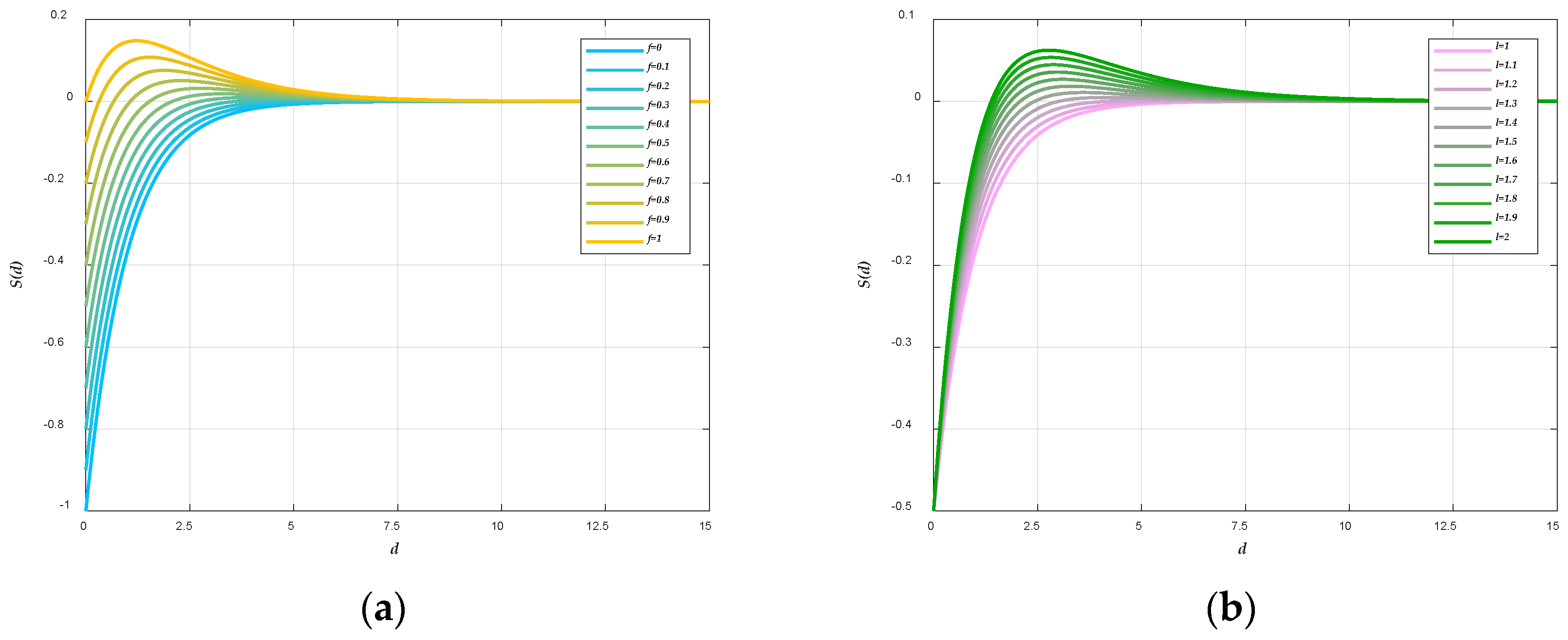
2. Grasshopper Optimization Algorithm

The grasshopper optimization algorithm is inspired by the swarming behavior of grasshoppers in nature. It was first proposed by Saremi et al. to determine the optimal shape of architectural structures [33]. There are three main factors that influence the movement of the grasshopper individual: social interaction, gravity force, and wind advection [34,45]. The mathematical model of their swarm behavior is given as follows:

$$X_i=S_i+G_i+A_i,$$

(1)

where $X_i$ is the position of the ith grasshopper. $S_i$, $G_i$, and $A_i$ indicate the social interaction, gravity force, and wind advection on the ith grasshopper, respectively.

However, Equation (1) cannot be directly utilized to solve optimization problems. The authors presented an improved version that was defined as

$$X_i^d=c\left({{\displaystyle \sum }}_{j=1,j\ne i}^{N}c\frac{u{b}_d-l{b}_d}{2}s\left(\left|x_j^d-x_i^d\right|\right)\frac{x_j-x_i}{d_{ij}}\right)+\widehat{T_d},$$

(2)

where $u{b}_d$ and $l{b}_d$ represent the upper bound and lower bound in the dth dimension, respectively. $\widehat{T_d}$ indicates the value of the dth dimension in the best solution obtained so far. $d_{ij}=\left|x_j-x_i\right|$ shows the distance between the ith grasshopper and jth grasshopper. $s$ is a designed function that can be calculated by $s\left(r\right)=f{e}^{-r/l}-e^{-r}$. $f$ and $l$ are two constants. In order to investigate the influence of $f$ and $l$ on $s$ function, two different cases were considered. The relevant results are shown in Figure 1.

$c$ is a significant parameter of GOA that can balance the exploration and exploitation of optimization. It decreases with the number of iterations and can be computed by

$$c=c_{max}-t\frac{c_{max}-c_{min}}{t_{max}},$$

(3)

where $c_{max}$ and $c_{min}$ are the maximum and minimum values, respectively. $t$ is the current iteration and $t_{max}$ indicates the maximum number of iterations.

Pseudocode of traditional GOA for global optimization is given in Algorithm 1.

Algorithm 1 Pseudocode of grasshopper optimization algorithm for optimization problem

1. Begin 2.   Initialize a randomly distributed population in the search space; 3.   Initialize the best search agent $\widehat{T_d}$; 4.   while $t<t_{\max }$ 5.     Evaluate $c$ using Equation (3); 6.     for $i=1:n$ 7.       Calculate the objective value of each grasshopper $f_i$; 8.       Update the best search agent $\widehat{T_d}$; 9.       Normalize the distance between grasshoppers in [1,4]; 10.      Update the position of grasshopper $x_i$ using Equation (2); 11.      Correct the position of the current grasshopper if it is beyond the border; 12.     end for 13.   end while 14.   return $\widehat{T_d}$, which represents the optimal position of optimization; 15. End

3. Multilevel Thresholding

Minimum cross entropy (MCE) technique determines the optimal thresholds based on minimizing the cross entropy between the original image and the segmented image, which shows remarkable performance in previous works by researchers [11,12,13,14]. It is worth mentioning that the segmentation operation of color images is more complex than that of grayscale images, as each color component (red, green, and blue) should be segmented. The objective function of the above thresholding technique is presented as follows:

$$f_{MCE}={\displaystyle \sum }_{i=0}^n-m_i^1\ln \left(\frac{m_i^1}{m_i^0}\right),$$

(4)

where $m_i^0={\sum }_{j=T_i}^{T_{i+1}-1}{p}_j$, $m_i^1={\sum }_{j=T_i}^{T_{i+1}-1}j{p}_j$, $p_j=h\left(j\right)/N$. $p_j$ is the proportion of pixels in each gray level to the total. $\left\{T_1,T_2,\dots ,T_n\right\}$ represents the combination of thresholds. $h\left(j\right)$ represents the frequency, and $N$ is the number of all pixels. Besides, for multilevel image thresholding, $T_0=0$ and $T_{n+1}=L$. $L$ is the number of gray levels in the given image.

Additionally, the computational complexity of thresholding technique above will result in exponential growth as the number of thresholds increase. In this case, the basic MCE multilevel thresholding method is not very effective. Thus, the GOA–jDE-based method using MCE is proposed with the purpose of reducing computational complexity and improving segmentation precision. In other words, the GOA–jDE algorithm is used to optimize the objective function given in Equation (4).

4. Proposed Methodology

In this section, a hybrid GOA algorithm with DE is introduced in detail. Firstly, the DE algorithm and its variant, jDE, are reviewed. Secondly, the hybrid model is discussed. Then, the proposed algorithm, namely GOA–jDE, is applied to multilevel satellite image segmentation domain, and the relevant flowchart is also presented. Finally, the computational complexity comparison between GOA and GOA–jDE is made.

4.1. Differential Evolution

Differential evolution (DE) is a simple and powerful evolutionary algorithm proposed by Storn and Price in 1997, which has attracted extensive attention over the past few decades [46,47]. There are three main operators in the DE algorithm, namely “mutation”, “crossover”, and ”selection” [48]. Scaling factor $SF$ and crossover probability $CR$ are two significant parameters which affect the exploration and exploitation phases of optimization.

4.1.1. Mutation

The mutation operation of DE algorithm can be calculated as

$$m_i^{t+1}=x_{r1}^t+SF\times \left(x_{r2}^t-x_{r3}^t\right),$$

(5)

where $m_i^{t+1}$ is the mutant individual in the $\left(t+1\right)\mathrm{th}$ iteration. $x_{r1}^t$, $x_{r2}^t$, and $x_{r3}^t$ indicate three different individuals in the population. More specifically, $r_1$, $r_2$, and $r_3$ are not equal. The scaling factor denoted by $SF$ is a constant here.

4.1.2. Crossover

After the process of mutation, the trial individual $c_i^{t+1}$ is chosen from the current individual $x_i^t$ or the mutant individual $m_i^{t+1}$ with the purpose of improving the population diversity. The crossover operation of DE algorithm is mathematically defined as follows:

$$c_i^{t+1}=\{\begin{array}{ll}{m}_i^{t+1}& if rand\le CR\\ x_i^t& if rand>CR\end{array},$$

(6)

where $rand$ is a uniformly distributed random number in the interval $\left[0,1\right]$. $CR$ is a constant that indicates the crossover probability.

4.1.3. Selection

During the process of selection, a comparison between the trial individual $c_i^{t+1}$ and the current individual $x_i^t$ is made to obtain an individual of $\left(t+1\right)\mathrm{th}$ generation. For a minimization problem, the selection operation is defined as

$$x_i^{t+1}=\{\begin{array}{cc}{c}_i^{t+1}\hfill & if f\left(c_i^{t+1}\right)<f\left(x_i^t\right)\\ x_i^t\hfill & otherwise\end{array},$$

(7)

where $f$ indicates the objective function of the given optimization problem.

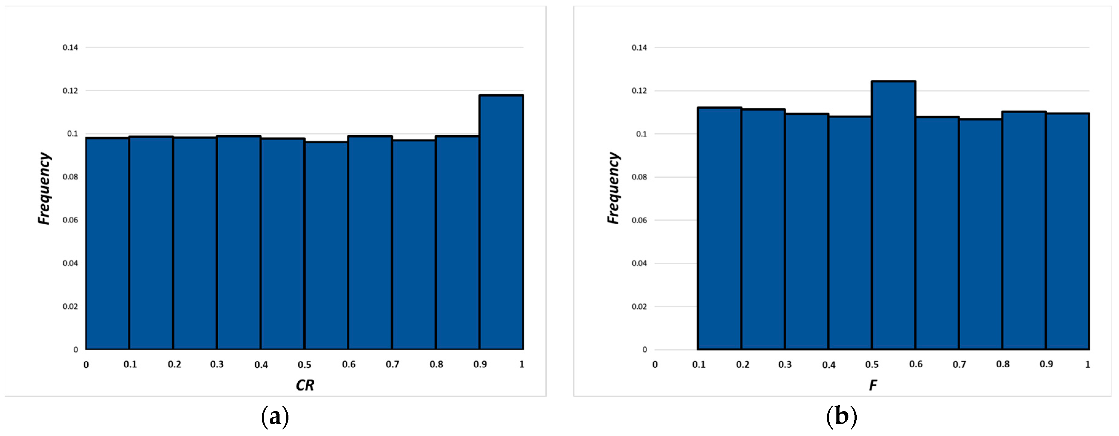
4.2. Self-Adapting Differential Evolution (jDE)

As discussed above, scaling factor $SF$ and crossover probability $CR$ are two significant parameters in the DE algorithm, the value of which can affect the optimization capability. In the standard DE, these two control parameters are constant throughout the entire evolutionary process. However, the fixed value cannot adapt well to various problems, especially complex high-dimensional problems. Therefore, Brest et al. [49] introduced a modified version of DE that can set the control parameters adaptively. In the modified DE, known as jDE, the control parameters $SF$ and $CR$ can be expressed as follows:

$$S{F}_i^{t+1}=\{\begin{array}{cc}S{F}_l+ran{d}_1\times S{F}_u\hfill & if ran{d}_2<{\tau }_1\\ S{F}_i^t\hfill & otherwise\end{array},$$

(8)

$$C{R}_i^{t+1}=\{\begin{array}{cc}ran{d}_3\hfill & if ran{d}_4<{\tau }_2\\ C{R}_i^t\hfill & otherwise\end{array},$$

(9)

where ${\tau }_1$ and ${\tau }_2$ show the transition probability, and are set to 0.1 here. $S{F}_l$ and $S{F}_u$ indicate the bound of scaling factor. The initial value of $SF$ and $CR$ are set to 0.5 and 0.9, respectively, which can help the algorithm to obtain a remarkable performance.

It can be found from Equations (8) and (9) that each search agent has its own $SF$ and $CR$. During the process of iteration, the value of these two parameters may change, but the transition probability denoted by $\tau$ is small. In other words, the parameter value of each search agent is appropriate in many cases, while that value will also become random to increase population diversity (see Figure 2). The pseudocode of the jDE algorithm for an optimization problem has been given in Algorithm 2.

Algorithm 2 Pseudocode of jDE algorithm for an optimization problem

1. Begin 2.  Initialize a randomly distributed population in the search space; 3.  Initialize the best search agent $x_{best}$; 4.  while $t<t_{\max }$ 5.    for $i=1:n$ 6.      Calculate the objective value of each search agent $f_i$; 7.      Update the best search agent $x_{best}$; 8.      Evaluate the control parameters $SF$ and $CR$ of each search agent using Equations (8)–(9); 9.      Mutation: Generate a mutant individual using Equation (5), and then check the position; 10.     Crossover: Choose the trial individual from current individual and mutant individual using Equation (6); 11.     Selection: Select the better individual that will be preserved for the next generation using Equation (7); 12.   end for 13.  end while 14.  return $x_{best}$, which represents the optimal position of optimization; 15. End

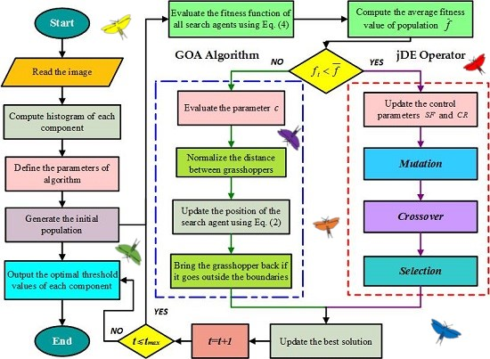
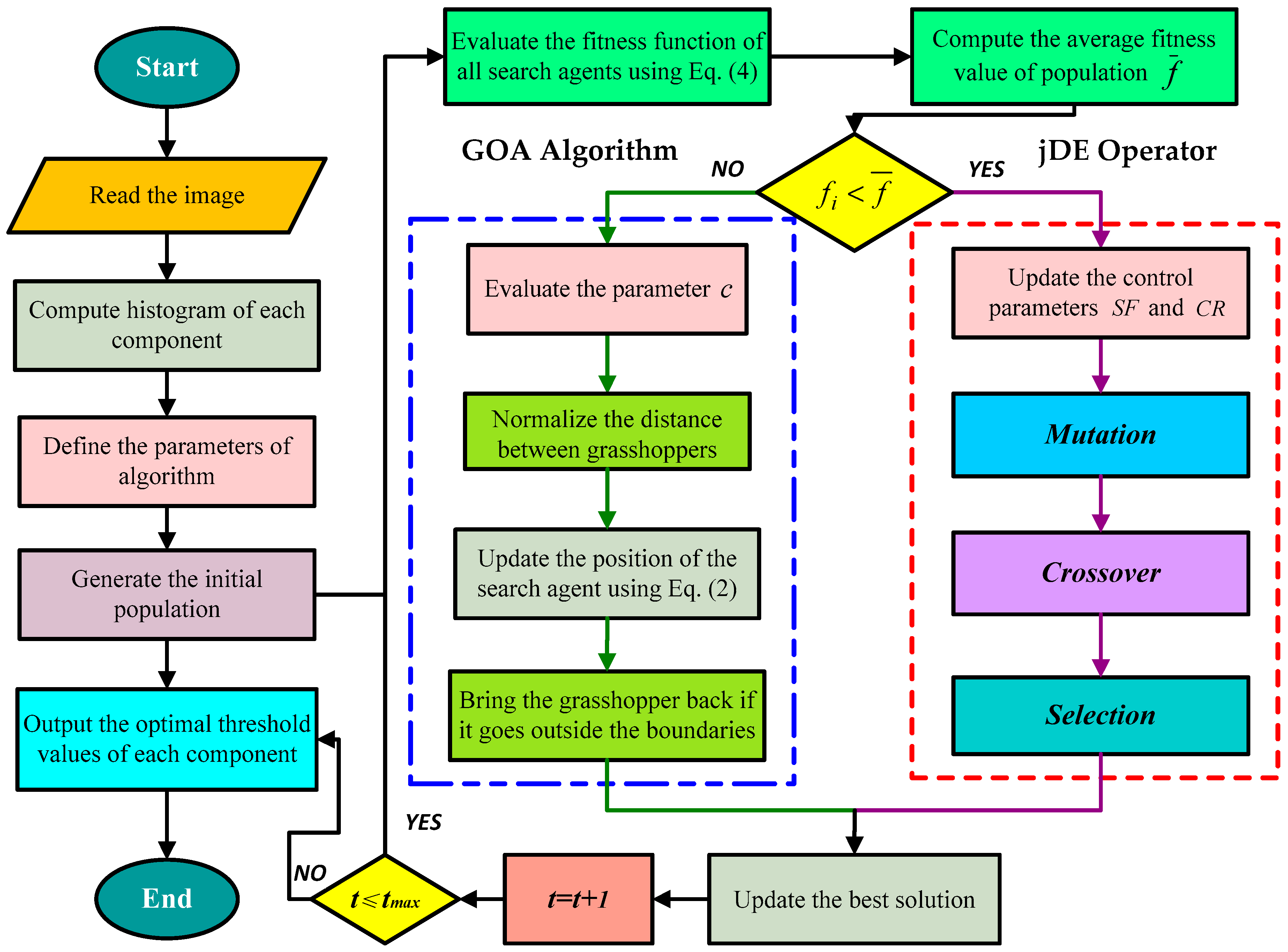
4.3. Hybrid Algorithm of GOA and jDE (GOA–jDE)

GOA is a novel meta-heuristic algorithm that has been applied to many engineering problems, however, it still has some drawbacks, such as unbalanced exploration–exploitation, sometimes slow convergence speed, and low population diversity [34,39]. DE is a simple but powerful algorithm which has been embedded into other algorithms, as an operator, to enhance local search capability. For example, Elaziz et al. introduced a moth search differential evolution (MSDE) algorithm for task scheduling in cloud computing [50]. The DE algorithm served as a local search method in MSDE, and a roulette wheel approach was used to determine which strategy would be adopted. The experimental results indicate that the proposed algorithm can efficiently solve the cloud task scheduling problem and is superior to other methods in terms of various performance measures [50]. In 2018, a hybrid algorithm based on self-adaptive gravitational search algorithm (GSA) and differential evolution was proposed, which is known as SGSADE [51]. In this paper, a DE algorithm was used with the purpose of improving the exploitation ability and maintaining population diversity [51]. The relevant simulation results demonstrate the superiority of SGSADE over other variant algorithms of GSA. In 2017, Zhao et al. presented a hybrid optimization algorithm of chaotic differential evolution and estimation of distribution [52]. The proposed algorithm, called cDE/EDA, can obtain high precision solutions due to the combination of strong exploration ability in EDA and good exploitation ability in DE.

These successful applications, using hybrid algorithm with DE, motivate us to take advantage of them to obtain a modified version of GOA. In this paper, the GOA algorithm is combined with jDE to improve search efficiency while maintaining population diversity, especially in the later iterations. It is worth noting that although the DE algorithm serves as a local search strategy in the proposed algorithm, this does not mean, however, that its exploration capability can be ignored or even discarded. After all, a good balance between exploration and exploitation is crucial for any meta-heuristic algorithm, even as part of a hybrid algorithm. Therefore, an improved version of DE, namely jDE, is used instead of the standard DE.

In the proposed GOA–jDE algorithm, a simple and efficient hybrid model is introduced to improve the optimization ability without increasing the computational complexity [53]. In the authors’ opinion, the average objective value of the population represents the overall quality of the search agents in the current generation. For a problem to be minimized, the fitness function value of individual should be less than the average, which indicates that the adjacent search region of the particle is potential and promising. Therefore, a strategy to enhance the local search should be adopted. On the contrary, if the fitness function value is greater than the average, the local search strategy will not be used. Furthermore, the introduction of jDE will not make the algorithm prematurely converge because scaling the difference between individuals makes the population more randomly distributed. This characteristic can better maintain the diversity of populations, especially in the late evolution process. Moreover, the flowchart of GOA–jDE algorithm-based multilevel thresholding is given in Figure 3, and the pseudocode is presented in Algorithm 3.

Algorithm 3 Pseudocode of GOA–jDE-based multilevel satellite image thresholding

Input: The given satellite image. Output: Segmentation thresholds. $$\begin{gathered} ********************************** \\ ** \mathrm{Get} \mathrm{information} \mathrm{about} \mathrm{the} \mathrm{image} ** \\ ********************************** \end{gathered}$$ 1. Read the given color satellite image; 2. Extract the histogram of each color component (R, G, and B); $$\begin{gathered} ********************************** \\ **** \mathrm{GOA}-\mathrm{jDE} **** \\ ********************************** \end{gathered}$$ 3. Initialize a randomly distributed population in the search space; 4. Initialize the best search agent $\widehat{T_d}$; 5. Initialize the fitness values of the grasshoppers $f_i$; 6. Set population size $N$ and maximum number of iterations $t_{\max }$; 7. Set the dimensions of the optimization problem $dim$, namely the number of thresholds; 8. while (termination condition is not met $(t<t_{\max })$) 9. Check the boundary and evaluate the fitness value of each grasshopper $f_i$ using Equation (4); 10. Update the location $\widehat{T_d}$ and fitness value $f_{\mathrm{best}}$ of best search agent if there is a better one; 11. Evaluate the parameter $c$ using Equation (3); 12. Calculate the average fitness value $\overline{f}$ of the population; 13.  for (each grasshopper $(i=1:n$)) 14.    if ($f_i>\overline{f}$)                    % GOA Algorithm 15.    Update the position of grasshopper using Equation (2); 16.    else                       % jDE Operator 17.    Evaluate $SF$ and $CR$ of each search agent using Equations (8)–(9); 18.    Mutation, Crossover, and Selection using Equations (5)–(7). 19.    end if 20.   end for 21.  end while

Fitness function (Minimum Cross entropy)

Input: Histogram of a color component, and segmentation thresholds $x_i$. Output: Fitness function value $f_i$. 1. The histogram is divided into $n+1$ parts by $n$ thresholds; 2. Calculate the proportion of pixels in each gray level $\left(p_j,j\in \left[0,255\right]\right)$ to the total based on the histogram; 3. Compute the zero-moment $m_i^0$ and first-moment $m_i^1$ on partial range of the image histogram; 4. Calculate the minimum cross entropy of each part $-m_k^1\ln \left(m_k^1/m_k^0\right)$ $\left(k\in \left[0,n\right]\right)$; 5. The sum of the entropies of all parts represents the fitness function value; 6. $f_i=-m_0^1\ln \left(m_0^1/m_0^0\right)-m_1^1\ln \left(m_1^1/m_1^0\right)-\cdots -m_n^1\ln \left(m_n^1/m_n^0\right)$;

In addition, experiments were performed on eight satellite images (see Figure 4) to determine the optimal parameter settings of the proposed algorithm. The average rank with different combinations of $SF$ and $CR$ are given in

Table 1. Average rank obtained by the proposed method (K = 12) under different parameter values.

	$\mathit{S}\mathit{F}=0.1$	$\mathit{S}\mathit{F}=0.3$	$\mathit{S}\mathit{F}=0.5$	$\mathit{S}\mathit{F}=0.7$	$\mathit{S}\mathit{F}=0.9$
$CR=0.5$	14.0625	13.75	16.6875	9.75	11.75
$CR=0.6$	7.0625	13.4375	9.8125	13	12.6875
$CR=0.7$	15.6875	16.6875	14.3125	15.1875	17.0625
$CR=0.8$	13.8125	13.8125	14.5	12.6875	9.5
$CR=0.9$	15.875	9	3	14.875	17

. Note that the values of the parameters $SF$ and $CR$ are the initial values here. Other parameters, such as ${\tau }_1$, ${\tau }_2$, etc., are the same as in the original literature [49], in which the authors have discussed, in detail, the impact of the selected parameters on the performance. In this experiment, a lower ranking value indicates better performance. As can be observed, $SF=0.5$ and $CR=0.9$ present the best results in most cases; thus, this combination of parameter values was adopted in the following experiments.

4.4. Computational Complexity

In this subsection, the computational complexity of the GOA–jDE algorithm is presented, and the details of the relevant analysis are also given.

It is worth mentioning that this paper only discusses the computational complexity in a single iteration because the number of search agents using the GOA or jDE method varies uncertainly during the evolution process. The computational complexity of the GOA–jDE and standard GOA algorithm can be calculated as follows:

$$\begin{array}{cc}O\left(\mathrm{GOA}-\mathrm{jDE}\right)& =O\left(position update\right)+O\left(objective function evaluation\right)\\ & =O\left(n_1\ast \left(d+Coc+Cos\right)+n_2\ast n\ast d+n\ast Cof\right)\\ & =O\left(n_1\ast d+n_2\ast n\ast d+n_1\ast \left(Coc+Cos\right)+n\ast Cof\right),\end{array}$$

(10)

$$\begin{array}{cc}O\left(\mathrm{GOA}\right)& =O\left(position update\right)+O\left(objective function evaluation\right)\\ & =O\left(n^2\ast d+n\ast Cof\right)=O\left({\left(n_1+n_2\right)}^2\ast d+n\ast Cof\right)\\ & =O\left(n_1{}^2\ast d+n_2{}^2\ast d+2n_1{n}_{2}d+n\ast Cof\right),\end{array}$$

(11)

where $n_1$ and $n_2$ indicate the number of search agents that update their position using jDE and GOA in one iteration, respectively. $n$ is the population size, which is equal to the sum of $n_1$ and $n_2$, namely $n=n_1+n_2$. $d$ is the dimension of given problem, $Cof$ is the cost of function evaluation. $Coc$ and $Cos$ are the cost of crossover and selection operations in DE, respectively.

It can be found, from the two above formulations, that the cost of “objective function evaluation” is equal. However, the cost of “position update” is significantly different. Therefore, only the latter needed to be analyzed to assess the differences between them. In GOA–jDE, the population is divided into two parts according to the average fitness value, while the computational complexity of these two parts is different. Mutation, crossover, and selection operations are the main costs of jDE, and the computational complexity is approximately equal to $O\left(n_1\ast \left(d+Coc+Cos\right)\right)$. For the position update using GOA, the computational complexity is approximately equal to $O\left(n_2\ast n\ast d\right)$, since each grasshopper needs to compute its social interaction, while the calculation of the distance between two individuals is essential, as shown in Equation (2). Similarly, in the GOA algorithm, the cost of the position update is equal to $O\left(n^2\ast d\right)$, which can be rewritten as $O\left({n_1}^2\ast d+{n_2}^2\ast d+2n_1{n}_{2}d\right)$. It can be seen from the final versions of Equation (10) and Equation (11) that they all contain three terms representing the cost of position update. Obviously, the first two terms of GOA–jDE cost less than the standard GOA. Considering the third term, it is difficult to determine which algorithm has higher computational complexity due to the unknown cost of crossover and selection operations represented by $Coc$ and $Cos$, respectively. In fact, the computational complexity of GOA–jDE is much lower than the standard GOA, which will be verified in subsequent experiments.

5. Experimental Results and Discussion

5.1. Experimental Setup

In this paper, a series of experiments are conducted to validate the performance of GOA–jDE algorithm, which can be mainly divided into three parts. For the first experiment, eight satellite color images are selected from “Landsat imagery courtesy of NASA Goddard Space Flight Center and U.S. Geological Survey” [54]. It is worth noting that all images are resized, and the height is fixed to 481 pixels. Both state-of-the-art and conventional multilevel color image segmentation techniques are employed, such as the standard GOA and DE, modified GOA (MGOA) [55], hybrid jDE (hjDE) [21], $\mathsf{\beta }$DE (BDE) [56], bat algorithm (BA) [17], and particle swarm optimization (PSO) [15]. For the second experiment, the GOA–jDE-based method using MCE (GOA–jDE–MCE) with other threshold-based satellite image segmentation methods, such as modified artificial bee colony using Tsallis entropy (MABC–Tsallis) [57], improved the differential search algorithm using Otsu between-class variance (IDSA–Otsu) [58], and cuckoo search using MCE (CS–MCE) [13]. Considering that these methods use different thresholding techniques, the GOA–jDE algorithm was combined with Tsallis entropy and Otsu methods for fair comparison, and the resulting two techniques were named GOA–jDE–Tsallis and GOA–jDE–Otsu. For the third experiment, the SIPI Image Database (37 color satellite images and 1 grayscale satellite image) was used for further testing [59].

Hence, the performance of each approach can be comprehensively evaluated through the above experiments. In addition, Figure 4 presents the original satellite image and corresponding histogram. The images are named in order (i.e., “Image1” to “Image8”), and the relevant explanation is given in

Table 2. Explanation of the satellite images.

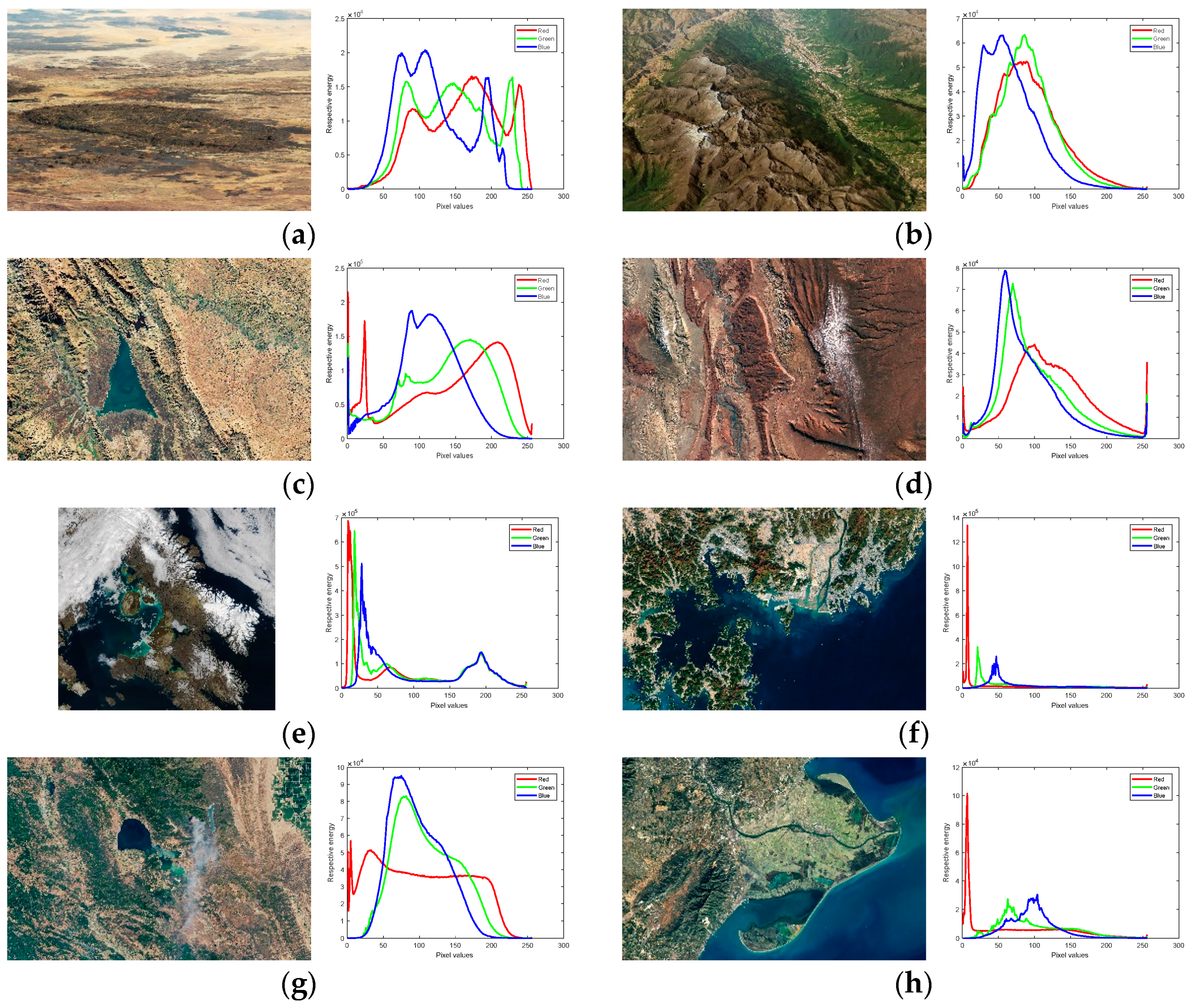
Image Number	Explanation
1.	The Aïr Mountains dispersed across the Sahara Desert in northern Niger.
2.	Glacier cover in the mountainous region of northwestern Venezuela.
3.	Dukan Lake in the Zagros Mountains, the largest lake in Iraqi Kurdistan.
4.	Candeleros rock containing quite a menagerie of fossilized fauna.
5.	The waters of Foxe Basin, which have been choked with sea ice for most of the year.
6.	The Port of Busan at the southeastern tip of the Korean Peninsula, which has been a trading hub since at least the 15th century.
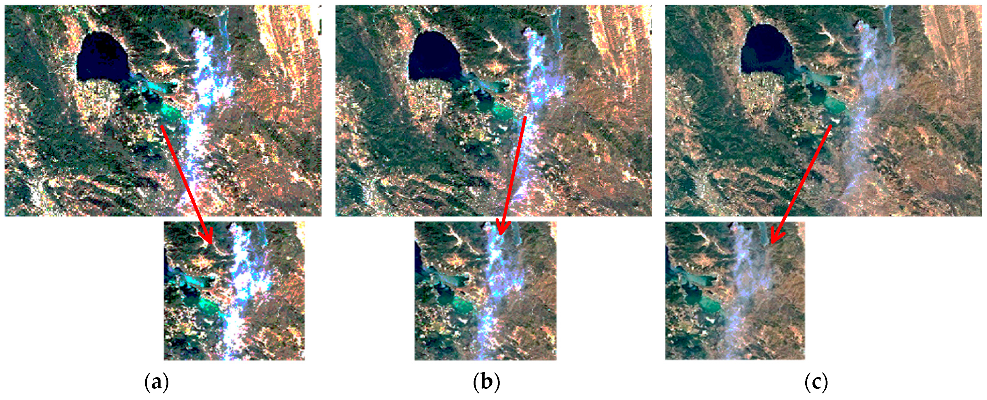
7.	A fire in Northern California during the summer of 2018.
8.	The Ebro Delta, located more than 200 kilometers (120 miles) southwest of Barcelona.

.

The parameter values were set according to the original literature, as shown in

Table 3. Parameters of the algorithms.

No.	Algorithm	Parameter Setting	Year	Reference
1.	GOA–jDE	$CR=0.9,SF=0.5,S{F}^{low}=0.1,S{F}^{up}=0.9,{\tau }_1={\tau }_2=0.1$	—	—
2.	GOA	$c\in \left[0.00001,1\right]$	2017	[33]
3.	DE	$CR=0.9,SF=0.5$	1997	[16]
4.	MGOA	$\beta =0.8 \left(\mathrm{L}é\mathrm{vy} \mathrm{flight} \mathrm{parameter}\right)$	2019	[55]
5.	hjDE	$p_a=0.25 \left(\mathrm{switching} \mathrm{probability}\right)$	2016	[21]
6.	BDE	$a\in \left[0,1\right] \left(\mathrm{beta} \mathrm{distribution} \mathrm{parameter}\right)$	2018	[56]
7.	BA	$r_i\in \left[0,1\right] \left(\mathrm{rate} \mathrm{of} \mathrm{pulse} \mathrm{emission}\right),A_i\in \left[1,2\right] \left(\mathrm{loudness} \mathrm{value}\right)$	2010	[17]
8.	PSO	$c_1=c_2=2,w\in \left[0.4,0.9\right],v_{max}=25.5$	1995	[15]
9.	MABC	$K=300 \left(\mathrm{chaotic} \mathrm{iteration}\right)$	2015	[57]
10.	IDSA	—	2018	[58]
11.	CS	$p_a=0.25 \left(\mathrm{mutation} \mathrm{probability}\right), \beta =1.5 \left(\mathrm{scalingfactor}\right)$	2017	[13]

, except for the population size $N$, set to 30, and the number of iterations $t_{\max }$, set to 500 for fair comparison. All experiments were performed 30 times to eliminate errors, and the best result in each case is highlighted in boldface. The experimental environment is given as follows: MATLAB 2017 and Microsoft Windows 10 operating system.

5.2. Performance Measures

In this section, several quantitative indicators are introduced to evaluate the performance of algorithms, such as average fitness values, standard deviation (STD), peak signal to noise ratio (PSNR), structural similarity index (SSIM), and feature similarity index (FSIM), as well as Wilcoxon’s rank sum test and Friedman test. The description of these metrics can be found in

Table 4. Performance measures of the multilevel image segmentation methods.

No.	Measures	Formulation	Remark	Reference
1.	Average Fitness Function Value	$\mathrm{Average}=\frac{{\sum }_{i=1}^N{f}_i}{N}$	Indicates the center value of sample data.	[46]
2.	Standard Deviation (STD)	$\mathrm{Std}=\sqrt{\frac{1}{N-1}{{\displaystyle \sum }}_{i=1}^N{\left(f_i-\mathrm{Average}\right)}^2}$	Reflects the degree of dispersion in a dataset. A lower value shows better performance.	[46]
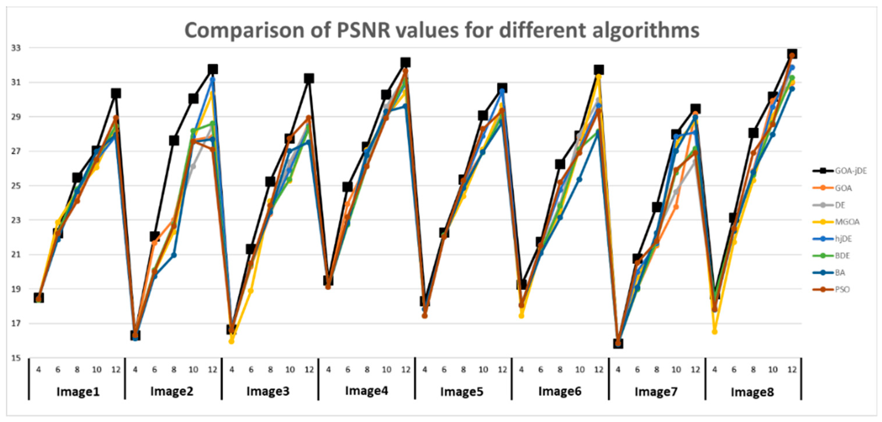
3.	Peak Signal to Noise Ratio (PSNR)	$\mathrm{PSNR}=10{\log }_{10}\left(\frac{{255}^2}{\mathrm{MSE}}\right)$	The ratio of the maximum possible power of the signal to the destructive noise power.	[60]
4.	Mean Squared Error (MSE)	$\mathrm{MSE}=\frac{1}{MN}{{\displaystyle \sum }}_{i=1}^M{{\displaystyle \sum }}_{j=1}^N{\left[I\left(i,j\right)-K\left(i,j\right)\right]}^2$	Computes the difference between the predicted value.	[60]
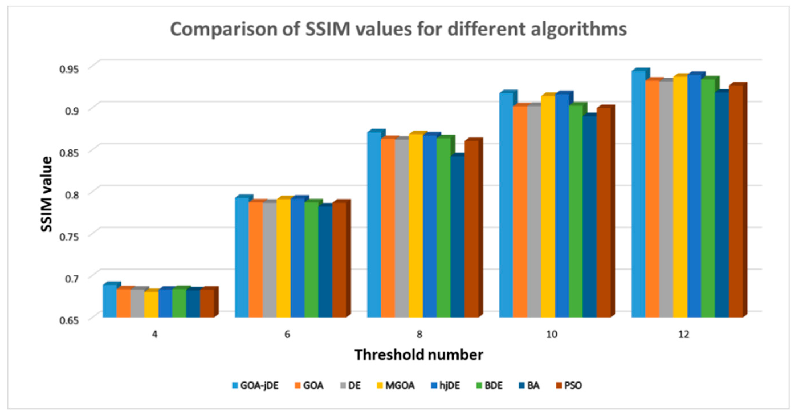
5.	Structural Similarity Index (SSIM)	$\mathrm{SSIM}=\frac{\left(2{\mu }_x{\mu }_y+c_1\right)\left(2{\sigma }_{xy}+c_2\right)}{\left({\mu }_x^2+{\mu }_y^2+c_1\right)\left({\sigma }_x^2+{\sigma }_y^2+c_2\right)}$	Defines the similarity between the original image and the segmented image.	[61]
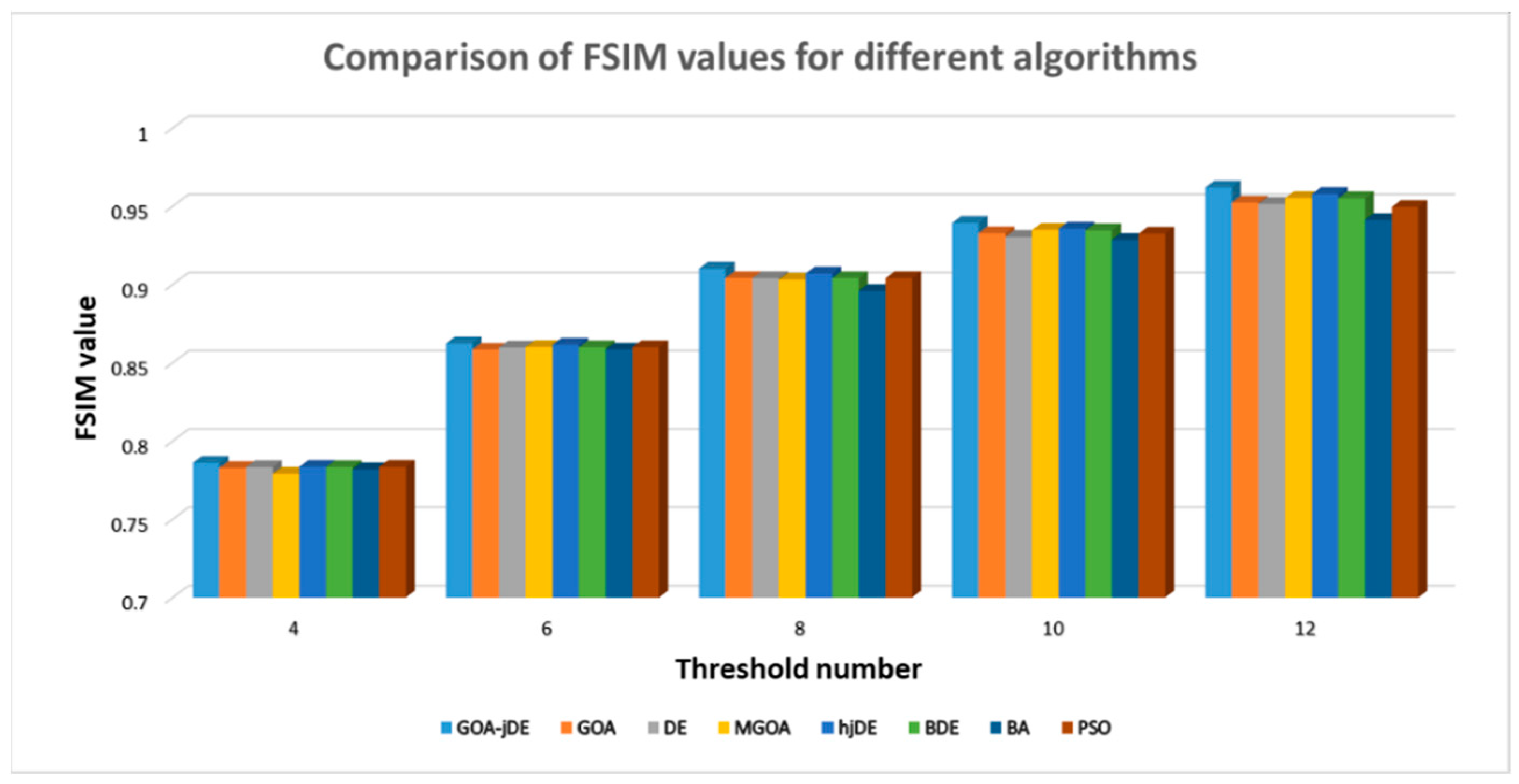
6.	Feature Similarity Index (FSIM)	$\mathrm{FSIM}=\frac{{\sum }_{x\in \Omega }{S}_L\left(x\right)·P{C}_m\left(x\right)}{{\sum }_{x\in \Omega }P{C}_m\left(x\right)}$	Reflects the similarity of feature structure, the maximum value is 1.	[62]
7.	Average Computation Time	$Time=\frac{{\sum }_{i=1}^{N}tim{e}_i}{N}$	Indicates the operating efficiency of each method.	[14]
8.	Wilcoxon’s Rank Sum Test	$$\begin{gathered} R^{+}={\displaystyle {\displaystyle \sum }_{d_i>0}}rank\left(d_i\right)+\frac{1}{2}{\displaystyle {\displaystyle \sum }_{d_i=0}}rank\left(d_i\right) \\ {R}^{-}={\displaystyle {\displaystyle \sum }_{d_i<0}}rank\left(d_i\right)+\frac{1}{2}{\displaystyle {\displaystyle \sum }_{d_i=0}}rank\left(d_i\right) \end{gathered}$$	Whether there is a significant difference between two algorithms.	[63]
9.	Friedman Test	$F_f=\frac{12n}{k\left(k+1\right)}\left[{{\displaystyle \sum }}_j{R}_j^2-\frac{k{\left(k+1\right)}^2}{4}\right]$	Detects significant differences between the behaviors of two or more algorithms.	[64]

.

Furthermore, another performance metric called segmentation success rate (SSR) is introduced in this paper, which takes PSNR, SSIM, and FSIM indexes into consideration for comprehensively measuring the similarity between the segmented image and the original image. SSR determines how many times the technique successfully reached a specified value that is called value-to-reach (VTR):

$$SR=\frac{NVTR}{total number of runs},$$

(12)

where $NVTR$ is the number of times that the technique reached the $VTR$.

5.3. Experimental Series 1: Comparison of Satellite Image Thresholding Methods Based on MCE

5.3.1. Results and Discussions

The experimental results can be found in

Table 5. The average fitness values using the MCE method compared with other algorithms.

Images	K	GOA–jDE	GOA	DE	MGOA	hjDE	BDE	BA	PSO
Image1	4	−701.0136	−700.9701	−701.0136	−701.0136	−701.0136	−701.0136	−701.0132	−701.0136
	6	−701.2706	−701.2705	−701.2705	−701.2705	−701.2706	−701.2704	−701.2267	−701.2702
	8	−701.3808	−701.3829	−701.3803	−701.3806	−701.3807	−701.3807	−701.3152	−701.3782
	10	−701.4401	−701.4371	−701.4395	−701.4389	−701.4392	−701.439	−701.3746	−701.4042
	12	−701.4753	−701.473	−701.4737	−701.4736	−701.4751	−701.4749	−701.3678	−701.4573
Image2	4	−370.8833	−370.8833	−370.8833	−370.8833	−370.8833	−370.8833	−370.7795	−370.8833
	6	−371.1958	−371.1958	−371.1959	−371.1958	−371.1959	−371.1959	−371.045	−371.1898
	8	−371.3386	−371.3108	−371.3372	−371.3209	−371.3385	−371.3381	−371.2998	−371.2486
	10	−371.4126	−371.3998	−371.4082	−371.3839	−371.4124	−371.4115	−371.2348	−371.3697
	12	−371.457	−371.4345	−371.4507	−371.4395	−371.4569	−371.4558	−371.3314	−371.3988
Image3	4	−645.6498	−645.6498	−645.6498	−645.6498	−645.6498	−645.6498	−645.646	−645.6498
	6	−646.008	−645.9872	−646.008	−646.008	−646.008	−646.0079	−645.98	−646.0059
	8	−646.1744	−646.1662	−646.1735	−646.1743	−646.1742	−646.1741	−646.066	−646.1298
	10	−646.261	−646.2592	−646.2597	−646.2605	−646.2603	−646.2582	−646.1845	−646.235
	12	−646.3107	−646.2853	−646.3092	−646.3039	−646.3077	−646.3098	−646.2148	−646.2988
Image4	4	−474.0258	−474.0258	−474.0257	−474.0258	−474.0258	−474.0254	−474.0241	−474.0257
	6	−474.3694	−474.3683	−474.3691	−474.3694	−474.3694	−474.3693	−474.3543	−474.3685
	8	−474.526	−474.5238	−474.5229	−474.5259	−474.5251	−474.5257	−474.3738	−474.5036
	10	−474.6101	−474.6052	−474.6082	−474.6068	−474.6088	−474.6082	−474.4214	−474.5932
	12	−474.6598	−474.6508	−474.6569	−474.6563	−474.6596	−474.6585	−474.5078	−474.6356
Image5	4	−498.1325	−498.1325	−498.1325	−498.1325	−498.1325	−498.1325	−498.1271	−498.1325
	6	−498.5083	−498.4884	−498.5083	−498.5083	−498.5082	−498.4757	−498.4172	−498.5078
	8	−498.6791	−498.6698	−498.6783	−498.6784	−498.6791	−498.679	−498.5085	−498.6742
	10	−498.774	−498.7722	−498.7672	−498.7733	−498.7731	−498.7736	−498.6267	−498.734
	12	−498.8269	−498.8226	−498.8201	−498.826	−498.8248	−498.826	−498.7248	−498.8073
Image6	4	−306.5464	−306.5464	−306.5463	−306.5464	−306.5464	−306.5461	−306.5389	−306.5463
	6	−306.9244	−306.9237	−306.9244	−306.9244	−306.9244	−306.9231	−306.8676	−306.8951
	8	−307.0986	−307.0977	−307.0981	−307.0985	−307.0985	−307.0985	−306.8234	−307.0793
	10	−307.1962	−307.187	−307.1699	−307.1871	−307.1961	−307.1912	−307.0848	−307.1482
	12	−307.2547	−307.2322	−307.2507	−307.2423	−307.252	−307.2517	−307.0775	−307.2106
Image7	4	−480.5483	−480.5483	−480.5483	−480.5483	−480.5483	−480.5483	−480.5475	−480.548
	6	−480.8448	−480.8428	−480.8441	−480.8448	−480.8448	−480.8448	−480.7985	−480.8158
	8	−480.974	−480.9729	−480.9725	−480.9735	−480.9733	−480.9725	−480.83	−480.9581
	10	−481.041	−481.0396	−481.0402	−481.04	−481.0408	−481.0407	−480.9169	−481.0313
	12	−481.0802	−481.0699	−481.0776	−481.0723	−481.0796	−481.0771	−480.9164	−481.0549
Image8	4	−411.1164	−411.1164	−411.1164	−411.1164	−411.1164	−411.1164	−411.1118	−411.1164
	6	−411.4617	−411.4605	−411.4616	−411.4616	−411.4616	−411.4611	−411.308	−411.4607
	8	−411.6287	−411.6273	−411.6285	−411.6284	−411.6286	−411.6231	−411.5499	−411.5935
	10	−411.7136	−411.7007	−411.7105	−411.7043	−411.7119	−411.7131	−411.6203	−411.6984
	12	−411.7664	−411.7632	−411.7641	−411.758	−411.7662	−411.7653	−411.6613	−411.7395

,

Table 6. The SSR values using MCE method compared with other algorithms.

Images	GOA–jDE	GOA	DE	MGOA	hjDE	BDE	BA	PSO
1	6.67	0	0	0	0	0	3.33	0
2	100	0	10	86.67	0	0	36.67	13.33
3	83.33	26.67	20	40	0	23.33	0	10
4	100	100	100	96.67	100	93.33	100	90
5	0	0	0	0	0	0	0	0
6	100	60	36.67	53.33	30	70	86.67	40
7	73.33	0	3.33	40	0	6.67	13.33	0
8	100	100	100	100	100	100	100	100

,

Table 7. The average CPU time of the MCE method at different threshold levels.

K	GOA–jDE	GOA	DE	MGOA	hjDE	BDE	BA	PSO
4	1.744575	3.339125	1.132188	3.338625	1.632425	1.50965	1.3265	1.081413
6	1.814575	3.407225	1.225213	3.467038	1.734113	1.701825	1.5425	1.1903
8	2.027638	3.493013	1.31005	3.492675	1.987663	1.876263	1.885988	1.321688
10	2.258513	3.567325	1.446075	3.58	2.248538	2.023563	2.240663	1.454863
12	2.558875	3.860313	1.5924	3.750038	2.380238	2.263163	2.813125	1.56585

,

Table 8. The p-value (Wilcoxon rank sum test) for the experimental results of the MCE method.

Comparison	p-Value
GOA–jDE vs. GOA	0.0197
GOA–jDE vs. DE	2.7461 × 10−4
GOA–jDE vs. MGOA	2.3012 × 10−5
GOA–jDE vs. hjDE	8.7216 × 10−4
GOA–jDE vs. BDE	1.6063 × 10−9
GOA–jDE vs. BA	3.9766 × 10−7
GOA–jDE vs. PSO	5.0219 × 10−8

and

Table 9. The average rank (Friedman test) for the experimental results of the MCE method.

K	Average Rank
	GOA-jDE	GOA	DE	MGOA	hjDE	BDE	BA	PSO
4	2	5.4625	3.6	4.55	4.075	4.9	6.4125	5
6	1.475	5.425	4.1	4.3375	3.75	4.9625	6.7625	5.1875
8	1.0625	4.6125	4.4125	4.475	4.325	4.725	6.9625	5.425
10	1.05	4.8625	4.8125	4.6375	3.7625	4.2125	6.9625	5.7
12	1	5.0375	4.2375	4.5875	3.725	4.3875	7.5125	5.5125

and Figure 5, Figure 6, Figure 7, Figure 8, Figure 9, Figure 10 and Figure 11. Figure 5 and Figure 6 give the segmented results of “Image4” and “Image7” at different threshold levels, respectively. It can be found, from the figures, that the segmented images using high threshold levels contain more detail and information than those using low threshold levels. To be more specific, the local zoom map of “Image4” illustrates that the segmentation operation of higher dimensions makes the texture of the rock clearer. On the contrary, in the case of lower threshold, the given image is only divided into a few classes, which cannot reflect much of the image information, resulting in a poor segmentation effect. Considering the segmentation of “Image7”, it can be found that the lower threshold mistakenly classifies the fire source and the smoke, as their gray levels are relatively close (but not the same); when K = 12, the effect is improved because a segmentation threshold between the two gray levels is obtained. The reason for all the above phenomena is that as the number of threshold values increase, more classes with different characteristics are acquired, which can maintain the local features of the original image. In fact, it is difficult for the human eye to determine the performance of each algorithm at the same threshold level, especially the complex image with multiple objects. Therefore, the quality of the segmented images needs to be further evaluated using some specific indicators.

Table 5 presents the average objective function (minimum cross entropy) value obtained by each algorithm over all satellite images (bolded results are best). Note that a lower function value indicates better performance. It can be seen from the table that the proposed method presents the lowest value in most cases. For example, under the conditions of “Image3” (for K = 12), the fitness values are −646.3107, −646.2853, −646.3092, −646.3039, −646.3077, −646.3098, −646.2148, and −646.2988 for GOA–jDE, GOA, DE, MGOA, hjDE, BDE, BA, and PSO, respectively. It is obvious that GOA–jDE outperforms the compared algorithms, indicating its remarkable optimization ability and balanced exploration–exploitation. At the same time, this convincingly demonstrates that the segmented image obtained by the proposed approach is detailed, informative, and of high quality because the entropy of a given image indicates its average information content [65]. More specifically, the reason for the high precision is the use of a powerful hybrid model. In GOA–jDE, the whole population is divided into two parts according to the average fitness value. Compared to the standard GOA and DE, the exploration and exploitation stages of optimization are well balanced, which increases the probability of obtaining the global optimum. Compared to other algorithms, the GOA–jDE algorithm can maintain the population diversity in the late iteration, thus enhancing the ability to avoid local optimization. For example, the main drawback of PSO is the parameter $\omega$. If the starting and ending value of parameter $\omega$ for the current problem are not determined in the best form, the PSO may converge prematurely and fall into a local optimum. For the BA algorithm, more parameters need to be adjusted for different problems, such as $r_i$ (rate of pulse emission), $A_i$ (loudness value), and $v_{\max }$ (maximum velocity). The determination of these parameters greatly reduces the universality of BA algorithm, which affects the performance to some extent.

Moreover, the convergence property is also an indicator for evaluating the performance of each algorithm. Some typical drawbacks of the meta-heuristic algorithm can be analyzed from the convergence curve, including premature convergence and slow convergence speed. The convergence curve of each algorithm on “Image2”, “Image4”, “Image6”, and “Image8” at 12 threshold levels is shown in Figure 7 because the difference between algorithms is obvious at a higher threshold. It can be observed from the results that, in most cases, the GOA–jDE algorithm performs better than other methods. In other words, the curve given by the proposed algorithm is relatively low, overall. As discussed above, the main disadvantages of GOA are slow convergence speed and unbalanced exploration–exploitation, which are reflected clearly in the curves. For instance, under the conditions of “Image8”, it can be observed that the optimal value obtained by the GOA is continuously updated throughout the iterative process, showing no tendency to converge. This phenomenon illustrates the slow convergence drawback of GOA. However, the GOA–jDE algorithm can better balance the exploration and exploitation stages, showing neither premature convergence nor slow convergence. In fact, the superiority of the proposed algorithm is not only reflected in the segmentation task of “Image8”, but also in other images. The promising result indicates the remarkable performance of GOA–jDE, which is suitable for the problem of satellite image segmentation.

Figure 8, Figure 9 and Figure 10 present the PSNR, SSIM, and FSIM values obtained by all algorithms, respectively. As discussed above, the combination of thresholds determines the quality of segmented images, which is reflected in the indicator value of the experiment. A higher value means more similarity to the original image. It can be found, from the figure, that the value of the PSNR indicator increases as the number of thresholds increases, and the position of the line graph given by the proposed method is significantly higher than the compared algorithms, except for “Image5”. The reason for this phenomenon is that each image corresponds to a different optimization problem, and it is difficult to find a single algorithm that is universally applicable. Therefore, GOA–jDE can still be considered efficient and powerful from a holistic perspective, although it does not give the best results in all cases. Considering the SSIM and FSIM values obtained over all available images at 12 threshold levels, the algorithms can be ranked, in our study, as GOA–jDE > hjDE > BDE ~ MGOA > GOA > DE > PSO > BA. When the threshold level is low (K = 4 and 6), the difference between the algorithms is not obvious, while the difference becomes significant at high threshold levels (K = 12). Table 6 gives the SSR values obtained by each method at 12 threshold levels. Note that the specified values of PSNR, SSIM, and FSIM, here, are 29.5, 0.93, and 0.95 respectively, which is a good reflection of the performance differences between the algorithms in this study. It can be found that GOA–jDE-based technique shows excellent performance in “Image 3” and “Image 7” (i.e., its advantages are obvious). Considering “Image 5”, although each algorithm does not achieve the expected results, it can be found from Figure 8, Figure 9 and Figure 10 that the proposed method is relatively advantageous. The performance of GOA–jDE benefits from its accurately determined threshold and the resulting high-quality segmented image. On the contrary, several compared algorithms, such as DE, BA, and PSO, could not obtain the ideal segmented images due to improper determination of the threshold, and the similarity with the original image is not high.

Due to the random property of the meta-heuristic algorithm, it was necessary to perform detailed stability analysis. Boxplots were used to evaluate the stability of each algorithm. The relevant results of four randomly selected images can be seen in Figure 11. It can be observed that the proposed method again outperforms the others. More specifically, the boxplot obtained was lower in position, more compact, and had no bad points, indicating better stability, continuity, and consistency. However, the performance of the other algorithms was not ideal. For example, considering the segmentation of “Image8”, the data presented by BA fluctuate greatly, and the center of the boxplot was obviously higher than other algorithms, showing poor stability. Moreover, in the conditions of “Image7”, BDE gives a low median and relatively compact graph, but its accuracy is seriously affected by the existence of bad points. After all, algorithms with unstable performance are difficult to apply to practical engineering problems. In GOA–jDE, a powerful hybrid model was used to balance the exploration and exploitation stages. Thus, its performance was not greatly affected by the random characteristic of the meta-heuristic algorithm, showing remarkable stability in most cases.

Time complexity is also an important indicator for evaluating the performance of meta-heuristic algorithms. In engineering practices, high-precision but high-complexity algorithms are often not the best choice, but algorithms that are fast and can obtain approximate optimal solutions are generally used. Hence, the standard for measuring an algorithm cannot be just computation time or precision and, instead, the evaluation should be comprehensive and objective. The average CPU time of each algorithm can be found in Table 7. It can be observed that PSO is the fastest among available algorithms, but it cannot achieve the best values of the above indicators. The DE algorithm gives competitive results in some cases and is slightly slower than PSO in the overall consideration. In addition, the computation time of GOA–jDE is between GOA and DE, which is determined by the used hybrid model. It is worth noting that this result does not mean that the proposed algorithm is inefficient. As discussed above, the evaluation of algorithm performance should be more comprehensive and objective. The proposed algorithm has shown remarkable performance in many aspects, despite not being the fastest. In summary, GOA–jDE is a high-performance algorithm which can improve the precision significantly while maintaining runtime. Furthermore, the proposed algorithm has a few adjustable parameters, which enables it to adapt to the segmentation of most images. After all, tuning the algorithm parameters may be more complicated than optimizing the problem itself [25].

5.3.2. Statistical Tests

Since the experiments of all available methods were the same, it was necessary to perform statistical tests. Friedman test [64] and Wilcoxon’s rank sum test [63] were used as non-parametric statistical tests for evaluating the performance of all algorithms, with 5% considered as the significant level. The null hypothesis $\left({\mathrm{H}}_0\right)$ in Wilcoxon’s rank sum test assumes that there is no significant difference between the two algorithms being compared, and the alternative hypothesis $\left({\mathrm{H}}_1\right)$ indicates the difference. In addition, ${\mathrm{H}}_0$ in the Friedman test states the equality of medians between the algorithms, while ${\mathrm{H}}_1$ also indicates the difference. A more detailed description of Friedman test and Wilcoxon’s rank sum test can be found in the literature [66].

The experimental results can be seen in three tables. From Table 8, the proposed method gives better results (p < 0.05 and h = 1) in all cases, which indicates that the indicator values given by GOA–jDE are not appearing randomly. For the Friedman test, it is worth mentioning that calculating the rankings is the first step, the relevant results of which are presented in Table 9. It can be found from the table that the proposed method ranks first in all cases. The chi-square $\left({\chi }^2\right)$ value and p-value are presented in

Table 10. The chi-square value and p-value (Friedman test) for the experimental results of the MCE method.

K	Chi-Square Value	p-Value
4	101.901	4.36751 × 10−19
6	114.919	8.73960 × 10−22
8	126.529	3.33534 × 10−24
10	135.448	4.56229 × 10−26
12	155.666	2.61739 × 10−30

. According to the chi-square distribution table, the critical value for 7 (8 algorithms − 1) degrees of freedom with 5% significant level is 14.067 [67,68]. As shown in Table 10, the chi-square values obtained at all threshold levels were much larger than the critical value, and the p-values acquired for all number of thresholds were far less than 0.05. This promising result indicates that ${\mathrm{H}}_0$ can be rejected in all cases, and there is a significant difference among the algorithms. The experiments in this section demonstrate the statistical significance of the performance of GOA–jDE algorithm.

5.4. Experimental Series 2: Performance on Other Objective Functions

In this section, the GOA–jDE–MCE method is compared with other advanced satellite image thresholding methods, such as MABC–Tsallis [57], IDSA–Otsu [58], and CS–MCE [13]. Considering the different criteria used in each method, the GOA–jDE algorithm was combined with MCE, Tsallis entropy, and Otsu’s method for fair comparison. In other words, three sets of comparisons were performed, namely GOA–jDE–Tsallis versus MABC–Tsallis, GOA–jDE–Otsu versus IDSA–Otsu, and GOA–jDE–MCE versus CS–MCE. The selected performance measure was the average objective function value. Furthermore, two natural images from the Berkeley segmentation dataset were also used to test the robustness of the algorithm, which are given in Figure 12 [69]. It is worth noting that higher threshold levels (20, 25, and 30) were adopted in this experiment because the satellite images contained more information and detail than normal images. More critically, the objects (targets) that needed to be determined and segmented were, in general, multiple and varied [70]. Therefore, in this section, the threshold level was increased to assess the algorithm performance more practically.

Table 11. Average objective function value obtained using Tsallis entropy, Otsu’s method, and MCE.

Images	K	Tsallis		Otsu		MCE
		GOA–jDE	MABC	GOA–jDE	IDSA	GOA–jDE	CS
Image1	20	65.6992	63.9303	2536.0239	2533.7508	−701.5320	−701.5321
	25	72.0775	69.8990	2538.4352	2537.4078	−701.5441	−701.5440
	30	78.0006	74.2769	2540.1262	2539.0127	−701.5516	−701.5513
Image2	20	65.1949	63.3661	1380.4683	1378.9008	−371.5264	−371.5240
	25	71.4121	69.0462	1382.6497	1382.0753	−371.5386	−371.5390
	30	77.1012	73.8485	1383.9328	1383.0637	−371.5467	−371.5457
Image3	20	66.3283	64.7228	2267.4996	2265.5258	−646.3892	−646.3875
	25	73.0784	70.6841	2270.3662	2269.1050	−646.4058	−646.4052
	30	78.9913	74.9226	2272.1397	2270.5508	−646.4160	−646.4150
Image4	20	67.2077	65.8090	1654.2822	1652.9518	−474.7376	−474.7383
	25	74.0556	71.2441	1656.8361	1655.9701	−474.7543	−474.7542
	30	80.2195	75.7998	1658.3974	1657.8302	−474.7638	−474.7638
Image5	20	67.1305	65.6002	5516.8189	5515.3632	−498.9233	−498.9223
	25	74.3413	71.3003	5519.9728	5519.1290	−498.9440	−498.9433
	30	79.8769	75.9055	5521.8659	5521.0078	−498.9556	−498.9552
Image6	20	66.7823	65.4021	3210.8833	3209.5405	−307.3492	−307.3459
	25	74.1973	71.5457	3213.7465	3212.8257	−307.3670	−307.3685
	30	79.4842	75.5905	3215.0132	3214.2657	−307.3798	−307.3795
Image7	20	65.5192	63.8334	1803.2208	1801.3177	−481.1434	−481.1416
	25	72.4605	68.99	1805.3468	1803.8873	−481.1571	−481.1556
	30	77.5298	74.1611	1806.9075	1806.2681	−481.1634	−481.1624
Image8	20	66.8490	65.1504	2355.6389	2354.3242	−411.8501	−411.8497
	25	73.6971	71.5997	2358.1153	2356.7401	−411.8686	−411.8674
	30	78.9075	75.0792	2359.6548	2358.5339	−411.8757	−411.8768
Elephant	20	62.1191	60.7010	2009.5697	2008.3336	−457.3469	−457.3467
	25	67.8767	66.4680	2011.4073	2010.5957	−457.3577	−457.3569
	30	72.9363	69.5792	2012.2340	2011.6498	−457.3633	−457.3631
Plane	20	52.1894	52.1762	706.7254	706.6974	−587.0459	−587.0450
	25	55.6713	55.8603	707.6530	707.4842	−587.0525	−587.0503
	30	58.7978	58.3922	707.8326	708.1450	−587.0541	−587.0538

gives the average objective function value obtained by each thresholding technique (bolded results are best). In the comparison with MABC–Tsallis, the GOA–jDE algorithm exhibits a remarkable performance based on the Tsallis entropy thresholding technique, which is reflected in all the obtained values. Moreover, considering the experiment on natural images, GOA–jDE–Tsallis presents better results in most cases, indicating the robustness and universality of the algorithm. For the comparison with the other two methods, it can be seen that the proposed algorithm-based methods are, again, superior to other methods. In general, the compared method based on MCE is relatively more competitive than the compared method based on Tsallis entropy and Otsu’s method, because the first one gives better results in more cases.

5.5. Experimental Series 3: Further Evaluation on SIPI Image Database

In this section, the performance of the proposed algorithm is further verified on the SIPI Image Database (37 color satellite images and 1 grayscale satellite image). The experiment was carried out at high threshold levels, which are the same as in Section 5.4. Note that the compared selected algorithms are based on different criteria, thus, the PSNR, SSIM, and FSIM indicators are utilized instead of average fitness values.

Table 12. Average rank of the results for each algorithm on the SIPI Image Database.

K	Average Rank
	GOA–jDE–MCE	MGOA–MCE	hjDE–MCE	BDE–MCE	BA–MCE	PSO–MCE	CS–MCE	IDSA–Otsu	MABC–Tsallis
20	3.1754	4.4781	5.5833	6.3070	5.6974	4.9693	4.9167	3.9430	5.9298
25	2.7368	4.9342	5.0746	6.5219	6.4342	4.1535	4.8640	4.2588	6.0219
30	1.3421	4.6886	4.5526	5.9254	7.4386	5.1798	4.6316	4.5175	6.7237
Overall	2.4181	4.7003	5.0702	6.2515	6.5234	4.7675	4.8041	4.2398	6.2251

presents the average rank of the results for each algorithm. A lower ranking value indicates better performance. It can be found that the GOA−jDE ranks first in all cases, and the advantage is more obvious at higher threshold levels (K = 30). Another interesting result is that the MCE method is more competitive than the Tsallis entropy thresholding technique in the field of satellite image segmentation. More specifically, the results of MABC–Tsallis are not superior to those of MCE-based approaches. However, this does not mean that the methods based on Tsallis entropy are inefficient or meaningless. As stated in the no free lunch (NFL) theorem [71], no algorithm can solve all engineering problems. GOA–jDE–Otsu and GOA–jDE–Tsallis thresholding methods may exhibit superior performance in other image segmentation fields, including CT and MR images. Therefore, applications of the proposed algorithm are potential and meaningful.

6. Conclusions

In this paper, a novel hybrid GOA with DE is proposed for multilevel satellite image segmentation. MCE is used to select the segmentation thresholds. The proposed algorithm, known as GOA–jDE, can search the solution space more efficiently and present the segmented image with higher quality than the standard GOA and DE. A series of experiments were carried out on various satellite images to evaluate the performance of the proposed method. Both the standard multilevel color image thresholding methods and the advanced multilevel satellite image thresholding methods were used for comparison, such as MABC–Tsallis, IDSA–Otsu, CS–MCE, and others. Comprehensive statistical tests, including Friedman test and Wilcoxon’s rank sum test, were also performed to assess the significant differences between the methods. Furthermore, natural images from the Berkeley segmentation dataset were selected to validate the strong robustness of GOA–jDE–MCE. The experimental results indicate that the proposed satellite image segmentation method outperforms other compared approaches, which has broad application prospects and potential. In future, several recently proposed meta-heuristic algorithms, such as Harris hawks optimization, seagull optimization algorithm, and the sailfish optimizer will be introduced into the field of image segmentation. Magnetic resonance (MR) images and computed tomography (CT) images will also be considered for testing.

References

- Hinojosa, S.; Dhal, K.G.; Elaziz, M.A.; Oliva, D.; Cuevas, E. Entropy-based imagery segmentation for breast histology using the stochastic fractal search. Neurocomputing 2018, 321, 201–215. [Google Scholar] [CrossRef]
- Elaziz, M.A.; Oliva, D.; Ewees, A.A.; Xiong, S. Multi-level thresholding-based grey scale image segmentation using multi-objective multi-verse optimizer. Expert Syst. Appl. 2019, 125, 112–129. [Google Scholar] [CrossRef]
- Lee, S.H.; Koo, H.I.; Cho, N.I. Image segmentation algorithms based on the machine learning of features. Pattern Recognit. Lett. 2010, 31, 2325–2336. [Google Scholar] [CrossRef]
- Chen, W.; Yue, H.; Wang, J.; Wu, X. An improved edge detection algorithm for depth map inpainting. Opt. Lasers Eng. 2014, 55, 69–77. [Google Scholar] [CrossRef]
- Qian, P.; Zhao, K.; Jiang, Y.; Su, K.; Deng, Z.; Wang, S.; Muzic, R.F. Knowledge-leveraged transfer fuzzy C-Means for texture image segmentation with self-adaptive cluster prototype matching. Knowl. Based Syst. 2017, 130, 33–50. [Google Scholar] [CrossRef]
- Qureshi, M.N.; Ahamad, M.V. An improved method for image segmentation using K-means clustering with neutrosophic Logic. Procedia Comput. Sci. 2018, 132, 534–540. [Google Scholar] [CrossRef]
- Xu, G.; Li, X.; Lei, B.; Lv, K. Unsupervised color image segmentation with color-alone feature using region growing pulse coupled neural network. Neurocomputing 2018, 306, 1–16. [Google Scholar] [CrossRef]
- Hinojosa, S.; Avalos, O.; Oliva, D.; Cuevas, E.; Pajares, G.; Zaldivar, D.; Gálvez, J. Unassisted thresholding based on multi-objective evolutionary algorithms. Knowl. Based Syst. 2018, 159, 221–232. [Google Scholar] [CrossRef]
- Oliva, D.; Cuevas, E.; Pajares, G.; Zaldivar, D.; Osuna, V. A Multilevel Thresholding algorithm using electromagnetism optimization. Neurocomputing 2014, 139, 357–381. [Google Scholar] [CrossRef] [Green Version]
- Sambandam, R.K.; Jayaraman, S. Self-adaptive dragonfly based optimal thresholding for multilevel segmentation of digital images. J. King Saud Univ. Comput. Inf. Sci. 2018, 30, 449–461. [Google Scholar] [CrossRef] [Green Version]
- Li, C.H.; Lee, C.K. Minimum cross entropy thresholding. Pattern Recognit. 1993, 26, 617–625. [Google Scholar] [CrossRef]
- Sarkar, S.; Das, S.; Chaudhuri, S.S. A multilevel color image thresholding scheme based on minimum cross entropy and differential evolution. Pattern Recognit. Lett. 2015, 54, 27–35. [Google Scholar] [CrossRef]
- Pare, S.; Kumar, A.; Bajaj, V.; Singh, G.K. An efficient method for multilevel color image thresholding using cuckoo search algorithm based on minimum cross entropy. Appl. Soft Comput. 2017, 61, 570–592. [Google Scholar] [CrossRef]
- Oliva, D.; Hinojosa, S.; Cuevas, E.; Pajares, G.; Avalos, O.; Gálvez, J. Cross entropy based thresholding for magnetic resonance brain images using crow search algorithm. Expert Syst. Appl. 2017, 79, 164–180. [Google Scholar] [CrossRef]
- Kennedy, J.; Eberhart, R.C. Particle swarm optimization. In Proceedings of the IEEE International Conference on Neural Networks, Piscataway, NJ, USA, 27 November–1 December 1995; Volume 4, pp. 1942–1948. [Google Scholar]
- Storn, R.; Price, K. Differential evolution—A simple and efficient heuristic for global optimization over continuous spaces. J. Global Optim. 1997, 11, 341–359. [Google Scholar] [CrossRef]
- Yang, X. A new metaheuristic bat-inspired algorithm. Comput. Knowl. Technol. 2010, 284, 65–74. [Google Scholar]
- Mirjalili, S. Dragonfly algorithm: A new meta-heuristic optimization technique for solving single-objective, discrete, and multi-objective problems. Neural Comput. Applic. 2016, 27, 1053–1073. [Google Scholar] [CrossRef]
- Mirjalili, S. Grey wolf optimizer. Adv. Eng. Software 2014, 69, 46–61. [Google Scholar] [CrossRef]
- Suresh, S.; Lal, S. Multilevel thresholding based on chaotic darwinian particle swarm optimization for segmentation of satellite images. Appl. Soft Comput. 2017, 55, 503–522. [Google Scholar] [CrossRef]
- Mlakar, U.; Potočnik, B.; Brest, J. A hybrid differential evolution for optimal multilevel image thresholding. Expert Syst. Appl. 2016, 65, 221–232. [Google Scholar] [CrossRef]
- Satapathy, S.C.; Raja, N.S.M.; Rajinikanth, V.; Ashour, A.S.; Dey, N. Multi-level image thresholding using Otsu and chaotic bat algorithm. Expert Syst. Appl. 2018, 29, 1285–1307. [Google Scholar] [CrossRef]
- Díaz-Cortés, M.; Ortega-Sánchez, N.; Hinojosa, S.; Oliva, D.; Cuevas, E.; Rojas, R.; Demin, A. A multi-level thresholding method for breast thermograms analysis using dragonfly algorithm. Infrared Phys. Technol. 2018, 93, 346–361. [Google Scholar] [CrossRef]
- Khairuzzaman, A.K.M.; Chaudhury, S. Multilevel thresholding using grey wolf optimizer for image segmentation. Expert Syst. Appl. 2017, 86, 64–76. [Google Scholar] [CrossRef]
- Aziz, M.A.E.; Ewees, A.A.; Hassanien, A.E. Whale optimization algorithm and moth-flame optimization for multilevel thresholding image segmentation. Expert Syst. Appl. 2017, 83, 242–256. [Google Scholar] [CrossRef]
- Pare, S.; Bhandari, A.K.; Kumar, A.; Singh, G.K. A new technique for multilevel color image thresholding based on modified fuzzy entropy and Lévy flight firefly algorithm. Comput. Electr. Eng. 2018, 70, 476–495. [Google Scholar] [CrossRef]
- Jia, H.; Peng, X.; Song, W.; Lang, C.; Xing, Z.; Sun, K. Multiverse optimization algorithm based on lévy flight improvement for multithreshold color image segmentation. IEEE Access 2019, 7, 32805–32844. [Google Scholar] [CrossRef]
- Ouadfel, S.; Taleb-Ahmed, A. Social spiders optimization and flower pollination algorithm for multilevel image thresholding: A performance study. Expert Syst. Appl. 2016, 55, 566–584. [Google Scholar] [CrossRef]
- Gill, H.S.; Khehra, B.S.; Singh, A.; Kaur, L. Teaching-learning-based optimization algorithm to minimize cross entropy for selecting multilevel threshold values. Egypt. Inform. J. 2019, 20, 11–25. [Google Scholar] [CrossRef]
- Beevi, S.; Nair, M.S.; Bindu, G.R. Automatic segmentation of cell nuclei using Krill Herd optimization based multi-thresholding and localized active contour model. Biocybern. Biomed. Eng. 2016, 36, 584–596. [Google Scholar] [CrossRef]
- Kotte, S.; Pullakura, R.K.; Injeti, S.K. Optimal multilevel thresholding selection for brain MRI image segmentation based on adaptive wind driven optimization. Measurement 2018, 130, 340–361. [Google Scholar] [CrossRef]
- He, L.; Huang, S. Modified firefly algorithm based multilevel thresholding for color image segmentation. Neurocomputing 2017, 240, 152–174. [Google Scholar] [CrossRef]
- Saremi, S.; Mirjalili, S.; Lewis, A. Grasshopper optimisation algorithm: Theory and application. Adv. Eng. Softw. 2017, 105, 30–47. [Google Scholar] [CrossRef]
- Luo, J.; Chen, H.; Zhang, Q.; Xu, Y.; Huang, H.; Zhao, X.A. An improved grasshopper optimization algorithm with application to financial stress prediction. Appl. Math. Modell. 2018, 64, 654–668. [Google Scholar] [CrossRef]
- Mafarja, M.; Aljarah, I.; Faris, H.; Hammouri, A.I.; Al-Zoubi, A.M.; Mirjalili, S. Binary grasshopper optimisation algorithm approaches for feature selection problems. Expert Syst. Appl. 2019, 117, 267–286. [Google Scholar] [CrossRef]
- Zhang, X.; Miao, Q.; Zhang, H.; Wang, L. A parameter-adaptive VMD method based on grasshopper optimization algorithm to analyze vibration signals from rotating machinery. Mech. Syst. Sig. Process. 2018, 108, 58–72. [Google Scholar] [CrossRef]
- Fathy, A. Recent meta-heuristic grasshopper optimization algorithm for optimal reconfiguration of partially shaded PV array. Solar Energy 2018, 171, 638–651. [Google Scholar] [CrossRef]
- Ewees, A.A.; Elaziz, M.A.; Houssein, E.H. Improved grasshopper optimization algorithm using opposition-based learning. Expert Syst. Appl. 2018, 112, 156–172. [Google Scholar] [CrossRef]
- Wu, J.; Wang, H.; Li, N.; Yao, P.; Huang, Y.; Su, Z.; Yu, Y. Distributed trajectory optimization for multiple solar-powered UAVs target tracking in urban environment by adaptive grasshopper optimization algorithm. Aerosp. Sci. Technol. 2017, 70, 497–510. [Google Scholar] [CrossRef]
- Jadon, S.S.; Tiwari, R.; Sharma, H.; Bansal, J.C. Hybrid artificial bee colony algorithm with differential evolution. Appl. Soft Comput. 2017, 58, 11–24. [Google Scholar] [CrossRef]
- Dash, J.; Dam, B.; Swain, R. Design of multipurpose digital FIR double-band filter using hybrid firefly differential evolution algorithm. Appl. Soft Comput. 2017, 59, 529–545. [Google Scholar] [CrossRef]
- Xiong, G.; Zhang, J.; Yuan, X.; Shi, D.; He, Y.; Yao, G. Parameter extraction of solar photovoltaic models by means of a hybrid differential evolution with whale optimization algorithm. Solar Energy 2018, 176, 742–761. [Google Scholar] [CrossRef]
- Ewees, A.A.; Elaziz, M.A.; Oliva, D. Image segmentation via multilevel thresholding using hybrid optimization algorithms. J. Electr. Imaging 2018, 27. [Google Scholar] [CrossRef]
- Bhandari, A.K.; Kumar, A.; Singh, G.K. Tsallis entropy based multilevel thresholding for colored satellite image segmentation using evolutionary algorithms. Expert Syst. Appl. 2015, 42, 8707–8730. [Google Scholar] [CrossRef]
- Mafarja, M.; Aljarah, I.; Heidari, A.A.; Hammouri, A.I.; Faris, H.; Al-Zoubi, A.M.; Mirjalili, S. Evolutionary population dynamics and grasshopper optimization approaches for feature selection problems. Knowl. Based Syst. 2018, 145, 25–45. [Google Scholar] [CrossRef]
- Ibrahim, R.A.; Elaziz, M.A.; Lu, S. Chaotic opposition-based grey-wolf optimization algorithm based on differential evolution and disruption operator for global optimization. Expert Syst. Appl. 2018, 108, 1–27. [Google Scholar] [CrossRef]
- Yüzgeç, U.; Eser, M. Chaotic based differential evolution algorithm for optimization of baker’s yeast drying process. Egypt. Inform. J. 2018, 19, 151–163. [Google Scholar] [CrossRef]
- Lin, Q.; Zhu, Q.; Huang, P.; Chen, J.; Ming, Z.; Yu, J. A novel hybrid multi-objective immune algorithm with adaptive differential evolution. Comput. Oper. Res. 2015, 62, 95–111. [Google Scholar] [CrossRef]
- Brest, J.; Greiner, S.; Boskovic, B.; Mernik, M.; Zumer, V. Self-adapting control parameters in differential evolution: A comparative study on numerical benchmark problems. IEEE Trans. Evol. Comput. 2006, 10, 646–657. [Google Scholar] [CrossRef]
- Elaziz, M.A.; Xiong, S.; Jayasena, K.P.N.; Li, L. Task scheduling in cloud computing based on hybrid moth search algorithm and differential evolution. Knowl. Based Syst. 2019, 169, 39–52. [Google Scholar] [CrossRef]
- Zhao, F.; Xue, F.; Zhang, Y.; Ma, W.; Zhang, C.; Song, H. A hybrid algorithm based on self-adaptive gravitational search algorithm and differential evolution. Expert Syst. Appl. 2018, 113, 515–530. [Google Scholar]
- Zhao, F.; Xue, F.; Shao, Z.; Wang, J.; Zhang, C. A hybrid optimization algorithm based on chaotic differential evolution and estimation of distribution. Comput. Appl. Math. 2017, 36, 433–458. [Google Scholar] [CrossRef]
- Xu, L.; Jia, H.; Lang, C.; Peng, X.; Sun, K. A novel method for multilevel color image segmentation based on dragonfly algorithm and differential evolution. IEEE Access 2019, 7, 19502–19538. [Google Scholar] [CrossRef]
- Landsat Imagery Courtesy of NASA Goddard Space Flight Center and U.S. Geological Survey. Available online: https://landsat.visibleearth.nasa.gov/index.php?&p=1 (accessed on 7 October 2018).
- Liang, H.; Jia, H.; Xing, Z.; Ma, J.; Peng, X. Modified grasshopper algorithm-based multilevel thresholding for color image segmentation. IEEE Access 2019, 7, 11258–11295. [Google Scholar] [CrossRef]
- Bhandari, A.K. A novel beta differential evolution algorithm-based fast multilevel thresholding for color image segmentation. Neural Comput. Appl. 2018, 1–31. [Google Scholar] [CrossRef]
- Bhandari, A.K.; Kumar, A.; Singh, G.K. Modified artificial bee colony based computationally efficient multilevel thresholding for satellite image segmentation using Kapur’s, Otsu and Tsallis functions. Expert Syst. Appl. 2015, 42, 1573–1601. [Google Scholar] [CrossRef]
- Kotte, S.; Kumar, P.R.; Injeti, S.K. An efficient approach for optimal multilevel thresholding selection for gray scale images based on improved differential search algorithm. Ain Shams Eng. J. 2018, 9, 1043–1067. [Google Scholar] [CrossRef] [Green Version]
- The USC-SIPI Image Database. Available online: http://sipi.usc.edu/database/ (accessed on 9 April 2019).
- Lang, C.; Jia, H. Kapur’s entropy for color image segmentation based on a hybrid whale optimization algorithm. Entropy 2019, 21, 318. [Google Scholar] [CrossRef]
- Shen, L.; Fan, C.; Huang, X. Multi-level image thresholding using modified flower pollination algorithm. IEEE Access 2018, 6, 30508–30519. [Google Scholar] [CrossRef]
- Zhang, L.; Zhang, L.; Mou, X.; Zhang, D. FSIM: A feature similarity index for image quality assessment. IEEE Trans. Image Process. 2011, 20, 2378–2386. [Google Scholar] [CrossRef] [PubMed]
- Frank, W. Individual comparisons of grouped data by ranking methods. J. Econ. Entomol. 1946, 39, 269–270. [Google Scholar]
- Friedman, M. The use of ranks to avoid the assumption of normality implicit in the analysis of variance. J. Am. Stat. Assoc. 1937, 32, 676–701. [Google Scholar] [CrossRef]
- Albuquerque, M.P.D.; Esquef, I.A.; Mello, A.R.G.; Albuquerque, M.P.D. Image thresholding using Tsallis entropy. Pattern Recognit. Lett. 2004, 25, 1059–1065. [Google Scholar] [CrossRef]
- Derrac, J.; García, S.; Molina, D.; Herrera, F. A practical tutorial on the use of nonparametric statistical tests as a methodology for comparing evolutionary and swarm intelligence algorithms. Swarm Evol. Comput. 2011, 1, 3–18. [Google Scholar] [CrossRef]
- Mousavirad, S.J.; Ebrahimpour-Komleh, H. Multilevel image thresholding using entropy of histogram and recently developed population-based metaheuristic algorithms. Evol. Intel. 2017, 10, 45–75. [Google Scholar] [CrossRef]
- Jia, H.; Peng, X.; Song, W.; Oliva, D.; Lang, C.; Yao, L. Masi entropy for satellite color image segmentation using tournament-based lévy multiverse optimization algorithm. Remote Sens. 2019, 11, 942. [Google Scholar] [CrossRef]
- The Berkeley Segmentation Dataset and Benchmark. Available online: https://www2.eecs.berkeley.edu/Research/Projects/CS/vision/grouping/segbench/ (accessed on 11 July 2018).
- Jia, H.; Peng, X.; Song, W.; Lang, C.; Xing, Z.; Sun, K. Hybrid multiverse optimization algorithm with gravitational search algorithm for multithreshold color image segmentation. IEEE Access 2019, 7, 44903–44927. [Google Scholar] [CrossRef]
- Wolpert, D.H.; Macready, W.G. No free lunch theorems for optimization. Evolut. Comput. IEEE Trans. 1997, 1, 67–82. [Google Scholar] [CrossRef] [Green Version]