Studying the Influence of Nitrogen Deposition, Precipitation, Temperature, and Sunshine in Remotely Sensed Gross Primary Production Response in Switzerland

Abstract

Climate, soil type, and management practices have been reported as primary limiting factors of gross primary production (GPP). However, the extent to which these factors predict GPP response varies according to scales and land cover classes. Nitrogen (N) deposition has been highlighted as an important driver of primary production in N-limited ecosystems that also have an impact on biodiversity in alpine grasslands. However, the effect of N deposition on GPP response in alpine grasslands hasn’t been studied much at a large scale. These remote areas are characterized by complex topography and extensive management practices with high species richness. Remotely sensed GPP products, weather datasets, and available N deposition maps bring along the opportunity of analyzing how those factors predict GPP in alpine grasslands and compare these results with those obtained in other land cover classes with intensive and mixed management practices. This study aims at (i) analyzing the impact of N deposition and climatic variables (precipitation, sunshine, and temperature) on carbon (C) fixation response in alpine grasslands and (ii) comparing the results obtained in alpine grasslands with those from other land cover classes with different management practices. We stratified the analysis using three land cover classes: Grasslands, croplands, and croplands/natural vegetation mosaic and built multiple linear regression models. In addition, we analyzed the soil characteristics, such as aptitude for croplands, stone content, and water and nutrient storage capacity for each class to interpret the results. In alpine grasslands, explanatory variables explained up to 80% of the GPP response. However, the explanatory performance of the covariates decreased to maximums of 47% in croplands and 19% in croplands/natural vegetation mosaic. Further information will improve our understanding of how N deposition affects GPP response in ecosystems with high and mixed intensity of use management practices, and high species richness. Nevertheless, this study helps to characterize large patterns of GPP response in regions affected by local climatic conditions and different land management patterns. Finally, we highlight the importance of including N deposition in C budget models, while accounting for N dynamics.

1. Introduction

Organic carbon (C), which is fixed through photosynthesis, provides agricultural soils with the quality required to obtain high yields [1]. The most substantial fluxes of C fixed per unit of ground and time (gross primary production (GPP)) [2] occur in the tropics, subtropics, and humid temperate regions, e.g., Eastern North America and Western and Central Europe [3]. In particular, Western Europe has one of the highest cultivated net primary productions in the world (>1 Kg C/m²) [4]. Climatic variables have been widely used to monitor C fixation [5,6,7]. In particular, temperature analyses have traditionally dominated C budget studies [8]. Current approaches include other factors, such as CO₂ fertilization, O₃, Nitrogen (N) deposition, and land cover change [9,10,11,12]. However, controlling factors, scale, and the ecosystem’s complexity vary among studies and, consequently, the extent to which limiting factors influence C fixation response.

In croplands and grasslands, climate, soil type, and land management have been highlighted as important controlling factors of C response [13,14,15]. At a global scale, precipitation has been reported as the climatic component with the highest impact on the primary production of croplands and temperate grassland biomes (up to 50 and 70% of the total area, respectively) but the influence varies depending on the characteristics of the studied region [6]. Nitrogen (N) deposition has been highlighted as an important driver of primary production in N-limited ecosystems that also have an impact on biodiversity in alpine grasslands. Stevens, et al. [9] have pointed out that N deposition drives local grassland primary production better than the mean annual climatic variables and soil conditions on a global scale. Similar results have been reported in a meta-analysis using 32 studies of grasslands located in temperate regions and six in tropical areas [16]. Global model projections revealed N deposition as the third driver with the most significant impact on biodiversity in alpine areas, which also influence primary productivity [17,18]. Therefore, monitoring N deposition and climatic variables in alpine grasslands could contribute to explaining how these variables drive GPP in areas with complex topography and high species richness.

In Switzerland, alpine meadows and pastures cover 12% of the total territory (5139 km² out of 42,285 km²) and grasslands occupy ca. 71% of the remaining utilized agricultural area [19,20]. The results of experimental studies in (sub-) alpine areas (1500–3000 m a.sl.) highlight N deposition, temperature, grazing, presence of rocks and stones, and shallow soils as the most limiting factors of biomass production and C storage [21,22,23]. However, in these remote areas, studies on large-scale interactions among N deposition, climatic factors, and GPP are lacking. On one hand, coarse spatial resolution datasets are widely used for calibration and validation of Earth system models. On the other hand, the role of N deposition in C uptake is still considered unclear, underestimated, or underexplored [24,25,26,27]. Therefore, analyzing whether observed local interactions between climatic factors, N deposition, and GPP remain true at a large scale is relevant to fostering the use of N deposition datasets in modelling approaches.

Available N deposition maps for Switzerland brought along the opportunity to study its impact on GPP response at a national scale for the first time. Remotely sensed GPP datasets are also available to study C dynamics of land cover at global and regional scales [28]. While previous versions of MODIS GPP products have shown underestimated and overestimated trends at high and low production sites, respectively [29,30], different validation efforts and following improvements in the algorithms have enhanced the reliability of remotely sensed GPP products for multiple applications [31,32,33]. As a result, these products are suitable to study the production of land vegetated areas [34]. The objectives of this study are (i) to analyze the impact of N deposition and climatic variables (precipitation, sunshine, and temperature) on C fixation response in alpine grasslands, and (ii) to compare the results obtained in alpine grasslands with those from other land cover classes with different management practices. We stratified the analysis according to the MODIS land cover product (MCD12Q1) i.e., grasslands, croplands, and croplands/natural vegetation mosaic [35] and used multiple linear regressions, which have been often selected to analyze the relationship between GPP and covariates [36,37,38]. In addition, we analyzed the soil characteristics, such as aptitude for croplands, stone content, and water and nutrient storage capacity for each class to interpret the results.

2. Materials and Methods

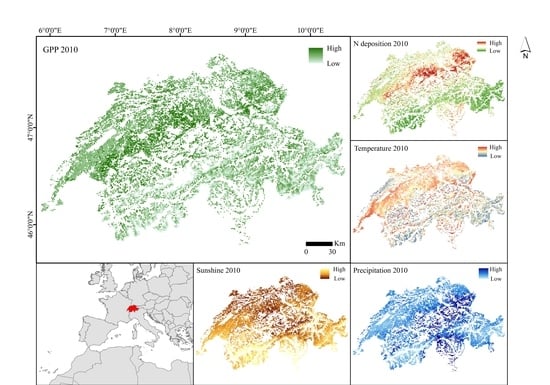
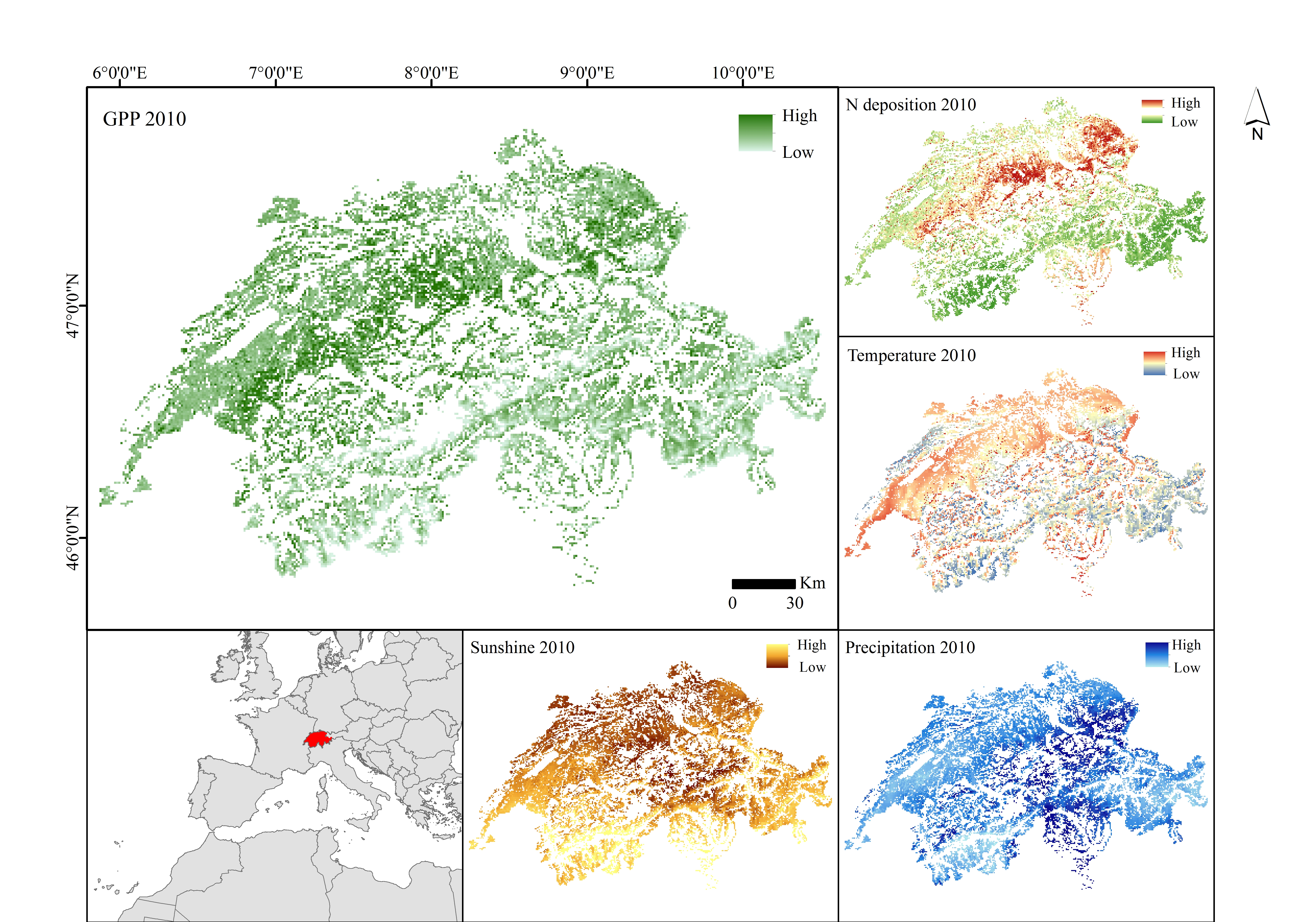
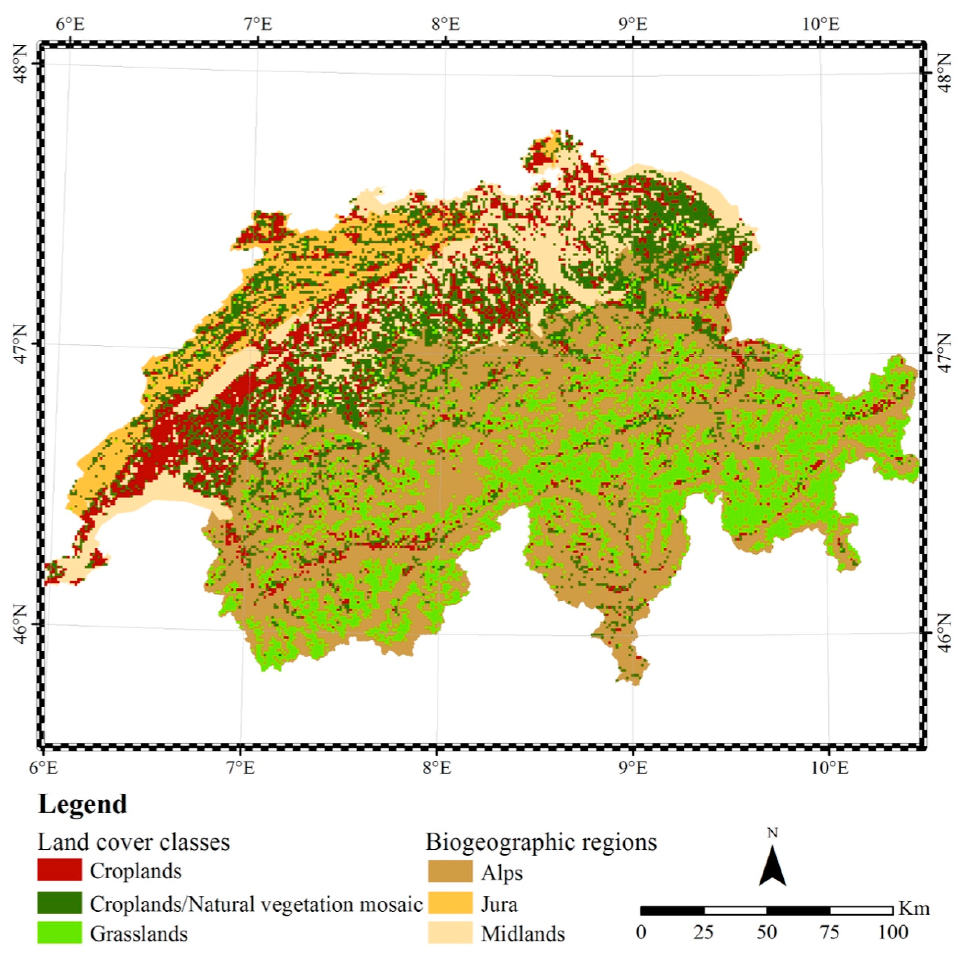
2.1. Study Area

Switzerland is divided into biogeographic regions according to flora and fauna patterns [39], (Figure 1). The Midlands are intensively managed with agricultural land use, covering ca. 50% of the area [40]. This is a heterogeneous floristic region with an altitudinal range between 256 m and 960 m a.s.l. [41]. The land cover class croplands mainly cover the Midlands (Figure 1). The altitudinal gradient impacts climatic patterns and management practices. High intensity of use occurs at altitudes lower than 1000 m a.s.l., and extensive management practices are frequent above this elevation [42,43]. In the Alps, pastures co-exist with extensively managed meadows with low yields and high plant species diversity [44,45]. The land cover class grasslands are mostly located in this area (Figure 1). Silvopastoral systems (mosaic of open grasslands, closed forest, and woody pastures) are characteristic of the Jura mountains, with diverse management practices adapted to local conditions, such as cattle stocking and logging [46,47,48]. The land cover class croplands/natural vegetation mosaic mostly covers this region (Figure 1).

The Alps divide the country producing cooler temperatures in the North than in the South, which is influenced by the Mediterranean Sea. The Atlantic Ocean also influences the Swiss climate, producing an average precipitation of ca. 2000 mm/year in the Alps and 1000–1500 mm/year in the lowlands. Altitude influences temperature, which ranges from 1°C in winter to 17°C in summer at low altitudes (<1000 m a.s.l.); from −5°C in winter to 11°C in summer at 1500 m a.s.l.; and annual means of −7.5°C at altitudes above 3000 m a.s.l. [49]. The Midlands receive more relative sunshine than the Alps and the Jura [50].

2.2. Data

2.2.1. MODIS Datasets

MODIS GPP datasets were available from the year 2000 to present (data: http://files.ntsg.umt.edu/data/NTSG_Products/). Total annual values per pixel of 8-day GPP composite products (MOD17A2 version 5.5) for the years 2000, 2007, and 2010 were used in this study [51]. These years were selected to allow a comparison with the available N deposition datasets at the time of the study. Flagged data were filtered out.

The MOD17A2 algorithm estimates GPP based on a radiation conversion efficiency approach with attenuation scalars for low temperature and water stress across biomes, using the MODIS land cover product (MOD12) (1). These parameters are specific for each biome and are available through a biome-property-look-up-table [52]. Scalars are estimated from coarse spatial resolution climate datasets. While the use of daily climate data at higher spatial resolutions can improve the quantification of GPP [53], MODIS products are still useful for characterizing how climate influences annual GPP response at regional scales [54,55]. We considered MODIS GPP as a good compromise between observational data available at a spatial resolution of 1km and data quality:

$$GPP= {\epsilon }_{max}\ast TMI{N}_{scalar}\ast VP{D}_{scalar}\ast SWRad\ast 0.45\ast FPAR$$

(1)

where ${\epsilon }_{max}$ is the maximum light use efficiency (kg C MJ⁻¹), $TMI{N}_{scalar}$ and $VP{D}_{scalar}$ are scalars between 0 and 1 that attenuate light use efficiency values based on daily minimum temperature, the vapour pressure deficit, SWrad * 0.45, corresponds to the amount of incident shortwave radiation for photosynthesis, and is the fraction of absorbed photosynthetic active radiation (PAR).

The land cover classes used in this study were obtained from the MODIS product MCD12Q1 [35], which is also used as an input to the algorithm that retrieves GPP. Therefore, we stratified the analysis, according to MODIS land cover classes, for consistency. We selected: Grasslands, croplands, and croplands/natural vegetation mosaic. The land cover classes croplands and croplands/natural vegetation mosaic are mostly found in the Midlands (or Swiss Plateau) and the Jura mountains, and the class grasslands is mainly located in the Alps. According to the Digital Height Model [56], the land cover classes selected can be found from a minimum altitude of ca. 200 m to a maximum altitude of 2634 m a.s.l. in croplands, 3033 m a.s.l. in croplands/natural vegetation mosaic, and 3570 m a.s.l. in grasslands.

The GPP algorithm is based on the UMD classification scheme proposed by the University of Maryland (UMD). However, we used the International Geosphere and Biosphere Programme (IGBP) legend, in which the UMD class croplands is divided in two classes: Croplands and croplands/natural vegetation mosaic. Friedl, et al. [35] reported an overall accuracy of 74.8% for the MCD12Q1 product using the IGBP legend with 16 classes. The classes 10, 12, and 14 were selected i.e., grasslands, croplands, and croplands/natural vegetation mosaic, respectively. All datasets were used at a spatial resolution of 1 km.

2.2.2. N Deposition Datasets

N deposition raster data for the years 2000, 2007, and 2010 [57] were produced with a spatial resolution of 1 km (Appendix A, Figure A1). The N deposition model assimilates land use information from the Swiss Land-Use Statistics point grid, which provides information based on the visual interpretation of aerial photographs at 0.1 km spatial resolution [58]. In order to provide the reader with some background about the Swiss Land-Use Statistics, we include here some details about how the selected MODIS classes relate to this dataset. The Swiss Land-Use Statistics classes considered in the model are arable land (class 221, nomenclature NOLU04), semi-natural grasslands (class 222), alpine meadows (class 241), and alpine pastures (class 242). The class arable land overlapped the MODIS classes croplands by 40.6%, the croplands/natural vegetation mosaic by 35.4%, and the grasslands by 1.35%. The class semi-natural grasslands overlapped the MODIS classes croplands/natural vegetation mosaic by 43.3%, the croplands by 11.7%, and the grasslands by 8.8%. The class alpine meadows overlapped the MODIS classes grasslands by 27.2%, the croplands/natural vegetation mosaic by 12.5%, and the croplands by 9.84%. Finally, the class alpine pastures overlapped the MODIS classes grasslands by 39.9%, the croplands/natural vegetation mosaic by 9.7%, and the croplands by 5.1%. Therefore, arable land and semi-natural grasslands are mostly covered by the MCD12Q1 classes croplands and croplands/natural vegetation mosaic, respectively, and alpine meadows and pastures are mainly covered by the MCD12Q1 class grasslands. In order to avoid possible mismatches between dry deposition and MODIS land cover classes, specific N deposition maps, including only low vegetation (excluding forests), were produced.

N deposition maps have been retrieved following a modelling approach based on wet and dry deposition of nitrate and ammonium, as well as gaseous deposition of NH₃, nitrogen dioxide (NO₂), and nitric acid. Atmospheric N deposition was mapped using a pragmatic approach that combines emission inventories, statistical dispersion models, monitoring data, spatial interpolation methods, and inferential deposition models [59]. Concentrations of the primary gaseous pollutants (NH₃ and NO₂) are estimated by means of emission maps and statistical dispersion models with a resolution of 100 × 100 m². As a result, the high spatial variability of these pollutants near emission sources can be reflected in the models. The concentrations of secondary pollutants (aerosols, HNO₃), as well as the concentrations of N in precipitation, are derived from field monitoring data by applying geo-statistical interpolation methods. Combustion processes and agricultural activities are the main sources of these atmospheric components. In particular, agricultural management practices account for 92% of ammonia (NH₃) emissions, livestock being the main contributing source. Application and storage of manure (38% and 13.8%, respectively), housing (28.4%), and grazing (2.2%) add up to 82.4% [59]. Therefore, fertilization practices influence NH₃ concentrations directly_. Modelled ammonia concentrations were validated with measured concentrations from 48 monitoring sites, R² = 0.526 (Root Mean Square Error, RMSE = 43%) [59]. Furthermore, the authors of a recent study concluded that N deposition maps provide reliable estimates for large areas [60]. (Data: https://www.bafu.admin.ch/bafu/en/home/topics/air/state/data/historical-data/maps-of-annual-values/map-of-nitrogen-deposition.html).

2.2.3. Weather Datasets

We used gridded datasets of mean annual values of temperature, yearly-accumulated precipitation, and yearly relative sunshine duration (the ratio between the effective sunshine duration and the maximal possible sunshine duration) for the years 2000, 2007, and 2010 (further information regarding the spatial variability of these datasets can be found in the Appendix A: Figure A2, Figure A3, and Figure A4) with a spatial resolution of 2.3 km [61].

Weather datasets were resampled to 1 km, allowing comparison with the other datasets. Mean annual temperature reveals standard errors of 0.5° for the Swiss Plateau/Jura and 0.7° for the Alps [62]. Cross-validation of annual precipitation datasets reports +/–20% for the Jura and the Swiss Plateau and +/−25–30% for the Alps [63]. Sunshine datasets reached median absolute values of less than 5% for the autumn/winter months and 3% for the summer months [64]. (Data: http://www.meteoswiss.admin.ch/home/climate/swiss-climate-in-detail/monthly-and-annual-maps.html?query=Grid-Data+products).

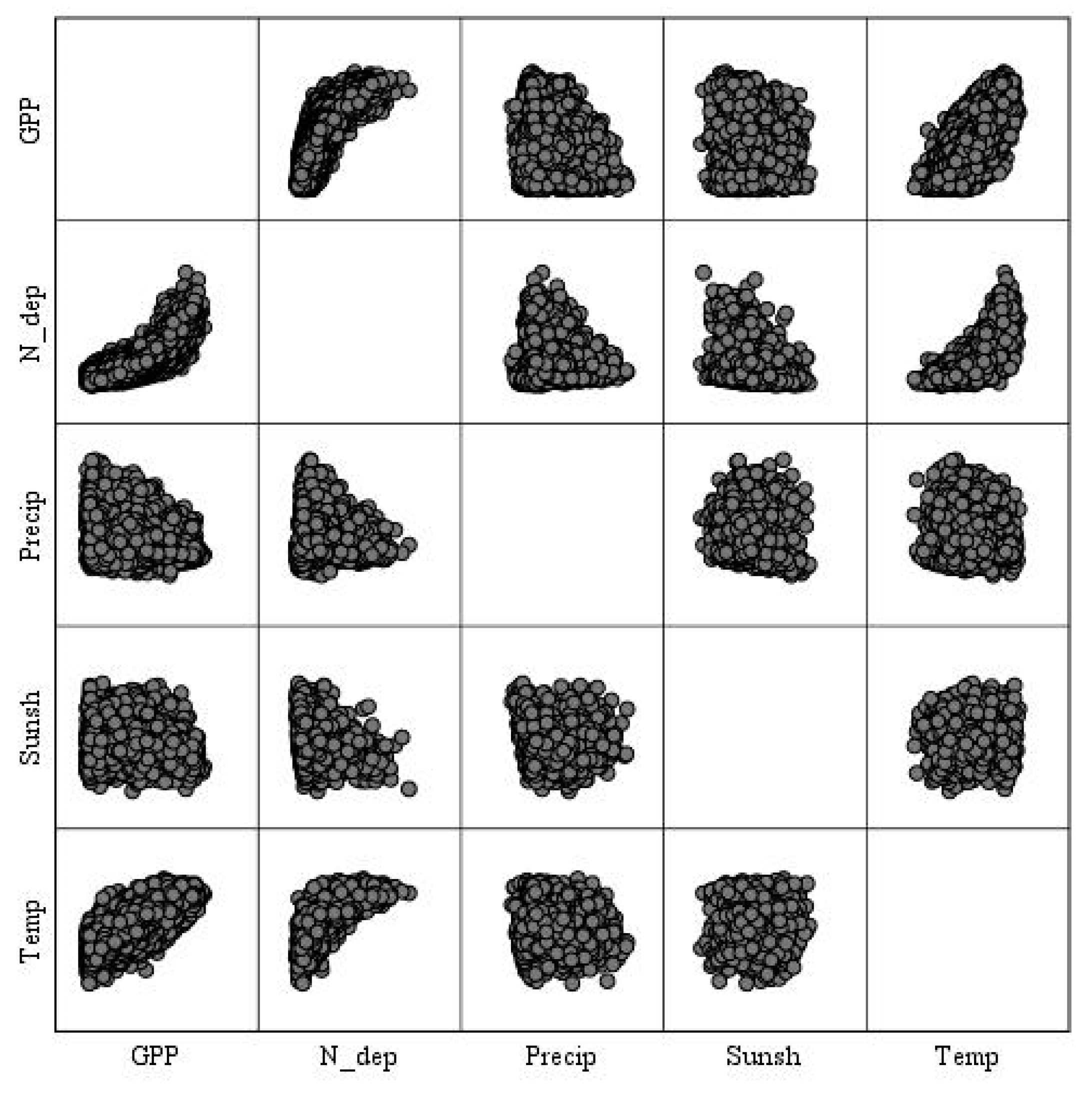
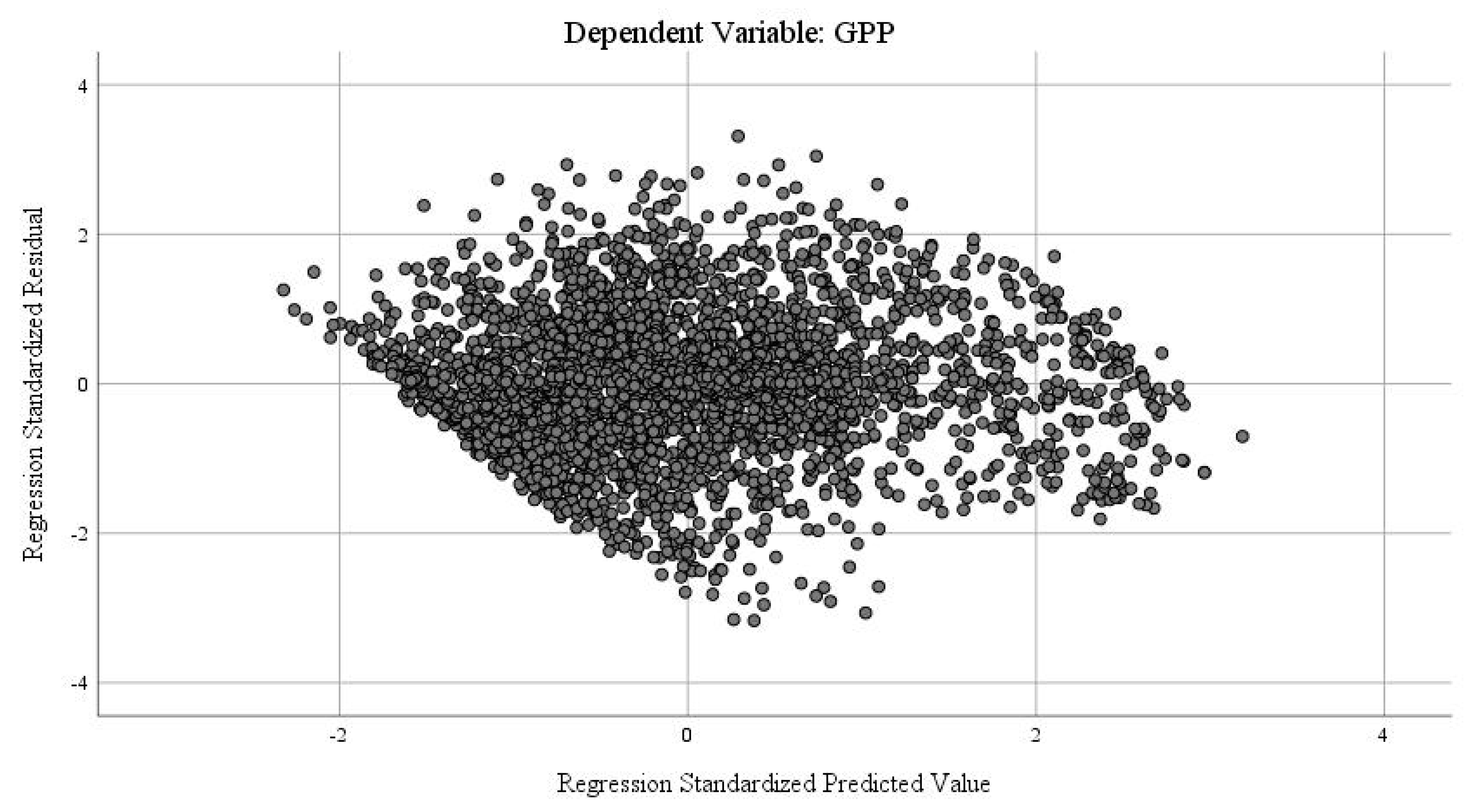
2.3. GPP Response to Limiting Factors Per Land Cover Class: Statistical Analysis

Multiple linear regression models were built for the years 2000, 2007, and 2010, according to the spatial extension of grasslands, croplands, and croplands/natural vegetation mosaic. A sample with unique values was selected in order to avoid potential oversampling caused by downscaling weather datasets to 1 km spatial resolution (see Section 2.2.3). The number of samples per land cover class was between 2066 and 3370 (

Table 1. Number of samples (n) of all the variables (gross primary production (GPP), Nitrogen (N) deposition, temperature, precipitation, and sunshine). Class 10: Grasslands, Class 12: Croplands, and Class 14: Croplands/natural vegetation mosaic.

Year	2000			2007			2010
Class	10	12	14	10	12	14	10	12	14
n	2988	2066	3327	2978	2074	3370	2965	2074	3346

). Cook’s distance [65] (4/n, n: Number of samples) helped exclude outliers and values producing leverage. GPP was the dependent variable and precipitation; temperature, sunshine, and N deposition were the independent variables for all the years. Linearity between dependent and independent variables was checked for each land cover class and year using descriptive statistics (e.g., correlation matrices Figure A5 and Figure A7) and scatterplots of the standardized residuals and standardized predicted values (Figure A6 and Figure A8). Natural logarithms were applied to the independent variable in case of non-linearity with the dependent variable (e.g., N deposition with GPP). Including a transformed version of the predictor allows incorporate non-linear associations into the linear model [66].

The final set of explanatory variables selected by the model differed per land cover class and year, according to the following procedure: The model (forward stepwise) selected the order of entry of each variable, according to the correlation between the independent variable and the dependent variable. The independent variable with the highest correlation with the dependent variable was entered into the model first. The rest of the explanatory variables were then entered into the model automatically, according to their correlation with GPP and as long as the default tolerance threshold (0.0001) of collinearity between the explanatory variable was already in the model and the new entered one was not exceeded. Collinearity statistics were estimated to check the suitability of the final set of variables selected by the model. Collinearity represents a serious issue when tolerance (T = 1 − R²) drops below 0.1 or variance inflation factor (VIF = 1/T) is above 10 [67,68]. The probability of the model to select an explanatory variable was also defined by entry criteria with a threshold of p < 0.05 and removal criteria with a threshold of p > 0.1.

Independence of residuals was analyzed with the Durbin–Watson (D–W) test. The D–W ranges from 0 to 4, with values equaling 2, indicating no correlation. Normal distribution of the standardized residuals was checked with P-P (probability-probability) plots and histograms (data not shown). Homoscedasticity was analyzed with two tests, namely Breuch–Pagan (B–P) and Koenker (K). The latter was used in case of non-normal distribution of standardized residuals. In case the assumption of homoscedasticity was violated (e.g., see Figure A8 with an inverse butterfly heteroscedasticity), heteroscedasticity-consistent (HC) standard errors were estimated [65]. The HC4 estimator was used for all the cases because of high performance in case of high leverage or non-normal distributed errors [69]. Finally, we estimated the shrunken (SR) R² with a leave-one-out cross-validation approach for statistical inference from our regression models to the population data of the studied land cover classes in Switzerland [65]. These analyses were carried out using a macro developed for SPSS^® [65,69].

2.4. Soil Characterstics Per Land Cover Class

The digital soil suitability map for Switzerland was generated in the 1970s at a scale of 1:200’000, using spatial information regarding geology, elevation, terrain attributes, and climatic zones. This map helped interpret our results and characterize the selected land cover classes in terms of soil aptitude for croplands, stone content, and water and nutrient storage capacity (

Table 2. Classes selected of the soil suitability map divided in levels.

Class	Aptitude for Croplands	StoneContent	Water Storage Capacity	Nutrient Storage Capacity
1	Very good	Not stony	Extremely low	Extremely low
2	Good	Slightly stony	Very low	Very low
3	Medium	Stony	Low	Low
4	Limited	Very stony	Medium	Medium
5	Inappropriate	Extremely stony	Good	Good
6		Unknown	Very good	Very good
7			Unknown	Unknown

) [70]. The soil suitability map was converted to a raster layer with a spatial resolution of 1 km. This raster layer was used to estimate the zonal statistics (minority and majority values). The value of the polygon that overlapped the center of the raster cell was used to assign the value to the cell. These analyses were carried out in ArcGIS 10.4.1^®.

3. Results

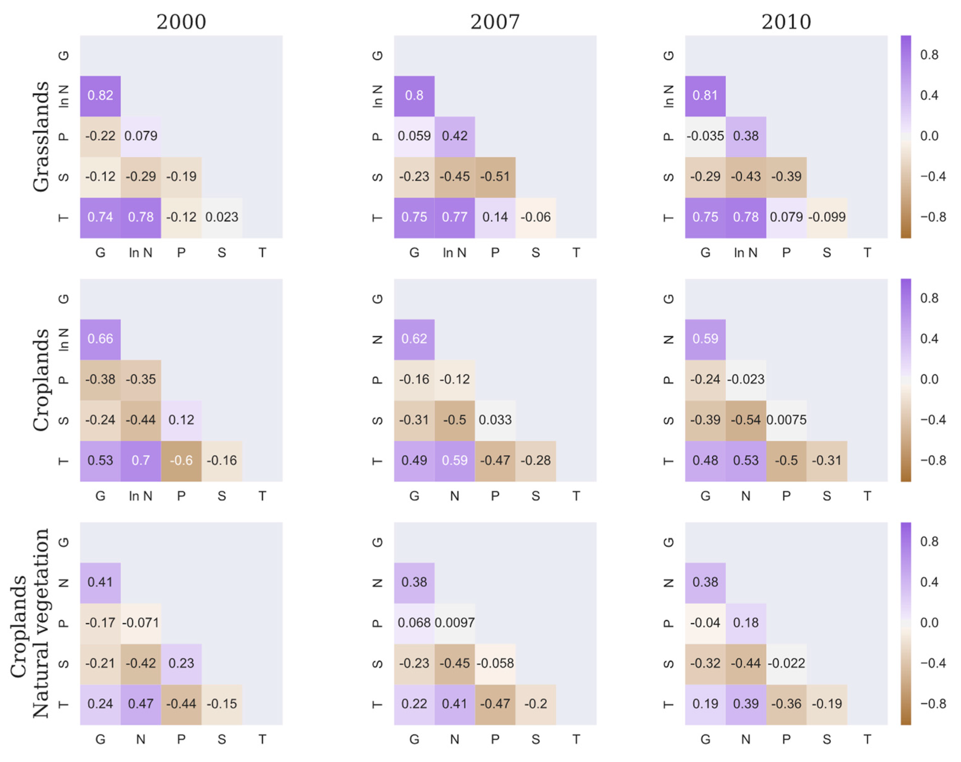
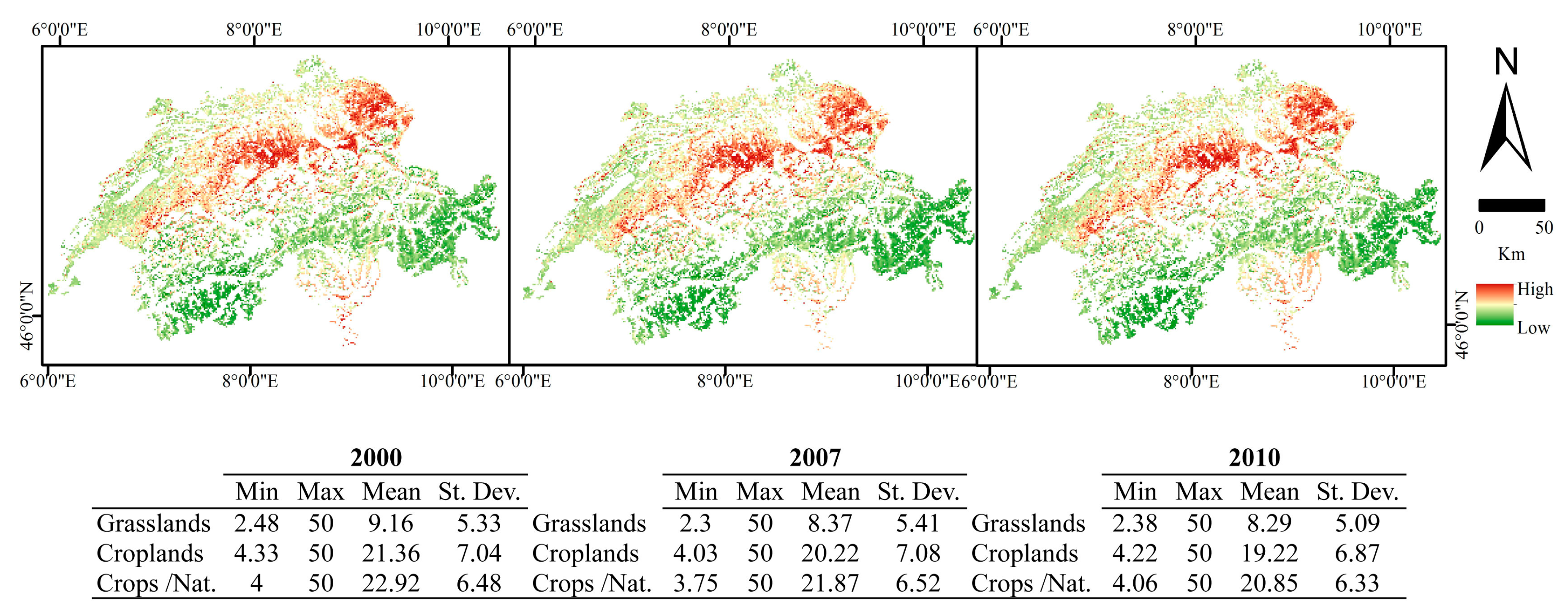
3.1. GPP Response to Limiting Factors Per Land Cover Class: Statistical Analysis

The highest correlations were found between GPP and N deposition and between GPP and temperature. The lowest correlations were found between GPP and precipitation. In particular, very low correlation or no correlation between both variables were found in 2007 and 2010 for grasslands (≈0.06 and ≈–0.04, respectively, p < 0.01) and croplands/natural vegetation mosaic (≈0.07 p < 0.01 and –0.04 p < 0.05) (Figure 2 and Appendix A,

Table A1. Pearson’s correlation between GPP: Gross primary productivity and Ln N dep: Natural logarithm of N deposition, Temp: Temperature, Precip: Precipitation, and Sunsh: Sunshine, based on a bootstrap of 1000 samples per land cover class and year. ** Statistically significant p < 0.01.

	Grasslands
	GPP 2000		GPP 2007		GPP 2010
	Pearson Correlation	95% CI	Pearson Correlation	95% CI	Pearson Correlation	95% CI
Ln N dep	0.823 ** ± 0.006	0.811— 0.833	0.798 ** ± 0.006	0.786 — 0.811	0.813 ** ± 0.006	0.801 — 0.824
Temp	0.741 ** ± 0.008	0.724 — 0.756	0.749 ** ± 0.008	0.734 — 0.763	0.748 ** ± 0.008	0.733 — 0.763
Precip	−0.220 ** ± 0.016	−0.250 — −0.190	0.059 ** ± 0.017	0.026 — 0.092	−0.035 ** ± 0.017	−0.069 — −0.001
Sunsh	−0.121 ** ± 0.019	−0.158 — −0.086	−0.233 ** ± 0.018	−0.270 — −0.197	−0.291 ** ± 0.018	−0.325 — −0.256

,

Table A2. Pearson’s correlation between GPP: Gross primary productivity and N dep: N deposition (natural logarithm used only for the year 2000), Temp: Temperature, Precip: Precipitation, and Sunsh: Sunshine, based on a bootstrap of 1000 samples per land cover class and year. ** Statistically significant p < 0.01.

	Croplands
	GPP 2000		GPP 2007		GPP 2010
	Pearson Correlation	95% CI	Pearson Correlation	95% CI	Pearson Correlation	95% CI
N dep	0.664 ** ± 0.011	0.643 — 0.687	0.615 ** ± 0.013	0.590 — 0.640	0.588 ** ± 0.013	0.560 — 0.616
Temp	0.527 ** ± 0.015	0.499 — 0.554	0.487 ** ± 0.016	0.455 — 0.518	0.477 ** ± 0.016	0.445 — 0.508
Precip	−0.383 ** ± 0.018	−0.418 — −0.347	−0.164 ** ± 0.023	−0.208 — −0.115	−0.236 ** ± 0.021	−0.276 — −0.195
Sunsh	−0.243 ** ± 0.018	−0.278 — −0.207	−0.307 ** ± 0.019	−0.346 — −0.268	−0.387 ** ± 0.016	−0.419 — −0.357

and

Table A3. Pearson’s correlation between GPP: Gross primary productivity and N dep: N deposition, Temp: Temperature, Precip: Precipitation, and Sunsh: Sunshine, based on a bootstrap of 1000 samples per land cover class and year. * Statistically significant p < 0.05 ** Statistically significant p < 0.01.

	Croplands/Natural Vegetation Mosaic
	GPP 2000		GPP 2007		GPP 2010
	Pearson Correlation	95% CI	Pearson Correlation	95% CI	Pearson Correlation	95% CI
N dep	0.411 ** ± 0.013	0.384 — 0.438	0.375 ** ± 0.014	0.349 — 0.405	0.377 ** ± 0.014	0.349 — 0.405
Temp	0.245 ** ± 0.017	0.212 — 0.277	0.220 ** ± 0.017	0.187 — 0.253	0.192 ** ± 0.017	0.160 — 0.226
Precip	−0.173 ** ± 0.016	−0.202 — −0.141	0.068 ** ± 0.016	0.037 — 0.100	−0.040 * ± 0.016	−0.074 — −0.008
Sunsh	−0.215 ** ± 0.014	−0.244 — −0.186	−0.229 ** ± 0.015	−0.259 — −0.198	−0.320 ** ± 0.014	−0.348 — −0.293

).

In grasslands, the two variables that mostly explained the GPP variance were N deposition and precipitation (

Table 3. Coefficient of determination (R²) change per variable (alphabetically ordered) that the stepwise regression model selected for grasslands, croplands, and croplands/natural vegetation mosaics. Excl: Excluded. Natural logarithms of N deposition used for grasslands in all the years and for croplands in 2000.

	Grasslands			Croplands			Croplands/Natural Vegetation Mosaics
	2000	2007	2010	2000	2007	2010	2000	2007	2010
N deposition	67.7%	63.7%	66.0%	44.1%	37.9%	34.6%	16.9%	14.1%	14.2%
Precipitation	8.1%	9.5%	13.6%	2.7%	Excl.	5.0%	2.1%	1.4%	1.0%
Sunshine	0.5%	0.1%	0.3%	0.2%	Excl.	0.7%	Excl.	0.3%	2.9%
Temperature	0.2%	1.4%	0.2%	Excl.	2.4%	0.6%	Excl.	0.5%	Excl.

). In croplands, N deposition was the independent variable that influenced the most GPP response. Precipitation followed N deposition in relevance for the years 2000 and 2010. In 2007, temperature was, however, the variable that followed N deposition in importance and the remaining variables were excluded from the model (Table 3). In croplands/natural vegetation mosaics, N deposition largely explained the GPP response followed by precipitation in the years 2000 and 2007 and sunshine in 2010 (Table 3).

In grasslands, Pearson’s correlations [65] showed that N deposition and temperature were the variables with the highest correlation with GPP (Figure 2 and Appendix A, Table A1). The model with the lowest RMSE (including all explanatory variables) reached collinearity values of 0.23 for T and 4.5 for VIF. The addition of variables to the ones already in the model (e.g., model 1: N deposition, model 2: N deposition and precipitation) increased the coefficient of determination (R²) up to 0.77 in 2000, 0.75 in 2007, and 0.8 in 2010 (

Table 4. Order of variables entered into the model and adjusted R² for grasslands, according to the addition of a new variable to the model: Ln N dep: Natural logarithm of N deposition, Temp: Temperature, Precip: Precipitation, and Sunsh: Sunshine. *** Statistically significant p < 0.001.

2000			2007			2010
Order	Adjusted R2	RMSE	Order	Adjusted R2	RMSE	Order	Adjusted R2	RMSE
Ln N dep	0.677 ***	0.225	Ln N dep	0.637 ***	0.246	Ln N dep	0.660 ***	0.220
Precip	0.759 ***	0.194	Precip	0.731 ***	0.212	Precip	0.796 ***	0.171
Sunsh	0.764 ***	0.192	Temp	0.746 ***	0.206	Temp	0.798 ***	0.170
Temp	0.766 ***	0.191	Sunsh	0.747 ***	0.206	Sunsh	0.800 ***	0.169

). In croplands, N deposition and temperature were the most correlated independent variables with GPP in all the years (Figure 2 and Appendix A, Table A2). However, correlation between these variables resulted either in exclusion of the one less correlated with GPP or a later addition into the model. The final model achieved collinearity statistics between 0.49 and 0.88 for T and between 1.14 and 2.06 for VIF. The explanatory variables reached adjusted R² values ca. 0.4 (

Table 5. Order of variables entered into the model and adjusted R² for croplands, according to the addition of a new variable to the model: N dep: N deposition, Ln N dep: Natural logarithm of N deposition, Temp: Temperature, Precip: Precipitation, and Sunsh: Sunshine. Excl: Variable excluded from the model. ** Statistically significant p < 0.01. ***Statistically significant p < 0.001.

2000			2007			2010
Order	Adjusted R2	RMSE	Order	Adjusted R2	RMSE	Order	Adjusted R2	RMSE
Ln N dep	0.441 ***	0.194	N dep	0.378 ***	0.212	N dep	0.346 ***	0.211
Precip	0.468 ***	0.190	Temp	0.402 ***	0.207	Precip	0.395 ***	0.203
Sunsh	0.470 **	0.189	Precip	Excl		Sunsh	0.402 ***	0.202
Temp	Excl		Sunsh	Excl		Temp	0.408 ***	0.201

). In croplands/natural vegetation mosaics, the explanatory variables that reached high correlation with GPP were N deposition followed by positive correlations with temperature and negative correlations with sunshine (Figure 2 and Appendix A, Table A3). The model with the lowest RMSE achieved values between 0.61 and 0.99 for T and 1 and 1.6 for VIF. Adjusted R² values reached ca. 0.18 in 2000 and 2010, and 0.16 in 2007 (

Table 6. Order of variables entered into the model and adjusted R² for croplands/natural vegetation mosaics according to the addition of a new variable to the model: N deposition: N dep, Temp: Temperature, Precip: Precipitation, and Sunsh: Sunshine. Excl: Variable excluded from the model. *** Statistically significant p < 0.001.

2000			2007			2010
Order	Adjusted R2	RMSE	Order	Adjusted R2	RMSE	Order	Adjusted R2	RMSE
N dep	0.169 ***	0.228	N dep	0.141 ***	0.247	N dep	0.142 ***	0.238
Precip	0.189 ***	0.225	Temp	0.146 ***	0.246	Sunsh	0.171 ***	0.234
Sunsh	Excl		Precip	0.160 ***	0.244	Precip	0.181 ***	0.232
Temp	Excl		Sunsh	0.163 ***	0.243	Temp	Excl

).

In grasslands, standardized residuals were normally distributed in all the cases. D–W values from 1.9 to 2 indicated independence of residuals, and the B–P test showed residuals with heteroscedasticity that were statistically significant. The leave-one-out cross-validation resulted in SR R² values ca. 0.9 for all the years. The regression coefficients to build the model for statistical inference are shown in

Table 7. Regression coefficients with heteroscedasticity-consistent standard errors for grasslands. Const: Constant, Ln N dep: Natural logarithm of N deposition, Temp: Temperature, Precip: Precipitation, and Sunsh: Sunshine. *** Statistically significant p < 0.001.

	2000		2007		2010
	Coefficients	95% CI	Coefficients	95% CI	Coefficients	95% CI
Const	−0.8075 *** ± 0.0704	−0.9456 – −0.6695	0.1089 ± 0.0971	−0.0815 – 0.2994	0.0783 – 0.0587	−0.0367 − 0.1934
Ln N dep	0.6270 *** ± 0.0121	0.6033 − 0.6507	0.5469 *** ± 0.0136	0.5201 − 0.5736	0.6095 *** ± 0.0119	0.5862 − 0.6329
Precip	−0.0002 *** ± 0.0000	—	−0.0003 *** ±0.0000	—	−0.0003 *** ± 0.0000	—
Sunsh	0.0075 *** ± 0.0013	0.0051 − 0.0100	−0.0057 *** ± 0.0016	−0.0088 – −0.0026	−0.0066 *** ± 0.0010	−0.0086 – −0.0047
Temp	0.0103 *** ± 0.0018	0.0068 ‒ 0.0139	0.0279 *** ± 0.0020	0.0240 – 0.0319	0.0123 *** ± 0.0016	0.0091 – 0.0155

. In croplands, standardized residuals were normally distributed for all the datasets. D–W values were ca. 1.9, revealing independence of errors. The B–P test showed heteroscedasticity that was statistically significant. The leave-one-out cross-validation resulted in SR R² values ca. 0.6 for all the years. The regression coefficients to create the model for statistical inference are shown in

Table 8. Regression coefficients with heteroscedasticity-consistent standard errors for croplands. Const: Constant, N dep: N deposition (natural logarithm of N deposition only used in 2000), Temp: Temperature, Precip: Precipitation, and Sunsh: Sunshine. ** Statistically significant p < 0.01. *** Statistically significant p < 0.001.

	2000		2007		2010
	Coefficients	95% CI	Coefficients	95% CI	Coefficients	95% CI
Const	-0.1581 ± 0.0783	-0.3116– -0.0046	0.5791 *** ± 0.0123	0.5549 – 0.6033	1.018 *** ± 0.0540	0.9123 – 1.124
N dep	0.4115 *** ± 0.0114	0.3891 – 0.4338	0.0197 *** ± 0.0008	0.0181 – 0.0212	0.0185 *** ± 0.0009	0.0168 – 0.0203
Precip	-0.0001 *** ± 0.0000	—	—	—	-0.0001 *** ± 0.0000	—
Sunsh	0.004** ± 0.0012	0.0017 – 0.0064	—	—	-0.0062 *** ± 0.0011	-0.0083 – -0.0042
Temp	—	—	0.0192 *** ± 0.0017	0.0158 ‒ 0.0226	0.0104 *** ± 0.0017	0.0070 – 0.0138

. In croplands/natural vegetation mosaics, standardized residuals were not normally distributed in all the samples. D–W values ca. 1.8 showed independence of errors. The K test indicated heteroscedasticity that was statistically significant. The leave-one-out cross-validation resulted in SR R² values ca. 0.4 for all the years. The regression coefficients to generate the model for statistical inference are shown in

Table 9. Regression coefficients with heteroscedasticity-consistent standard errors for croplands/natural vegetation mosaic. Const: Constant, N dep: N deposition, Temp: Temperature, Precip: Precipitation, and Sunsh: Sunshine. *** Statistically significant p < 0.001.

	2000		2007		2010
	Coefficients	95% CI	Coefficients	95% CI	Coefficients	95% CI
Const	1.077 *** ± 0.0175	1.042 – 1.111	0.9787 *** ± 0.0643	0.8527 – 1.1048	1.568 *** ± 0.0478	1.475 – 1.662
N dep	0.0167 *** ± 0.0006	0.0154 – 0.0179	0.0123 *** ± 0.0008	0.0107 – 0.0138	0.0138 *** ± 0.0007	0.0123 – 0.0152
Precip	-0.0001 *** ± 0.0000	—	0.0001 *** ± 0.0000	—	-0.0001 *** ± 0.0000	—
Sunsh	—	—	-0.0041 *** ± 0.0010	-0.0061 – -0.0021	-0.0120 *** ± 0.0010	-0.0139 – -0.0101
Temp	—	—	0.0205 *** ± 0.0022	0.0161 – 0.0248	—	—

.

3.2. Soil Characteristics Per Land Cover Class

The zonal-statistics analysis using the digital soil suitability map characterized the aptitude for croplands, stone content, and water and nutrient storage capacity of the three land cover classes. The results indicated that the land cover class grasslands were mostly located in areas inappropriate for agriculture. The majority of the values of this land cover class, with regard to stone content and water and nutrient storage capacity, resulted in the category unknown. However, the visual inspection of the digital soil suitability map for Switzerland [70] reveals that the Alps are characterized by extremely low, very low, and low water and nutrient storage capacity values. Croplands were mainly placed in areas with very good aptitude for agriculture production, slightly stony, and with good water and nutrient storage capacity. Croplands/natural vegetation mosaic were mostly characteristic of stony areas inappropriate for agriculture, with good water and nutrient storage capacity.

4. Discussion

GPP Response to Limiting Factors Per Land Cover Class: Statistical Analysis

N deposition achieved a higher predictive power of GPP response than climatic factors, especially in alpine grasslands. However, the observed non-linear relationships between N deposition and GPP in grasslands for all the years suggest plant N saturation even at the observed low N deposition rates. Grasslands are more sensitive to plant N saturation than other ecosystems, which produces non-linear primary productivity responses at lower N saturation thresholds [71]. Non-linear responses change according to climate factors and soil conditions [72].

The correlations between climatic factors and GPP shown in our study are in line with the modelling results of Beer, et al. [6] for Switzerland. In particular, we found a low correlation between precipitation and GPP. Nevertheless, this climatic factor was relevant to generate the models. Therefore, analyzing the correlation results was key to determining the role of this variable in the considered years (Figure 2 and Appendix A, Table A1, Table A2 and Table A3). We also found a positive correlation between N deposition and temperature—such a correlation was also reported by Maskell, et al. [73]. Notwithstanding temperature was a relevant factor to explain GPP variance in the years 2000, 2007, and 2010, a higher correlation between N deposition and GPP as well as the collinearity threshold produced that N deposition overshadowed the role of temperature in the models. Therefore, studying how limiting factors of GPP interact among them is key before drawing conclusions from statistical models. Moreover, the comparison of results among years shows how the magnitude of influence of those limiting factors can vary. We also reported negative correlations between sunshine and GPP. Beer, et al. [6] suggested that this negative correlation occurs because sun radiation may induce evapotranspiration, which affects water availability and limit GPP. Besides, productivity may increase with diffuse sun radiation produced by the complex topography and cloudy conditions. Baptist and Choler [74] also observed this relationship, comparing the impact of overcast and cloudless conditions on C assimilation in alpine meadows. On the other hand, growth cycles constrained by altitudinal gradients may result in lower seasonal GPP values [74]. Nevertheless, Zeeman, et al. [75] concluded that accounting for the growing season length and management period do not improve GPP estimations in grasslands managed at different elevations in Switzerland. The MODIS land cover classes considered in our study spread across a wide altitudinal range in which different growing seasons occur within the same land cover class (see Section 2.2.1). Therefore, we consider the use of annual values appropriated to carry out our analysis. In particular, grasslands have a standard growing season from February to November [76].

The predictive performance of N deposition decreased in croplands and croplands/natural vegetation mosaics. Legume-based crops (grassland in rotation) that reach high rates of N inputs through N₂ fixation can maintain a moderate-high level of productivity in the long-term [77]. Moreover, areas with high intensity of use have additional input of nutrients, and therefore modelled N deposition may play a less relevant role to predict GPP response. In addition, the class croplands/natural vegetation mosaic is widely located in the Jura mountains, which is characterized by various management practices. In particular, extensification processes that decrease biodiversity of woody pastures have occurred on remote areas of the Jura mountains, while high intensity of use practices have contributed to preserving biodiversity on the proximity of populated zones [47,78]. Therefore, the low influence of N deposition in GPP response could be explained by complex biosphere-atmosphere interactions triggered by mixed management practices and high species richness [79,80,81]. In particular, Bassin, et al. [23] showed that N deposition could enhance, diminish, or not affect the productivity of certain species in abundant plant communities. Abiotic and biotic factors mediate N deposition effects in terrestrial ecosystems, producing different impacts among biomes [82]. Consequently, different results are expected in areas with different management practices and water and nutrient storage capacity.

5. Outlook

High N input through animal manure, mineral fertilizer, and N deposition are common in croplands and can produce nutrient leaching and eutrophication of surface waters [83,84,85]. In Switzerland, N deposition is the source that provides the least amount of N inputs in agricultural soils [19]. However, critical loads (threshold below which adverse environmental effects do not occur according to present knowledge) of N deposition have been exceeded in most of the forest and semi-natural ecosystems [59]. Despite N deposition decreasing since the mid-1990s, N deposition remains still too high in many areas [60]. In particular, the highest N exceedances occur in the lowlands where intensive management practices lead to high ammonia emissions because of high manure inputs [59,86]. In our study, the predictive performance of N deposition decreased in those areas with high intensity of use. N can stimulate growth differently according to species-specific physiology and other co-limiting nutrients, such as phosphorous and potassium [23,87]. However, in those cultivated areas, growth is regulated by specific management practices. Detailed information about management practices (e.g., fertilization and irrigation), soil components, and crop types could shed light on the impact of N deposition on C fixation response in managed areas. Therefore, we recommend further research in that field. Determining nutrient balance helps characterize N dynamics and the influence of nutrient sources in managed agroecosystems [88,89].

On the other hand, N can be a driver, not only of biomass but also of ecosystem respiration in grasslands and croplands, which can turn C sinks into sources [10,90,91]. In addition, controlling factors of GPP response can have opposite effects. For example, low quantities of N deposition promote C storage while high temperatures produce C losses [24,92]. Taking into account these interactions is of utter importance because of ever more frequent extreme climatic episodes worldwide. Therefore, quantifying the impact of N deposition on the C budget together with other factors, such as land management practices and extreme climatic events, is crucial to understanding ecosystem processes. The emission-based model adopted in this study to quantify N deposition provided good estimates for large areas and produced similar results when compared with alternative methods [60]. Therefore, this approach is considered a reliable source of information for studies carried out at a national scale. In addition, we suggest the development of further lines of research, taking into account the climate inter-annual variability in the study areas, which could provide answers to the low correlation found between precipitation and GPP. Model simulations have shown the importance of coupling N and C cycles to account for vegetation dynamics and to improve global patterns of C and N fluxes [93,94]. There are still limitations on modelling sources of fixed N and land management changes, as well as coupling terrestrial C and N cycles [95,96]. Nevertheless, we expect our study to contribute to the inclusion of N deposition datasets in Earth system models to better account for N dynamics. This could improve predictions of C uptake in different ecosystems [97,98,99].

6. Conclusions

Our study emphasizes the importance of studying how limiting factors of GPP response relate among them and to GPP to derive conclusions about their explanatory performance. We showed the role of N deposition in explaining GPP variance in soils with low nutrient storage capacity and how these areas present plant N saturation. The most important climatic variable to build all the models was precipitation. Temperature and sunshine were occasionally relevant in specific years. However, temperature was the variable with the second highest correlation with GPP. Therefore, interactions among controlling factors need to be taken into account before drawing conclusions from the final set of explanatory variables selected by a model.

This study contributes to characterizing large spatial patterns of GPP in Switzerland and how controlling factors vary in areas with complex topography affected by local climatic conditions and different land management patterns. However, we recommend developing further research lines to disentangle the impact of controlling factors on GPP variance in ecosystems with high intensity of use, mixed management practices, and high species richness as well as the role of precipitation in GPP response in the study area. Finally, we foster accounting for N dynamics and land management practices in conjunction with climatic factors in C budget models to improve our understanding of complex ecosystem processes.

References

1. Lal, R. Soil Carbon Sequestration Impacts on Global Climate Change and Food Security. Science 2004, 304, 1623–1627. [Google Scholar] [CrossRef]
2. Chapin, F.S., III; Woodwell, G.M.; Randerson, J.T.; Rastetter, E.B.; Lovett, G.M.; Baldocchi, D.D.; Clark, D.A.; Harmon, M.E.; Schimel, D.S.; Valentini, R.; et al. Reconciling Carbon-Cycle Concepts, Terminology, and Methods. Ecosystems 2006, 9, 1041–1050. [Google Scholar] [CrossRef]
3. Anav, A.; Friedlingstein, P.; Beer, C.; Ciais, P.; Harper, A.; Jones, C.; Murray-Tortarolo, G.; Papale, D.; Parazoo, N.C.; Peylin, P.; et al. Spatiotemporal patterns of terrestrial gross primary production: A review. Rev. Geophys. 2015, 53, 785–818. [Google Scholar] [CrossRef] [Green Version]
4. Monfreda, C.; Ramankutty, N.; Foley, J.A. Farming the planet: 2. Geographic distribution of crop areas, yields, physiological types, and net primary production in the year 2000. Glob. Biogeochem. Cycles 2008, 22. [Google Scholar] [CrossRef] [Green Version]
5. Zhang, Y.; Yu, G.; Yang, J.; Wimberly, M.C.; Zhang, X.; Tao, J.; Jiang, Y.; Zhu, J. Climate-driven global changes in carbon use efficiency. Glob. Ecol. Biogeogr. 2014, 23, 144–155. [Google Scholar] [CrossRef]
6. Beer, C.; Reichstein, M.; Tomelleri, E.; Ciais, P.; Jung, M.; Carvalhais, N.; Rödenbeck, C.; Arain, M.A.; Baldocchi, D.; Bonan, G.B.; et al. Terrestrial gross carbon dioxide uptake: Global distribution and covariation with climate. Science 2010, 329, 834–838. [Google Scholar] [CrossRef] [PubMed]
7. Liu, D.; Li, Y.; Wang, T.; Peylin, P.; MacBean, N.; Ciais, P.; Jia, G.; Ma, M.; Ma, Y.; Shen, M.; et al. Contrasting responses of grassland water and carbon exchanges to climate change between Tibetan Plateau and Inner Mongolia. Agric. For. Meteorol. 2018, 249, 163–175. [Google Scholar] [CrossRef]
8. Verstraeten, W.W.; Veroustraete, F.; Feyen, J. On temperature and water limitation of net ecosystem productivity: Implementation in the C-Fix model. Ecol. Model. 2006, 199, 4–22. [Google Scholar] [CrossRef]
9. Stevens, C.J.; Lind, E.M.; Hautier, Y.; Harpole, W.S.; Borer, E.T.; Hobbie, S.; Seabloom, E.W.; Ladwig, L.; Bakker, J.D.; Chu, C.; et al. Anthropogenic nitrogen deposition predicts local grassland primary production worldwide. Ecology 2015, 96, 1459–1465. [Google Scholar] [CrossRef] [Green Version]
10. Volk, M.; Obrist, D.; Novak, K.; Giger, R.; Bassin, S.; Fuhrer, J. Subalpine grassland carbon dioxide fluxes indicate substantial carbon losses under increased nitrogen deposition, but not at elevated ozone concentration. Glob. Chang. Biol. 2011, 17, 366–376. [Google Scholar] [CrossRef]
11. De Vries, W.; Posch, M.; Simpson, D.; Reinds, G.J. Modelling long-term impacts of changes in climate, nitrogen deposition and ozone exposure on carbon sequestration of European forest ecosystems. Sci. Total Environ. 2017, 605–606, 1097–1116. [Google Scholar] [CrossRef] [PubMed]
12. Sun, Z.; Wang, X.; Yamamoto, H.; Tani, H.; Zhong, G.; Yin, S.; Guo, E. Spatial pattern of GPP variations in terrestrial ecosystems and its drivers: Climatic factors, CO2 concentration and land-cover change, 1982–2015. Ecol. Inform. 2018, 46, 156–165. [Google Scholar] [CrossRef]
13. Freibauer, A.; Rounsevell, M.D.A.; Smith, P.; Verhagen, J. Carbon sequestration in the agricultural soils of Europe. Geoderma 2004, 122, 1–23. [Google Scholar] [CrossRef]
14. Smith, P. Carbon sequestration in croplands: The potential in Europe and the global context. Eur. J. Agron. 2004, 20, 229–236. [Google Scholar] [CrossRef]
15. Lal, R. Soil carbon sequestration to mitigate climate change. Geoderma 2004, 123, 1–22. [Google Scholar] [CrossRef]
16. LeBauer, D.S.; Treseder, K.K. Nitrogen limitation of net primary productivity in terrestrial ecosystems is globally distributed. Ecology 2008, 89, 371–379. [Google Scholar] [CrossRef] [PubMed]
17. Sala, O.E.; Stuart Chapin, F., III; Armesto, J.J.; Berlow, E.; Bloomfield, J.; Dirzo, R.; Huber-Sanwald, E.; Huenneke, L.F.; Jackson, R.B.; Kinzig, A.; et al. Global Biodiversity Scenarios for the Year 2100. Science 2000, 287, 1770–1774. [Google Scholar] [CrossRef]
18. Oehri, J.; Schmid, B.; Schaepman-Strub, G.; Niklaus, P.A. Biodiversity promotes primary productivity and growing season lengthening at the landscape scale. Proc. Natl. Acad. Sci. USA 2017, 114, 10160–10165. [Google Scholar] [CrossRef] [Green Version]
19. FSO, Agriculture and Forestry. Swiss Agriculture. Pocket Statistics. Federal Statistics Office; Federal Department of Home Affairs: Neuchâtel, Switzerland, 2015; p. 36. Available online: https://www.bfs.admin.ch/bfs/en/home/statistics/agriculture-forestry.assetdetail.349914.html (accessed on 29 May 2017).
20. FOAG. Swiss Agricultural Policy; Swiss Federal Office for Agriculture: Liebefeld, Switzerland, 2004; p. 16. Available online: https://www.cbd.int/financial/pes/swiss-pesagriculturalpolicy.pdf (accessed on 10 October 2016).
21. Hitz, C.; Egli, M.; Fitze, P. Below-ground and above-ground production of vegetational organic matter along a climosequence in alpine grasslands. J. Plant Nutr. Soil Sci. 2001, 164, 389–397. [Google Scholar] [CrossRef]
22. Leifeld, J.; Zimmermann, M.; Fuhrer, J.; Conen, F. Storage and turnover of carbon in grassland soils along an elevation gradient in the Swiss Alps. Glob. Chang. Biol. 2009, 15, 668–679. [Google Scholar] [CrossRef]
23. Bassin, S.; Volk, M.; Suter, M.; Buchmann, N.; Fuhrer, J. Nitrogen deposition but not ozone affects productivity and community composition of subalpine grassland after 3 yr of treatment. New Phytol. 2007, 175, 523–534. [Google Scholar] [CrossRef] [Green Version]
24. Bala, G.; Devaraju, N.; Chaturvedi, R.K.; Caldeira, K.; Nemani, R. Nitrogen deposition: How important is it for global terrestrial carbon uptake. Biogeosciences 2013, 10, 7147–7160. [Google Scholar] [CrossRef]
25. Zaehle, S. Terrestrial nitrogen-carbon cycle interactions at the global scale. Philos. Trans. R. Soc. B Biol. Sci. 2013, 368. [Google Scholar] [CrossRef] [PubMed]
26. Stocker, B.D.; Prentice, I.C.; Cornell, S.E.; Davies-Barnard, T.; Finzi, A.C.; Franklin, O.; Janssens, I.; Larmola, T.; Manzoni, S.; Näsholm, T.; et al. Terrestrial nitrogen cycling in Earth system models revisited. New Phytol. 2016, 210, 1165–1168. [Google Scholar] [CrossRef] [Green Version]
27. Chang, J.; Ciais, P.; Viovy, N.; Vuichard, N.; Herrero, M.; Havlík, P.; Wang, X.; Sultan, B.; Soussana, J.-F. Effect of climate change, CO2 trends, nitrogen addition, and land-cover and management intensity changes on the carbon balance of European grasslands. Glob. Chang. Biol. 2016, 22, 338–350. [Google Scholar] [CrossRef]
28. Running, S.W.; Nemani, R.R.; Heinsch, F.A.; Zhao, M.; Reeves, M.; Hashimoto, H. A continuous satellite-derived measure of global terrestrial primary production. BioScience 2004, 54, 547–560. [Google Scholar] [CrossRef]
29. Turner, D.P.; Ritts, W.D.; Cohen, W.B.; Gower, S.T.; Running, S.W.; Zhao, M.; Costa, M.H.; Kirschbaum, A.A.; Ham, J.M.; Saleska, S.R.; et al. Evaluation of MODIS NPP and GPP products across multiple biomes. Remote Sens. Environ. 2006, 102, 282–292. [Google Scholar] [CrossRef]
30. Turner, D.P.; Ritts, W.D.; Cohen, W.B.; Gower, S.T.; Zhao, M.; Running, S.W.; Wofsy, S.C.; Urbanski, S.; Dunn, A.L.; Munger, J.W. Scaling Gross Primary Production (GPP) over boreal and deciduous forest landscapes in support of MODIS GPP product validation. Remote Sens. Environ. 2003, 88, 256–270. [Google Scholar] [CrossRef] [Green Version]
31. Zhao, M.; Heinsch, F.A.; Nemani, R.R.; Running, S.W. Improvements of the MODIS terrestrial gross and net primary production global data set. Remote Sens. Environ. 2005, 95, 164–176. [Google Scholar] [CrossRef]
32. Zhao, M.; Running, S.W.; Nemani, R.R. Sensitivity of Moderate Resolution Imaging Spectroradiometer (MODIS) terrestrial primary production to the accuracy of meteorological reanalyses. J. Geophys. Res. Biogeosci. 2006, 111. [Google Scholar] [CrossRef] [Green Version]
33. Turner, D.P.; Ritts, W.D.; Cohen, W.B.; Maeirsperger, T.K.; Gower, S.T.; Kirschbaum, A.A.; Running, S.W.; Zhao, M.; Wofsy, S.C.; Dunn, A.L.; et al. Site-level evaluation of satellite-based global terrestrial gross primary production and net primary production monitoring. Glob. Chang. Biol. 2005, 11, 666–684. [Google Scholar] [CrossRef]
34. Heinsch, F.A.; Zhao, M.; Running, S.W.; Kimball, J.S.; Nemani, R.R.; Davis, K.J.; Bolstad, P.V.; Cook, B.D.; Desai, A.R.; Ricciuto, D.M.; et al. Evaluation of remote sensing based terrestrial productivity from MODIS using regional tower eddy flux network observations. IEEE Trans. Geosci. Remote Sens. 2006, 44, 1908–1923. [Google Scholar] [CrossRef]
35. Friedl, M.A.; Sulla-Menashe, D.; Tan, B.; Schneider, A.; Ramankutty, N.; Sibley, A.; Huang, X. MODIS Collection 5 global land cover: Algorithm refinements and characterization of new datasets. Remote Sens. Environ. 2010, 114, 168–182. [Google Scholar] [CrossRef]
36. Chen, Z.; Yu, G.; Zhu, X.; Wang, Q.; Niu, S.; Hu, Z. Covariation between gross primary production and ecosystem respiration across space and the underlying mechanisms: A global synthesis. Agric. For. Meteorol. 2015, 203, 180–190. [Google Scholar] [CrossRef] [Green Version]
37. Solberg, S.; Dobbertin, M.; Reinds, G.J.; Lange, H.; Andreassen, K.; Fernandez, P.G.; Hildingsson, A.; de Vries, W. Analyses of the impact of changes in atmospheric deposition and climate on forest growth in European monitoring plots: A stand growth approach. For. Ecol. Manag. 2009, 258, 1735–1750. [Google Scholar] [CrossRef]
38. Cerasoli, S.; Campagnolo, M.; Faria, J.; Nogueira, C.; Da Conceição Caldeira, M. On estimating the gross primary productivity of Mediterranean grasslands under different fertilization regimes using vegetation indices and hyperspectral reflectance. Biogeosciences 2018, 15, 5455–5471. [Google Scholar] [CrossRef]
39. FOEN. Biogeographic regions of Switzerland (CH); Federal Office for the Environment Federal Office for Environment/Species, Ecosystems, Landscapes Division (FOEN): Ittigen, Switzerland, 2004; Available online: https://map.geo.admin.ch/?lang=en&topic=bafu&X=190000.00&Y=660000.00&zoom=1&bgLayer=ch.swisstopo.pixelkarte-farbe&catalogNodes=766,767,784,798,804,806,768,781,1361 (accessed on 8 March 2017).
40. FSO. Land Use in Switzerland. Results of the Swiss Land Use Statistics; FSO: Neuchâtel, Switzerland, 2013; p. 24. Available online: https://www.bfs.admin.ch/bfs/en/home/statistics/territory-environment.assetdetail.348992.html (accessed on March 2018).
41. Gonseth, Y.; Wohlgemuth, T.; Sansonnens, B.; Buttler, A. Les Régions Biogéographiques de la Suisse—Explications et Division Standard; Cahier de l’environnement n° 137. Office fédéral de l’environnement, des forêts et du paysage; OFEFP: Berne, Switzerland, 2001; p. 48. [Google Scholar]
42. Bolliger, J.; Hagedorn, F.; Leifeld, J.; Böhl, J.; Zimmermann, S.; Soliva, R.; Kienast, F. Effects of land-use change on carbon stocks in Switzerland. Ecosystems 2008, 11, 895–907. [Google Scholar] [CrossRef]
43. Leifeld, J.; Bassin, S.; Fuhrer, J. Carbon stocks in Swiss agricultural soils predicted by land-use, soil characteristics, and altitude. Agric. Ecosyst. Environ. 2005, 105, 255–266. [Google Scholar] [CrossRef]
44. Kampmann, D.; Herzog, F.; Jeanneret, P.; Konold, W.; Peter, M.; Walter, T.; Wildi, O.; Lüscher, A. Mountain grassland biodiversity: Impact of site conditions versus management type. J. Nat. Conserv. 2008, 16, 12–25. [Google Scholar] [CrossRef]
45. Graf, R.; Müller, M.; Korner, P.; Jenny, M.; Jenni, L. 20% loss of unimproved farmland in 22 years in the Engadin, Swiss Alps. Agric. Ecosyst. Environ. 2014, 185, 48–58. [Google Scholar] [CrossRef]
46. Peringer, A.; Siehoff, S.; Chételat, J.; Spiegelberger, T.; Buttler, A.; Gillet, F. Past and future landscape dynamics in pasture-woodlands of the Swiss Jura Mountains under climate change. Ecol. Soc. 2013, 18, 11. [Google Scholar] [CrossRef]
47. Chételat, J.; Kalbermatten, M.; Lannas, K.S.M.; Spiegelberger, T.; Wettstein, J.-B.; Gillet, F.; Peringer, A.; Buttler, A. A Contextual Analysis of Land-Use and Vegetation Changes in Two Wooded Pastures in the Swiss Jura Mountains. Ecol. Soc. 2013, 18, 39. [Google Scholar] [CrossRef]
48. Gavazov, K.S.; Peringer, A.; Buttler, A.; Gillet, F.; Spiegelberger, T. Dynamics of forage production in pasture-woodlands of the Swiss Jura mountains under projected climate change scenarios. Ecol. Soc. 2013, 18. [Google Scholar] [CrossRef]
49. Meteoswiss, Climate of Switzerland. 2014. Available online: http://www.meteoswiss.admin.ch/home/climate/the-climate-of-switzerland.html (accessed on 8 March 2017).
50. Meteoswiss, Climate Change in Switzerland. 2015. Available online: http://www.meteoswiss.admin.ch/content/dam/meteoswiss/de/Ungebundene-Seiten/Publikationen/doc/mch_klimawandel_63-13_high.pdf (accessed on 26 March 2018).
51. Running, S.W.; Zhao, M. Gross Primary Productivity 8-Day L4 Global 1Km (MOD17A2), v 5.0 and 5.5 NASA EOSDIS Land Processes DAAC; USGS Earth Resources Observation and Science (EROS) Center: Sioux Falls, South Dakota, 2000. Available online: https://lpdaac.usgs.gov (accessed on 16 January 2017).
52. Running, S.W.; Zhao, M. User’s Guide Daily GPP and Annual NPP (MOD17A2/A3) Products NASA Earth Observing System MODIS Land Algorithm; NASA MODIS Land Team: Greenbelt, MD, USA.
53. Kooistra, L.; Bergsma, A.; Chuma, B.; de Bruin, S. Development of a dynamic web mapping service for vegetation productivity using earth observation and in situ sensors in a sensor web based approach. Sensors 2009, 9, 2371–2388. [Google Scholar] [CrossRef]
54. Weiskittel, A.R.; Crookston, N.L.; Radtke, P.J. Linking climate, gross primary productivity, and site index across forests of the western United States. Can. J. For. Res. 2011, 41, 1710–1721. [Google Scholar] [CrossRef]
55. Zhang, Y.; Song, C.; Zhang, K.; Cheng, X.; Zhang, Q. Spatial-temporal variability of terrestrial vegetation productivity in the Yangtze River Basin during 2000–2009. J. Plant Ecol. 2014, 7, 10–23. [Google Scholar] [CrossRef]
56. Swisstopo. Digital Height Model, SwissALTI3D; Federal Office of Topography: Köniz, Switzerland, 2015; Available online: https://shop.swisstopo.admin.ch/de/products/height_models/alti3D (accessed on 25 May 2017).
57. FOEN. Nitrogen Deposition. Meteotest and Federal Office of the Environment; Federal Office for the Environment (FOEN): Ittigen, Switzerland, 2016; Available online: https://www.bafu.admin.ch/bafu/en/home/topics/air/state/data/historical-data/maps-of-annual-values/map-of-nitrogen-deposition.html (accessed on 2 March 2017).
58. FSO. Swiss Land-Use Statistics, ha-grid (Arealstatistik Schweiz); Federal Statistical Office: Neuchâtel, Switzerland, 2005; Available online: https://www.bfs.admin.ch/bfs/de/home/statistiken/raum-umwelt/erhebungen/area.html (accessed on 5 May 2017).
59. Rihm, B.; Achermann, B. Critical Loads of Nitrogen and Their Exceedances; Swiss Contribution to the Effects-Oriented Work under the Convention on Long-Range Transboundary Air Pollution (UNECE); Federal Office for the Environment: Ittigen, Switzerland, 2016; p. 78. Available online: https://www.bafu.admin.ch/bafu/en/home/topics/air/publications-studies/publications/Critical-Loads-of-Nitrogen-and-their-Exceedances.html (accessed on 26 May 2017).
60. Thimonier, A.; Kosonen, Z.; Braun, S.; Rihm, B.; Schleppi, P.; Schmitt, M.; Seitler, E.; Waldner, P.; Thöni, L. Total deposition of nitrogen in Swiss forests: Comparison of assessment methods and evaluation of changes over two decades. Atmos. Environ. 2019, 198, 335–350. [Google Scholar] [CrossRef]
61. Meteoswiss. MeteoSwiss Grid-Data Products; Meteoswiss: Zurich-Airport, Switzerland, 2013; Available online: http://www.meteoswiss.admin.ch/home/climate/swiss-climate-in-detail/monthly-and-annual-maps.html?query=Grid-Data+products (accessed on 26 March 2018).
62. Meteoswiss. Monthly and Yearly Mean Temperature: TabsM and TabsY; Meteoswiss: Zurich-Airport, Switzerland, 2016; Available online: http://www.meteoswiss.admin.ch/content/dam/meteoswiss/de/service-und-publikationen/produkt/raeumliche-daten-temperatur/doc/ProdDoc_TabsM.pdf (accessed on 26 March 2018).
63. Meteoswiss. Monthly and Yearly Precipitation: RhiresM and RhiresY; Meteoswiss: Zurich-Airport, Switzerland, 2016; Available online: http://www.meteoswiss.admin.ch/content/dam/meteoswiss/de/service-und-publikationen/produkt/raeumliche-daten-niederschlag/doc/ProdDoc_RhiresM.pdf (accessed on 26 March 2018).
64. Meteoswiss. Monthly and Yearly Relative Sunshine Duration: SreIM and SrelY; Meteoswiss: Zurich-Airport, Switzerland, 2016; Available online: http://www.meteoswiss.admin.ch/content/dam/meteoswiss/de/service-und-publikationen/produkt/raeumliche-daten-sonnenschein/doc/ProdDoc_SrelM.pdf (accessed on 26 March 2018).
65. Darlington, R.B.; Hayes, A.F. Regression Analysis and Linear Models: Concepts, Applications, and Implementation; Guilford Publications: New York, NY, USA, 2016. [Google Scholar]
66. James, G.; Witten, D.; Hastie, T.; Tibshirani, R. Linear Regression. In An Introduction to Statistical Learning: With Applications in R; Springer New York: New York, NY, USA, 2013; pp. 59–126. [Google Scholar]
67. Midi, H.; Sarkar, S.K.; Rana, S. Collinearity diagnostics of binary logistic regression model. J. Interdiscip. Math. 2010, 13, 253–267. [Google Scholar] [CrossRef] [Green Version]
68. Dormann, C.F.; Elith, J.; Bacher, S.; Buchmann, C.; Carl, G.; Carré, G.; Marquéz, J.R.G.; Gruber, B.; Lafourcade, B.; Leitão, P.J.; et al. Collinearity: A review of methods to deal with it and a simulation study evaluating their performance. Ecography 2013, 36, 27–46. [Google Scholar] [CrossRef]
69. Hayes, A.F.; Cai, L. Using heteroskedasticity-consistent standard error estimators in OLS regression: An introduction and software implementation. Behav. Res. Methods 2007, 39, 709–722. [Google Scholar] [CrossRef] [PubMed] [Green Version]
70. FOAG. Digital Soil Suitability Map of Switzerland; Federal Office for Agriculture (FOAG): Liebefeld, Switzerland, 1980; Available online: https://www.blw.admin.ch/blw/de/home/politik/datenmanagement/geografisches-informationssystem-gis/download-geodaten.html (accessed on 1 February 2017).
71. Tian, D.; Wang, H.; Sun, J.; Niu, S. Global evidence on nitrogen saturation of terrestrial ecosystem net primary productivity. Environ. Res. Lett. 2016, 11. [Google Scholar] [CrossRef]
72. Ye, J.S.; Pei, J.Y.; Fang, C. Under which climate and soil conditions the plant productivity–precipitation relationship is linear or nonlinear? Sci. Total Environ. 2018, 616–617, 1174–1180. [Google Scholar] [CrossRef]
73. Maskell, L.C.; Smart, S.M.; Bullock, J.M.; Thompson, K.; Stevens, C.J. Nitrogen deposition causes widespread loss of species richness in British habitats. Glob. Chang. Biol. 2010, 16, 671–679. [Google Scholar] [CrossRef]
74. Baptist, F.; Choler, P. A simulation of the importance of length of growing season and canopy functional properties on the seasonal gross primary production of temperate alpine meadows. Ann. Bot. 2008, 101, 549–559. [Google Scholar] [CrossRef] [PubMed]
75. Zeeman, M.J.; Hiller, R.; Gilgen, A.K.; Michna, P.; Plüss, P.; Buchmann, N.; Eugster, W. Management and climate impacts on net CO2 fluxes and carbon budgets of three grasslands along an elevational gradient in Switzerland. Agric. For. Meteorol. 2010, 150, 519–530. [Google Scholar] [CrossRef]
76. Gómez Giménez, M.; de Jong, R.; Della Peruta, R.; Keller, A.; Schaepman, M.E. Determination of grassland use intensity based on multi-temporal remote sensing data and ecological indicators. Remote Sens. Environ. 2017, 198, 126–139. [Google Scholar] [CrossRef]
77. Ledgard, S.F. Nitrogen cycling in low input legume-based agriculture, with emphasis on legume/grass pastures. Plant Soil 2001, 228, 43–59. [Google Scholar] [CrossRef]
78. Huber, R.; Rigling, A.; Bebi, P.; Brand, F.S.; Briner, S.; Buttler, A.; Elkin, C.; Gillet, F.; Grêt-Regamey, A.; Hirschi, C.; et al. Sustainable land use in mountain regions under global change: Synthesis across scales and disciplines. Ecol. Soc. 2013, 18. [Google Scholar] [CrossRef]
79. Schuster, M.J.; Smith, N.G.; Dukes, J.S. Responses of aboveground C and N pools to rainfall variability and nitrogen deposition are mediated by seasonal precipitation and plant community dynamics. Biogeochemistry 2016, 129, 389–400. [Google Scholar] [CrossRef]
80. Bassin, S.; Volk, M.; Fuhrer, J. Species Composition of Subalpine Grassland is Sensitive to Nitrogen Deposition, but Not to Ozone, After Seven Years of Treatment. Ecosystems 2013, 16, 1105–1117. [Google Scholar] [CrossRef]
81. Vankoughnett, M.R.; Henry, H.A.L. Soil freezing and N deposition: Transient vs multi-year effects on plant productivity and relative species abundance. New Phytol. 2014, 202, 1277–1285. [Google Scholar] [CrossRef] [PubMed]
82. Matson, P.; Lohse, K.A.; Hall, S.J. The globalization of nitrogen deposition: Consequences for terrestrial ecosystems. Ambio 2002, 31, 113–119. [Google Scholar] [CrossRef] [PubMed]
83. Krupa, S.V. Effects of atmospheric ammonia (NH3) on terrestrial vegetation: A review. Environ. Pollut. 2003, 124, 179–221. [Google Scholar] [CrossRef]
84. Bergström, A.K.; Jansson, M. Atmospheric nitrogen deposition has caused nitrogen enrichment and eutrophication of lakes in the northern hemisphere. Glob. Chang. Biol. 2006, 12, 635–643. [Google Scholar] [CrossRef]
85. Camargo, J.A.; Alonso, Á. Ecological and toxicological effects of inorganic nitrogen pollution in aquatic ecosystems: A global assessment. Environ. Int. 2006, 32, 831–849. [Google Scholar] [CrossRef] [PubMed]
86. Hesterberg, R.; Blatter, A.; Fahrni, M.; Rosset, M.; Neftel, A.; Eugster, W.; Wanner, H. Deposition of nitrogen-containing compounds to an extensively managed grassland in central Switzerland. Environ. Pollut. 1996, 91, 21–34. [Google Scholar] [CrossRef]
87. Bassin, S.; Schalajda, J.; Vogel, A.; Suter, M. Different types of sub-alpine grassland respond similarly to elevated nitrogen deposition in terms of productivity and sedge abundance. J. Veg. Sci. 2012, 23, 1024–1034. [Google Scholar] [CrossRef]
88. Della Peruta, R.; Keller, A. A regional modelling tool to assess the risk of accumulation of nutrients, trace metals and pesticides in agricultural soils (iMSoil). BGS-Bulletin 37: 9–15. Annèe internationale des Sols—et Maintenant? Pédologie, S.S.D., Ed.; Genève, Switzerland, 2016. Available online: http://www.soil.ch/cms/publikationen/bulletins/bulletin-37/ (accessed on 2 June 2017).
89. Gómez Giménez, M.; Della Peruta, R.; de Jong, R.; Keller, A.; Schaepman, M.E. Spatial Differentiation of Arable Land and Permanent Grassland to Improve a Land Management Model for Nutrient Balancing. IEEE J. Sel. Top. Appl. Earth Obs. Remote Sens. 2016, 9, 5655–5665. [Google Scholar] [CrossRef]
90. Migliavacca, M.; Reichstein, M.; Richardson, A.D.; Colombo, R.; Sutton, M.A.; Lasslop, G.; Tomelleri, E.; Wohlfahrt, G.; Carvalhais, N.; Cescatti, A.; et al. Semiempirical modeling of abiotic and biotic factors controlling ecosystem respiration across eddy covariance sites. Glob. Chang. Biol. 2011, 17, 390–409. [Google Scholar] [CrossRef]
91. Volk, M.; Enderle, J.; Bassin, S. Subalpine grassland carbon balance during 7 years of increased atmospheric N deposition. Biogeosciences 2016, 13, 3807–3817. [Google Scholar] [CrossRef] [Green Version]
92. Zscheischler, J.; Reichstein, M.; Harmeling, S.; Rammig, A.; Tomelleri, E.; Mahecha, M.D. Extreme events in gross primary production: A characterization across continents. Biogeosciences 2014, 11, 2909–2924. [Google Scholar] [CrossRef]
93. Zaehle, S.; Friend, A.D.; Friedlingstein, P.; Dentener, F.; Peylin, P.; Schulz, M. Carbon and nitrogen cycle dynamics in the O-CN land surface model: 2. Role of the nitrogen cycle in the historical terrestrial carbon balance. Glob. Biogeochem. Cycles 2010, 24. [Google Scholar] [CrossRef] [Green Version]
94. Smith, B.; Wärlind, D.; Arneth, A.; Hickler, T.; Leadley, P.; Siltberg, J.; Zaehle, S. Implications of incorporating N cycling and N limitations on primary production in an individual-based dynamic vegetation model. Biogeosciences 2014, 11, 2027–2054. [Google Scholar] [CrossRef] [Green Version]
95. Xu, R.; Prentice, I.C. Modelling the demand for new nitrogen fixation by terrestrial ecosystems. Biogeosciences 2017, 14, 2003–2017. [Google Scholar]
96. Churkina, G.; Zaehle, S.; Hughes, J.; Viovy, N.; Chen, Y.; Jung, M.; Heumann, B.W.; Ramankutty, N.; Heimann, M.; Jones, C. Interactions between nitrogen deposition, land cover conversion, and climate change determine the contemporary carbon balance of Europe. Biogeosciences 2010, 7, 2749–2764. [Google Scholar] [CrossRef]
97. Drewniak, B.; Gonzalez-Meler, M.A. Earth system model needs for including the interactive representation of nitrogen deposition and drought effects on forested ecosystems. Forests 2017, 8, 267. [Google Scholar] [CrossRef]
98. Cai, X.; Yang, Z.L.; Fisher, J.B.; Zhang, X.; Barlage, M.; Chen, F. Integration of nitrogen dynamics into the Noah-MP land surface model v1.1 for climate and environmental predictions. Geosci. Model Dev. 2016, 9, 1–15. [Google Scholar] [CrossRef] [Green Version]
99. McGuire, A.D.; Sitch, S.; Clein, J.S.; Dargaville, R.; Esser, G.; Foley, J.; Heimann, M.; Joos, F.; Kaplan, J.; Kicklighter, D.W.; et al. Carbon balance of the terrestrial biosphere in the twentieth century: Analyses of CO2, climate and land use effects with four process-based ecosytem models. Glob. Biogeochem. Cycles 2001, 15, 183–206. [Google Scholar] [CrossRef]
Figure 1. Study area. Land cover classes distributed across (aggregated, e.g., Alps) biogeographic regions. Coordinate system: WGS84.
Remotesensing 11 01135 g001
Figure 2. Correlation matrix between the dependent and independent variables per year and land cover class (p < 0.01 mostly, see Appendix A, Table A1, Table A2 and Table A3). G: GPP, N: N deposition, ln N: natural logarithm of N deposition, P: Precipitation, S: Sunshine, and T: Temperature.
Remotesensing 11 01135 g002