Floating Xylene Spill Segmentation from Ultraviolet Images via Target Enhancement
by
Shuyue Zhan
1, 
Chao Wang
1,
Shuchang Liu
2,
Kaibo Xia
1,
Hui Huang
1,*,
Xiaorun Li
3,*,
Caicai Liu
4 and
Ren Xu
4 1
Ocean College, Zhejiang University, Zhoushan, Zhejiang 316021, China
2
College of Science, Zhejiang University of Technology, Hangzhou, Zhejiang 310014, China
3
Institute of Advanced Technology, Zhejiang University, Hangzhou, Zhejiang 310007, China
4
East China Sea Environmental Monitoring Center, Shanghai, Ministry of Natural Resources of the People’s Rrepublic of China, Beijing 310058, China
*
Authors to whom correspondence should be addressed.
Remote Sens. 2019, 11(9), 1142; https://0-doi-org.brum.beds.ac.uk/10.3390/rs11091142
Submission received: 4 March 2019
/
Revised: 1 May 2019
/
Accepted: 7 May 2019
/
Published: 13 May 2019
Abstract
:Automatic colorless floating hazardous and noxious substances (HNS) spill segmentation is an emerging research topic. Xylene is one of the priority HNSs since it poses a high risk of being involved in an HNS incident. This paper presents a novel algorithm for the target enhancement of xylene spills and their segmentation in ultraviolet (UV) images. To improve the contrast between targets and backgrounds (waves, sun reflections, and shadows), we developed a global background suppression (GBS) method to remove the irrelevant objects from the background, which is followed by an adaptive target enhancement (ATE) method to enhance the target. Based on the histogram information of the processed image, we designed an automatic algorithm to calculate the optimal number of clusters, which is usually manually determined in traditional cluster segmentation methods. In addition, necessary pre-segmentation processing and post-segmentation processing were adopted in order to improve the performance. Experimental results on our UV image datasets demonstrated that the proposed method can achieve good segmentation results for chemical spills from different backgrounds, especially for images with strong waves, uneven intensities, and low contrast.

1. Introduction
With the worldwide demand for chemicals increasing sharply, the amount of chemicals transported by sea has increased by 3.5 times in the past 20 years because of sea transport’s low costs for carrying large quantities over long distances [1]. The majority of these chemicals are categorized as hazardous and noxious substances (HNSs), which are defined as any substance other than oil that, if introduced into the marine environment, is likely to create human health hazards, harm living resources and other marine life, damage amenities, and/or interfere with other legitimate uses of the sea [2]. With the increase in the marine transportation of HNSs among major ports, the risk of HNS spillages is further increased [3]. HNS spills have their own characteristics that are different from oil spills, especially considering the wide variety of products that may be involved [4]. Approaches for oil detection may not be suitable for HNS spill detection. In order to deal with a spill accident, accurate and rapid knowledge of the spill area, location, and movement enables one to develop effective and efficient countermeasures and therefore significantly reduce the ecological impacts and costs of cleanup operations [5]. Manual segmentation of spills from a large number of images is time-consuming and laborious. Therefore, automatically detecting those spill regions becomes an important issue.
Unlike other target segmentation tasks, chemical spills have their own challenges. First, in the list of the top 10 chemicals that are likely to pose the highest risk of being involved in an HNS incident [6], eight chemicals are colorless in the visible spectrum, meaning that the difference in the color between the leaked area and the water surface is small and difficult to identify. Second, most liquid chemicals have low viscosities and low surface tension forces, which lead to a thin liquid film on the water surface [7] and invalidate the detection method using the changes in surface roughness, such as synthetic aperture radar (SAR) [8]. Third, due to container ports being frequent accident occurrence places due to their complex environment, accident images usually record the spill target and background, including surface waves, sun reflections, and the shadows caused by buildings, ships, equipment, and clouds. All these challenges make it difficult to recognize chemical leakage targets from the background. To overcome these problems, several relative studies have focused on sensors and automatic detection methods.
With respect to sensors, an HNS monitoring with radar remote sensing experimental study showed that some chemicals are undetectable using SAR images [8]. This seems to be caused by the high volatility of the tested products and the relatively long time lag between the discharge and observations. Compared to the use of SAR images, optical images allow for a wide swath monitoring and relatively low costs, thereby providing more frequent information [9,10]. It is the optical characteristic and chemical properties of oil that makes it possible to detect oil spills using optical sensors [9,11]. Some chemical products in HNSs, especially hydrocarbon chemicals, have similar chemistries (OH, CN, and CH bonds) with oil, thereby indicating that there is the potential to use optical images to detect these spills. In the area of oil spill detection, ultraviolet (UV) sensors have been proven to be able to detect thin layers (<0.1 μm) [12], thereby indicating its potential for detecting thin chemical layers. Recently, unmanned aerial vehicles (UAVs) are becoming popular in coastal environmental monitoring, such as litter, pollution, beach erosion, land use, and anthropological impacts [13,14,15,16], because of their flexibility and low cost. UAVs equipped with UV sensors have a great potential for the real-time detection of floating HNSs.
Compared to choosing detection hardware, automatic target segmentation is a more challenging task in image understanding and computer vision due to the variety, low contrast, and uneven illumination of chemical spill images. Many methods of image segmentation have been proposed to detect targets on water surfaces, including thresholding [17], level sets [18], active contour models [19], the Mean-Shift [20], and neural networks [21]. The level sets method is a branch of active contour model, which represents contour as the zero level set of a higher dimensional function. The use of this method can provide more flexibility in the implementation of active contours. The main drawbacks are high dependence on initializations and it is time-consuming [22]. The active contour model is based on an energy minimization scheme. The Chan–Vese model is one of the most representative region-based one, which converts image segmentation into a problem of finding contours. With the homogeneity assumption in an image, this method usually fails to segment image with inhomogeneous intensities [23], while the images of HNS usually present inhomogeneity. The Mean-Shift is a nonparametric iterative algorithm, which has been used in image segmentation. It builds upon the concept of kernel density estimation (KDE), which may misclassify target pixels into its neighborhood background because of low contrast, which is also common in HNS images. The other disadvantage is its time-consuming nature [24]. Neural network is an efficient supervised learning method. To obtain a good performance neural network, its parameters should be adjusted by a long time back-propagation training process within a large number of training images. It is also highly sensitive to initial training parameter settings [25]. Dependence on initialization may affect the generalization and efficiency of segmentation method.
Among these algorithms, thresholding is one of the most popular methods that is used for image segmentation because of its effectiveness and simplicity, and it can assist to make an initial estimation for some complex segmentation methods [26]. Thresholding methods can be classified into three practical categories:
(2) adapting an adaptive local threshold, such as fuzzy c-means [29] and adaptive thresholding [30]; and
(3) considering the spatial local information for classifying the pixels, such as two-dimensional (2D) Otsu, 2D maximum entropy [31], and spatial fuzzy c-means [32].
Category 1 only searches for a global threshold from the gray value information and uses it to divide the image into two regions. This method is susceptible to complex backgrounds, low signal-to-noise ratios (SNRs), and uneven illumination, leading to many segmentation errors. Categories 2 and 3 set the threshold according to local explicit and implicit variants, thereby enhancing the recognition accuracy of pixels. However, all these methods fail in the case of images with low contrast between the target and background, which is common in chemical spill images. To fill this gap in chemical spill detection, we conducted a colorless chemical spill experiment to verify the difference and distinguish between a transparent chemical spill and a clean water surface in UV images. These images were captured simulating the moving of UAV. Based on the characteristics of chemical spill images, an automatic chemical spill segmentation method is proposed in this literature. In our method, we first conduct pre-segmentation processing to smooth the noise while maintaining the target’s sharpness. Second, we propose global background suppression (GBS) to reduce the complexity of the background and adaptive target enhancement to improve the saliency of the target. After the above steps, a local fuzzy thresholding method (LFTM), which is robust in resisting artifacts and noise as that proposed in [33], is adopted to separate the target and the other regions, and the number of regions in the processed image is determined using histogram analysis. The new method can resist complex backgrounds and is suitable for the detection of weak targets. In our experiment of floating xylene on water, the proposed method achieves promising performance on UV image. The next work is to apply our algorithm on UV images that are captured on UAV.
The rest of this paper is arranged as follows. In Section 2, the overall proposed methodology is outlined. In Section 3, we conduct an experiment to obtain colorless xylene spill images and implement our method as described. Performance of the algorithm is discussed. Finally, in Section 4, conclusions on the method and suggestions to future work are mentioned.
2. Method
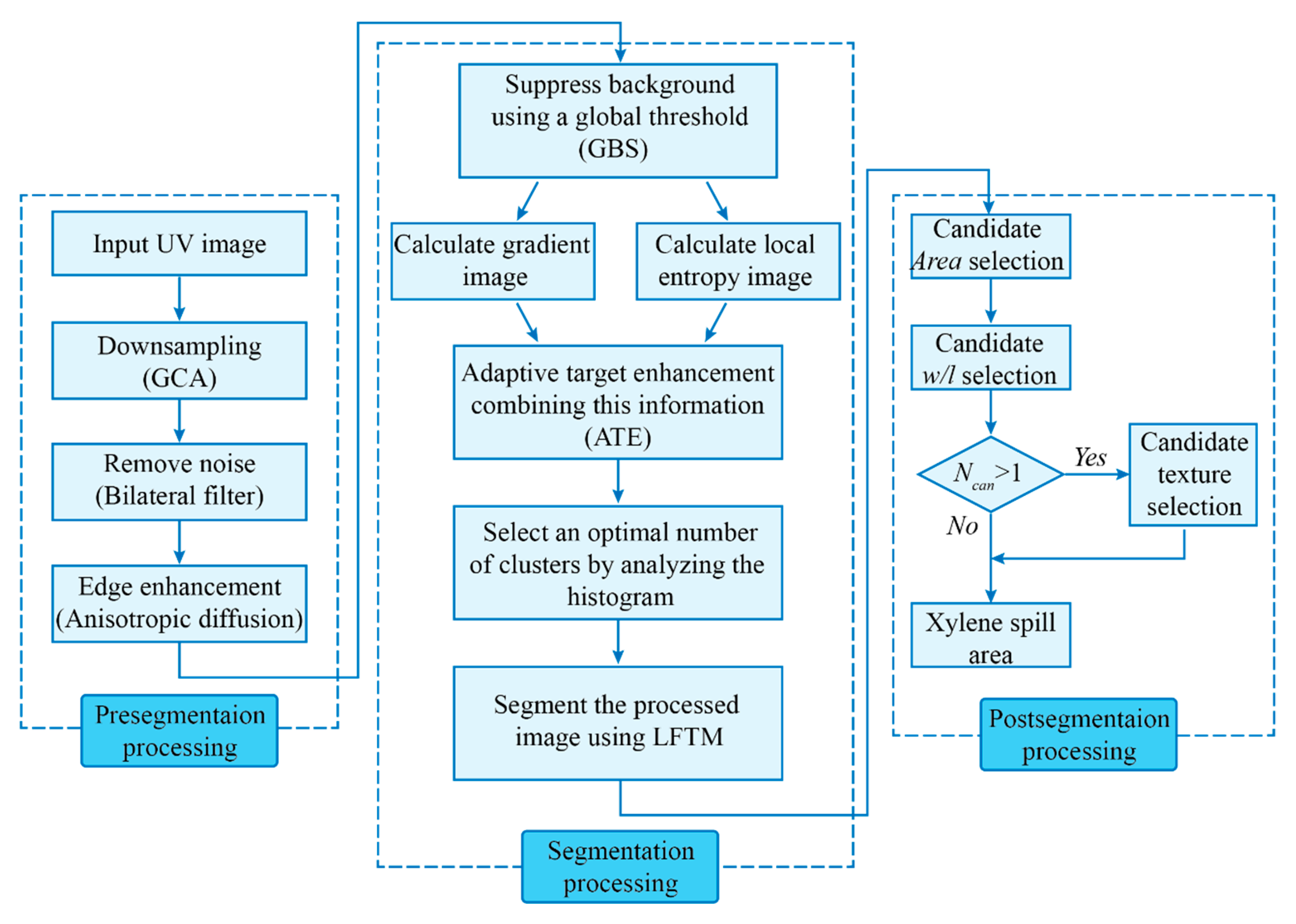
The main contribution of our work is to propose a method for distinguishing the spill areas of transparent liquid chemicals floating on water. In this section, we introduce all the processing steps of our method. The UV images are processed using the workflow illustrated in Figure 1.
2.1. Pre-Segmentation Processing
2.1.1. Downsampling
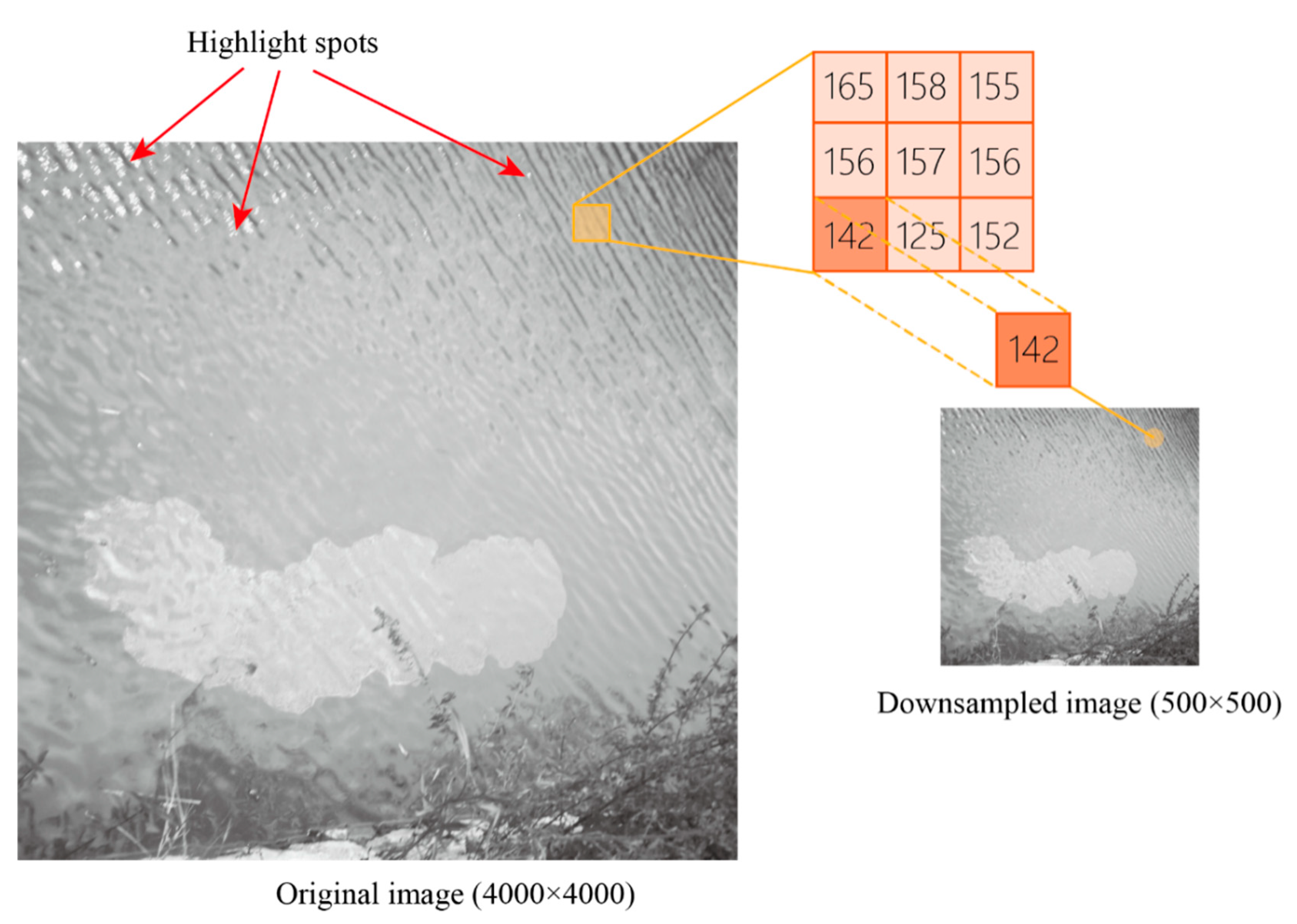
The original image has a resolution of 4000 × 4000. It is time-consuming to directly process these images. As shown in Figure 2, the spill target is generally brighter than the surrounding background, while some small bright speckles, such as leaves and solar reflections, also are bright, thereby causing the spill target to be incorrectly identified. To improve the processing efficiency and eliminate the effects of small bright speckles at the local scale, a simple but effective downsampling method, which is called grid cell analysis (GCA) [34], was adopted. This step is not necessary if there is an advanced hardware system and lower real-time requirements. The GCA algorithm first divides an image into m × n grids. Then, it calculates the minimum intensity value of each cell, and finally it downsamples the original image by replacing each cell with the corresponding minimum intensity value. Through the GCA process, the spill region features are preserved, while most of the small speckle noise is removed. The image resolution is reduced, thereby leading to an efficient calculation for further processing.
Figure 2 shows the calculation operation of the GCA. The left image is the original image and the right is the downsampled one. Comparing the two images, it is obvious that some highlighted spots that are indicated by the red arrows in left picture are removed. In this work, we select 8 × 8 blocks, which means that the downsampled image’s resolution is 500 × 500.
2.1.2. Noise Removal
After the GCA process, several impulse noises may randomly occur in the image, which may influence the sensitivity of the lateral adaptive target enhancement (ATE) process in which the image gradient value is a key component. Meanwhile, an edge-preserving filter is required in order to remove the image noise without over blurring the edges of the spill. A bilateral filter is a nonlinear, edge-preserving, and noise-reducing smoothing filter that meets the above requirements [35]. The new intensity value of each pixel is calculated using a weighted average of the original intensity values from nearby pixels. These weights follow a Gaussian distribution. Compared to other common filters, the bilateral filter can achieve a promising denoising result [36].
2.1.3. Edge Enhancement
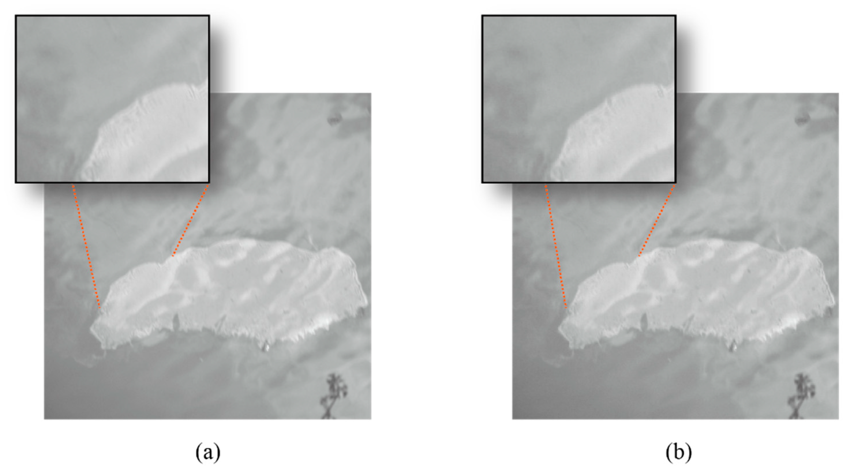
To compensate for the information loss caused by the smoothing operation, we choose the anisotropic diffusion algorithm to enhance the saliency of the spill region’s boundaries and suppress the weak edges and small structures inside the background [37]. Figure 3 demonstrates the effect of the pre-segmentation processing. With the help of the GCA, bilateral filter and anisotropic diffusion operation, the image noise and small unwanted objects are discarded, and the target boundaries are enhanced.
2.2. Image Segmentation Algorithm
2.2.1. Global Background Suppression
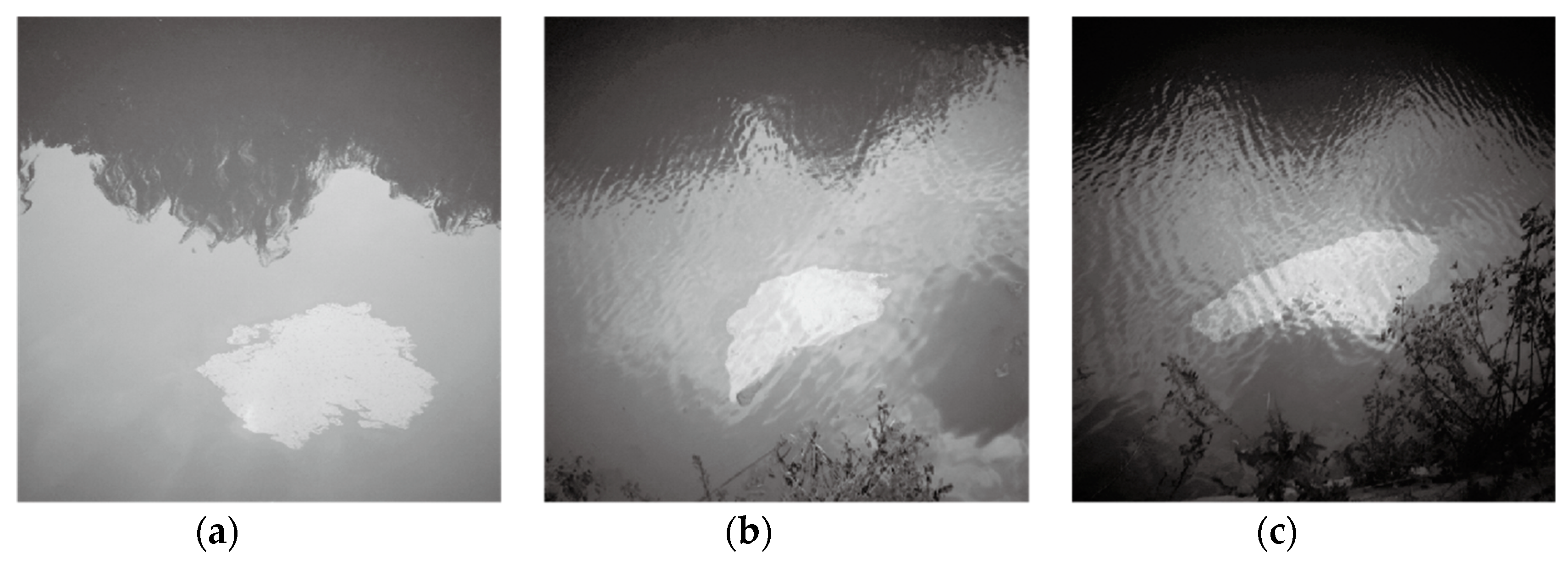
As shown in the UV images in Figure 4, we can conclude three important properties that help us to achieve the segmentation goal. First, the pixel intensities of the target are higher than its nearby pixel intensities, thereby causing a detectable edge around the target. Second, the pixel intensities of the background have a wide range because of the existence of shadows, waves, and sun reflections. Therefore, it is impossible to use gray value information to distinguish between the target and the background. Third, there are different intensity distributions among the different UV images due to the viewing angle, water surface conditions, and varying illuminations, which increase the difficulty of modeling the distributions of the UV images.
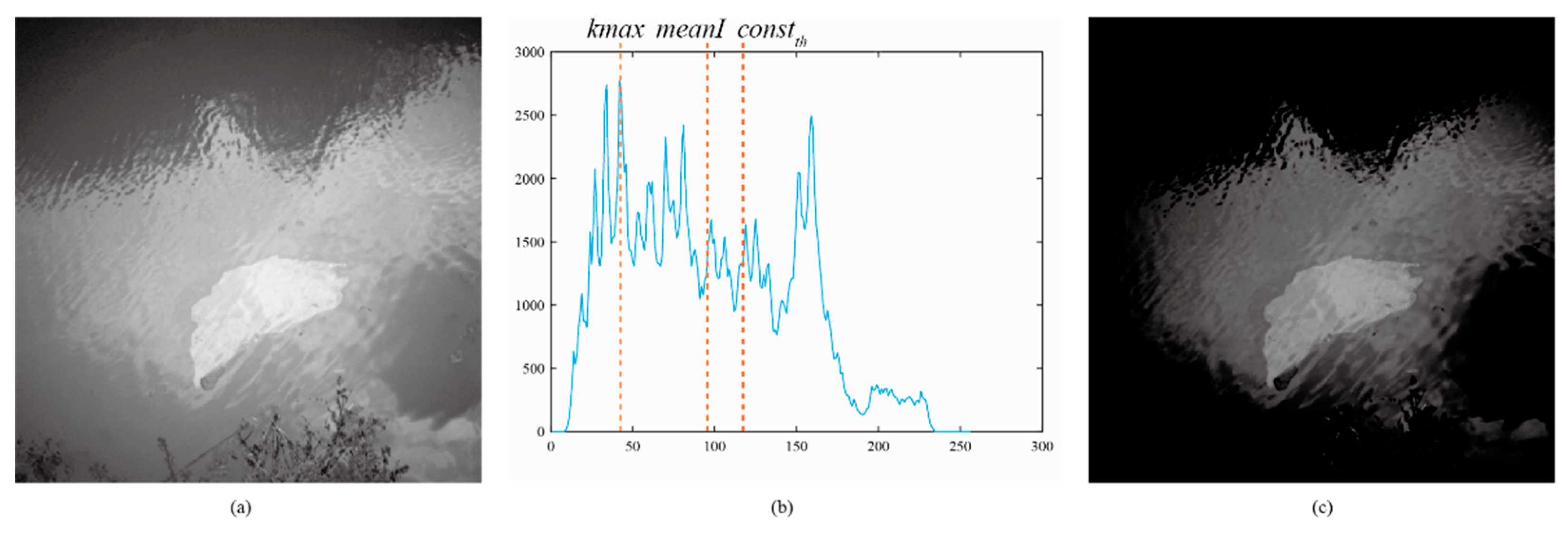
(1) Calculate the average intensity values meanI of image I and the corresponding intensity value kmax of the peak of the histogram. kmax is determined using the following equation:
where hist(k) is the histogram and k is the intensity value ranging from 0 to 255.
(2) In the extreme illumination situation, such as when the image is overexposed, the above two values cannot acceptably suppress the background, and so we added a constant thresholding constth for all images. In this work, constth =120 is a reasonable selection. As the size of the dataset increases, this value can be optimized.
(3) Sort meanI, kmax, and constth, and choose the median number as the background threshold bth, as in the following:
(4) Subtract bth from the image and set it to zero. If the pixel intensity value is less than or equals to bth, it remains 0. Otherwise, set the value as I(i,j) − bth, which is expressed as follows:
where I(i,j) is the pixel intensity of the ith row and jth column of the original image I, and Igbs(i,j) is the processed pixel intensity value.
Due to different imaging conditions, the area occupied by the target and the imaging light in each image are different, which will affect the meanI and kmax of the whole image. When considering the values of the above three numbers, it is reasonable to choose the median. Figure 5 demonstrates an example using GBS.
2.2.2. Adaptive Target Enhancement
To compensate for the intensity decay caused by the above intensity subtraction, an algorithm for enhancing the saliency of the target, which is called adaptive target enhancement (ATE), is proposed. ATE allocates an individual weight for each pixel, as shown in Equation (4):
where Ri is the variant in the ith row of the image, mRi is the mean value of R, H is the height of the image, λi is the intensity enhancement coefficient vector of the ith row, and Iate is the result of the ATE.
From Equation (4), the key point of ATE is that the weight value should be small when the pixel belongs to the target area, while the weight value should be large when the pixel belongs to the nontarget area. In our preprocessed image dataset, the target is brighter than its surrounding background, and it has a sharp edge that outlines its shape. Meanwhile, the background is without these distinct features. According to these characteristics, we combine the intensity value, the local information entropy, and the gradient information to estimate the weight for each pixel of the image. The adaptive weight calculation procedure can be briefly summarized into the following steps.
(1) The mean intensity value and standard deviation of the ith row, i.e., mRi and stdRi, respectively, are calculated.
(2) According to stdRi, we assign a coefficient η to mRi, where η is determined by the following equation:
In a row with a high intensity value and standard deviation, there is low confidence in the target as well, and here we assign a large η. Otherwise, we assign a small η. th1 = 15, η1 = 1, and η2 = 0.8 in this work.
(3) The Sobel operator is used to generate the gradient image G, and scale the gradient value of the data to [0,1].
(4) The local entropy value of the 8 neighbors around the corresponding pixel in the input image is calculated to get the local entropy image E. A threshold th2 is set, which equals 0.65 × max(E). If E(i,j) < th2 is satisfied, this entropy value is set to zero; otherwise, the present value is retained. Then, the entropy value of data is scaled to [0,1].
(5) The weight λ(i,j) for each pixel in the ith row and jth column is calculated as follows:
Here, sgn is the sign function, which is defined as follows:
I(i,j), E(i,j), and G(i,j) represent the intensity value, local entropy value, and gradient value at position (i,j), respectively. Figure 6 presents the result of the ATE algorithm. After this step, the target area and the background area have a clear distinction. To extract the target area from the processed image, clustering segmentation is an effective method that can be applied.
2.2.3. Histogram-Based Determination of the Optimal Number of Clusters
The performance of the next segmentation algorithm highly depends on the initial number of clusters. The automatic determination of the number of clusters is of great significance in cluster analysis. To solve this problem, we analyze the histogram distribution features in order to evaluate the different areas in the image, which will provide an approach to generate the optimal number of clusters.
The automatic number selection procedure has five steps.
(1) Detect all local maxima, which means to find the peak heights Hk in the histogram.
(2) Find the global maximum counts and set the height threshold th3 as follows:
(3) Calculate the prominence values Pk from the candidate maxima. The prominence value is the minimum vertical distance that the signal must descend on either side of the peak before either climbing back to a level higher than the peak or reaching an endpoint. Set the prominence threshold th4 = 75.
(4) Calculate the distances Wk between the peaks. Set a distance threshold th5 = 8, choose the tallest peak in the histogram, and ignore all peaks within the distance.
(5) The peaks that are more than or equal to th3, th4, and th5 are kept. Then, map the number of these peaks Npk into the set {n, n+1} according to the following conditions:
where N is the result of the optimal number of clusters for this image, and n = 3 in our work.
Figure 7 further explains the above steps. The blue triangles indicate the location of each peak. The orange lines that are vertical to the horizontal axis represent the height of each peak, and the green line that is vertical to the magenta horizontal line is the prominence value of each peak. If Hk > th3, Wk > th4, and Pk > th5, this peak will remain (the red triangles in Figure 7), and otherwise it will be discarded (the blue triangles in Figure 7). From the observation of the processed images, we can see that the images always contain water regions, chemical spill regions, and other regions. Sometimes, the difference between water background and target areas is so subtle that we need a more detailed division. Based on that, the suitable number of clusters is determined to be between 3 and 4. This step helps to improve the automation of our algorithm.
2.2.4. Local Fuzzy Thresholding Segmentation
After the number of clusters is determined, a multiregion image segmentation algorithm, which is called the local fuzzy thresholding methodology (LFTM) and was proposed in [33], is applied to precisely segment a region of interest (ROI). Compared to common fuzzy-based approaches, this method will take advantage of the use of fuzzy membership degrees and the spatial relations, which helps to overcome noise-related problems, uneven illumination, and soft transitions between gray levels. In our work, the number of centroids refers to the number of clusters, which is determined in Section 2.2.3; the type of local information aggregation is the Median Max aggregation; and the local window size is 3 × 3. More details about this algorithm can be found in [33]. The LFTM processed result is an image with L values, where L is the number of regions. We then convert it to a binary result, and based on the threshold, it equals L_1.
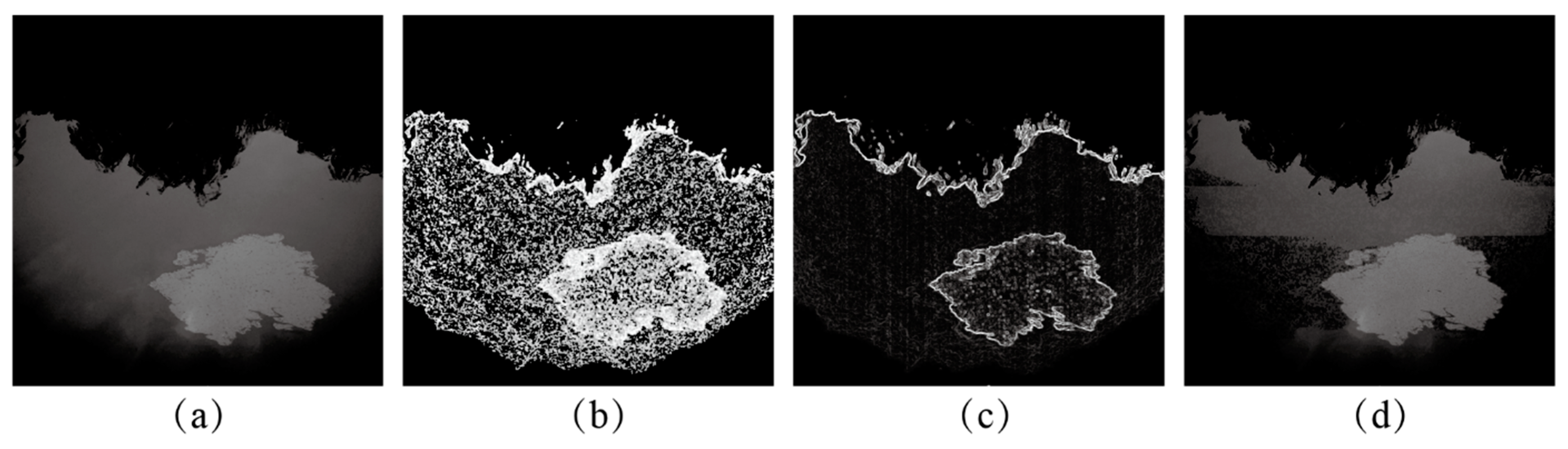
Several segmentation examples before and after target enhancement are shown in Figure 8. It is obvious that the LFTM generally extracts the target from the background with frequent commissions. The GBS and ATE processed images can be correctly segmented by the LFTM, except for some omissions of the boundary parts and the inclusion of the highlighted parts.
2.3. Post-Segmentation Processing
The regions that are segmented by the above steps may contain small undetected holes and misclassified objects (Figure 8b). To remove these nontarget objects from the candidates, we conducted a post-segmentation process. First, we filled the holes within the connected components and calculated the area of each component. Areas that were smaller than 400 pixels were removed in order to reduce the small misclassified objects and noises. Second, we calculated the ratio of the width to the length (w/l) of the candidates. For a spill target, the bounding box with the minimum area usually has a large w/l. Considering special situations, such as the small w/l of a small spill caused by windy weather, we removed the candidates with w/ls less than 0.3 and areas below 800 pixels. Finally, if there was only one candidate left, we ended the process; otherwise, we calculated the textural feature of the candidates. The textural feature is the standard deviation of the gradient of the connected area boundary in the original image. Standard deviations above 55 were removed accordingly. This step further improved the segmentation accuracy.
3. Experimental Results and Discussion
3.1. Colorless Xylene Spill Image Acquisition
We acquired xylene spill images by performing an outdoor experiment to investigate xylene spills under clear sky conditions. The experiment was carried out at an artificial channel on the campus of Ocean College at Zhejiang University in Zhoushan, Zhejiang, China. The wind speed was 2–3 m/s. Xylene is one of the top 10 chemicals that is likely to pose the highest risk of being involved in an HNS incident, and it is a typical benzene series. The xylene that was used in our experiment was produced by Aladdin, Shanghai. Approximately 30 mL of xylene was released into the channel each time. A hand-held digital camera (a6000, Sony, Japan) equipped with an ultraviolet narrow bandpass filter (365 nm) with an observation angle ~30 from the zenith and ~5 m away from the xylene spill targets was used to capture the UV images under different scenarios, including shadows, waves, and sun reflections. The camera has a 16–50 mm Sony lens, generates an 8-bit gray level image with a resolution of 4000 × 4000, and covers a scope of approximately 6 × 6 m2 in one shoot. The exposure time is 1/50 s. The UV images were taken 30 s after all the xylene was dispensed, thus allowing enough time for the liquid spills to stabilize. We conducted this experiment with full protection and cleaned up all chemicals following Regulation on the Safety Management of Hazardous Chemicals [38].
The dataset (53 images) consists of a series of images containing chemical spill targets in different background conditions. The proposed algorithm is implemented by MATLAB code, runs on the Ubuntu 18.04 operating system with an Intel Core i5-4750 processor, 3.2GHZ, and 16.00GB RAM.
3.2. UV Image Processing Results
We applied the proposed approach to several UV images using the configuration of parameters that was given in the above section. These values that were in Section 2 were optimized and tuned according to the tested UV images with the goal of achieving satisfactory detection results. Figure 9, Figure 10 and Figure 11 show several segmentation examples of the chemical spill.
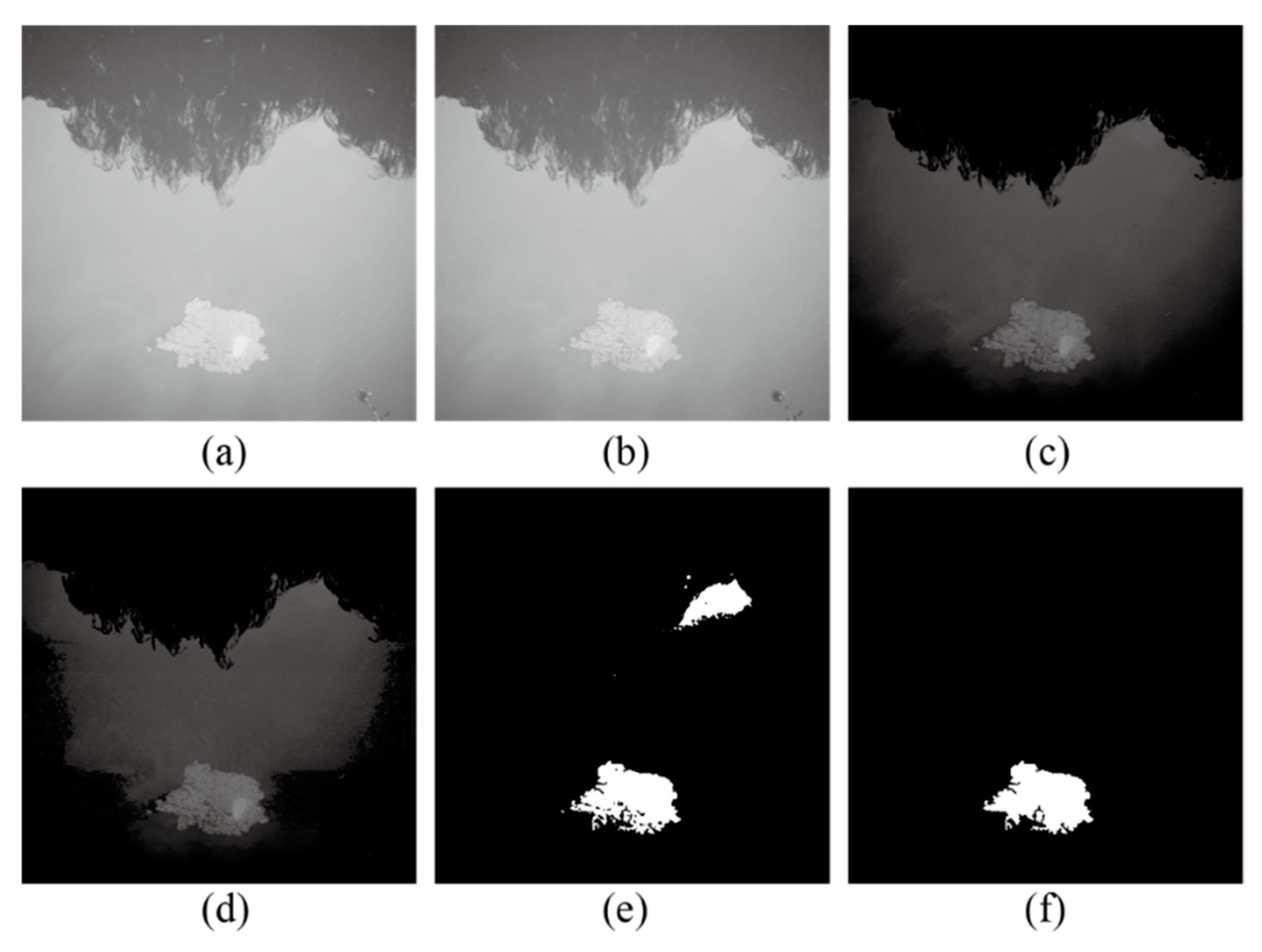
In Figure 9, the spill target in the original UV image looks like a small bright spot with a vaguely visible outline while the top of the water background is covered by shadows, and the low part has a similar gray value to the target area. Figure 9b shows the result after the preprocessing with the decreased resolution. Figure 9c,d are the results of the GBS and ATE, respectively. The optimal number of clusters was automatically set to 4 by analyzing the histogram information of Figure 9d. Figure 9e shows the segmentation results after the LFTM (cluster number = 4). Figure 9f shows the final segmented spill target after postprocessing. It is obvious that GBS and ATE do suppress the background interference and enhance the target area. The LFTM helps us to segment candidate target regions from the processed images. Then, with the evaluation of the LFTM-proposed candidates, we finally distinguished the correct spill target from the background.
Figure 10 illustrates the full segmentation process of a UV image with strong waves where the spill target is surrounded by a rough water surface. The waves critically interfere with the segmentation of the spill targets. An original image is presented in Figure 10a. The reflections formed by the waves are randomly scattered in the image. Figure 10b is the result after preprocessing. The background suppression and target enhancement processing results are shown in Figure 10c,d. The optimal number of clusters is set using the proposed method. The segmentation results after the LFTM are presented in Figure 10e. The result of the target classification without the other interference, such as sun reflections, is shown in Figure 10f. It is shown that the main target has been accurately identified, but the details of the boundary cannot be successfully segmented because of their weak feature. Chemical on water surface has a thin and heterogeneous liquid film, which when interacting with the wave, breaks the edge of spill to many fractal edge structures, as emphasized in left-down part of Figure 10d. Along with uneven illumination, the edge and spill area shows heterogeneous contrast to water, which caused pixel misclassification, as shown in Figure 10e. Small areas were abandoned by postprocessing to remain the integrity of segmented area. This would be the reason that the area in Figure 10f is smaller than the true spill area.
Figure 11 shows the processing sequence that was applied to a UV image under uneven illumination with water ripples and shrub branches. In Figure 11a, we can see that the spill target is in the right middle of the image and is surrounded by a bright background. Figure 11b is the result after preprocessing. After GBS and ATE are applied, the difference between the target region and the surrounding environment becomes detectable, as shown in Figure 11c,d. After cluster number analysis, it is reasonable to divide the picture into four clusters, i.e., cluster number is set to 4. The LFTM segmentation result is shown in Figure 11e. The post-segmentation processing discards the background noise and selects the right target. The final segmentation result is demonstrated in Figure 11f. The shape of the right edge corresponds with the edge of the shadow at the right side of the spill. This may be the reason that these pixels were misclassified.
Our aim is to segment the spill target from the UV image. The above three examples verify that our proposed algorithm is effective and robust under different scenarios, such as low contrast, wave reflections, and uneven illumination. According to the gray intensity feature, the edge gradient information feature, the local information entropy feature, and the spatial distribution feature of the chemical spill area, this method helps us to deal with the segmentation tasks in different backgrounds and to achieve promising results.
3.3. Comparison with Other Methods
To verify the performance of our method, we compare it with other five segmentation approaches: Otsu (Otsu) [27], maximum entropy (Max entropy) [28], the Chan–Vese active contour model (CV model) [39], and two LFTMs [33]. The parameters of each method are tuned through multiple experiments in order to get reasonable results. To better objectively evaluate all these methods, quantitative evaluations are performed using four measurements: the Accuracy (AC), Precision (PR), Recall (RE), and F1 score (F1). The metrics are defined as follows:
where True Positives (TP) are the number of pixels that are correctly detected as target pixels, False Negatives (FN) are the number of pixels that are incorrectly classified as background pixels, True Negatives (TN) are the number of pixels that are correctly recognized as background pixels, and False Positives (FP) are the number of pixels that are incorrectly classified as target pixels. AC is the ratio of misclassified pixels to all pixels. PR is the ratio of the correctly detected target pixels to the total number of target pixels in the image. RE measures the ratio of the correctly detected target pixels to the total pixels of target region in the image. F1 is the harmonic average of the PR and RE.
The segmentation results of different methods are presented in Figure 12. Otsu and Max entropies are fully automatic methods without parameter setting. Original LFTM needs to be set with the initial number of clusters, which are set to 3 and 4 here, respectively. CV model needs to set the iteration times and initial state of the active contour, which set to 500 and a bounding box with (xmin: 100, ymin: 100, xmax: 300, ymax: 300), respectively. Our proposed method yields more satisfactory results than the other methods. Since there is no standard reference for our own dataset, we have to manually label the target from the test image. The ground-truth (Figure 12h) is segmented manually including all the pixels belonging to the region that is considered as a true xylene spill.
As shown in Figure 12, a large number of background pixels are classified as targets by the Otsu, Max entropy, and CV models, thereby resulting in high FPs. The LFTM avoids part of the misclassification and acquires a moderate FP. The above methods sacrifice accuracy in order to achieve a high recall. Our method correctly finds the majority of the targets with an extremely low FP, which indicates that our algorithm balances the accuracy and recall.
The average quantitative evaluation measures (AC, PR, RE, and F1) of all the segmented images by each method are obtained by comparing the automatic segmentation results (Figure 12b–g) with the ground-truth. The results along with average time are listed in Table 1 to evaluate the performance of each method. In Table 1, it is obvious that our algorithm achieves the highest accuracy (AC), precision (PR), and F1 score, and a relatively high recall (RE). The comparison results show that our method has its strengths in finding “real” targets (higher accuracy and precision values) and limitations in its detection sensitivity (relatively lower recall values). With respect to the on-site detection of floating HNS spills, a large number of false positives will waste emergency rescue resources. Both the qualitative (Figure 12) and quantitative (Table 1) analyses indicate that our method achieves superior performance to other methods. Especially by comparing the result between our method and the LFTM, the GBS and ATE that are proposed in this paper make great contributions in discriminating spill targets from background through image features including the intensity, entropy, and gradient features. In addition, the post-segmentation process also helps to remove nontarget pixels.
The computational time of our method for one image is 1.6609 s, a little longer than 0.9381 s using LFTM with Ncluster = 3, while less than 1.8395 s using LFTM with Ncluster = 4. It is indicated that computational time increases with the increase of the number of clusters of LFTM. The overall precision of our method is better than other methods and original LFTM. Although our method is slower than the Otsu and max entropy, the computational time is still about 1.5 s on average, and the precision is much better. Hence, our method is suitable for the chemical spill area detection.
After segmentation by the above method, each pixel can be classified. These classified pixels can be used for target information statistics. Applying this method to high-precision remote sensing images acquired by UAV, combined with the flight data, we can calculate the spill area and support emergency strategy for spill incident.
3.4. The Effect of Parameter Setting
We also tested various parameter settings to assess the segmentation stability of the proposed method. As mentioned above, there are 7 parameters (constth, th1, η2, th3, th4, th5, texture_std) in our method, while area and w/l are geometric features of candidate images. We adjusted each parameter and compared the results with ground truth to calculate the F1 scores. The average results are shown in Table 2, where the proposed method obtains a minimum F1 score of 0.8394, which implies that the workflow performs consistently well for a variety of parameters setting.
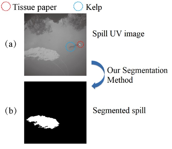
3.5. Performance on UV Images Containing Interferents
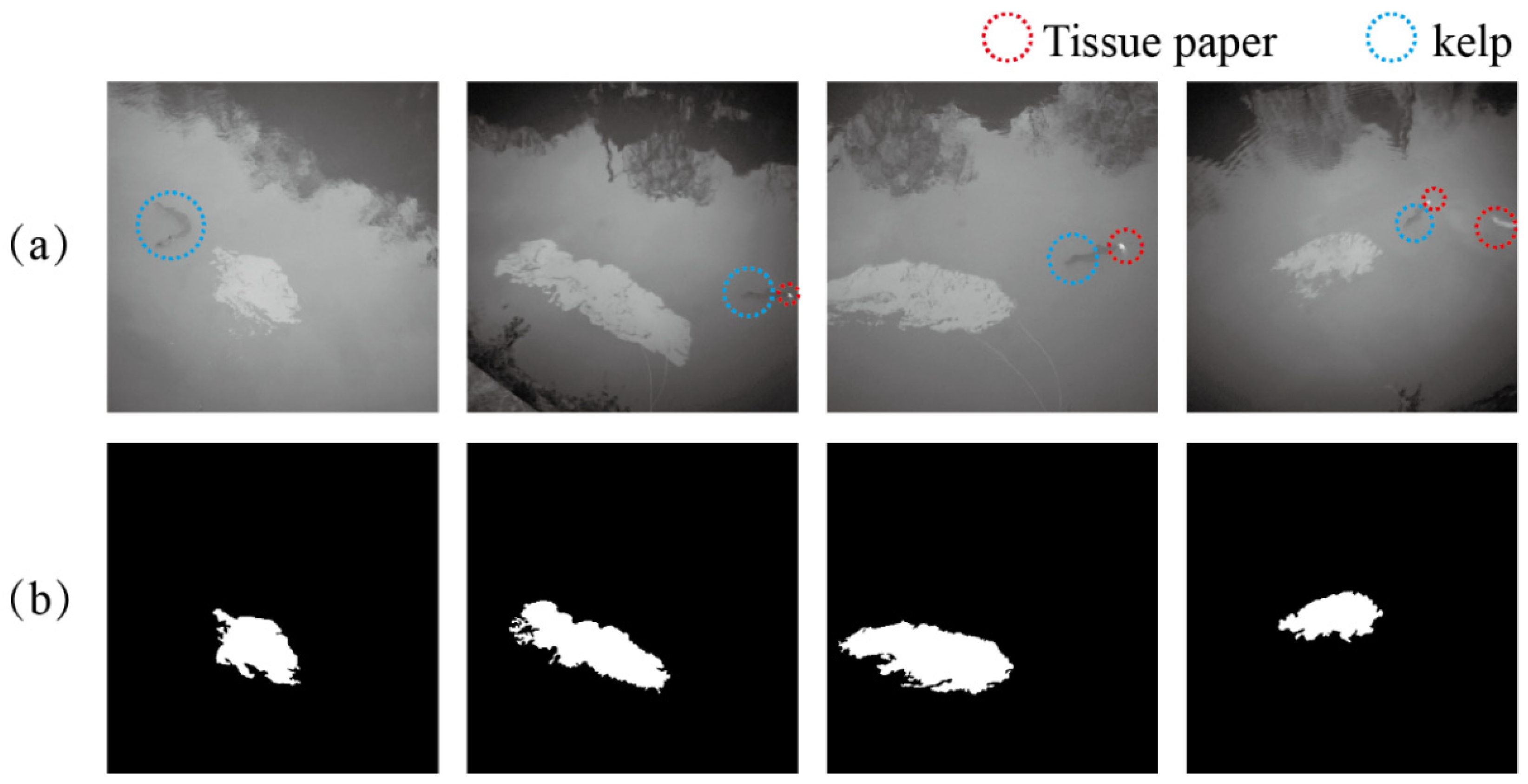
It is necessary to study the influence of interferents on the approach. We captured 20 UV images with tissue paper and kelp by the camera described in Section 3.1 and applied our method on these images. AC, PR, RE, and F1 of 0.9686, 0.8891, 0.6812, and 0.7578, respectively, were obtained for our method. Examples of segmentation results are shown in Figure 13. When the interferent is small, e.g., the tissue paper or its gray value is low in the UV band, the proposed method can recognize the true target. Our method gets F1 score of 0.7575, which is better than 0.2917 when using original LFTM with Ncluster = 3, and 0.3704 when using original LFTM with Ncluster = 4, while indicator of RE is slightly lower than the other two methods. The edge of some targets is blurred due to the fast movement of chemical spill. This could cause error in the step of ATE resulting in relatively lower RE and F1 scores.
As discussed above, our method is suitable for the spill segmentation in UV images with interferent. We believe that with improvement based on a large and elaborated dataset, our method will be more applicable for the segmentation in remote sensing detection of chemical spill.
4. Conclusions
In this paper, we present an effective and robust method for automatically extracting xylene spill target from UV images. We proposed an advanced LFTM, which determines cluster numbers automatically and adaptively based on histogram analysis, as the performance of clustering-based segmentation methods highly relies on the selection of the number of clusters. Combining gray value, gradient value, and entropy value, we designed an ATE incorporated by GBS, by which unapparent spill target regions become detectable in UV images with waves, sun reflections, low contrast, and uneven illumination, and hence improve the segmentation precision using LFTM. The whole workflow in this paper should be seen as a basic frame rather than a closed algorithm, and each step can be displaced or replaced by equivalent operations. Due to the use of GBS and ATE, our method loses some local image details which leads to room for improvement in the recall of our method. This is one of our next research focuses.
Parameters (constth, th1, η2, th3, th4, th5, texture_std) and target selection thresholds are experimentally determined and optimized. The proposed method demonstrated its promising detecting capability on UV images with waves, sun reflections, low contrast, and uneven illumination. The overall detecting precision (indicator of F1) of the proposed algorithm is better than the method using original LFTM and other thresholding methods such as Ostu, max entropy, and CV model. Results on current database show a trend of mild increase in computational complexity, along with the increase of accuracy. We also applied our method on UV images with inteferents, e.g., tissue paper and kelp. The result demonstrates that our method is suitable for the segmentation of images with look-alike objects.
To develop the method, increase in the size of the dataset may be helpful on robustness, parameter optimization, and reduction of computational complexity. In the future, more images of large-scale chemical spills captured by moving platforms, e.g., UAVs will be collected to improve our algorithms for in situ remote sensing detection.
Author Contributions
For research articles with several authors, a short paragraph specifying their individual contributions must be provided. The following statements should be used “Conceptualization, S.Z. and C.W.; Methodology, C.W.; Software, S.L.; Validation, S.L., K.X. and C.W.; Formal Analysis, S.Z.; Investigation, C.W.; Resources, C.L.; Data Curation, S.Z.; Writing-Original Draft Preparation, S.Z.; Writing-Review & Editing, H.H.; Visualization, S.L.; Supervision, R.X.; Project Administration, C.L.; Funding Acquisition, R.X.
Funding
This work was financially supported by the National Natural Science Foundation of China (grant number: 31801619, 61605169), National Key R&D Program of China (grant number: 2016YFC1402403), and Natural Science Foundation of Zhejiang Province (grant number: Y18F050010).
Acknowledgments
In this section you can acknowledge any support given which is not covered by the author contribution or funding sections. This may include administrative and technical support, or donations in kind (e.g. materials used for experiments).
Conflicts of Interest
The authors declare no conflict of interest.
References
- Purnell, K. Are HNS spills more dangerous than oil spills. In Proceedings of the A white paper for the interspill conference & the 4th IMO R&D Forum, Marseille, France, May 2009; pp. 12–14. [Google Scholar]
- International Maritime Organization (IMO). Protocol on Preparedness, Response and Co-Operation to Pollution Incidents by Hazardous and Noxious Substances (OPRC-HNS Protocol); IMO: London, UK, 2000. [Google Scholar]
- Cunha, I.; Moreira, S.; Santos, M.M. Review on hazardous and noxious substances (HNS) involved in marine spill incidents-An online database. J. Hazard. Mater. 2015, 285, 509–516. [Google Scholar] [CrossRef] [PubMed]
- Cunha, I.; Oliveira, H.; Neuparth, T.; Torres, T.; Santos, M.M. Fate, behaviour and weathering of priority HNS in the marine environment: An online tool. Mar. Pollut. Bull. 2016, 111, 330–338. [Google Scholar] [CrossRef] [PubMed]
- Yim, U.H.; Kim, M.; Ha, S.Y.; Kim, S.; Shim, W.J. Oil Spill Environmental Forensics: The Hebei Spirit Oil Spill Case. Environ. Sci. Technol. 2012, 46, 6431–6437. [Google Scholar] [CrossRef] [PubMed]
- International Tanker Owners Pollution Federation Limited (ITOPF). TIP 17: Response to Marine Chemical Incidents, Technical Information Papers; ITOPF: Copenhagen, Denmark, 2014; pp. 3–4. [Google Scholar]
- Moriarty, J.; Schwartz, L.; Tuck, E. Unsteady spreading of thin liquid films with small surface tension. Phys. Fluids A Fluid Dyn. 1991, 3, 733–742. [Google Scholar] [CrossRef]
- Angelliaume, S.; Minchew, B.; Chataing, S.; Martineau, P.; Miegebielle, V. Multifrequency radar imagery and characterization of hazardous and noxious substances at sea. IEEE Trans. Geosci. Remote 2017, 55, 3051–3066. [Google Scholar] [CrossRef]
- Zhao, J.; Temimi, M.; Ghedira, H.; Hu, C. Exploring the potential of optical remote sensing for oil spill detection in shallow coastal waters-a case study in the Arabian Gulf. Opt. Express 2014, 22, 13755–13772. [Google Scholar] [CrossRef]
- Taravat, A.; Del Frate, F. Development of band ratioing algorithms and neural networks to detection of oil spills using Landsat ETM+ data. EURASIP J. Adv. Signal Process. 2012, 2012, 1687–6180. [Google Scholar] [CrossRef]
- Conmy, R.N.; Coble, P.G.; Farr, J.; Wood, A.M.; Lee, K.; Pegau, W.S.; Walsh, I.D.; Koch, C.R.; Abercrombie, M.I.; Miles, M.S. Submersible optical sensors exposed to chemically dispersed crude oil: Wave tank simulations for improved oil spill monitoring. Environ. Sci. Technol. 2014, 48, 1803–1810. [Google Scholar] [CrossRef] [PubMed]
- Fingas, M.; Brown, C.E. Oil spill remote sensing: A review. In Oil Spill Science and Technology; Elsevier: Amsterdam, The Netherlands, 2011; pp. 111–169. [Google Scholar]
- Martin, C.; Parkes, S.; Zhang, Q.; Zhang, X.; McCabe, M.F.; Duarte, C.M. Use of unmanned aerial vehicles for efficient beach litter monitoring. Mar. Pollut. Bull. 2018, 131, 662–673. [Google Scholar] [CrossRef] [PubMed]
- Turner, I.L.; Harley, M.D.; Drummond, C.D. UAVs for coastal surveying. Coast. Eng. 2016, 114, 19–24. [Google Scholar] [CrossRef]
- Papakonstantinou, A.; Topouzelis, K.; Pavlogeorgatos, G. Coastline zones identification and 3D coastal mapping using UAV spatial data. ISPRS Int. J. Geo-Inf. 2016, 5, 75. [Google Scholar] [CrossRef]
- Ma, X.; Cheng, Y.; Hao, S. Multi-stage classification method oriented to aerial image based on low-rank recovery and multi-feature fusion sparse representation. Appl. Opt. 2016, 55, 10038–10044. [Google Scholar] [CrossRef]
- Solberg, A.H.S.; Storvik, G.; Solberg, R.; Volden, E. Automatic detection of oil spills in ERS SAR images. IEEE Trans. Geosci. Remote 1999, 37, 1916–1924. [Google Scholar] [CrossRef]
- Karantzalos, K.; Argialas, D. Automatic detection and tracking of oil spills in SAR imagery with level set segmentation. Int. J. Remote Sens. 2008, 29, 6281–6296. [Google Scholar] [CrossRef]
- Jing, Y.; An, J.; Liu, Z. A novel edge detection algorithm based on global minimization active contour model for oil slick infrared aerial image. IEEE Trans. Geosci. Remote 2011, 49, 2005–2013. [Google Scholar] [CrossRef]
- Yang, M.; Song, W.; Mei, H. Efficient Retrieval of Massive Ocean Remote Sensing Images via a Cloud-Based Mean-Shift Algorithm. Sensors 2017, 17, 1693. [Google Scholar] [CrossRef]
- Dolenko, T.A.; Fadeev, V.V.; Gerdova, I.V.; Dolenko, S.A.; Reuter, R. Fluorescence diagnostics of oil pollution in coastal marine waters by use of artificial neural networks. Appl. Opt. 2002, 41, 5155–5166. [Google Scholar] [CrossRef]
- Wang, X.-F.; Min, H.; Zou, L.; Zhang, Y.-G. A novel level set method for image segmentation by incorporating local statistical analysis and global similarity measurement. Pattern Recogn. 2015, 48, 189–204. [Google Scholar] [CrossRef]
- Zhang, K.; Song, H.; Zhang, L. Active contours driven by local image fitting energy. Pattern Recogn. 2010, 43, 1199–1206. [Google Scholar] [CrossRef]
- Wang, P.; Lee, D.; Gray, A.; Rehg, J.M. Fast mean shift with accurate and stable convergence. In Proceedings of the Eleventh International Conference on Artificial Intelligence and Statistics, Palo Alto, CA, USA, 4–8 June 2007; pp. 604–611. [Google Scholar]
- Nieto-Hidalgo, M.; Gallego, A.-J.; Gil, P.; Pertusa, A. Two-stage convolutional neural network for ship and spill detection using SLAR images. IEEE Trans. Geosci. Remote 2018, 56, 5217–5230. [Google Scholar] [CrossRef]
- Xu, L.; Javad Shafiee, M.; Wong, A.; Li, F.; Wang, L.; Clausi, D. Oil spill candidate detection from SAR imagery using a thresholding-guided stochastic fully-connected conditional random field model. In Proceedings of the IEEE Conference on Computer Vision and Pattern Recognition Workshops, Boston, MA, USA, 7–12 June 2015; pp. 79–86. [Google Scholar]
- Otsu, N. A threshold selection method from gray-level histograms. IEEE Trans. Syst. Man Cybern. 1979, 9, 62–66. [Google Scholar] [CrossRef]
- Wong, A.K.; Sahoo, P.K. A gray-level threshold selection method based on maximum entropy principle. IEEE Trans. Syst. Man Cybern. 1989, 19, 866–871. [Google Scholar] [CrossRef]
- Pham, D.L.; Prince, J.L. An adaptive fuzzy C-means algorithm for image segmentation in the presence of intensity inhomogeneities. Pattern Recognit. Lett. 1999, 20, 57–68. [Google Scholar] [CrossRef]
- Bradley, D.; Roth, G. Adaptive thresholding using the integral image. J. Graph. Tools 2007, 12, 13–21. [Google Scholar] [CrossRef]
- Du, F.; Shi, W.; Chen, L.; Deng, Y.; Zhu, Z. Infrared image segmentation with 2-D maximum entropy method based on particle swarm optimization (PSO). Pattern Recognit. Lett. 2005, 26, 597–603. [Google Scholar]
- Chuang, K.-S.; Tzeng, H.-L.; Chen, S.; Wu, J.; Chen, T.-J. Fuzzy c-means clustering with spatial information for image segmentation. Comput. Med. Imaging Graph. 2006, 30, 9–15. [Google Scholar] [CrossRef]
- Aja-Fernández, S.; Curiale, A.H.; Vegas-Sánchez-Ferrero, G. A local fuzzy thresholding methodology for multiregion image segmentation. Knowl. Based Syst. 2015, 83, 1–12. [Google Scholar] [CrossRef]
- Huang, Y.; Xu, B. Automatic inspection of pavement cracking distress. J. Electron. Imaging 2006, 15, 13–17. [Google Scholar] [CrossRef]
- Tomasi, C.; Manduchi, R. Bilateral filtering for gray and color images. In Proceedings of the Sixth International Conference on Computer Vision, Bombay, India, 7 January 1998; pp. 839–846. [Google Scholar]
- Liu, C.; Freeman, W.T.; Szeliski, R.; Kang, S.B. Noise estimation from a single image. In Proceedings of the 2006 IEEE Computer Society Conference on Computer Vision and Pattern Recognition, New York, NY, USA, 17–22 June 2016; pp. 901–908. [Google Scholar]
- Perona, P.; Malik, J. Scale-space and edge detection using anisotropic diffusion. IEEE Trans. Pattern Anal. Mach. Intell. 1990, 12, 629–639. [Google Scholar] [CrossRef]
- General Office of the State Council. Regulation on the Safety Management of Hazardous Chemicals (2011 version); Order No.591 of the State Council; General Office of the State Council: Beijing, China, 2011.
- Chan, T.; Vese, L. An active contour model without edges. In Proceedings of the International Conference on Scale-Space Theories in Computer Vision, Corfu, Greece, 26–27 September 1999; pp. 141–151. [Google Scholar]
Figure 1.
Workflow of the proposed method.

Figure 2.
An example of the grid cell analysis (GCA) process.

Figure 3.
An example of the pre-segmentation processing—(a) original image (4000 × 4000) and (b) processed image (500 × 500).
Figure 3.
An example of the pre-segmentation processing—(a) original image (4000 × 4000) and (b) processed image (500 × 500).

Figure 4.
Examples of chemical spill targets in UV images. (a) Image with shadow; (b) image with shadow, wave, and sun reflection; (c) image with shadow, wave, and sun reflection;Since a complex background is not conducive to the precise segmentation of the target, we propose a global background suppression (GBS) algorithm to subtract the redundant information from the background. The main idea of the algorithm is to estimate an adjustable threshold based on the intensity distribution, and then to filter the pixels that are less than the threshold in the images. The details are described as follows.

Figure 5.
An example of the result of global background suppression (GBS). (a) The original image; (b) the three candidate threshold values; and (c) the global background suppression result.
Figure 5.
An example of the result of global background suppression (GBS). (a) The original image; (b) the three candidate threshold values; and (c) the global background suppression result.

Figure 6.
An example of the result of adaptive target enhancement (ATE). (a) The original image; (b) the local entropy image; (c) the gradient image; and (d) the ATE result.
Figure 6.
An example of the result of adaptive target enhancement (ATE). (a) The original image; (b) the local entropy image; (c) the gradient image; and (d) the ATE result.

Figure 7.
A diagram of the peak heights, prominence value, and distance value within the histogram.

Figure 8.
Examples of segmentation results. (a) The original images; (b) the results after GBS, ATE, and LFTM; (c) the results using only local fuzzy thresholding methodology (LFTM) with 3 centroids; and (d) the results using only LFTM with 4 centroids.
Figure 8.
Examples of segmentation results. (a) The original images; (b) the results after GBS, ATE, and LFTM; (c) the results using only local fuzzy thresholding methodology (LFTM) with 3 centroids; and (d) the results using only LFTM with 4 centroids.

Figure 9.
Segmentation result of a small target with shadows. (a) The original image (4000 × 4000); (b) the preprocessed image (500 × 500); (c) the result using GBS; (d) the result using ATE; (e) the segmentation result with LFTM; and (f) the final segmentation result.
Figure 9.
Segmentation result of a small target with shadows. (a) The original image (4000 × 4000); (b) the preprocessed image (500 × 500); (c) the result using GBS; (d) the result using ATE; (e) the segmentation result with LFTM; and (f) the final segmentation result.

Figure 10.
Segmentation result of a target with low contrast and waves. (a) The original image; (b) the preprocessed image; (c) the result using GBS; (d) the result using ATE; (e) the segmentation result with LFTM; and (f) the final segmentation result.
Figure 10.
Segmentation result of a target with low contrast and waves. (a) The original image; (b) the preprocessed image; (c) the result using GBS; (d) the result using ATE; (e) the segmentation result with LFTM; and (f) the final segmentation result.

Figure 11.
Segmentation result of a target uneven illumination. (a) The original image; (b) the preprocessed image; (c) the result using GBS; (d) the result using ATE; (e) the segmentation result with LFTM; and (f) the final segmentation result.
Figure 11.
Segmentation result of a target uneven illumination. (a) The original image; (b) the preprocessed image; (c) the result using GBS; (d) the result using ATE; (e) the segmentation result with LFTM; and (f) the final segmentation result.

Figure 12.
Comparison results. (a) Original image; (b) Otsu; (c) Max entropy; (d) LFTM with Ncluster = 3; (e) LFTM with Ncluster = 3; (f) Chan–Vese active contour model (CV model); (g) our method; and (h) ground-truth.
Figure 12.
Comparison results. (a) Original image; (b) Otsu; (c) Max entropy; (d) LFTM with Ncluster = 3; (e) LFTM with Ncluster = 3; (f) Chan–Vese active contour model (CV model); (g) our method; and (h) ground-truth.

Figure 13.
Segmentation result of UV images containing interferents. (a) Original UV images and (b) results using our method.
Figure 13.
Segmentation result of UV images containing interferents. (a) Original UV images and (b) results using our method.


Table 1.
Quantitative comparison results of the different segmentation methods.
| Method | AC | PR | RE | F1 | Average Time(s) |
|---|---|---|---|---|---|
| Otsu | 0.5493 | 0.2214 | 0.9957 | 0.3401 | 0.0044 |
| Max entropy | 0.5879 | 0.2546 | 0.9736 | 0.3713 | 0.0073 |
| LFTM with Ncluster = 3 | 0.8240 | 0.4624 | 0.9681 | 0.5700 | 0.9381 |
| LFTM with Ncluster = 4 | 0.9203 | 0.6700 | 0.9098 | 0.7226 | 1.8395 |
| CV model | 0.5826 | 0.2408 | 0.9952 | 0.3585 | 7.5594 |
| Our method | 0.9679 | 0.9497 | 0.8112 | 0.8614 | 1.6609 |
The bold text shows the best result for each column.
Table 2.
The result of different parameters setting.
| Process | Parameter | Variation Settings a | F1 Score Result (Mean/SD) |
|---|---|---|---|
| GBS | constth | 90, 100, 110, 120, 130, 140, 150 | 0.8478/0.0172 |
| ATE | th1 | 5, 10, 15, 20, 25, 30, 35 | 0.8601/0.0051 |
| th2 | (0.45, 0.55, 0.65, 0.75, 0.85) × max(E) | 0.8481/0.00841 | |
| η2 | 0.4, 0.6, 0.8, 0.9 | 0.8523/0.0079 | |
| Automatic select clusters | th4 | 55, 65, 75, 85, 95 | 0.8613/0.0025 |
| th5 | 4, 8, 16, 32 | 0.8394/0.0214 | |
| Post-segmentation processing | area | – | – |
| w/l | – | – | |
| texture_std | 45, 55, 65, 75, 85 | 0.8404/0.0390 |
a the bold font in variation settings column are the selected parameters in manuscript.
© 2019 by the authors. Licensee MDPI, Basel, Switzerland. This article is an open access article distributed under the terms and conditions of the Creative Commons Attribution (CC BY) license (http://creativecommons.org/licenses/by/4.0/).
Share and Cite
MDPI and ACS Style
Zhan, S.; Wang, C.; Liu, S.; Xia, K.; Huang, H.; Li, X.; Liu, C.; Xu, R. Floating Xylene Spill Segmentation from Ultraviolet Images via Target Enhancement. Remote Sens. 2019, 11, 1142. https://0-doi-org.brum.beds.ac.uk/10.3390/rs11091142
AMA Style
Zhan S, Wang C, Liu S, Xia K, Huang H, Li X, Liu C, Xu R. Floating Xylene Spill Segmentation from Ultraviolet Images via Target Enhancement. Remote Sensing. 2019; 11(9):1142. https://0-doi-org.brum.beds.ac.uk/10.3390/rs11091142
Chicago/Turabian StyleZhan, Shuyue, Chao Wang, Shuchang Liu, Kaibo Xia, Hui Huang, Xiaorun Li, Caicai Liu, and Ren Xu. 2019. "Floating Xylene Spill Segmentation from Ultraviolet Images via Target Enhancement" Remote Sensing 11, no. 9: 1142. https://0-doi-org.brum.beds.ac.uk/10.3390/rs11091142
Note that from the first issue of 2016, this journal uses article numbers instead of page numbers. See further details here.