Coarse-Resolution Satellite Images Overestimate Urbanization Effects on Vegetation Spring Phenology


1
Department of Land Surveying and Geo-Informatics, The Hong Kong Polytechnic University, Hong Kong 999077, China
2
School of Biological Sciences, Faculty of Science, The University of Hong Kong, Hong Kong 999077, China
3
Key Laboratory of Alpine Ecology and Biodiversity, Institute of Tibetan Plateau Research, Chinese Academy of Sciences, 16 Lincui Rd, Chaoyang District, Beijing 100101, China
4
State Key Laboratory of Earth Surface Processes and Resource Ecology, Faculty of Geographical Science, Beijing Normal University, Beijing 100875, China
*
Author to whom correspondence should be addressed.
Remote Sens. 2020, 12(1), 117; https://0-doi-org.brum.beds.ac.uk/10.3390/rs12010117
Submission received: 11 November 2019
/
Revised: 23 December 2019
/
Accepted: 26 December 2019
/
Published: 1 January 2020
(This article belongs to the Special Issue Remote Sensing of Vegetation Phenology)
Abstract
:Numerous investigations of urbanization effects on vegetation spring phenology using satellite images have reached a consensus that vegetation spring phenology in urban areas occurs earlier than in surrounding rural areas. Nevertheless, the magnitude of this rural–urban difference is quite different among these studies, especially for studies over the same areas, which implies large uncertainties. One possible reason is that the satellite images used in these studies have different spatial resolutions from 30 m to 1 km. In this study, we investigated the impact of spatial resolution on the rural–urban difference of vegetation spring phenology using satellite images at different spatial resolutions. To be exact, we first generated a dense 10 m NDVI time series through harmonizing Sentinel-2 and Landsat-8 images by data fusion method, and then resampled the 10 m time series to coarser resolutions from 30 m to 8 km to simulate images at different resolutions. Afterwards, to quantify urbanization effects, vegetation spring phenology at each resolution was extracted by a widely used tool, TIMESAT. Last, we calculated the difference between rural and urban areas using an urban extent map derived from NPP VIIRS nighttime light data. Our results reveal: (1) vegetation spring phenology in urban areas happen earlier than rural areas no matter which spatial resolution from 10 m to 8 km is used, (2) the rural–urban difference in vegetation spring phenology is amplified with spatial resolution, i.e., coarse satellite images overestimate the urbanization effects on vegetation spring phenology, and (3) the underlying reason of this overestimation is that the majority of urban pixels in coarser images have higher diversity in terms of spring phenology dates, which leads to spring phenology detected from coarser NDVI time series earlier than the actual dates. This study indicates that spatial resolution is an important factor that affects the accuracy of the assessment of urbanization effects on vegetation spring phenology. For future studies, we suggest that satellite images with a fine spatial resolution are more appropriate to explore urbanization effects on vegetation spring phenology if vegetation species in urban areas is very diverse.
1. Introduction
Vegetation spring phenology, i.e., the beginning of the seasonal cycle of vegetation growth, is controlled by environmental factors (e.g., temperature, precipitation and light) [1,2,3,4,5]. Based on this, change in vegetation spring phenology can be regarded as an indicator of climate change such as increased spring temperature [6,7,8,9,10]. For instance, numerous studies have suggested that vegetation spring phenology occurs earlier along with increasing temperature in middle and high latitude regions of the northern hemisphere [11,12,13]. The changes in vegetation spring phenology also have impacts on large-scale carbon or water cycling and may alter the interactions among species [14,15,16,17]. For example, earlier vegetation spring phenology is able to provide higher gross primary production [18], but it can also have a negative influence on some ecosystem services (e.g., carbon loss) [19,20]. As a result, studying the response and sensitivity of vegetation spring phenology is very important to project future scenarios under the pressure of climate change and other environmental changes caused by human beings.
Since the second half of the last century, urbanization, a global process, has accelerated due to the increasing population growth. As we know, urbanization changes the original natural environment (mostly the rural areas surrounding cities) in many aspects, including microclimate, artificial lights, and even ground water. For example, the urbanization process can raise the local air temperature to cause an Urban Heat Island (UHI) effect, introduce more artificial lights to lengthen the photoperiod, and convert more soil to impervious surfaces, which eliminates rainwater infiltration and natural groundwater recharge. As a result, the environmental conditions for vegetation growth between rural and urban areas are significantly different, which causes the rural–urban difference of vegetation spring phenology [21,22].
In recent years, the difference in vegetation spring phenology between cities and their surrounding rural areas has been used to quantify the urbanization effects on vegetation spring phenology [23,24,25]. These studies and the difference of rural–urban vegetation spring phenology are summarized in Table 1. Owing to the capacity for repeated observation and large spatial coverage, satellite images were used in most existing studies to retrieve the rural–urban difference in vegetation spring phenology. From the summary in Table 1, these studies made use of vegetation indices (e.g., NDVI and EVI) from diverse satellite-based remotely sensed images (e.g., Landsat, MODIS, AVHRR and SPOT) with a wide range of spatial resolutions from 30 m to 1 km to extract vegetation spring phenology by various methods. Study areas are mainly in the northern hemisphere, particularly in the cities of China and the United States. From Table 1, it can be seen that all the studies have reached a consistent conclusion that significant spring phenology events occur earlier in urban areas than the surrounding rural areas because of urban-induced rising temperature. Interestingly, however, the magnitudes of rural–urban difference are quite different among these studies listed in Table 1. In other words, the degree of urbanization effects cannot be estimated accurately. Even though previous studies show similar results, the quantitative assessment is inconsistent especially for those studies at the same sites. In Shanghai, China, for example, the average rural–urban difference was approximately 5–10 days using Landsat EVI (30 m) during 2001–2010 [26] compared to 7–15 days using SPOT NDVI (1 km) during 2002–2009 [27]. Similarly, in Salt Lake City, United States, the average rural–urban difference was greater than 15 days using MODIS EVI (500 m) during 2003–2012 [24] while the average rural–urban difference was less than 3.56 days using fused NDVI (30 m) during 2000–2011 [28]. From these examples, it is noticeable that urbanization effects on vegetation spring phenology using images with coarser resolutions is larger than finer resolutions, which implies large uncertainties when using satellite images to study these effects. Therefore, it is necessary to investigate the potential reason(s) causing the inconsistent results in previous studies. Knowledge of these reason(s) can improve the accuracy and reliability of the future studies on this topic.
Most previous studies applied satellite images with relatively coarser spatial resolutions (e.g., 500 m and 1 km) to explore urbanization effects on vegetation spring phenology because these satellite images have very high frequency to compose a smooth time series. Unfortunately, several recent studies on the spatial scale effect on remote sensing-detected phenology show that the large divergence among previous studies may be linked to the spatial resolutions of satellite images used [33,34,35]. For instance, in light of a recent study [35], the scale effect of coarse images on vegetation spring phenology extraction was verified by comparing phenological shifts between finer resolution (30 m) and coarser resolution (500 m). This study found that spring vegetation phenology detections at coarser resolution are influenced by the vegetation species with earlier spring phenological dates. Similarly, a study using simulated images with spatial resolutions from 250 m to 35×250 m for detecting spring phenology found that the scale effect is significantly associated with heterogeneity of vegetation properties, land cover types, and seasonal greenness variation [34]. Another simulation study [33] confirmed the mixed pixel effect in vegetation spring phenology detections through simulating mixed pixels with diverse combinations of two vegetation endmembers (cropland and deciduous forest). In a word, three above-mentioned studies demonstrated that vegetation spring phenology monitoring might be affected by spatial resolutions and vegetation heterogeneity in pixels. Because of the non-homogeneity of land features in urban areas, almost all pixels at coarse resolutions can be deemed as mixed pixels. As a result, relative differences of vegetation spring phenology extraction between rural and urban areas may be biased (i.e., overestimation or underestimation of urbanization effects) when using coarse-resolution satellite images.
However, to the best of our knowledge, there is no study that investigates and compares the consistency of the urbanization effects on vegetation spring phenology at different spatial resolutions. Therefore, this study will use NDVI time series with a wide range of spatial resolutions (from 10 m to 8 km) to export vegetation spring phenology in Beijing city and the surrounding rural area by a widely used phenology detection toolbox, TIMESAT. The 10 m NDVI time series was generated through fusing 10 m Sentinel-2 and 30 m Landsat images. Other coarser (from 30 m to 8 km) NDVI time series were produced by aggregating the 10 m product rather than using real coarse satellite images because real satellite images cannot cover a wide range of spatial resolutions, and aggregation products eliminate the effects of different atmospheric conditions, viewing geometry, and sensor configuration on the results so that the only focus is the scale effect. There are three objectives of this study: (1) to explore the consistency or discrepancy of urbanization effects on vegetation spring phenology at different spatial resolutions, (2) to identify possible reasons for any discrepancies, if needed, and (3) to give suggestions to future studies on how to select suitable satellite images to investigate urban vegetation spring phenology.
2. Materials
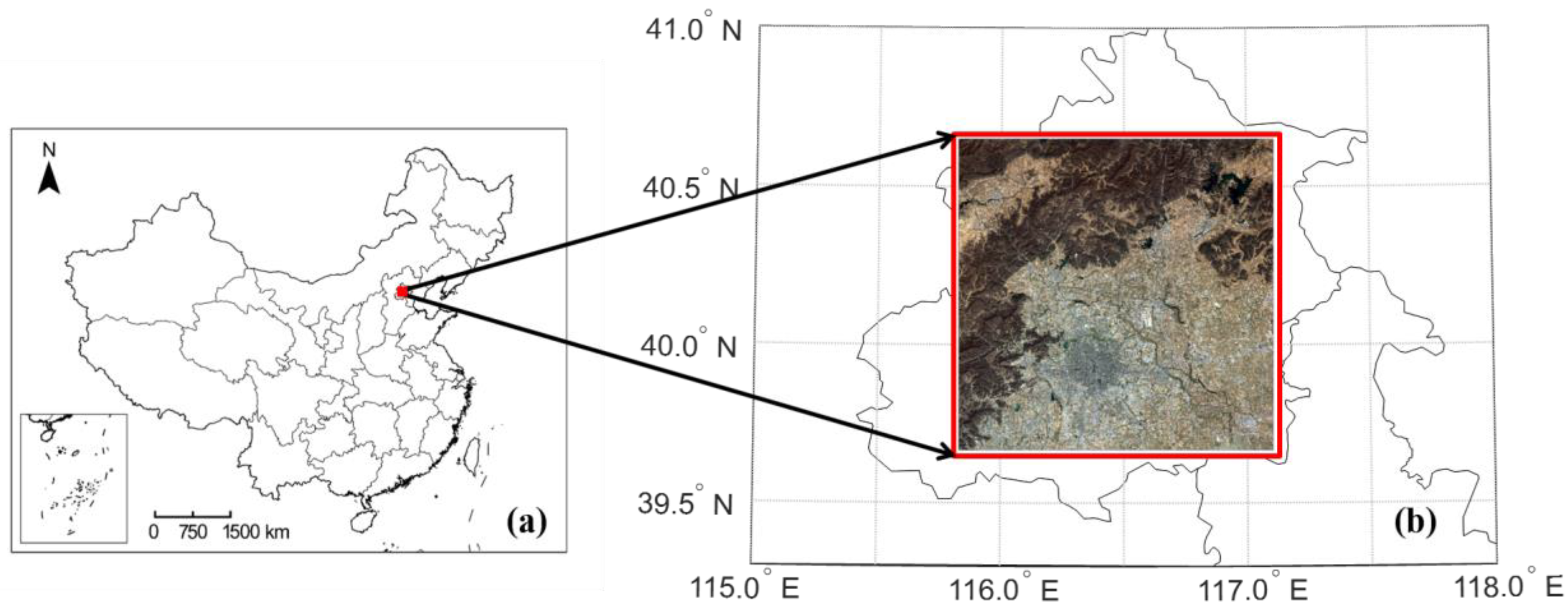
2.1. Study Area
The study area is a region covered by a scene of Sentinel-2 (Tile Number: T50TMK; central coordinate: 40°09′18.14″ N, 116°28′11.93″ E) in the north of China (Figure 1). This area covers the city of Beijing, the capital of China, and its surrounding rural area. Beijing is one of the most densely populated cities in the world with a population of 21.71 million. The total size of the study area is 109.8 km×109.8 km. The annual average air temperature and precipitation in this study area are approximately 11.5 °C and 610 mm respectively. This study area is located in the continental monsoon climatic zone with obvious seasonal alternation, and the main vegetation type is temperate deciduous broad-leaved forests. It has both a natural and a highly modernized urban ecosystem and has clear boundaries between the urban and rural areas. Based on a previous study [25], Beijing has significant rural-urban difference in vegetation spring phenology and this study area does not have persistent clouds year-round so that enough cloud-free satellite observations could be obtained to extract the phenology variables.
2.2. Data Used
Three types of satellite data in 2016 were used in this study: (1) Sentinel-2 L1C images (10 m), (2) Landsat-8 OLI images (30 m), and (3) NPP VIIRS nighttime light data (about 500 m). The Sentinel-2 and Landsat-8 images are fused to generate the time series at a spatial resolution of 10 m, and the NPP VIIRS nighttime light data is used to obtain the boundary that divides urban and rural areas. All Landsat-8 and Sentinel-2 images used in this study are summarized in Table 2. Details of each dataset are introduced in the following sub-sessions.
Sentinel-2 that consists of two twin satellites, provides multi-spectral images with spatial resolution from 10 m to 60 m and temporal resolution of 5 days. The onboard Multi-Spectral Instrument (MSI) can collect 13 spectral bands including four bands (BLUE, GREEN, RED and Near Infrared) at 10 m; 6 bands (vegetation RED Edges and SWIR) at 20 m for vegetation classification and snow, ice and cloud discrimination; and 3 bands (0.443, 0.945 and 1.375 μm) at 60 m for aerosol detection, water vapor and cirrus monitoring. In this study, Sentinel-2 L1C images (Tile Number: T50TMK) in 2016 were downloaded via USGS Earth Explorer (https://earthexplorer.usgs.gov/). This dataset has been geometrically corrected and converted to top of atmosphere (TOA) radiance [36].
Landsat-8 OLI collects eight spectral bands (Coastal Aerosol, BLUE, GREEN, RED, Near Infrared, SWIR-1, SWIR-1, and Cirrus) at 30 m [37]. In this study, nine Landsat-8 OLI surface reflectance images (Path: 123, Row: 032) in 2016 with cloud cover lower than 60% were collected via USGS Earth Explorer (http://earthexplorer.usgs.gov/). These images can cover the entire Sentinel-2 scene (Tile Number: T50TMK). Landsat-8 images with a spatial resolution of 30 m are fused with Sentinel-2 images (10 m) by the spatiotemporal data fusion algorithm [38].
Monthly composites of the daily Day/ Night Band (DNB) imagery of the Visible Infrared Imaging Radiometer Suite (VIIRS) onboard Suomi National Polar-orbiting Partnership (NPP) satellite provide reliable nighttime light data in 15 arc-second geographic grids (about 500 m). According to the location of our study area, the Tile 3 (75N060E) of NPP VIIRS nighttime light data in 2016 was collected from the Earth Observations Group (EOG) at NOAA/NCEI (https://ngdc.noaa.gov). Previous studies have demonstrated the high accuracy and good performance of this nighttime light dataset for extracting rural–urban boundaries [24,39].
3. Methods
3.1. Data Preprocessing
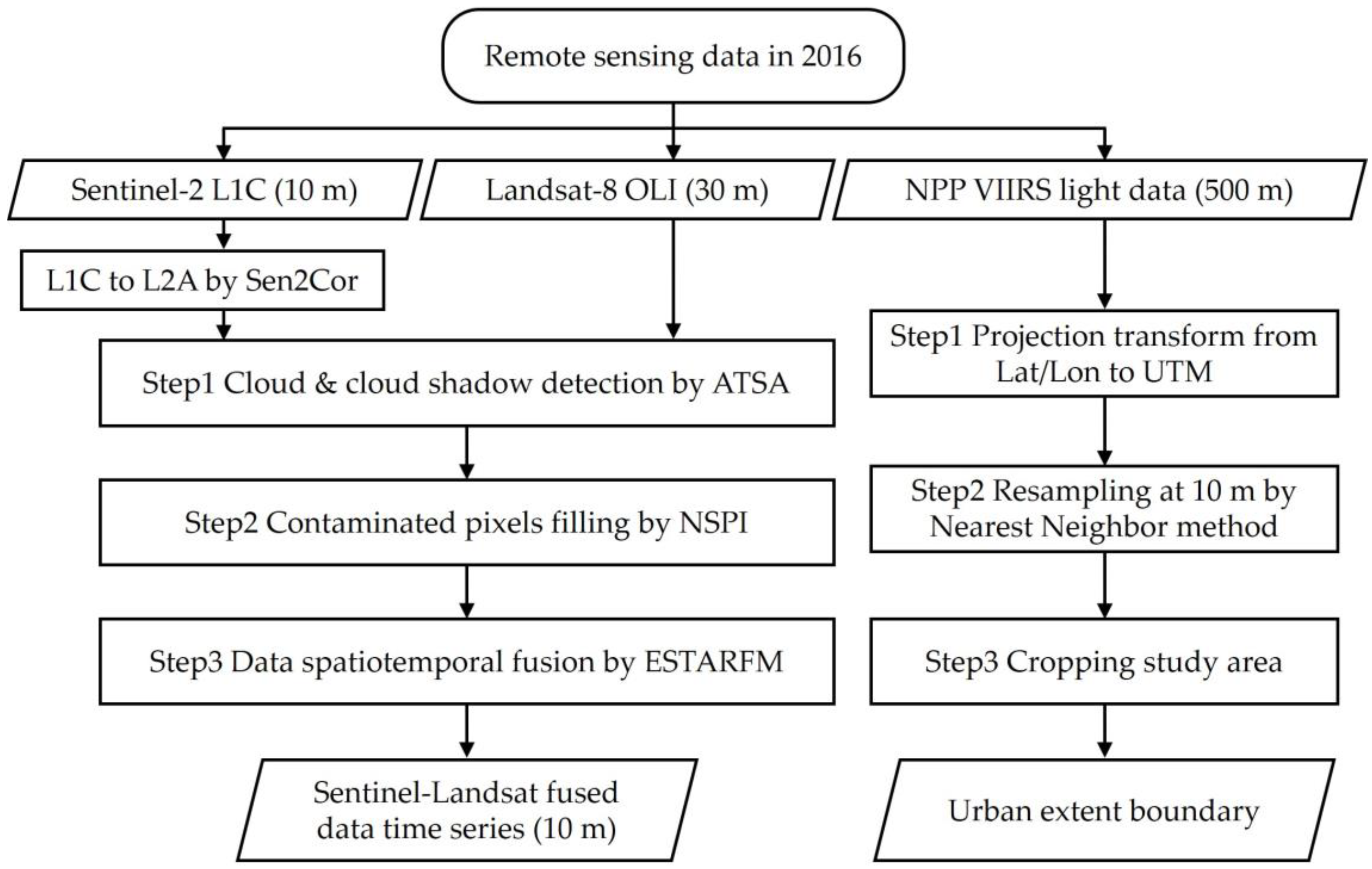
As Figure 2 shows, data preprocessing includes two streams: processing Sentinel-2 LIC images and Landsat-8 surface reflectance products to generate fused time series with a spatial resolution of 10 m, and processing NPP VIIRS nighttime light data to define the boundary of urban and rural areas.
3.1.1. Processing Sentinel-2 and Landsat-8 Images
First, the Sentinel-2 L1C images were TOA radiance, so they were further calibrated to surface reflectance by an official software Sen2Cor (http://step.esa.int/main/third-party-plugins-2/sen2cor/) to remove atmospheric effects. After that, three steps needed to be implemented to generate the high-quality time series at 10 m. In step 1, the Automatic Time-Series Analysis (ATSA) algorithm [40] was used to mask pixels of cloud and cloud shadow in Landsat-8 time series and Sentinel-2 time series respectively (see an example in Figure 3b). Based on the ATSA masks, manual inspection was executed to correct both omission and commission errors (Figure 3c). In step 2, those pixels contaminated by cloud and cloud shadows were filled by the neighborhood similar pixel interpolator (NSPI) method (Figure 3d), a promising interpolation method using spatial and temporal information of adjacent pixels with similar characteristics [41,42]. In step 3, Landsat-8 OLI and Sentinel-2 L2A images, after implementation of step 1 and step 2, were fused by the enhanced spatial and temporal adaptive reflectance fusion model (ESTARFM) (Figure 3e), a spatiotemporal fusion algorithm which improved the classic data fusion method STARFM [43,44] for heterogeneous landscapes [38]. From the zoom-in sub-image in Figure 3f,g, we can see that the spatial resolution of the Landsat image was improved after data fusion. In the end, a high-quality Sentinel-like time series at 10 m is generated.
3.1.2. Processing NPP VIIRS Nighttime Light Data
A smooth urban boundary is needed to quantify the urbanization effects on vegetation phenology. Previous studies of urbanization effects on vegetation phenology used nighttime light data to extract the urban boundary because it is closely related to human activities [24,45]. Compared to the urban extent extracted from the classification of daytime satellite images, the usage of nighttime images has several advantages: (1) it is more directly linked to the intensity of urbanization, (2) it is not affected by the classification errors of artificial surfaces, which are easily confused with bare soil and rocks, and (3) it can capture a smooth and meaningful rural–urban boundary. In this study, monthly NPP VIIRS nighttime light data were averaged to obtain the annual nighttime light over the study area in 2016. The urban boundary will be extracted from this annual nighttime light data. It should be noted that the extracted urban boundary has 500 m resolution, but it will be resampled to other resolutions for computing the rural–urban phenology difference at other scales. Given the large size of Beijing city and surrounding rural areas, a resampled urban boundary will not lead to large errors in the calculation of rural–urban phenology difference.
3.2. Generate NDVI Profiles at Different Spatial Resolutions
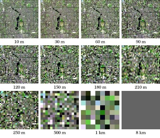
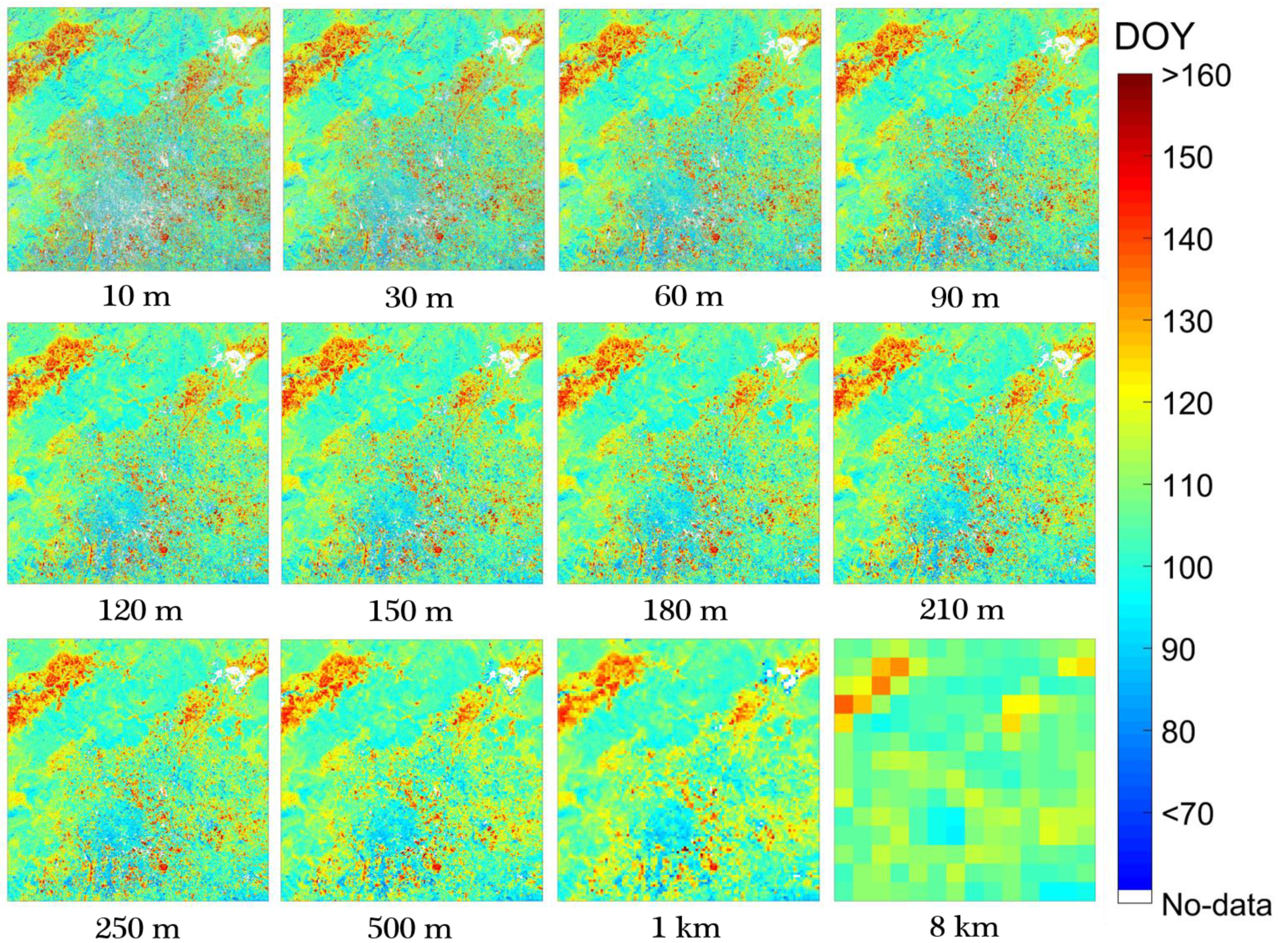
Satellite image time series at different spatial resolutions (i.e., from 30 m to 8 km) are needed to conduct this study. Although several satellite sensors, such as MODIS, SPOT-VGT, and AVHRR, provide NDVI products at different spatial resolutions, they are not sufficient to conduct a comprehensive study. This is due to these available products providing limited spatial resolutions, such as MODIS 250 m, SPOT-VGT and AVHRR 1 km and different sensors having differences in other aspects besides spatial resolution, such as, sensor configurations, dates of data acquisition, and atmospheric condition, which will make it harder to explore the effect of spatial resolution exclusively. Therefore, image time series with different spatial resolutions, including 30 m, 60 m, 90 m, 120 m, 150 m, 180 m, 210 m, 250 m, 500 m, 1 km, and 8 km, were simulated from the 10 m time series by the Pixel Aggregate method. To be specific, a pixel value at 30 m is generated by averaging the values of 3×3 pixels at 10 m. Figure 4 shows the appearance of an 8×8 km2 sub-region in images with different spatial resolutions from 10 m to 8 km. The Pixel Aggregate method is a widely used strategy to explore the scale effect of remote sensing data on land surface monitoring; for example, surface temperature [46], land cover characterization [47], and land change [48]. After generating image time series to other spatial resolutions from the original 10 m time series, NDVI profiles at each spatial resolution were calculated by Equation (1):
where NIR and RED mean the surface reflectance of NIR and RED bands, respectively.
NDVI = (NIR – RED)/(NIR + RED),
3.3. Extract Vegetation Spring Phenology
TIMESAT, a software package, was developed to extract pixel-based vegetation phenological metrics (e.g., start of season, end of season, growth length, and amplitude) from time series of vegetation indices (e.g., NDVI and EVI) [49,50]. Generally, TIMESAT includes two steps for extracting phenology, that is, data smoothing and extraction of phenological parameters. The former includes three fundamental smoothing approaches, adaptive Savizky-Golay (SG), asymmetric Gaussian and double logistic filtering, while the latter has two typical approaches, absolute threshold based and seasonal amplitude based [51].
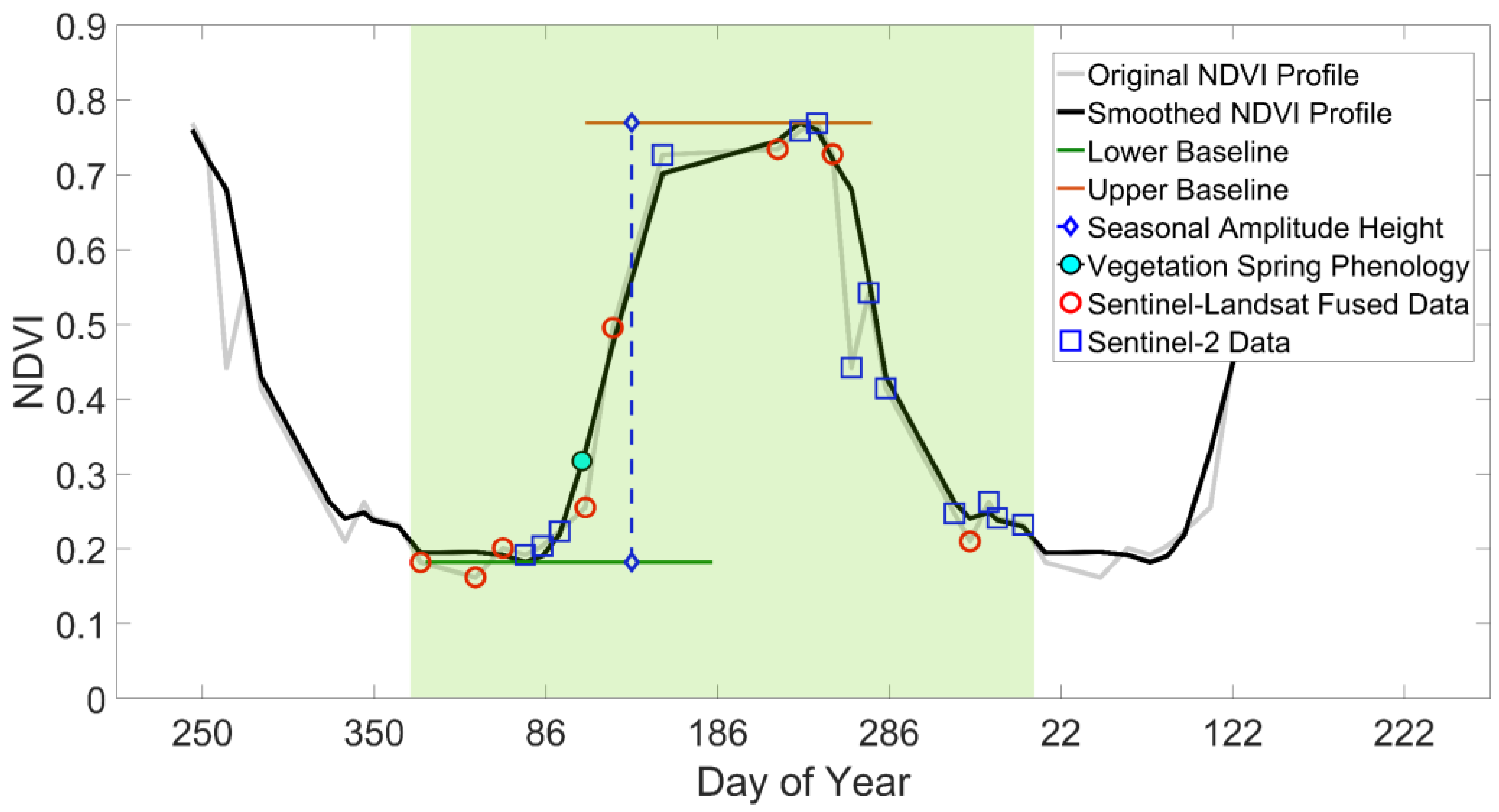
In this study, adaptive SG filtering and seasonal amplitude methods were used. Adaptive SG filtering was used to smooth the NDVI curves because it can obtain smoothed NDVI profiles that match ground measurements satisfactorily [52], and it is an effective smoothing method for preserving key features of the NDVI profile (e.g., relative maximum, minimum, and width of data) [53]. The seasonal amplitude method defines spring phenology as the time for which the NDVI increases to a user defined level (i.e., a certain fraction of the seasonal amplitude) measured from the left minimum level. It is a widely accepted method for extracting vegetation phenology in heterogeneous landscapes where pixels have diverse seasonal amplitudes. Based on previous studies [23,25], a threshold of 0.3 was used by this study to define vegetation spring phenology. Also, this study only extracts phenology from 1-year NDVI time series in 2016, so following the TIMESAT’s instruction, the 1-year NDVI time series was duplicated to make an artificial time series spanning 3 years run the TIMESAT software [51]. The principle of using TIMESAT to extract vegetation spring phenology is described in Figure 5, where the light-green region refers to the 1-year span of the NDVI profile in 2016. Following previous studies in temperate regions of the northern hemisphere [54,55,56], to reduce the uncertainties in phenology extraction in a complex urban area, pixels with a start of season earlier than the 60th or later than 160th day of the year are excluded in the further analysis.
3.4. Quantify Urbanization Effects
Existing studies quantify the urbanization effects on vegetation spring phenology as the difference of the average vegetation spring phenology between urbanized and rural areas as shown in Equation (2) [24,25].
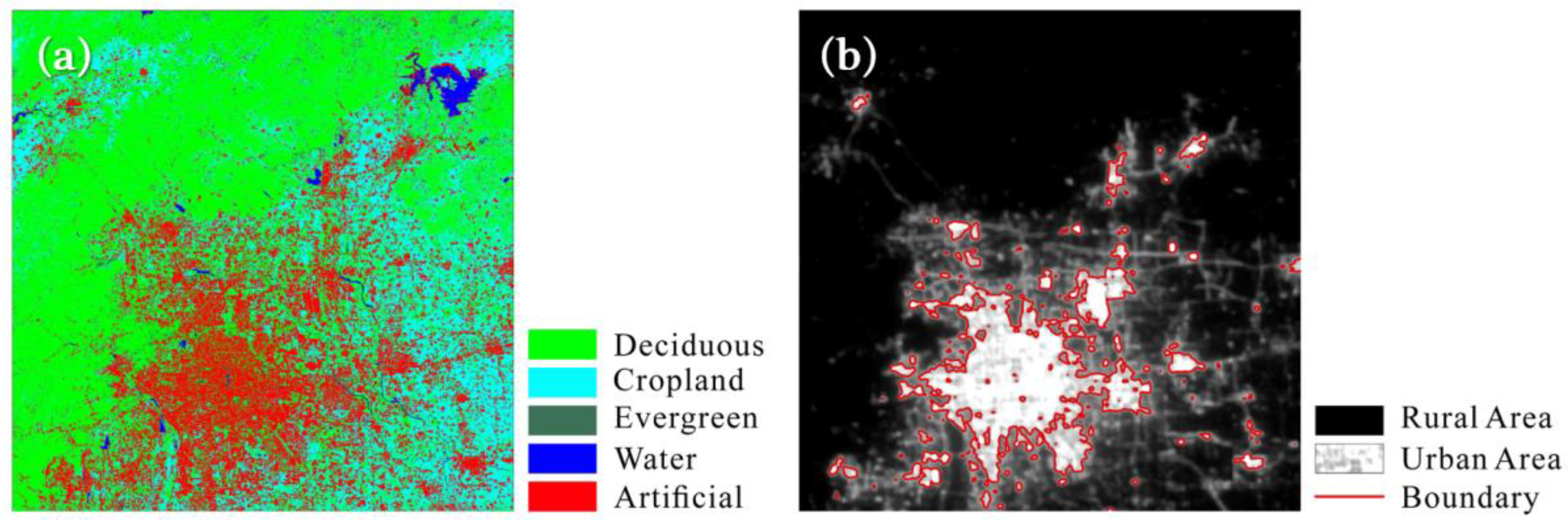
where AVSP means average vegetation spring phenology, and D indicates the rural–urban average difference, that is, urbanization effects on vegetation spring phenology. Considering only pixels of deciduous forests have clear growing cycles and their phenology is not manipulated by human activity, the other vegetation types (e.g., crops and evergreen forests) have been excluded when computing the urbanization effects using Equation (2) [29,33]. Accordingly, a deciduous forest mask and a rural-urban boundary mask need to be generated for calculating urbanization effects by Equation (2). First, according to the high-resolution images in Google Earth, we manually inspected and collected evenly-distributed training samples into five major land cover types, deciduous forests (2622 pixels), mainly focusing on parks, streets and rural deciduous pixels, evergreen forests (76 pixels), water (1106 pixels), cropland (2382 pixels), and artificial surfaces (1621 pixels). Afterwards, multi-temporal Sentinel-2 images (10 m) classified these five land types, as shown in Figure 6a, by the support vector machine (SVM) method with better performance of land cover classification [57]. The proportions of these five classes are deciduous forests (48.2%), evergreen forests (1.5%), water (1.2%), cropland (26.1%), and artificial surfaces (23.0%). To acquire a purer deciduous mask, the pixels satisfying the following three criteria were used: (1) the average NDVI during June to September is greater than 0.10 [58] to ensure that substantial vegetation exists in the pixel, (2) the average NDVI from July to September is higher than 1.2 times the average NDVI during November to March [59] to ensure that vegetation has significant seasonality, and (3) RMSE between the original NDVI profile and smoothed NDVI should be lower than 0.08, which is validated by ground observations [52] to ensure that the original NDVI profile is not too noisy.
D = AVSPrural – AVSPurban,
The rural–urban boundary mask was generated by the NPP VIIRS nighttime light image. An optimal threshold of nighttime light should well separate the built-up area of Beijing and the surrounding croplands. To search for the optimal thresholds, we calculated the proportions of croplands and built-up area included in the urban area defined by different thresholds in the NPP VIIRS nighttime light image. In this way, the nighttime image pixel value 15 was selected as the optimal threshold for generating the rural–urban boundary as shown in Figure 6b. Additionally, the isolated small urbanized patches that are distant from the major urban area were excluded. To match vegetation spring phenological results at each spatial scale, the deciduous forest mask and urban extent mask are resampled to 30 m to 8 km by the Pixel Aggregate method. Specifically, in the aggregated coarse pixel, if the fraction of deciduous forests is larger than 0, this coarse pixel is regarded as deciduous forests. In addition, to avoid the impact of cropland on the spring vegetation detection of coarse pixels [33], those coarse deciduous forest pixels will be excludes if their fraction of cropland is larger than 0.05.
4. Results and Discussion
4.1. Urbanization Effects on Vegetation Spring Phenology at Different Spatial Resolutions
The spatial distributions of spring phenology of all vegetation types (including deciduous trees and crops) extracted by seasonal amplitude method (threshold: 0.3) in TIMESAT software from images with different spatial resolutions are shown in Figure 7. Seasonal amplitude method (also known as relative threshold method) to extract vegetation phenology is widely used, and it has been validated by ground truth and another phenological extraction method (e.g., inflexion-based method) [59,60,61]. Moreover, the parameter (0.3) is an empirical threshold that is more suitable for phenology monitoring in the north of China according to the previous studies [23]. A further robustness test of applied methods and thresholds was explored in the Section 4.3. The range of color bars of Figure 7 was unified for each figure. It is apparent that vegetation spring phenology in the central regions (urban areas) is earlier than surrounding regions (rural areas) at all spatial resolutions. Also, compared with the land cover map in Figure 6a, the regions of late spring phenology in Figure 7 are mainly cropland, because the spring phenology of the major crops in Beijing is significantly later than natural deciduous forests. This confirms the necessity of excluding croplands to accurately quantify urbanization effects on vegetation spring phenology at different spatial resolutions. Otherwise, the late vegetation spring phenology of cropland would lead to a large overestimation of the rural–urban phenology difference.
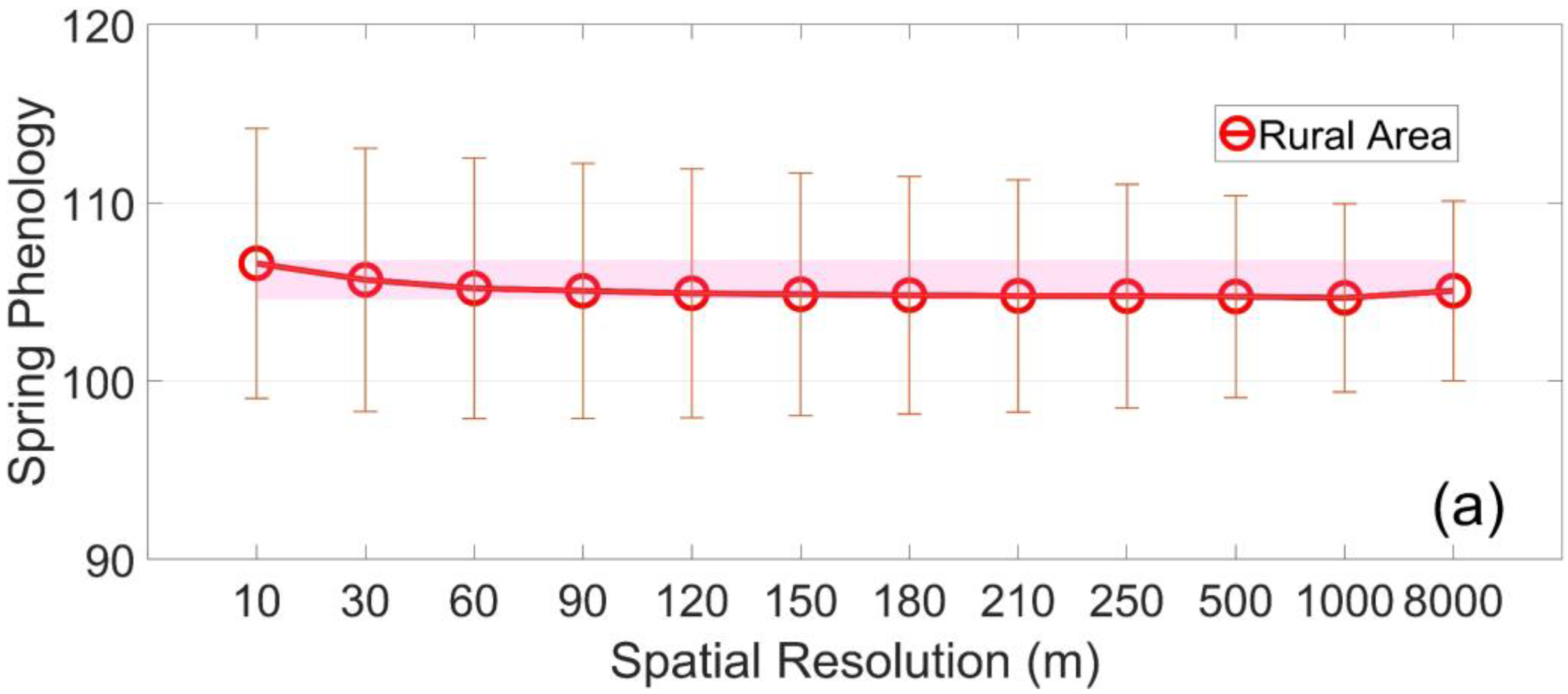
The vegetation spring phenology (i.e., deciduous forests) in urban and rural areas at different spatial resolutions is quantified and summarized in Figure 8. It shows that vegetation spring phenology in urban areas is earlier than rural areas regardless of spatial resolution, and the extracted spring phenology in both rural and urban areas is earlier at coarser resolution (hereafter named as “earlier-shifting”) but the magnitude of this earlier-shifting is different between rural and urban areas. Specifically, the vegetation spring phenology in rural areas from 10 m to 8 km is relatively stable (from 107 to 105 DOY, the pink range in Figure 8a), whereas the spring phenology in urban areas shifts to the much earlier dates with coarse spatial resolutions (from 105 to 97 DOY, the blue range in Figure 8b). The earlier-shifting pattern has a breakpoint at 90 m in urban areas. When spatial resolutions are finer than 90 m (e.g., 10 m, 30 m and 60 m), the earlier-shifting trend is sharp while the trend becomes flat at spatial resolutions coarser than 90 m (e.g., 120 m to 8 km), as shown in Figure 8b.
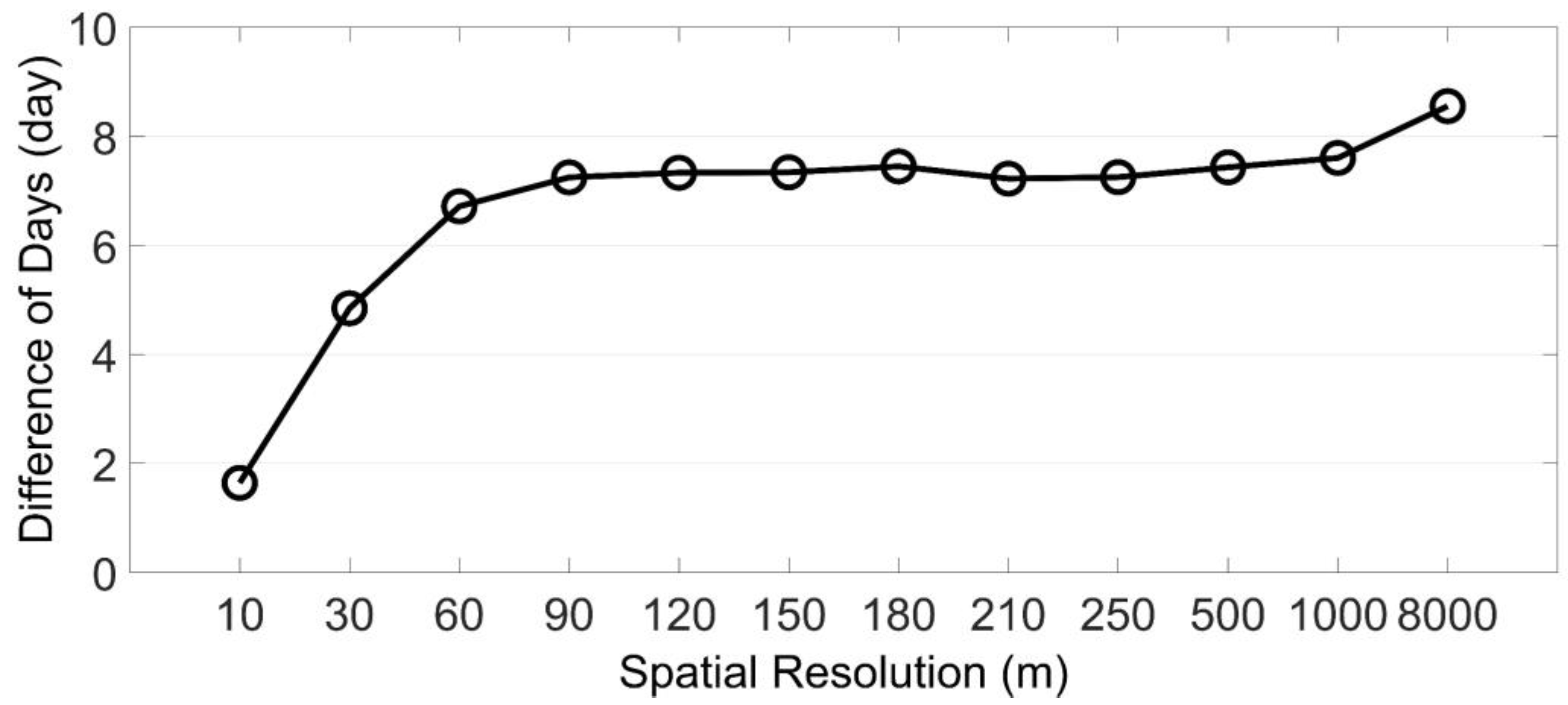
The quantitative result of urbanization effects, that is, the vegetation spring phenological average difference between rural and urban areas at each spatial resolution, is shown in Figure 9. It is reasonable to assume that the urbanization effect at 10 m is the most accurate result because most vegetation pixels are more likely dominated by the same species. It is clear that the urbanization effects show an evident overestimation from 10 m to 8 km spatial resolutions, and this overestimation trend can be divided into two segments, a sharp increase from 10 m to 90 m, and a stable overestimate from 90 m to 8 km.
4.2. Possible Reasons for the Amplified Urbanization Effects at Coarse Spatial Resolutions
Urbanization effects on vegetation spring phenology were explored widely, as shown in Table 1. Although existing studies were carried out in various areas, employed different phenological extraction algorithms, and used satellite data with a wide range of spatial scales (30 m to 1 km), they came to a similar conclusion: vegetation spring phenology in urban areas is earlier than rural areas because of the change of natural environment (e.g., increase of temperature and artificial light). This conclusion has been thoroughly validated by satellite-based remotely sensed data and ground observations [2,23,26,32,62]. Our study also confirmed this conclusion. Moreover, the current study demonstrated that vegetation spring phenology in urban areas is always earlier than rural areas observed from satellite images using a range of spatial resolutions (Figure 8). In addition, we found that vegetation spring phenology in rural areas remains relatively stable cross different resolutions, but in urban areas, predictions of phenology vary significantly between 10 m and 8 km spatial resolutions (Figure 8), which leads to the amplified urbanization effects at coarse spatial resolutions (Figure 9).
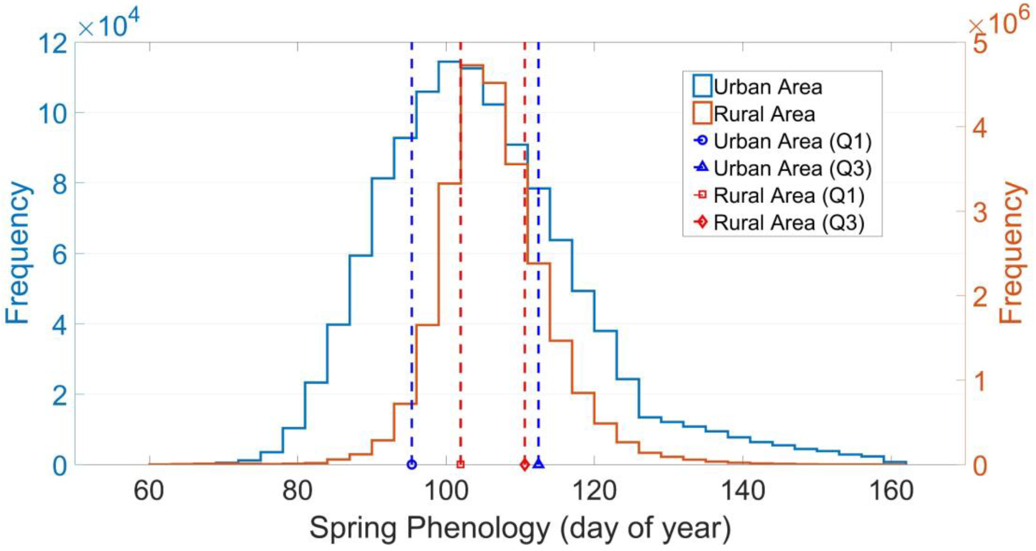
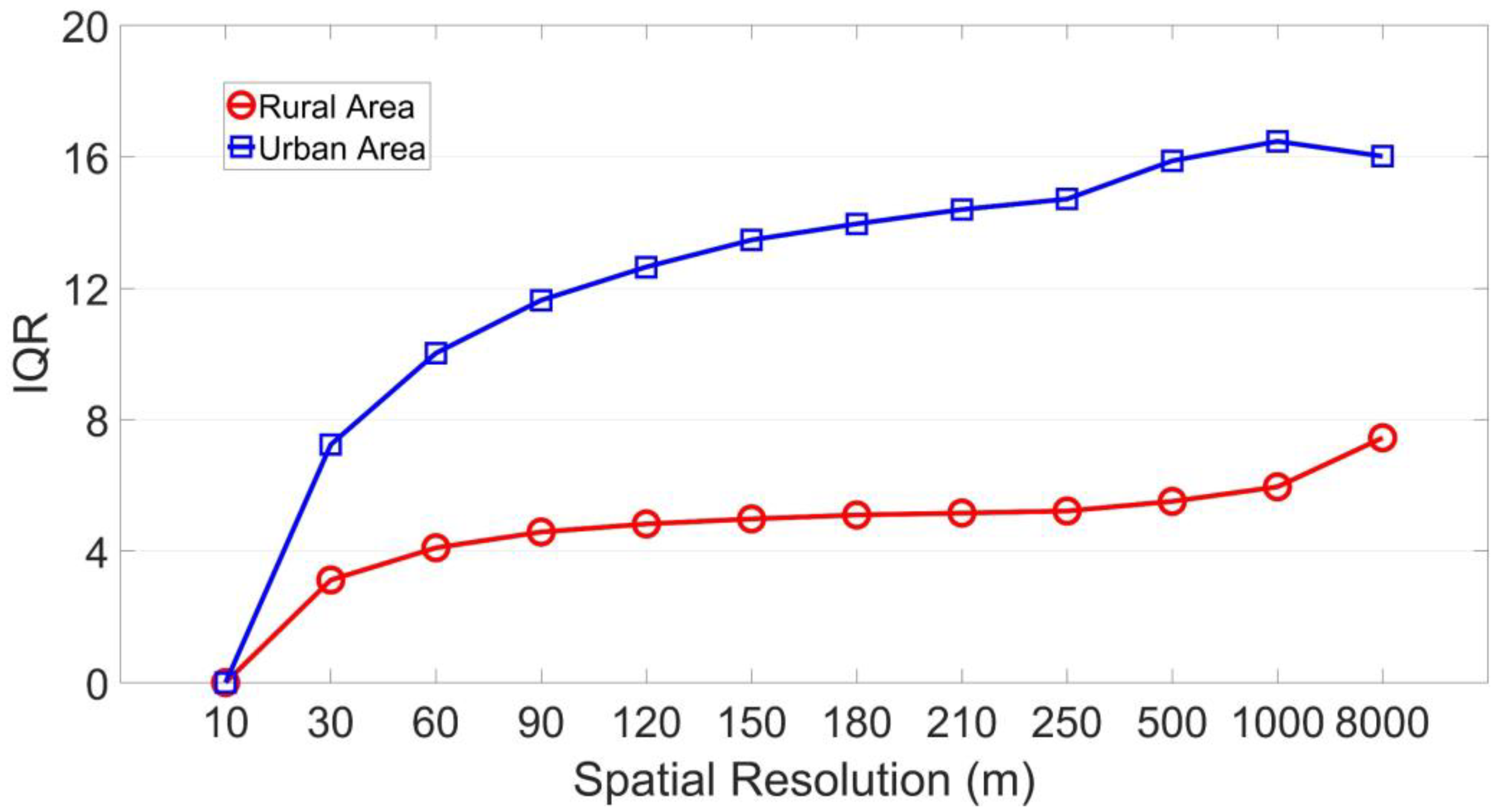
To explore the reasons underlying the amplified urbanization effects at coarse spatial resolution, we further employed a histogram of vegetation spring phenology at a spatial resolution of 10 m in both urban and rural areas (Figure 10), which are regarded as the “pure” vegetation pixels. We found that vegetation spring phenology in urban areas has higher diversity, earlier spring phenology at first quartile (Q1), and later spring phenology at third quartile (Q3) than rural areas, as shown in Figure 10. This is mainly due to both the natural environment and vegetation species being relatively uniform in rural areas. However, they are much more complicated and heterogeneous in urban areas due to human activities (i.e., artificial light, ground water, land cover types, and planted vegetation), which results in the greater difference of vegetation spring phenology. Then, we calculated average Interquartile Range (IQR) at spatial resolutions from 10 m to 8 km in rural and urban areas to analyze mixed situations of spring phenology at each spatial resolution (Figure 11). As expected, Figure 11 shows that both IQR in rural and urban areas have increasing trends along with spatial resolutions, which means that the diversity of spring phenology of pixels becomes greater when mixing into coarse pixels. This is opposite to the variation of vegetation spring phenology with spatial resolution (Figure 8). To be specific, the IQR in rural areas is relatively stable at each spatial resolution while the urban IQR experiences a significant increase from IQR 0 day of “pure” vegetation at 10 m resolution to IQR 16 days at 8 km resolution. Additionally, the IQR in the urban area increases greatly from 10 m to 90 m and becomes more stable (12–16 days) at spatial resolutions coarser than 90 m. When we compared results displayed in Figure 11 with the spring phenology extracted from images of different spatial resolutions in Figure 8, it is clear that spring phenology in both rural and urban areas has a negative correlation with the IQR (correlation coefficients: rural: -0.877, urban: -0.969), suggesting that the large within-pixel diversity of spring phenology (i.e., large IQR) leads to earlier spring phenology detected from satellite images. Our results are thus well-aligned with current studies which found that species with earlier spring phenology in a mixed pixel results in earlier detections of phenological changes than ground truth observations [33,63].
As documented, a simulation experiment [33] suggested that the compositions of vegetation species with different spring phenological dates in mixed pixels lead to the uncertainty of vegetation spring phenology extraction. In addition, two recent studies indicated that spring phenology of a coarse pixel is prone to be closer to that of a fine pixel with earlier spring phenology and higher vegetation growth speed [35,63]. Therefore, we assume that the overestimated urbanization effects at coarse spatial resolutions is mainly due to the amplified heterogeneity of vegetation spring phenology of mixed pixels at coarser spatial resolutions, especially in urban areas. Specifically, compared with rural areas, urban areas have higher diversity in terms of spring phenology as deciduous trees in urban areas mainly consist of planted trees with different growth conditions and are located in different environments, for example, street trees and garden trees. Thus, with spatial resolution getting coarser, spring phenology in rural areas remains stable whereas urban vegetation spring phenology shifts to earlier dates, which results in the overestimation of urbanization effects on spring phenology.
4.3. Simulation Experiments
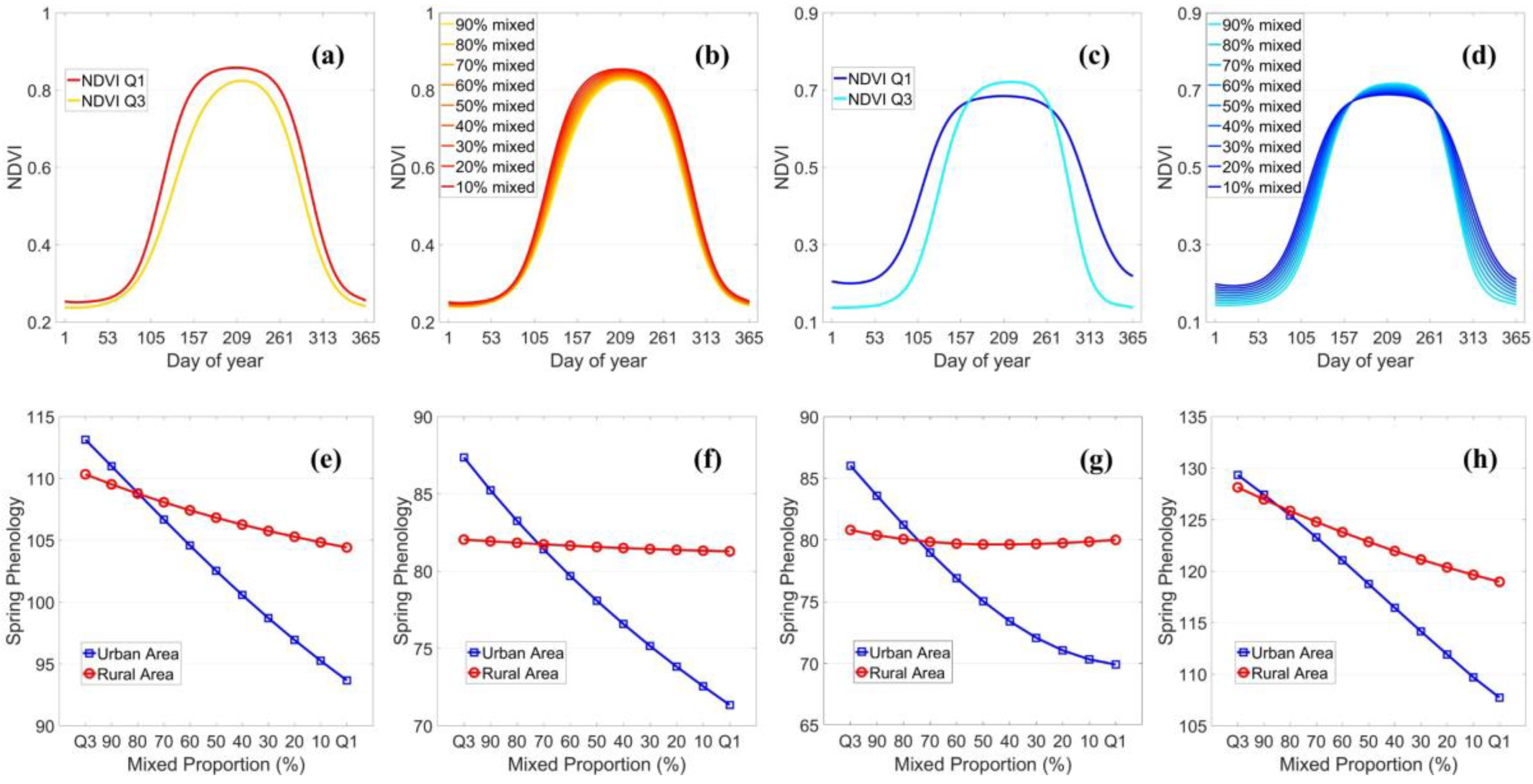
To further confirm whether spatial resolutions of satellite images can cause misestimation of vegetation spring phenology, a simulation experiment was conducted using the Land Surface Phenology Simulation software [33] to examine the spring phenology detected from pixels with varying degrees of mixture between two vegetation endmembers. First, we simulated NDVI profiles of mixed pixels though the linear combination of two vegetation endmembers (i.e., vegetation pixel with spring phenological dates of the first quartile Q1 and third quartile Q3 in urban and rural areas respectively) and with varying degrees of mixture (from non-mixed to 90% mixed) as shown in Figure 12 in rural and urban areas. For instance, the 10% mixed means that the simulated NDVI profile contains 90% Q1 NDVI profile and 10% Q3 NDVI profile. After that, several widely used methods and thresholds, i.e., seasonal amplitude (as known as relative threshold method) with thresholds of 0.1 and 0.3, inflexion-based method and midpoint method, were used to extract vegetation spring phenology of these simulated mixed NDVI profiles.
Figure 12 shows spring phenological dates extracted from the simulated mixed pixels. It reveals that vegetation spring phenology detected from NDVI time series becomes earlier when the mixed pixels have more proportions of NDVI Q1 with earlier spring phenology. Moreover, compared with rural areas, the earlier shifting of spring phenology in urban areas is stronger with mixed proportions (Figure 12e,f,g,h). This simulation experiment confirmed that the amplified urbanization effects on spring phenology shown in Figure 9 is the result of vegetation mixture in coarse pixels. Additionally, the simulation experiment shows that change in vegetation spring phenology is marginal when mixing two rural NDVI profiles with similar spring phenology dates (the change is around 5 days), as the red line shows in Figure 12e. However, the change of vegetation spring phenology was sharp when two urban NDVI profiles were mixed. For example, the detected spring phenology date of the simulated mixed NDVI profile is around 20 days earlier when the vegetation proportion decreases from pure to 90% mixed, as the blue line shows in Figure 12e. In addition, other simulated results extracted by different approaches and parameters show a similar conclusion, that is, mixed spring phenology in urban areas has more significant changes than rural areas (Figure 12f,g,h), which reflects the strong robustness of the seasonal amplitude method used to export spring phenology in this study. Moreover, according to a previous study [59], spatial patterns of deciduous forest spring phenology extracted by five different methods are highly similar. Similarly, a recent study [33] also validated that the results of deciduous forest spring phenology extraction for mixed pixels have very high consistency using relative threshold and inflexion-based methods.
4.4. Limitations
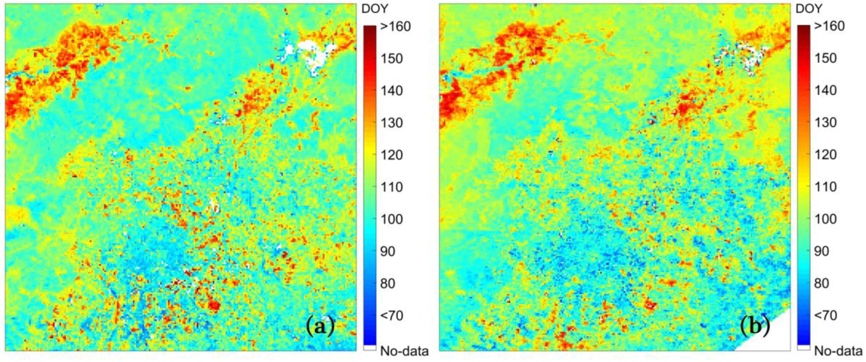
This study has several limitations. First, the images with different spatial resolutions were stimulated from the 10 m data sets which may be different from the real satellite images. Currently, data from different spatial resolutions are limited, so simulation images enabled us to explore images with abundant spatial resolutions. Another benefit of using simulated images is to reduce the influence of atmospheric conditions and sensor configurations from different satellites when comparing their results, so that we can solely evaluate the impact of spatial resolutions on the results. However, the phenology detected from simulated images may be different from real satellite images which would affect practical values of findings from simulated images. To evaluate this problem, we compared vegetation spring phenology extracted from two datasets, simulated 500 m NDVI time series and real 500 m MODIS NDVI time series in 2016 (MOD13A1 product downloaded from USGS: https://earthexplorer.usgs.gov/). To cover our study area, two MODIS Tiles (h26v04 and h26v05) were mosaicked. Afterwards, we used the same method and same parameters (SG filtering and seasonal relative threshold of 0.3) in TIMESAT to extract vegetation spring phenology of MODIS NDVI profiles. The result shows that the patterns of vegetation spring phenology between a simulated image (500 m) and MODIS (500 m) are coincident (Figure 13). Additionally, the urbanization effect assessed by real MODIS images is around 9 days, which is similar with results from the resampled Sentinel-Landsat time series (7.4 days). Both results show a more significant urbanization effect at 500 m than finer spatial resolutions (e.g., 10 m).
Second, the rural–urban phenology difference at 10 m was used as a reference to judge the results at other spatial resolutions. It should be noted that 10 m may not be high enough for detecting urban vegetation phenology considering the high heterogeneity of the urban landscape. To more accurately assess the urban effect on vegetation phenology, satellite time-series data with spatial resolution within 10 m are needed. Fortunately, it is expected that such data sets will be available soon due to the fast development of small satellites and satellite constellations.
Third, Beijing and surrounding rural areas were used as a pilot area in this study. These data might not be sufficient to comprehensively evaluate the influence of spatial resolution on vegetation spring phenology in an urban environment. Our main objective of this study was to answer an important technical question, i.e., how spatial resolution of satellite images affects the results of rural–urban difference in vegetation spring phenology rather than studying urbanization effects on vegetation spring phenology in many cities. Our study provides a prototype for investigating this scale issue and may improve awareness on scale issues when using satellite data to assess urbanization effects on vegetation phenology. Future studies in more cities can help to thoroughly explore this issue.
5. Conclusion
It is not well known whether satellite-based time series with coarse resolutions can accurately detect urbanization effects on vegetation spring phenology. This study fills this research gap. In light of our results, we found that the difference between vegetation spring phenology in rural and urban at different spatial resolutions are not coincident, and specifically, the rural–urban difference is amplified with coarser spatial resolutions. A possible reason for this inconsistency is that coarse images tend to have more mixed pixels with higher diversity in terms of spring phenology dates, which leads to the detected vegetation spring phenology being earlier than the real situation.
We suggest that future studies that explore the urban vegetation phenology use satellite images with a spatial resolution as high as possible. According to the findings of our study, it is better to use satellite images in which most vegetation pixels are “pure” to reduce the uncertainty in spring phenology detection. Specifically, in cities like Beijing, satellite images with spatial resolution finer than 30 m are superior when exploring urbanization effects on vegetation spring phenology. However, current available satellite-based vegetation index time series cannot be compatible with high temporal and high spatial resolution. Recently, a fused dataset, Harmonized Landsat-8 Sentinel-2 (HLS) product with 5-day and 30 m spatial resolution, was used directly for studying urbanization effects on vegetation phenology, but the spatial coverage was limited at this time. Alternatively, we can fuse data from multiple satellites by various spatiotemporal data fusion algorithms. This study also provides a detailed procedure to generate high-quality time series by fusing images from two satellites (i.e., Sentinel-2 and Landsat-8) that can be adopted in future studies.
Author Contributions
Conceptualization, J.T., X.Z. and J.C.; Methodology, J.T. and X.Z.; Software, J.T.; Validation, J.T.; Formal Analysis, J.T. and X.Z.; Investigation, J.T.; Resources, J.T.; Data Curation, J.T.; Writing-Original Draft Preparation, J.T.; Writing-Review & Editing, X.Z., J.W., M.S. and J.C.; Visualization, J.T.; Supervision, X.Z.; Project Administration, X.Z.; Funding Acquisition, X.Z. All authors have read and agreed to the published version of the manuscript.
Funding
This study was funded by the National Natural Science Foundation of China (project no.41701378), Research Grants Council of Hong Kong (project no.25222717), and Research Institute for Sustainable Urban Development, the Hong Kong Polytechnic University (project no. 1-BBWD).
Acknowledgments
We thank Trecia Kay-Ann Williams for improving the quality of this paper.
Conflicts of Interest
The authors declare no conflict of interests. The founding sponsors had no role in the design of the study; in the collection, analyses, or interpretation of data; in the writing of the manuscript, and in the decision to publish the results.
References
- Shen, M.; Piao, S.; Chen, X.; An, S.; Fu, Y.H.; Wang, S.; Cong, N.; Janssens, I.A. Strong impacts of daily minimum temperature on the green-up date and summer greenness of the Tibetan Plateau. Glob. Chang. Biol. 2016, 22, 3057–3066. [Google Scholar] [CrossRef] [PubMed]
- Bennie, J.; Davies, T.W.; Cruse, D.; Gaston, K.J. Ecological effects of artificial light at night on wild plants. J. Ecol. 2016, 104, 611–620. [Google Scholar] [CrossRef] [Green Version]
- Fu, Y.H.; Piao, S.; Delpierre, N.; Hao, F.; Hänninen, H.; Liu, Y.; Sun, W.; Janssens, I.A.; Campioli, M. Larger temperature response of autumn leaf senescence than spring leaf-out phenology. Glob. Chang. Biol. 2018, 24, 2159–2168. [Google Scholar] [CrossRef] [PubMed]
- Shen, M.; Tang, Y.; Chen, J.; Yang, X.; Wang, C.; Cui, X.; Yang, Y.; Han, L.; Li, L.; Du, J.; et al. Earlier-Season Vegetation Has Greater Temperature Sensitivity of Spring Phenology in Northern Hemisphere. PLoS ONE 2014, 9. [Google Scholar] [CrossRef] [PubMed]
- Shen, M.; Piao, S.; Cong, N.; Zhang, G.; Jassens, I.A. Precipitation impacts on vegetation spring phenology on the Tibetan Plateau. Glob. Chang. Biol. 2015, 21, 3647–3656. [Google Scholar] [CrossRef] [Green Version]
- Fu, Y.H.; Zhao, H.; Piao, S.; Peaucelle, M.; Peng, S.; Zhou, G.; Ciais, P.; Huang, M.; Menzel, A.; Peñuelas, J.; et al. Declining global warming effects on the phenology of spring leaf unfolding. Nature 2015, 526, 104–107. [Google Scholar] [CrossRef] [Green Version]
- Richardson, A.D.; Hufkens, K.; Milliman, T.; Aubrecht, D.M.; Furze, M.E.; Nettles, R.; Heiderman, R.R.; Seyednasrollah, B.; Krassovski, M.B.; Latimer, J.M.; et al. Ecosystem warming extends vegetation activity but heightens vulnerability to cold temperatures. Nature 2018, 560, 368. [Google Scholar] [CrossRef]
- Brown, M.E.; de Beurs, K.M.; Marshall, M. Global phenological response to climate change in crop areas using satellite remote sensing of vegetation, humidity and temperature over 26 years. Remote Sens. Environ. 2012, 126, 174–183. [Google Scholar] [CrossRef]
- Yang, B.; He, M.; Shishov, V.; Tychkov, I.; Vaganov, E.; Rossi, S.; Ljungqvist, F.C.; Bräuning, A.; Grießinger, J. New perspective on spring vegetation phenology and global climate change based on Tibetan Plateau tree-ring data. Proc. Natl. Acad. Sci. USA 2017, 114, 6966–6971. [Google Scholar] [CrossRef] [Green Version]
- Shen, M.; Piao, S.; Dorji, T.; Liu, Q.; Cong, N.; Chen, X.; An, S.; Wang, S.; Wang, T.; Zhang, G. Plant phenological responses to climate change on the Tibetan Plateau: Research status and challenges. Nat. Sci. Rev. 2015, 2, 454–467. [Google Scholar] [CrossRef] [Green Version]
- Buitenwerf, R.; Rose, L.; Higgins, S.I. Three decades of multi-dimensional change in global leaf phenology. Nat. Clim. Chang. 2015, 5, 364–368. [Google Scholar] [CrossRef]
- Piao, S.; Cui, M.; Chen, A.; Wang, X.; Ciais, P.; Liu, J.; Tang, Y. Altitude and temperature dependence of change in the spring vegetation green-up date from 1982 to 2006 in the Qinghai-Xizang Plateau. Agric. For. Meteorol. 2011, 151, 1599–1608. [Google Scholar] [CrossRef]
- Shen, M.; Cao, R. Temperature sensitivity as an explanation of the latitudinal pattern of green-up date trend in Northern Hemisphere vegetation during 1982–2008. Int. J. Climatol. 2015, 35, 3707–3712. [Google Scholar] [CrossRef]
- Chen, M.; Melaas, E.K.; Gray, J.M.; Friedl, M.A.; Richardson, A.D. A new seasonal-deciduous spring phenology submodel in the Community Land Model 4.5: Impacts on carbon and water cycling under future climate scenarios. Glob. Chang. Biol. 2016, 22, 3675–3688. [Google Scholar] [CrossRef] [PubMed] [Green Version]
- Richardson, A.D.; Keenan, T.F.; Migliavacca, M.; Ryu, Y.; Sonnentag, O.; Toomey, M. Climate change, phenology, and phenological control of vegetation feedbacks to the climate system. Agric. For. Meteorol. 2013, 169, 156–173. [Google Scholar] [CrossRef]
- Han, Q.; Wang, T.; Jiang, Y.; Fischer, R.; Li, C. Phenological variation decreased carbon uptake in European forests during 1999–2013. For. Ecol. Manage. 2018, 427, 45–51. [Google Scholar] [CrossRef]
- Piao, S.; Fang, J.; Ciais, P.; Peylin, P.; Huang, Y.; Sitch, S.; Wang, T. The carbon balance of terrestrial ecosystems in China. Nature 2009, 458, 1009–1013. [Google Scholar] [CrossRef]
- Richardson, A.D.; Andy Black, T.; Ciais, P.; Delbart, N.; Friedl, M.A.; Gobron, N.; Hollinger, D.Y.; Kutsch, W.L.; Longdoz, B.; Luyssaert, S.; et al. Influence of spring and autumn phenological transitions on forest ecosystem productivity. Philos. Trans. R. Soc. B Biol. Sci. 2010, 365, 3227–3246. [Google Scholar] [CrossRef] [Green Version]
- Piao, S.; Ciais, P.; Friedlingstein, P.; Peylin, P.; Reichstein, M.; Luyssaert, S.; Margolis, H.; Fang, J.; Barr, A.; Chen, A.; et al. Net carbon dioxide losses of northern ecosystems in response to autumn warming. Nature 2008, 451, 49–52. [Google Scholar] [CrossRef]
- Keenan, T.F.; Gray, J.; Friedl, M.A.; Toomey, M.; Bohrer, G.; Hollinger, D.Y.; Munger, J.W.; O’Keefe, J.; Schmid, H.P.; Wing, I.S.; et al. Net carbon uptake has increased through warming-induced changes in temperate forest phenology. Nat. Clim. Chang. 2014, 4, 598–604. [Google Scholar] [CrossRef]
- Zipper, S.C.; Schatz, J.; Singh, A.; Kucharik, C.J.; Townsend, P.A.; Loheide, S.P., II. Urban heat island impacts on plant phenology: Intra-urban variability and response to land cover. Environ. Res. Lett. 2016, 11, 54023. [Google Scholar] [CrossRef]
- Parece, T.; Campbell, J. Intra-Urban Microclimate Effects on Phenology. Urban Sci. 2018, 2, 26. [Google Scholar] [CrossRef] [Green Version]
- Yao, R.; Wang, L.; Huang, X.; Guo, X.; Niu, Z.; Liu, H. Investigation of urbanization effects on land surface phenology in Northeast China during 2001-2015. Remote Sens. 2017, 9, 1–17. [Google Scholar] [CrossRef] [Green Version]
- Li, X.; Zhou, Y.; Asrar, G.R.; Mao, J.; Li, X.; Li, W. Response of vegetation phenology to urbanization in the conterminous United States. Glob. Chang. Biol. 2016, 23, 2818–2830. [Google Scholar] [CrossRef]
- Zhou, D.; Zhao, S.; Zhang, L.; Liu, S. Remotely sensed assessment of urbanization effects on vegetation phenology in China’s 32 major cities. Remote Sens. Environ. 2016, 176, 272–281. [Google Scholar] [CrossRef] [Green Version]
- Qiu, T.; Song, C.; Li, J. Impacts of urbanization on vegetation phenology over the past three decades in Shanghai, China. Remote Sens. 2017, 9, 1–16. [Google Scholar] [CrossRef] [Green Version]
- Han, G.; Xu, J. Land surface phenology and land surface temperature changes along an urban-rural gradient in yangtze River Delta, China. Environ. Manage. 2013, 52, 234–249. [Google Scholar] [CrossRef]
- Gervais, N.; Buyantuev, A.; Gao, F. Modeling the Effects of the Urban Built-Up Environment on Plant Phenology Using Fused Satellite Data. Remote Sens. 2017, 9, 99. [Google Scholar] [CrossRef] [Green Version]
- Zhang, X.; Friedl, M.A.; Schaaf, C.B.; Strahler, A.H.; Schneider, A. The footprint of urban climates on vegetation phenology. Geophys. Res. Lett. 2004, 31, 10–13. [Google Scholar] [CrossRef]
- Melaas, E.K.; Wang, J.A.; Miller, D.L.; Friedl, M.A. Interactions between urban vegetation and surface urban heat islands: A case study in the Boston metropolitan region. Environ. Res. Lett. 2016, 11. [Google Scholar] [CrossRef] [Green Version]
- Zhang, X.; Friedl, M.A.; Schaaf, C.B.; Strahler, A.H. Climate controls on vegetation phenological patterns in northern mid- and high latitudes inferred from MODIS data. Glob. Chang. Biol. 2004, 10, 1133–1145. [Google Scholar] [CrossRef]
- White, M.A.; Nemani, R.R.; Thornton, P.E.; Running, S.W. Satellite evidence of phenological differences between urbanized and rural areas of the eastern United States deciduous broadleaf forest. Ecosystems 2002, 5, 260–273. [Google Scholar] [CrossRef]
- Chen, X.; Wang, D.; Chen, J.; Wang, C.; Shen, M. The mixed pixel effect in land surface phenology: A simulation study. Remote Sens. Environ. 2018, 211, 338–344. [Google Scholar] [CrossRef]
- Peng, D.; Zhang, X.; Zhang, B.; Liu, L.; Liu, X.; Huete, A.R.; Huang, W.; Wang, S.; Luo, S.; Zhang, X.; et al. Scaling effects on spring phenology detections from MODIS data at multiple spatial resolutions over the contiguous United States. ISPRS J. Photogramm. Remote Sens. 2017, 132, 185–198. [Google Scholar] [CrossRef]
- Zhang, X.; Wang, J.; Gao, F.; Liu, Y.; Schaaf, C.; Friedl, M.; Yu, Y.; Jayavelu, S.; Gray, J.; Liu, L.; et al. Exploration of scaling effects on coarse resolution land surface phenology. Remote Sens. Environ. 2017, 190, 318–330. [Google Scholar] [CrossRef] [Green Version]
- ESA (European Space Agency). SENTINEL-2 User Handbook; ESA (European Space Agency): Paris, France, 2015; pp. 1–64.
- U.S. Geological Survey. Landsat 8 (L8) Data Users Handbook; U.S. Geological Survey: Reston, VA, USA, 2005; volume 8, p. 1993.
- Zhu, X.; Chen, J.; Gao, F.; Chen, X.; Masek, J.G. An enhanced spatial and temporal adaptive reflectance fusion model for complex heterogeneous regions. Remote Sens. Environ. 2010, 114, 2610–2623. [Google Scholar] [CrossRef]
- Shi, K.; Huang, C.; Yu, B.; Yin, B.; Huang, Y.; Wu, J. Evaluation of NPP-VIIRS night-time light composite data for extracting built-up urban areas. Remote Sens. Lett. 2014, 5, 358–366. [Google Scholar] [CrossRef]
- Zhu, X.; Helmer, E.H. An automatic method for screening clouds and cloud shadows in optical satellite image time series in cloudy regions. Remote Sens. Environ. 2018, 214, 135–153. [Google Scholar] [CrossRef]
- Zhu, X.; Gao, F.; Liu, D.; Chen, J. A modified neighborhood similar pixel interpolator approach for removing thick clouds in landsat images. IEEE Geosci. Remote Sens. Lett. 2012, 9, 521–525. [Google Scholar] [CrossRef]
- Zhu, X.; Helmer, E.H.; Chen, J.; Liu, D. An Automatic System for Reconstructing High-Quality Seasonal Landsat Time Series. In Remote Sensing Time Series Image Processing; Weng, Q., Ed.; CRC Press: Boca Raton, FL, USA, 2018; pp. 47–64. [Google Scholar]
- Gao, F.; Masek, J.; Schwaller, M.; Hall, F. On the Blending of the Landsat and MODIS Surface Reflectance: Predicting Daily Landsat Surface Reflectance. IEEE Trans. Geosci. Remote Sens. 2006, 44, 2207–2218. [Google Scholar]
- Zhang, W.; Li, A.; Jin, H.; Bian, J.; Zhang, Z.; Lei, G.; Qin, Z.; Huang, C. An Enhanced Spatial and Temporal Data Fusion Model for Fusing Landsat and MODIS Surface Reflectance to Generate High Temporal Landsat-Like Data. Remote Sens. 2013, 5, 5346–5368. [Google Scholar] [CrossRef] [Green Version]
- Ren, Q.; He, C.; Huang, Q.; Zhou, Y. Urbanization Impacts on Vegetation Phenology in China. Remote Sens. 2018, 10, 1095. [Google Scholar] [CrossRef] [Green Version]
- Sobrino, J.A.; Oltra-Carrió, R.; Sòria, G.; Bianchi, R.; Paganini, M. Impact of spatial resolution and satellite overpass time on evaluation of the surface urban heat island effects. Remote Sens. Environ. 2012, 117, 50–56. [Google Scholar] [CrossRef]
- Townshend, J.R.G.; Huang, C.; Kalluri, S.N.V.; Defries, R.S.; Liang, S.; Yang, K. Beware of per-pixel characterization of land cover. Int. J. Remote Sens. 2000, 21, 839–843. [Google Scholar] [CrossRef] [Green Version]
- Pontius, R.G.; Huffaker, D.; Denman, K. Useful techniques of validation for spatially explicit land-change models. Ecol. Modell. 2004, 179, 445–461. [Google Scholar] [CrossRef]
- Jönsson, P.; Eklundh, L. TIMESAT—A program for analyzing time-series of satellite sensor data. Comput. Geosci. 2004, 30, 833–845. [Google Scholar] [CrossRef] [Green Version]
- Jönsson, P.; Eklundh, L. Seasonality extraction by function fitting to time-series of satellite sensor data. IEEE Trans. Geosci. Remote Sens. 2002, 40, 1824–1832. [Google Scholar] [CrossRef]
- Eklundh, L.; Jönsson, P. TIMESAT 3.3 with seasonal trend decomposition and parallel processing Software Manual. Lund Malmo Univ. Sweden 2017, 1–92. [Google Scholar]
- Cai, Z.; Jönsson, P.; Jin, H.; Eklundh, L. Performance of smoothing methods for reconstructing NDVI time-series and estimating vegetation phenology from MODIS data. Remote Sens. 2017, 9, 20–22. [Google Scholar] [CrossRef] [Green Version]
- Chu, L.; Liu, Q.S.; Huang, C.; Liu, G.H. Monitoring of winter wheat distribution and phenological phases based on MODIS time-series: A case study in the Yellow River Delta, China. J. Integr. Agric. 2016, 15, 2403–2416. [Google Scholar] [CrossRef]
- White, M.A.; de Beurs, K.M.; Didan, K.; Inouye, D.W.; Richardson, A.D.; Jensen, O.P.; O’Keefe, J.; Zhang, G.; Nemani, R.R.; van Leeuwen, W.J.D.; et al. Intercomparison, interpretation, and assessment of spring phenology in North America estimated from remote sensing for 1982-2006. Glob. Chang. Biol. 2009, 15, 2335–2359. [Google Scholar] [CrossRef]
- Cong, N.; Piao, S.; Chen, A.; Wang, X.; Lin, X.; Chen, S.; Han, S.; Zhou, G.; Zhang, X. Spring vegetation green-up date in China inferred from SPOT NDVI data: A multiple model analysis. Agric. For. Meteorol. 2012, 165, 104–113. [Google Scholar] [CrossRef]
- Zhang, X.; Friedl, M.A.; Schaaf, C.B. Global vegetation phenology from Moderate Resolution Imaging Spectroradiometer (MODIS): Evaluation of global patterns and comparison with in situ measurements. J. Geophys. Res. Biogeosciences 2006, 111, 1–14. [Google Scholar] [CrossRef]
- Xie, Z.; Chen, Y.; Lu, D.; Li, G. Classification of Land Cover, Forest, and Tree Species Classes with ZiYuan-3 Multispectral and Stereo Data. Remote Sens. 2019, 11, 164. [Google Scholar] [CrossRef] [Green Version]
- Piao, S.; Fang, J.; Zhou, L.; Ciais, P.; Zhu, B. Variations in satellite-derived phenology in China’s temperate vegetation. Glob. Chang. Biol. 2006, 12, 672–685. [Google Scholar] [CrossRef]
- Shen, M.; Zhang, G.; Cong, N.; Wang, S.; Kong, W.; Piao, S. Increasing altitudinal gradient of spring vegetation phenology during the last decade on the Qinghai-Tibetan Plateau. Agric. For. Meteorol. 2014, 189, 71–80. [Google Scholar] [CrossRef]
- Yu, H.; Luedeling, E.; Xu, J. Winter and spring warming result in delayed spring phenology on the Tibetan Plateau. Proc. Natl. Acad. Sci. USA 2010, 107, 22151–22156. [Google Scholar] [CrossRef] [Green Version]
- Shang, R.; Liu, R.; Xu, M.; Liu, Y.; Zuo, L.; Ge, Q. Remote Sensing of Environment The relationship between threshold-based and in fl exion-based approaches for extraction of land surface phenology. Remote Sens. Environ. 2017, 199, 167–170. [Google Scholar] [CrossRef]
- Ahas, R.; Aasa, R.; Menzel, A.; Fedotova, V.G.; Scheifinger, H. Changes in European spring phenology. Int. J. Climatol. 2002, 22, 1727–1738. [Google Scholar] [CrossRef]
- Liu, L.; Cao, R.; Shen, M.; Chen, J.; Wang, J.; Zhang, X. How Does Scale Effect Influence Spring Vegetation Phenology Estimated from Satellite-Derived Vegetation Indexes? Remote Sens. 2019, 11, 2137. [Google Scholar] [CrossRef] [Green Version]
Figure 1.
(a) Location of study site, Beijing; and (b) study area covered by the Sentinel-2 scene T50TMK (red box).
Figure 1.
(a) Location of study site, Beijing; and (b) study area covered by the Sentinel-2 scene T50TMK (red box).

Figure 2.
Steps of data preprocessing to generate fused 10 m time series and urban extent boundary.

Figure 3.
An example of generating fused 10 m image (18 April 2016): (a) raw Landsat-8 image (30 m); (b) cloud and cloud shadow detection by ATSA; (c) cloud mask after manual correction; (d) cloud removal by NSPI; (e) fusion with Sentinel-2 images by ESTARFM (10 m), (f) and (g) zoom-in sub-image marked by a red frame in (d) and (e).

Figure 4.
False color (Red, NIR, Blue bands as R-G-B) images of a sub-region in Beijing at different spatial resolutions.
Figure 4.
False color (Red, NIR, Blue bands as R-G-B) images of a sub-region in Beijing at different spatial resolutions.

Figure 5.
Diagram of extracting vegetation spring phenology from NDVI profile by TIMESAT.

Figure 6.
Land cover classification map (a) and rural–urban boundary (b).

Figure 7.
Vegetation spring phenology extracted by TIMESAT at different spatial resolutions.

Figure 8.
The average vegetation spring phenology in rural (a) and urban areas (b) at spatial resolutions from 10 m to 8 km.
Figure 8.
The average vegetation spring phenology in rural (a) and urban areas (b) at spatial resolutions from 10 m to 8 km.


Figure 9.
Rural–urban differences of vegetation spring phenology from 10 m to 8 km.

Figure 10.
Frequency histogram of vegetation spring phenology at spatial resolution (10m).

Figure 11.
Average IQR at different spatial resolutions in rural and urban areas.

Figure 12.
Typical NDVI profiles at first quartile (Q1) and third quartile (Q3) in rural areas (a) and urban areas (c); simulated mixed NDVI profiles in rural areas (b) and urban areas (d); and detected vegetation spring phenology for simulated mixed pixels by different methods, seasonal amplitude (0.3) (e), relative threshold (0.1) (f), inflexion-based method (g) and midpoint method (h).

Figure 13.
Comparison of vegetation spring phenology extracted from two different datasets: (a) resampled Sentinel-Landsat (500 m) and (b) MODIS (500 m).
Figure 13.
Comparison of vegetation spring phenology extracted from two different datasets: (a) resampled Sentinel-Landsat (500 m) and (b) MODIS (500 m).


Table 1.
Summary of previous studies of urbanization effects on vegetation spring phenology using satellite images.
Table 1.
Summary of previous studies of urbanization effects on vegetation spring phenology using satellite images.
| Data Used | Method | Study Area | D 1 (days) | ref. |
|---|---|---|---|---|
| MODIS EVI (250 m) | TIMESAT | China’s 32 major cities | 11.9 | [25] |
| MODIS EVI (500 m) | Sigmoid function | Conterminous United States | 9 | [24] |
| MODIS EVI (1 km) | TIMESAT | Northeast, China | 16.8 | [23] |
| Landsat EVI (30 m) | Threshold | Shanghai, China | 5–10 | [26] |
| MODIS EVI (1 km) | Logistic function | Eastern North, America | 7 | [29] |
| Landsat EVI (30 m) | LPA 2 | Boston, United States | 10–12 | [30] |
| MODIS EVI (1 km) | Curvature | Northern mid-high latitudes | 4–9 | [31] |
| AVHRR NDVI (1 km) | Threshold | Eastern United States | 5.7 | [32] |
| SPOT NDVI (1 km) | Model fit | Yangtze River Delta, China | Less than 15 | [27] |
| Fused NDVI 3 (30 m) | TIMESAT | Salt Lake City, United States | Less than 3.56 | [28] |
1 D means average difference of vegetation spring phenology between rural and urban areas; 2 LPA means Landsat phenology algorithm; 3 Fused NDVI means NDVI time series derived from Landsat and MODIS fusion.
Table 2.
Summary of Landsat-8 and Sentinel-2 images used in this study.
| No. | Satellite | Date | DOY | Contaminated Pixels (%) | Interpolated Pixels (%) | Data Fusion 2 |
|---|---|---|---|---|---|---|
| 1 | Landsat-8 | 20160113 | 13 | 57.84 | 0 1 | Yes |
| 2 | Landsat-8 | 20160214 | 45 | 21.75 | 21.75 | Yes |
| 3 | Landsat-8 | 20160301 | 61 | 0 | 0 | Yes |
| 4 | Sentinel-2 | 20160314 | 74 | 0 | 0 | No |
| 5 | Sentinel-2 | 20160324 | 84 | 0 | 0 | No |
| 6 | Sentinel-2 | 20160403 | 94 | 0 | 0 | No |
| 7 | Landsat-8 | 20160418 | 109 | 16.39 | 16.39 | Yes |
| 8 | Landsat-8 | 20160504 | 125 | 15.78 | 15.78 | Yes |
| 9 | Sentinel-2 | 20160602 | 154 | 6.72 | 6.72 | No |
| 10 | Landsat-8 | 20160808 | 221 | 14.39 | 14.39 | Yes |
| 11 | Sentinel-2 | 20160821 | 234 | 5.50 | 5.50 | No |
| 12 | Sentinel-2 | 20160831 | 244 | 6.14 | 6.14 | No |
| 13 | Landsat-8 | 20160909 | 253 | 45.03 | 0 1 | Yes |
| 14 | Sentinel-2 | 20160920 | 264 | 55.68 | 0 1 | No |
| 15 | Sentinel-2 | 20160930 | 274 | 0.12 | 0.12 | No |
| 16 | Sentinel-2 | 20161010 | 284 | 0.02 | 0.02 | No |
| 17 | Sentinel-2 | 20161119 | 324 | 2.70 | 2.70 | No |
| 18 | Landsat-8 | 20161128 | 333 | 0 | 0 | Yes |
| 19 | Sentinel-2 | 20161209 | 344 | 26.80 | 26.80 | No |
| 20 | Landsat-8 | 20161214 | 349 | 0 | 0 | Yes |
| 21 | Sentinel-2 | 20161229 | 364 | 1.37 | 1.37 | No |
1 Because clouds are larger (larger than 45% of the entire scene), the cloudy pixels in No.1, No.13 and No.14 images were not filled by the NSPI interpolation method. Instead, only their clear parts were used to compose the time series. 2 Landsat images were fused with Sentinel-2 images to downscale the resolution of 30 m to 10 m.
© 2020 by the authors. Licensee MDPI, Basel, Switzerland. This article is an open access article distributed under the terms and conditions of the Creative Commons Attribution (CC BY) license (http://creativecommons.org/licenses/by/4.0/).
Share and Cite
MDPI and ACS Style
Tian, J.; Zhu, X.; Wu, J.; Shen, M.; Chen, J. Coarse-Resolution Satellite Images Overestimate Urbanization Effects on Vegetation Spring Phenology. Remote Sens. 2020, 12, 117. https://0-doi-org.brum.beds.ac.uk/10.3390/rs12010117
AMA Style
Tian J, Zhu X, Wu J, Shen M, Chen J. Coarse-Resolution Satellite Images Overestimate Urbanization Effects on Vegetation Spring Phenology. Remote Sensing. 2020; 12(1):117. https://0-doi-org.brum.beds.ac.uk/10.3390/rs12010117
Chicago/Turabian StyleTian, Jiaqi, Xiaolin Zhu, Jin Wu, Miaogen Shen, and Jin Chen. 2020. "Coarse-Resolution Satellite Images Overestimate Urbanization Effects on Vegetation Spring Phenology" Remote Sensing 12, no. 1: 117. https://0-doi-org.brum.beds.ac.uk/10.3390/rs12010117
Note that from the first issue of 2016, this journal uses article numbers instead of page numbers. See further details here.