Towards Benthic Habitat 3D Mapping Using Machine Learning Algorithms and Structures from Motion Photogrammetry


1
Department of Geomatics Engineering, Shoubra Faculty of Engineering, Benha University, Cairo 11672, Egypt
2
School of Environment and Society, Tokyo Institute of Technology, O-Okayama 2-12-1, Meguro-ku, Tokyo 152-8552, Japan
*
Author to whom correspondence should be addressed.
Remote Sens. 2020, 12(1), 127; https://0-doi-org.brum.beds.ac.uk/10.3390/rs12010127
Submission received: 19 November 2019
/
Revised: 26 December 2019
/
Accepted: 27 December 2019
/
Published: 1 January 2020
(This article belongs to the Section Ocean Remote Sensing)
Abstract
:The accurate classification and 3D mapping of benthic habitats in coastal ecosystems are vital for developing management strategies for these valuable shallow water environments. However, both automatic and semiautomatic approaches for deriving ecologically significant information from a towed video camera system are quite limited. In the current study, we demonstrate a semiautomated framework for high-resolution benthic habitat classification and 3D mapping using Structure from Motion and Multi View Stereo (SfM-MVS) algorithms and automated machine learning classifiers. The semiautomatic classification of benthic habitats was performed using several attributes extracted automatically from labeled examples by a human annotator using raw towed video camera image data. The Bagging of Features (BOF), Hue Saturation Value (HSV), and Gray Level Co-occurrence Matrix (GLCM) methods were used to extract these attributes from 3000 images. Three machine learning classifiers (k-nearest neighbor (k-NN), support vector machine (SVM), and bagging (BAG)) were trained by using these attributes, and their outputs were assembled by the fuzzy majority voting (FMV) algorithm. The correctly classified benthic habitat images were then geo-referenced using a differential global positioning system (DGPS). Finally, SfM-MVS techniques used the resulting classified geo-referenced images to produce high spatial resolution digital terrain models and orthophoto mosaics for each category. The framework was tested for the identification and 3D mapping of seven habitats in a portion of the Shiraho area in Japan. These seven habitats were corals (Acropora and Porites), blue corals (H. coerulea), brown algae, blue algae, soft sand, hard sediments (pebble, cobble, and boulders), and seagrass. Using the FMV algorithm, we achieved an overall accuracy of 93.5% in the semiautomatic classification of the seven habitats.
1. Introduction
Coastal ecosystems are important because they support high levels of biodiversity and primary production; however, their complexity and spatial and/or temporal variability make studying them particularly challenging. Currently, mapping of marine habitats is based mainly on two data sources, acoustic and optical [1,2]. Towed video cameras are cheaper than acoustic backscatter systems [3]. Moreover, improvements in high-resolution video cameras offer the opportunity to make very high-resolution in situ observations over large areas of seabed, coupled with the advantage of simultaneously collecting geographical information for these habitat species [4]. These high-resolution datasets are crucial for examining the heterogeneity of benthic habitats because of the significance of small-scale processes and interactions in shaping local diversity [5]. Further, these techniques can help record clear images of seafloor benthic habitats, cover large regions quickly, and are nondestructive, which is especially valuable when surveying sensitive areas. Consequently, a robust system for the 3D mapping of benthic habitats within coastal ecosystems should be established.
Examples of recent research to classify benthic cover features using underwater video systems can be found in literature reviews [6,7]. These systems can be categorized into three types: (1) systems attached to snorkelers or self-contained underwater breathing apparatus (scuba) divers, (2) towed systems mounted on either remotely operated vehicles (ROVs) or autonomous underwater vehicles (AUVs), and (3) towed systems attached directly beneath a vessel.
Roelfsema et al. [8] developed a semiautomated object-based image analysis (OBIA) approach to produce a benthic cover map for the Heron Reef, Australia. Benthic cover information was collected for calibration and validation via georeferenced images. These images were captured by snorkelers and scuba divers and were then analyzed manually to be used as ground-truth samples for classifying QuickBird satellite imagery. A benthic habitat map was created for algae, coral, rock, rubble, and sand features, with an overall accuracy (OA) of 61.6%. Roelfsema et al. [9] tested snorkeler and AUV field-collected images that were analyzed manually to map the composition of seagrass species. They mapped five seagrass species: Zostera muelleri, Caulerpa serrulata, Halophila ovalis, Halophila spinulosa, and Syringodium isoetifolium. These images were integrated with high-spatial-resolution satellite images to map seagrass species. The generated species map had an OA of 68% with snorkeler-collected data and an OA of 66% with AUV data. Zapata-Ramírez et al. [10] attempted to map benthic coral reef habitats at the Puerto Morelos Reef in Mexico. They used an IKONOS image in conjunction with video-recorded ground sampling checkpoints collected by either a snorkeler or a diver synchronized via GPS positioning. The IKONOS image was classified using a supervised maximum likelihood classifier, producing an OA of 82%. They then discriminated between six classes: sparse coral, algae, seagrass, shallow sand, deep sand, live coral, and dead coral.
Seiler et al. [11] mapped the distribution of nine distinct habitat classes semiautomatically using twenty six predictors of color, texture, rugosity, and patchiness. These attributes were extracted from AUV system images and combined with machine learning algorithms. The habitats classified included sand, high- or low-relief reefs, rubble, algae, and mixed classes. The random forest algorithm produced the most accurate habitat prediction results, with an OA of 84%. Gauci et al. [3] examined three machine learning algorithms (i.e., random forest, neural network, and classification trees) to classify two seabed categories, sand and maerl. Six attributes of Red Green Blue (RGB) channels, Lightness, and two color dimensions known as A and B were extracted manually from the images recorded by ROVs. All the tested machine learning algorithms showed high classification accuracies, with the classification tree method showing slight superiority. Bewley et al. [12] used an AUV to map benthic communities in three marine protected areas along the southeastern Australian coast and recorded 92 taxa and 38 morpho-groups across these areas. Coral Point Count with Excel extensions (CPCe) [13] software was used to analyze the images recorded. The findings demonstrate the value of AUVs in detecting changes in marine environments and identifying sufficient scales for their management.
Rigby et al. [14] used 55 images captured by a towed camera to extract eight classes using the Bagging of Features (BOF) approach with a Gaussian classifier. These eight classes were algae, corals, sponges, rhodoliths, uncolonized classes, and mixed classes. However, because of the nonuniform and poor lighting and the overlapping of species, there were significant similarities between their features, and the proposed approach failed to completely discriminate between some classes. Accordingly, this approach requires further development.
The quality of the video images of a towed system is lower compared to that of an AUV because it is difficult to achieve accurate control of its positioning, particularly its altitude. Accordingly, benthic habitat classification systems must cope with some challenging factors [15], such as unstable lighting due to energy limitations and the varying velocities, angles, and altitudes of the camera over the seafloor coverage area, as well as caustics effects [16]. These systems must track a broad spectrum of known and unknown features on the seafloor. However, towed cameras operate in water conditions, as the camera and the features are in the water. As a result, the refraction effects can be corrected by the camera calibration process [17]. Owing to the complexity of the technical conditions, quality, and resolution, there is still a lack of automatic methods for obtaining significant data from seabed images. Semiautomatic or automatic feature classification is not utilized often in marine sciences [18], mainly because the application of suitable algorithms is difficult.
Alternatively, other researchers have studied the classical unsupervised classification of images and the identification of segmented classes using field measurements. For instance, Vassallo et al. [2] proposed complete acoustic coverage of the seafloor with a comparatively low number of sea ground-truth samples to produce benthic habitat maps. A fuzzy c-means clustering unsupervised algorithm was applied to recognize five coralligenous habitats with a set of observations made from field samples collected by scuba divers. The categorized coral features were Cystoseira zosteroides, Axinella polypoides, Eunicella cavolini, Eunicella singularis, and Paramuricea clavata. A total of 57 images were used for training and testing the proposed model. The OA of the classification reached 89%, with a final map scale of 1:25,000. Baumstark et al. [19] classified five benthic habitats (i.e., hard bottom, sand mixed seagrass, seagrass dense, seagrass medium, and seagrass sparse) from a WorldView-2 image using an OBIA approach with unsupervised classification. The accuracy assessment process was performed using 65 random points for all benthic classes. Although the OA was 78%, which is considered to be lower than typical accuracy standards, the authors believe that this accuracy could be improved with additional of ground-truth samples. Conversely, Baumstark et al. [20] presented a completely unsupervised classification method for marine algae identification using airborne hyperspectral images. Their proposed approach estimates the optimal number of classes and the final partition automatically. They mapped three classes of marine algae: brown algae, a substrate (rocks, pebbles, and sand), and green algae. Only 23 ground-truth points were used to assess accuracy. Nevertheless, these unsupervised methods have some demerits, and, accordingly, represent threats. First, they are influenced considerably by data reliability, accuracy, and resolution. Second, sea-truthing samples remain indispensable for the prediction and verification of accuracy. Finally, an inappropriate analysis of the outputs and results from small verification samples can lead to management errors.
SfM-MVS process is a combination of computer vision and photogrammetry that utilizes overlapping images taken at various angles for the accurate construction of 3D models. The main advantage of SfM-MVS is that the geometry of the photographed scene, the camera position, and the interior and exterior orientations can be constructed with only limited ground control [21,22]. Consequently, SfM-MVS is perfectly suited to images acquired by low-cost, nonmetric towed cameras. First, SfM can determine the above parameters simultaneously using a highly redundant and iterative bundle adjustment procedure, which is based on a dataset of invariant features extracted from multiple overlapping images [22,23]. These features are tracked from one image to another, enabling initial estimates of the camera position and object coordinates that are then refined iteratively by means of nonlinear least squares minimization [23,24]. Then, MVS finds correspondences between stereo images and applies regularization in the object space to produce 3D dense point clouds [25,26]. Indeed, SfM-MVSs are considered to be rapid and low-cost tools for producing scaled, 3D digital models and orthophoto mosaics, while also automatically resolving the distortions of underwater refraction. These models allow scientists to study various properties of the benthic community, such as the live surface area, biomass, and colony volume, and also to analyze any changes in these communities over time [27]. The ability to quantify these features will greatly enhance both biological and ecological investigations of coral reef ecosystems.
Recent studies have demonstrated the importance of SfM-MVS as another tool for reef monitoring [27,28], long term monitoring of benthic communities and legacy data rescue [25], monitoring the demography and morphometry of soft corals such as gorgonian species [29], large underwater area 3D reconstruction [30], and bathymetry determination [31,32,33]. Moreover, Burns et al. [22], Figueria et al. [34], and Leon et al. [28] used SfM-MVS to measure multiple metrics of 3D habitat complexity, providing accuracy measurements, and computed rugosities. In addition, Storlazzi et al. [35] proved that SfM-MVS techniques are more effective and more quantitatively powerful than classical methods in characterizing benthic habitats. Therefore, this might be considered the end of the “chain-and-tape” method for measuring benthic complexity. Raoult et al. [36] studied the error limits for coral reef measurements observed at various times and by different observers. Their findings showed that coral reef measurements were consistent between observers and over time and also that photographic coverage is more important than the numbers of pictures.
Moreover, recent studies have attempted to apply SfM-MVS with benthic cover classification to produce categorized 3D benthic cover maps. However, most of these studies created 3D models for the overall area and then applied the classification process using either 3D models or some variables (e.g., slope and rugosity). Ahsan et al. [37] proposed a predictive learning approach for benthic habitat mapping using 3D model features and seabed terrain features. These 3D model features included local binary, modified HSV histograms, and visual rugosity index. Furthermore, the terrain features include the depth, rugosity, slope, aspect, profile curvature, and plan curvature produced from high resolution AUV multibeam bathymetry. Six habitat classes (high relief reefs (two classes), low relief reefs, coarse sand/sand, screw shell rubble/sand, and Ecklonia) were classified over the Tasman Peninsula in Tasmania, Australia. The resulting accuracies of the proposed models were between 0.69% and 0.78% using 10-fold cross-validation. These results demonstrate that some of the classes are being misclassified and the applied bathymetric features were not adequately descriptive to classify these habitats. Price et al. [38] used ROV video records to construct 3D models of cold-water coral reefs at 1000 m depths over a tributary of Whittard Canyon, North East Atlantic. SfM-MVS was applied to generate sub centimeter resolution 3D reconstructions. The resulting digital elevation models were applied to produce rugosity metrics, and the produced orthomosaics were utilized for coral coverage assessment. To assess coral coverage percentage and substrate type, ImageJ macro-code was used to assign 250 points across each orthomosaic. Six habitats were identified: live coral, dead coral, hard rock, mudstone, mixed sediment, and litter. The produced results prove that SfM-MVS can quantify cold-water coral structural complexity and create 3D habitat maps over larger areas. Williams et al. [39] studied combining Simultaneous Localization and Mapping (SLAM) trajectory and stereo pair images from an AUV to create detailed 3D maps of seafloor survey datasets. This combination was used to document benthic habitats at Ningaloo Reef, Western Australia. The resulting composite 3D meshes provided a useful tool for evaluating the scales and distributions of benthic habitat spatial patterns. Pavoni et al. [40] presented several strategies for the improvement of the semantic segmentation of benthic habitats using high resolution orthomosaic maps. Furthermore, to overcome the problem of reduced training datasets produced from a single orthomosaic, a simple oversampling strategy in the dataspace, based on size- and shape-driven cropping of the sample, was proposed. The resulting maximum accuracy was 0.95 when classifying one soft coral digitate class.
However, the abovementioned approaches have several drawbacks: (1) producing 3D models for the overall area is a time consuming and labor intensive process, especially for mapping large study areas; (2) If the number of benthic habitats classes were to increase, the majority of these approaches would result in comparatively low classification accuracy; (3) integrating multibeam bathymetry, which is relatively expensive, with 3D mosaics to improve the results [37] would increase the process costs; and (4) the integrated bathymetric features were not sufficiently descriptive to classify these habitats. Accordingly, the proposed approach attempts to overcome these demerits by classifying high-resolution geo-referenced images using machine learning algorithms. These images can be collected by a simple high-resolution camera that can be towed beneath a small vessel. Subsequently, SfM-MVS techniques can be used to produce fine-scale categorized 3D benthic habitat maps using correctly categorized images.
The scope of this paper is to propose a semiautomated framework for benthic cover classification and 3D mapping. This framework will be able to exploit underwater footage, soft classifiers, and SfM-MVS techniques to produce high-resolution 3D habitat maps of shallow coastal reef systems. A simple but cost-effective towed video camera system was used to collect the geolocated images. Three approaches, the BOF [41,42] technique, HSV [43,44] color features, and GLCM [45,46] texture features were tested to extract attributes from these images for the semiautomatic classification of benthic cover. Moreover, a detailed analysis was conducted to identify the extracted attributes that would best increase the discrimination capability of the classifiers. Next, three soft classifiers, k-NN, SVM, and BAG outputs, were combined into an ensemble using the FMV algorithm for benthic feature classification. Moreover, the OA and the Kappa statistical criteria were used for the evaluation and comparison of benthic cover classification. Finally, SfM-MVS methods were applied to produce 3D benthic cover maps using the resulting correct geolocated images.
2. Materials and Methods
2.1. Study Area
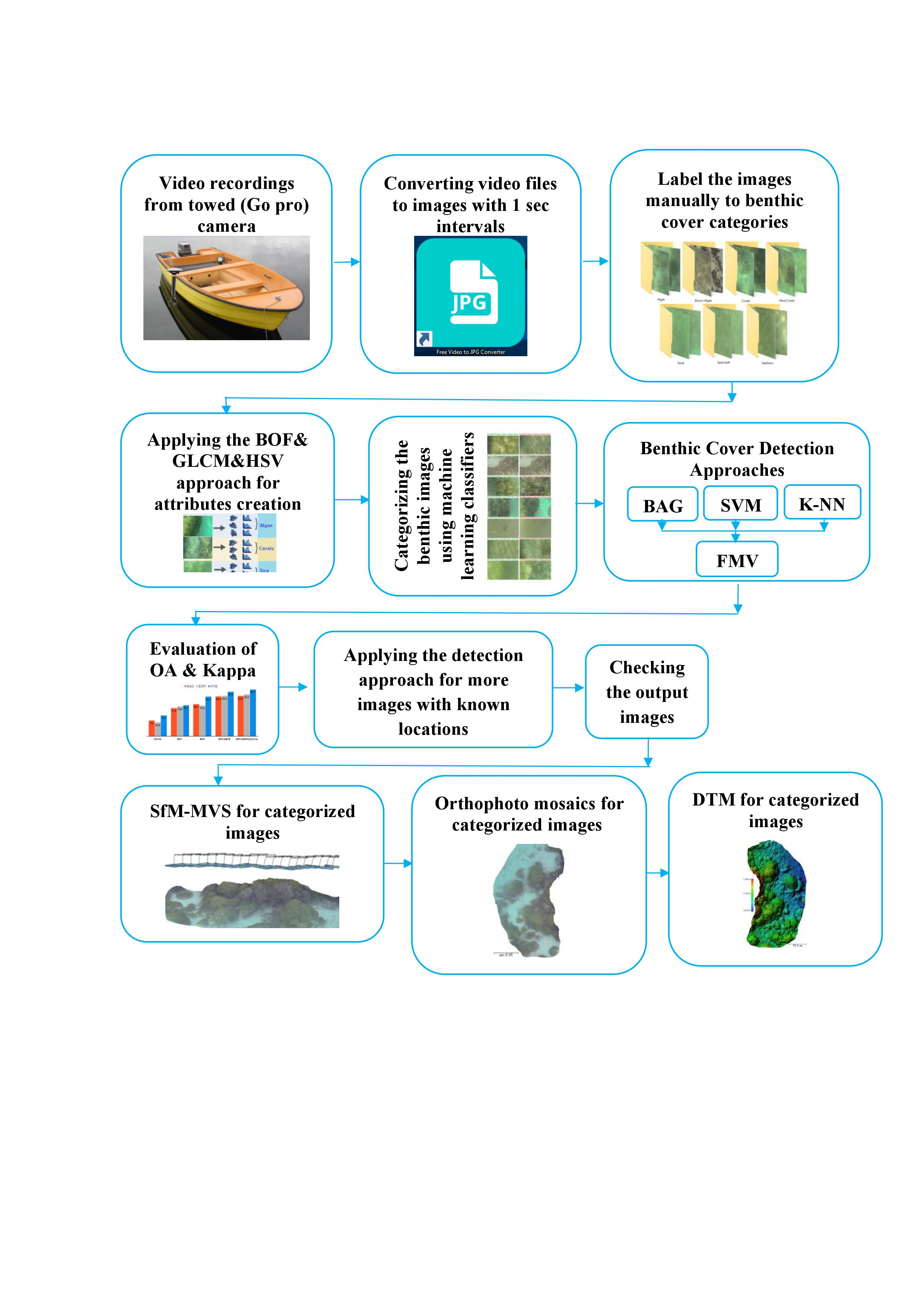
The study site is located in the Shiraho subtropical region, which is included partly in the southeastern part of Ishigaki Island, Japan (see Figure 1). This is an area rich in marine biodiversity, with shallow, low-turbidity water [47] and a maximum depth of 3.5 m. The Shiraho area has various reefscapes, including complex patches of branching (Acropora) and massive corals (Porites). Moreover, it has a large colony of a Blue Ridge coral (Heliopora coerulea). There are also a wide range of brown algae and blue algae, a variety of geomorphic features (soft sand, cobble, and boulders), and seagrass.
2.2. Benthic Cover Field Data
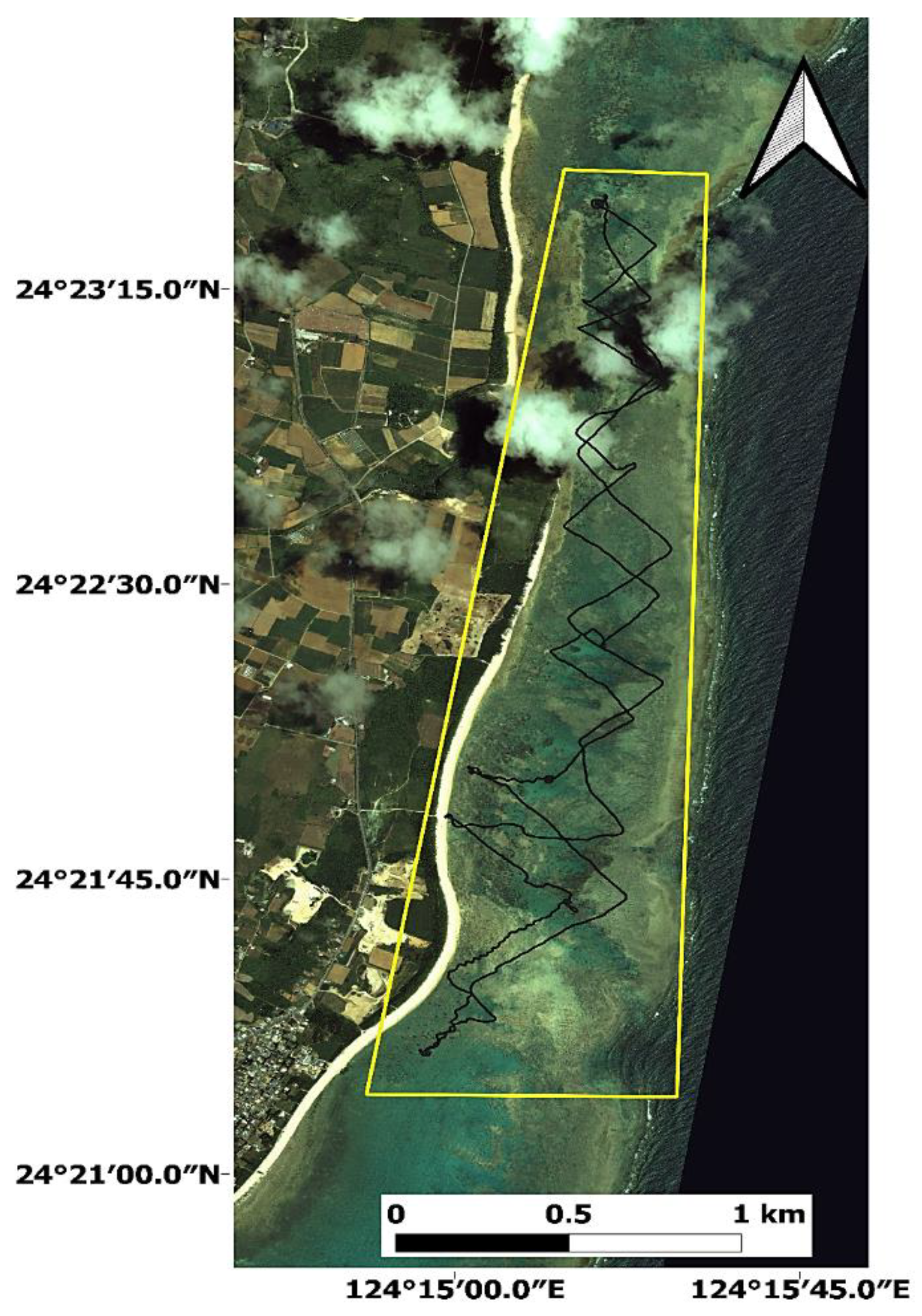
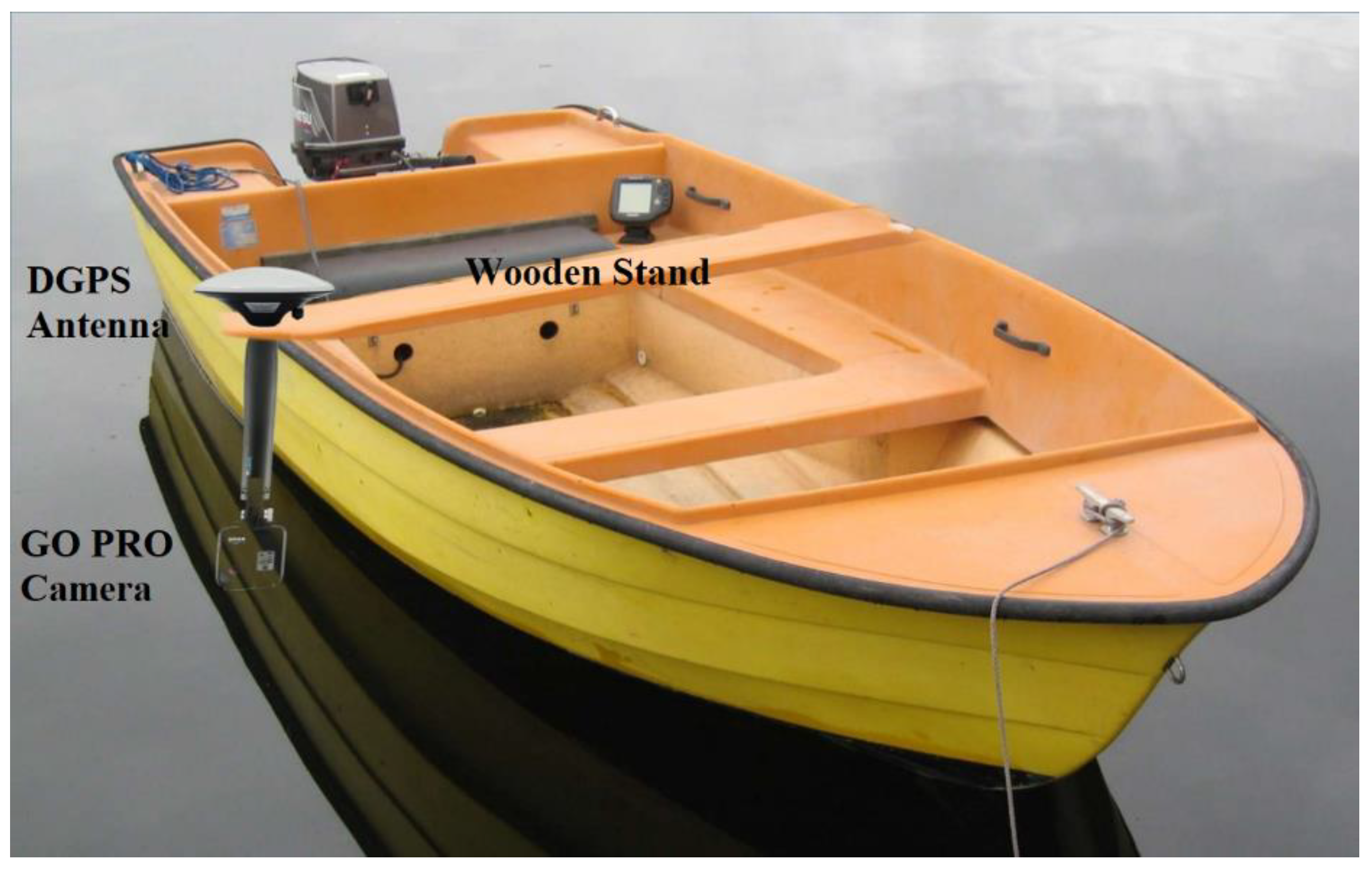
Benthic cover field data collection began on 21 August 2016 (see Figure 1). Underwater videos were obtained using a low-cost compact high-resolution camcorder (GoPro HERO3 Black Edition, 1440 video resolution, 30 frames per second with a wide field of view). The utilized GoPro HERO3 camera has stable interior orientation parameters (IOPs) [48]. The camcorder was attached beneath the surveying motorboat side just under the surface of the water to observe the shallow seabed. A series of four hours of video recordings from the survey trip were acquired. These recordings were geolocated using a differential global positioning system (DGPS) system mounted vertically by a wooden stand above the camera. Figure 2 is an illustrative picture to describe the DGPS and the camera positions on the motorboat. A free video to image converter software package was used to extract images from the video files with a one-second image interval and a minimum 60% overlap to be synchronized with the DGPS surveys. The DGPS kinematic observations were post processed using the online Natural Resources Canada Precise Point Positioning (PPP) service (https://webapp.geod.nrcan.gc.ca/geod/tools-outils/ppp.php), thereby achieving centimeter-level accuracy. To properly locate the camera center points, 55 cm was subtracted in the Z direction, which was the distance between the receiver antenna and the camera position. The resulting positions were used as the camera positions in the 3D model production input process. From the extracted images, 3000 images with known locations (using the DGPS system) were labeled manually for seven classes (see Figure 3).
2.3. Methodology
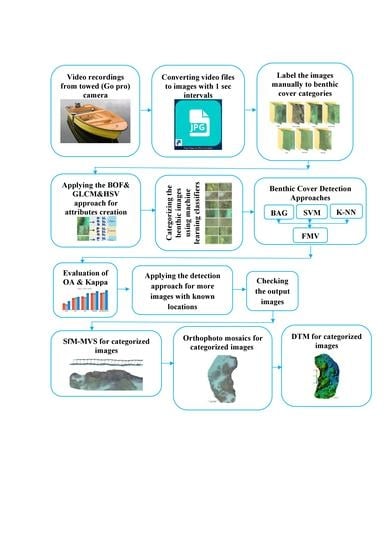
The proposed framework for benthic cover classification and 3D mapping over the Shiraho area was established as follows:
- All four hours of the video recordings were converted to geolocated images using a free video to JPG converter program with one-second intervals synchronized with the DGPS recorded locations.
- A total of 3000 converted images were labeled individually by a human expert according to seven benthic cover categories: corals (Acropora and Porites), blue corals (H. coerulea), brown algae, blue algae, soft sand, hard sediments (pebbles, cobbles, and boulders), and seagrass.
- These labeled geolocated images were used as inputs for the BOF, Hue Saturation Value (HSV), and Gray Level Co-occurrence Matrix (GLCM) approaches to create the attributes for the semiautomatic classification.
- The extracted attributes produced from the BOF, HSV, and GLCM approaches were used as the inputs for training three machine learning soft classifiers (BAG, SVM, and k-NN), and the image labels were used as the outputs.
- The three classifiers were combined with the FMV algorithm to classify the benthic cover categories.
- The entire classifier evaluation process was conducted using 2250 independent randomly sampled images (75%) for training and 750 images (25%) for testing.
- After the FMV algorithm was trained and validated, it was used to categorize more images, and the resulting images were checked individually.
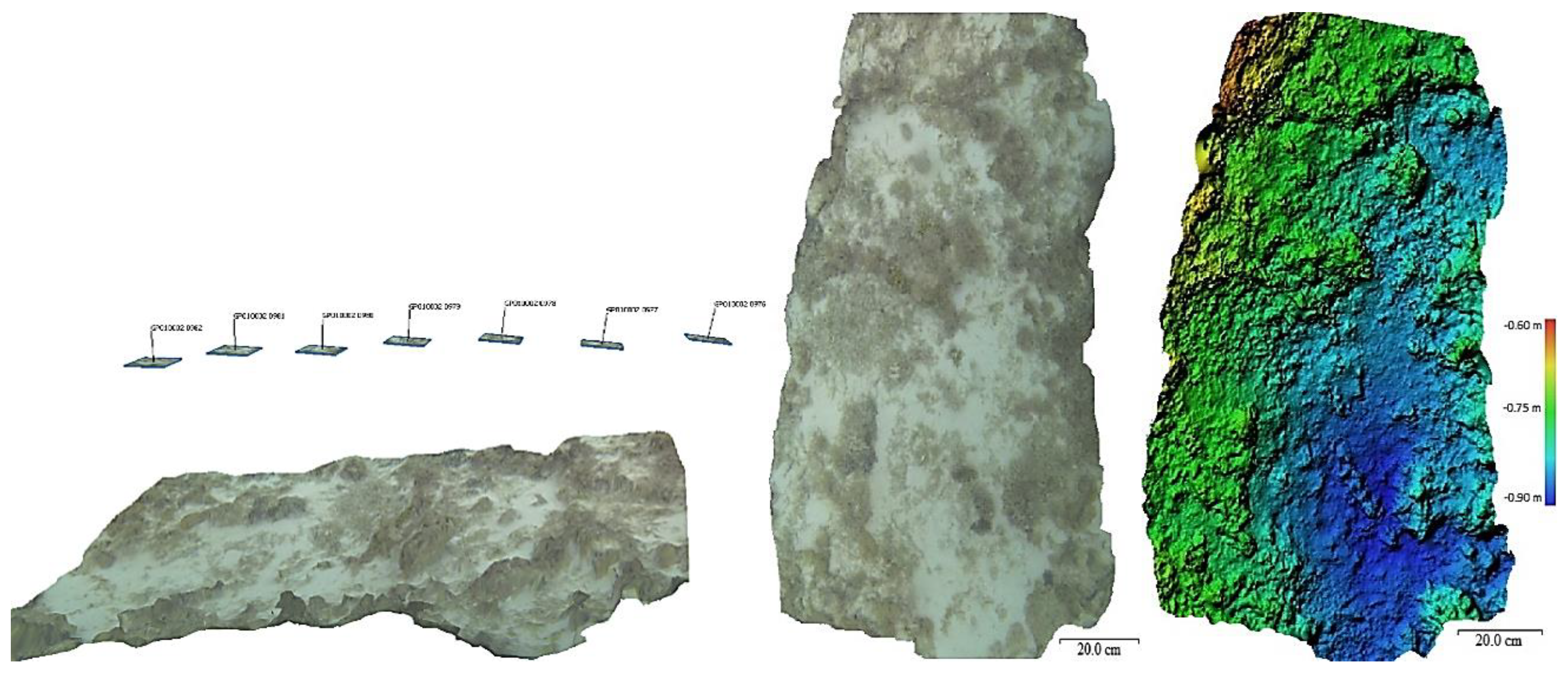
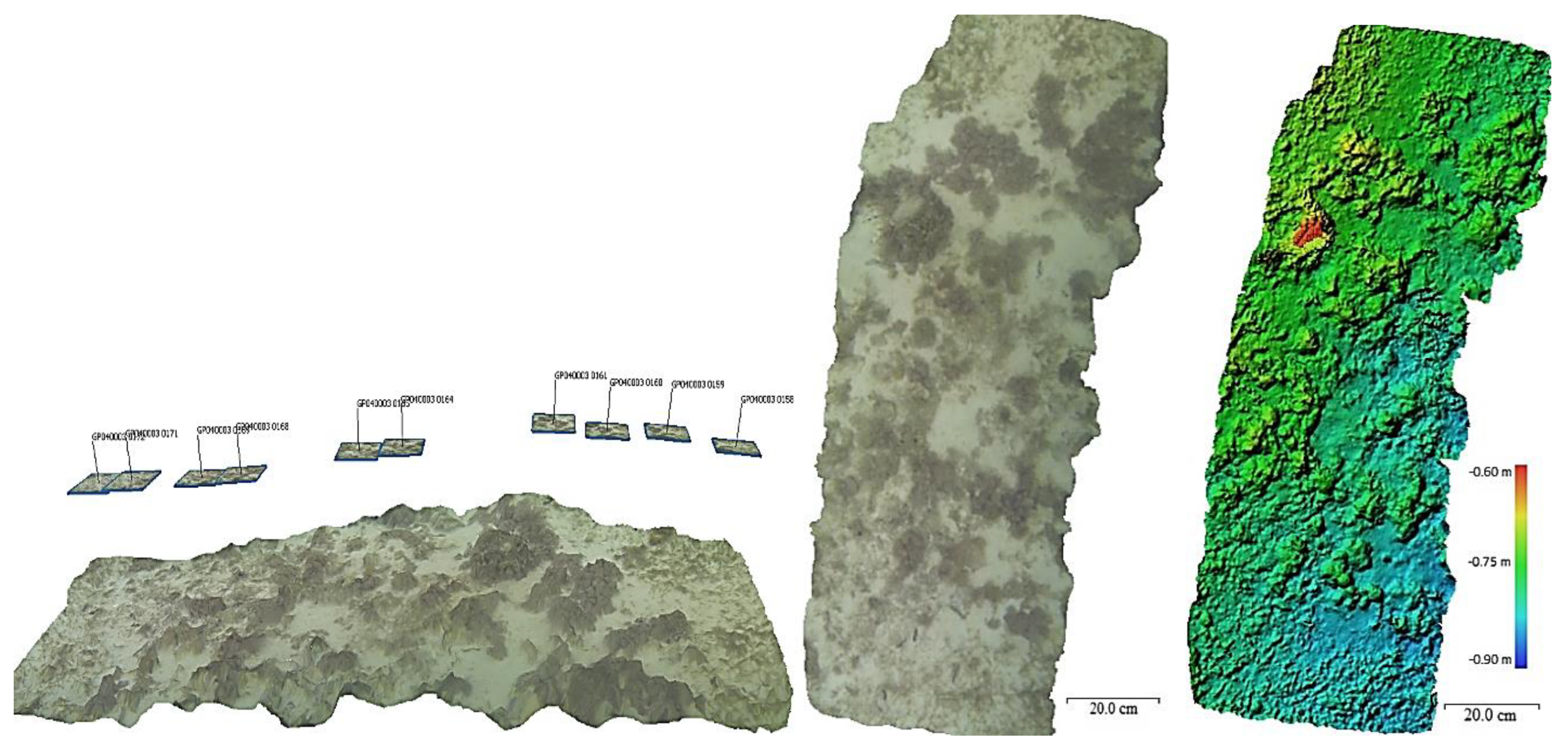
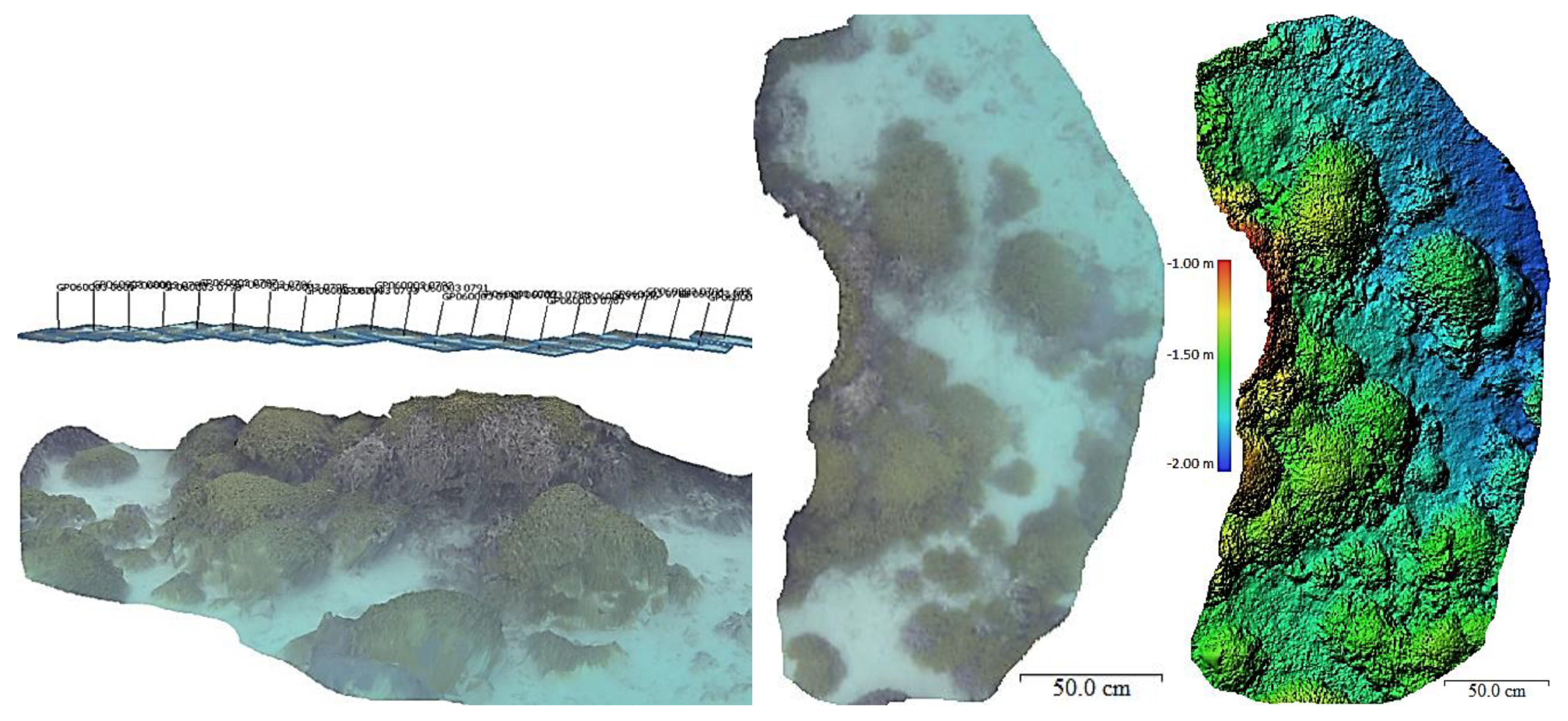
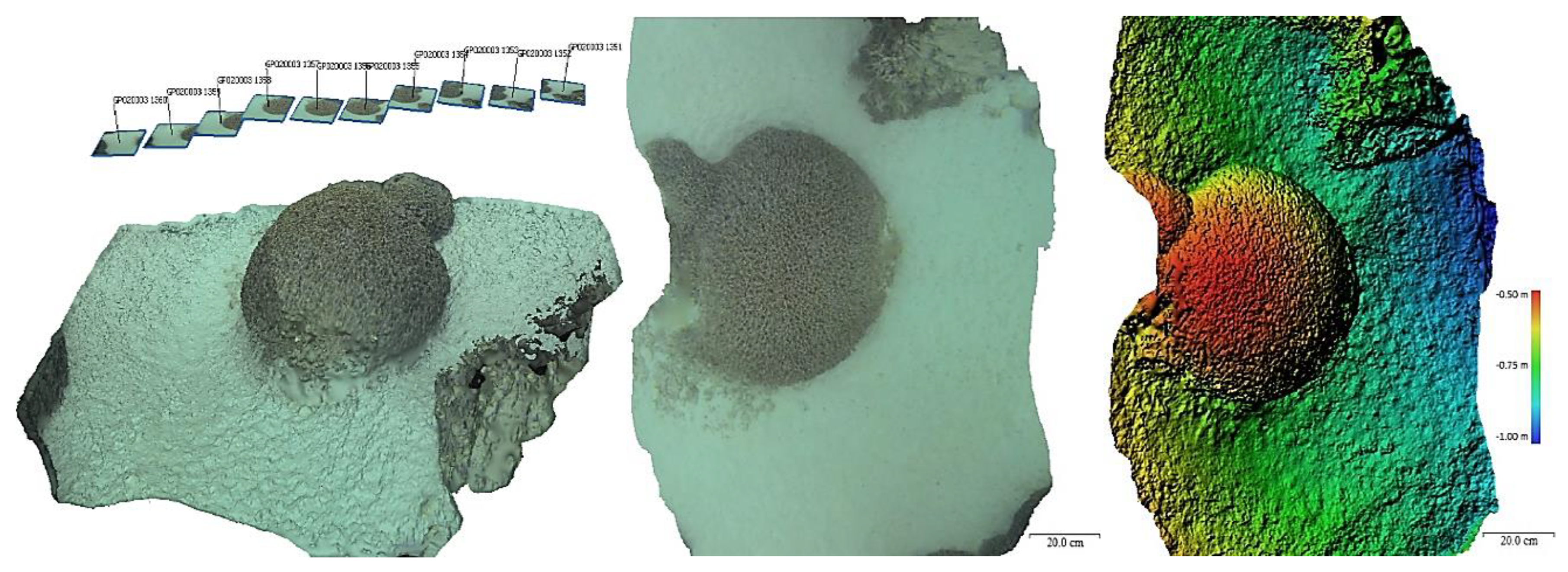
- SfM-MVS techniques were performed to produce 3D mosaics and digital terrain models DTMs for each habitat class using the correctly categorized geolocated JPG images.
The entire benthic cover classification process was applied in the MATLAB environment, with the following described parameters for each method.
For extracting benthic habitat categorization attributes, 26 texture parameters, 256 HSV values, and 250 BOF attributes were extracted from each image using the MATLAB environment (see Table 1).
We tested the principal component analysis approach for removing redundancies from the input attributes, but the OA decreased significantly to 75%.
Subsequently, to classify benthic cover, BAG [49,50], SVM [51,52], and k-NN [53,54] soft classifiers were used with the following parameters. The BAG approach assembled 30 classification trees with 24 splits for each tree; the SVM model used a third-order polynomial kernel function; and the k-NN approach had five neighbors for the k-value, used the city block technique for distance calculation, and used the squared inverse distance weight as the distance weighting function method. For each algorithm, these parameters produced the highest OA and Kappa values. Finally, the resulting probabilities from each soft classifier were ensembled using the FMV [55,56] model.
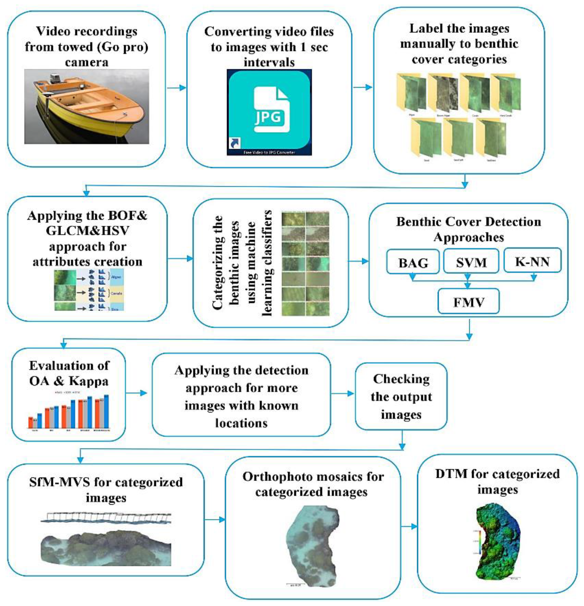
Agisoft PhotoScan Professional software was used to produce the 3D categorized DTMs and orthophoto mosaics based on the SfM-MVS approaches. Four steps were used, and the parameters of each step were chosen according to the recommended settings by the software developers and performed trials. The first step, known as photo alignment, uses the post processed camera positions in the input process. This step includes computing the initially estimated IOPs using a scale invariant feature transform matching algorithm. Then, a local reference coordinate system is established to create the initial datum for determining the images’ exterior orientation parameters and the 3D coordinates of the matched points [48]. Second, a bundle adjustment procedure is performed to adjust the exterior orientation parameters, and object coordinates are created in the first step [57]. Third, a dense point cloud with ultrahigh quality is generated based on the MVS technique. Then, a mesh is created using the dense point cloud with an arbitrary surface type, thereby enabling interpolation for the final model generation. Fourth, a texture atlas with a generic mapping mode for the model is built and used to generate the orthophoto mosaic. Finally, all the categorized DTMs and orthophoto mosaics produced are exported with a pixel resolution of 5 cm. The proposed methodology for this research was applied in several key procedures, as shown in Figure 4.
3. Results
Figure 5 show examples of correct and misclassified benthic cover categories resulting from the proposed FMV algorithm. Additionally, the numbers of the correct species categorized from the k-NN, BAG, and SVM classifiers using different attributes are illustrated in Figure 6. Table 2 summarizes the corresponding OA and Kappa values for k-NN, BAG, SVM, and FMV ensemble classifiers, and Table 3 presents the confusion matrix for the classification of benthic habitats using the FMV ensemble. Figure 7, Figure 8, Figure 9, Figure 10 and Figure 11 show a sample of the correctly categorized 3D views, orthophoto mosaics, and DTMs for each.
4. Discussion
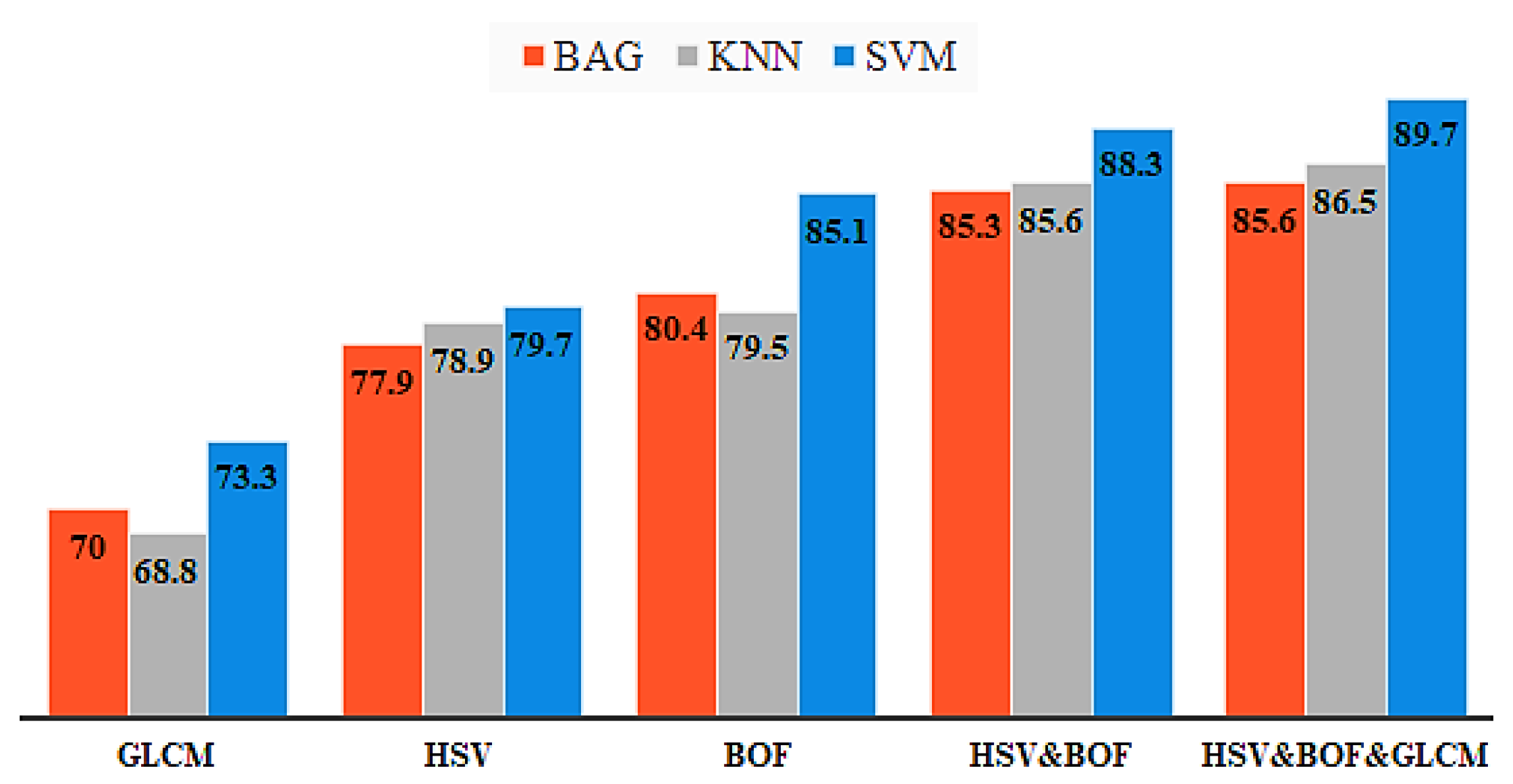
In our study, we investigated the discrimination attributes of various benthic cover features. A comparison was made between 256 HSV visual values, 26 GLCM texture values, and 250 BOF values for benthic cover classification. BOF attributes produced the highest species discrimination accuracy, followed by HSV predictors and the GLCM texture values. Additionally, compared to using any single predictor, assembling three predictor groups improved the accuracy of species classification.
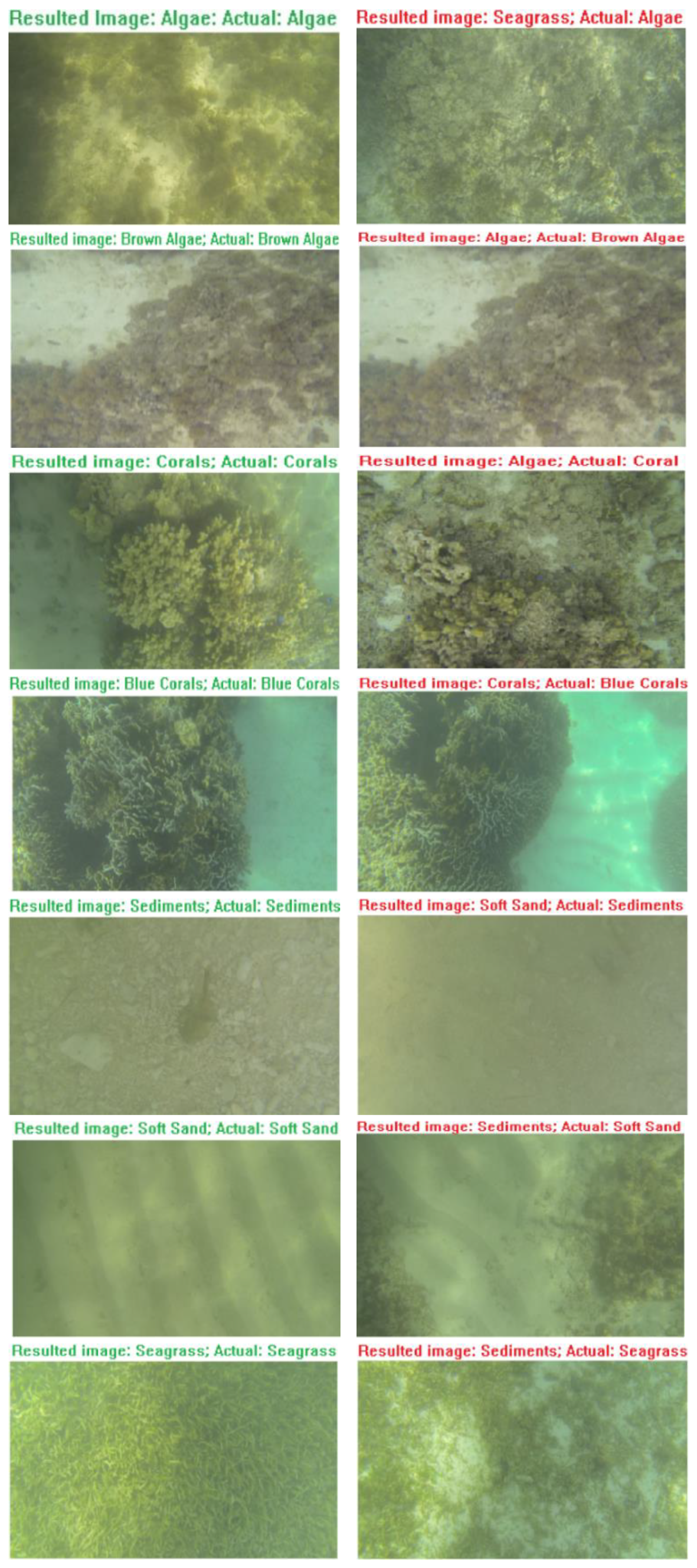
The extracted benthic cover attributes were used as the input for three SVM, BAG, and k-NN supervised classifiers. These supervised classifiers were selected following numerous trials based on the highest OA and Kappa values. Numerous classifiers, such as boosting trees, maximum likelihood, and neural network, were tested for benthic classification but yielded lower OA values. SVM produced significantly better results for all benthic cover species’ classification compared to both the k-NN and BAG classifiers. The most challenging part of this process was discriminating between soft sand and sediments or corals and blue corals. The mixture of soft sand and sediments in most benthic cover created confusion for all classifiers. In addition, in most of the benthic cover images, the blue corals and corals were difficult to distinguish visually. In addition, the noise of the images, coupled with the poor lighting and water turbidity, impacted the accuracy of discrimination for all classifiers. Nevertheless, the algae, brown algae, and seagrass species were classified with high accuracy (see Table 3).
Chagoonian et al. [58] proved that soft classifiers are more accurate in coral reef mapping compared to traditional hard classifiers. As a result, together, these classifiers can produce more informative maps, especially in very heterogeneous coral reef environments. Moreover, it has been proven in recent studies (e.g., [59,60,61]) that ensemble approaches outperform single classifiers in benthic cover mapping. The proposed FMV ensemble in our study readily combines the probabilities resulting from BAG, SVM, and k-NN soft classifiers that were trained independently. These soft classifiers resulted in diverse per-class accuracy, caused mainly by the differences in their concepts. The FMV ensemble increased the OA and Kappa values for benthic cover classification from the three base classifiers from approximately 4% and 0.05 to 93.5% and 0.92, respectively. These findings demonstrate that the FMV ensemble produces higher classification accuracy compared to the BAG, SVM, and k-NN classifiers used in benthic cover classification.
In this study, we performed benthic habitat classification semiautomatically using visual, texture, and color attributes and then produced 3D categorized thematic maps using SfM-MVS algorithms. Such 3D maps can be used to measure the physical aspects of corals, such as volume, surface roughness, and the proportion of living and/or dead corals [28,29,30,31,32,33,34,35]. The fine scales targeted in this study significantly improve the spatial resolution of diagnoses and predictions for coral reefs. SfM-MVS techniques were performed successfully to produce categorized 3D models for five benthic habitats; only soft sand and sediments were excluded. However, these techniques failed, in a few cases, to align the overlapped images. These cases included poor quality images with low illumination over turbid areas produced from the towed camera. Furthermore, the most complicated areas were located at seagrass meadows; since seagrass frequently moves via waves and currents, 3D mapping of the seagrass canopy was difficult.
In summary, the proposed benthic cover classification and 3D mapping system has many advantages and involves simpler logistics than current methods. The required geolocated images can be obtained using a low-cost towed camera that can be mounted beneath a small motorboat with a DGPS system. These field surveys do not harm the surrounding environment and can be repeated annually to monitor the health of benthic habitats using the same FMV ensemble. The resulting high-resolution 3D maps can be used to monitor either the bleaching of coral reefs or their spatial and temporal changes. Finally, compared with deep learning algorithms, the present approach requires simple programs with relatively short processing times, labor requirements, and a small number of field images needed to train classifiers. Nevertheless, there are some drawbacks requiring improvement (e.g., the limitation in complex mixed areas or high-turbidity areas and limited shallow areas, which can be processed). Still, these results should encourage further studies on the proposed approach, such as using ROV systems to produce higher-quality images for monitoring deep seafloor areas [30]. Moreover, studying the same proposed approaches with the new Fluid lensing optical multispectral instrument (FluidCam) and Multispectral Imaging Detection and Active Reflectance instrument (MiDAR) developed by NASA [62]. FluidCam can produce 3D multispectral images corrected from refraction for shallow marine environments. Also, MiDAR is an active multispectral sensor that illuminates targets with high-intensity narrowband radiation to produce multispectral images across the ultraviolet, visible, and near-infrared bands. The additional multispectral bands can be used to increase the classification accuracy over the heterogeneous areas. Finally, testing the performance of image enhancement techniques for increasing the towed camera images quality and reducing the turbidity and caustics effects.
5. Conclusions
The SfM-MVS approaches and machine learning algorithms are effective tools for monitoring coastal areas, particularly vulnerable shallow habitats where species are threatened by climate change and human activity [31]. Recently, more attempts have been performed to apply both techniques for generating high-resolution 3D information. In this study, we applied SfM-MVS and machine learning algorithms to produce high-resolution categorized 3D habitat maps. The framework presented herein was tested for classifying seven species in the Shiraho heterogeneous coastal area of Japan. The framework was constructed as follows: the semiautomatic classification of benthic habitats was based on the BOF, HSV, and GLCM attributes’ extraction techniques. Several attributes were extracted and assessed from labeled examples using video images from a towed video camera; these examples were geolocated by the DGPS system. Three soft classifiers, k-NN, SVM, and BAG outputs, were assembled by the FMV algorithm. Our results show that the semiautomatic classification of the seven habitats was produced with an OA of 92.7% using the FMV algorithm. Second, fine-scale 3D products like DTMs and ortho mosaics were generated for the correctly categorized georeferenced images using the SfM-MVS techniques. These products are vital for studying topography, rugosity, and the other structural characteristics of benthic communities. The simplicity of this framework facilitates its repeatability and opens the possibility of generating usable products for a broad range of ecological applications.
Author Contributions
Conceptualization, H.M., K.N. and T.N.; data curation, H.M. and T.N.; formal analysis, H.M. and K.N.; funding acquisition, K.N.; investigation, T.N.; methodology, H.M.; project administration, K.N.; resources, T.N.; software, H.M.; supervision, K.N.; validation, H.M. and T.N.; writing—original draft, H.M.; writing—review & editing, K.N. and T.N. All authors have read and agreed to the published version of the manuscript.
Funding
This research was financially supported partly by the Egyptian Ministry of Higher Education, Nadaoka Laboratory in Tokyo Institute of Technology and JSPS Grant-in-Aids for Scientific Research (No. 15H02268), and Science and Technology Research Partnership for Sustainable Development (SATREPS) program, Japan Science and Technology Agency (JST)/Japan International Cooperation Agency (JICA).
Conflicts of Interest
The authors declare no conflict of interest.
References
- Hossain, M.S.; Bujang, J.S.; Zakaria, M.H.; Hashim, M. The application of remote sensing to seagrass ecosystems: An overview and future research prospects. Int. J. Remote Sens. 2015, 36, 61–114. [Google Scholar] [CrossRef]
- Vassallo, P.; Bianchi, C.N.; Paoli, C.; Holon, F.; Navone, A.; Bavestrello, G.; Cattaneo Vietti, R.; Morri, C. A predictive approach to benthic marine habitat mapping: Efficacy and management implications. Mar. Pollut. Bull. 2018, 131, 218–232. [Google Scholar] [CrossRef] [PubMed]
- Gauci, A.; Deidun, A.; Abela, J.; Zarb Adami, K. Machine Learning for benthic sand and maerl classification and coverage estimation in coastal areas around the Maltese Islands. J. Appl. Res. Technol. 2016, 14, 338–344. [Google Scholar] [CrossRef] [Green Version]
- Anderson, T.J.; Cochrane, G.R.; Roberts, D.A.; Chezar, H.; Hatcher, G. A rapid method to characterize seabed habitats and associated macro-organisms. Mapp. Seafloor Habitat Charact. Geol. Assoc. Can. Spec. Pap. 2007, 47, 71–79. [Google Scholar]
- Smith, J.; O’Brien, P.E.; Stark, J.S.; Johnstone, G.J.; Riddle, M.J. Integrating multibeam sonar and underwater video data to map benthic habitats in an East Antarctic nearshore environment. Estuar. Coast. Shelf Sci. 2015, 164, 520–536. [Google Scholar] [CrossRef]
- Mallet, D.; Pelletier, D. Underwater video techniques for observing coastal marine biodiversity: A review of sixty years of publications (1952–2012). Fish. Res. 2014, 154, 44–62. [Google Scholar] [CrossRef]
- Hamylton, S.M. Mapping coral reef environments: A review of historical methods, recent advances and future opportunities. Prog. Phys. Geogr. 2017, 41, 803–833. [Google Scholar] [CrossRef]
- Roelfsema, C.; Kovacs, E.; Roos, P.; Terzano, D.; Lyons, M.; Phinn, S. Use of a semi-automated object based analysis to map benthic composition, Heron Reef, Southern Great Barrier Reef. Remote Sens. Lett. 2018, 9, 324–333. [Google Scholar] [CrossRef]
- Roelfsema, C.; Lyons, M.; Dunbabin, M.; Kovacs, E.M.; Phinn, S. Integrating field survey data with satellite image data to improve shallow water seagrass maps: The role of AUV and snorkeller surveys? Remote Sens. Lett. 2015, 6, 135–144. [Google Scholar] [CrossRef]
- Zapata-Ramírez, P.A.; Blanchon, P.; Olioso, A.; Hernandez-Nuñez, H.; Sobrino, J.A. Accuracy of IKONOS for mapping benthic coral-reef habitats: A case study from the Puerto Morelos Reef National Park, Mexico. Int. J. Remote Sens. 2012, 34, 3671–3687. [Google Scholar]
- Seiler, J.; Friedman, A.; Steinberg, D.; Barrett, N.; Williams, A.; Holbrook, N.J. Image-based continental shelf habitat mapping using novel automated data extraction techniques. Cont. Shelf Res. 2012, 45, 87–97. [Google Scholar] [CrossRef]
- Bewley, M.; Friedman, A.; Ferrari, R.; Hill, N.; Hovey, R.; Barrett, N.; Pizarro, O.; Figueira, W.; Meyer, L.; Babcock, R.; et al. Australian sea-floor survey data, with images and expert annotations. Sci. Data 2015, 2, 150057. [Google Scholar] [CrossRef] [PubMed]
- Pante, E.; Dustan, P. Getting to the Point: Accuracy of Point Count in Monitoring Ecosystem Change. J. Mar. Biol. 2012, 2012, 802875. [Google Scholar] [CrossRef] [Green Version]
- Rigby, P.; Pizarro, O.; Williams, S.B. Toward Adaptive Benthic Habitat Mapping Using Gaussian Process Classification. J. Field Robot. 2010, 27, 741–758. [Google Scholar] [CrossRef]
- Singh, H.; Howland, J.; Pizarro, O. Advances in large-area photomosaicking underwater. IEEE J. Ocean. Eng. 2004, 29, 872–886. [Google Scholar] [CrossRef]
- Agrafiotis, P.; Skarlatos, D.; Forbes, T.; Poullis, C.; Skamantzari, M.; Georgopoulos, A. Underwater photogrammetry in very shallow waters: Main challenges and caustics effect removal. In Proceedings of the International Archives of the Photogrammetry, Remote Sensing and Spatial Information Sciences—ISPRS Archives, Riva del Garda, Italy, 4–7 June 2018; pp. 15–22. [Google Scholar]
- Elnashef, B.; Filin, S. Direct linear and refraction-invariant pose estimation and calibration model for underwater imaging. ISPRS J. Photogramm. Remote Sens. 2019, 154, 259–271. [Google Scholar] [CrossRef]
- Guinan, J.; Brown, C.; Dolan, M.F.J.; Grehan, A.J. Ecological Informatics Ecological niche modelling of the distribution of cold-water coral habitat using underwater remote sensing data. Ecol. Inf. 2009, 4, 83–92. [Google Scholar] [CrossRef]
- Baumstark, R.; Duffey, R.; Pu, R. Mapping seagrass and colonized hard bottom in Springs Coast, Florida using WorldView-2 satellite imagery. Estuar. Coast. Shelf Sci. 2016, 181, 83–92. [Google Scholar] [CrossRef]
- Baumstark, R.; Dixon, B.; Carlson, P.; Palandro, D.; Kolasa, K. Alternative spatially enhanced integrative techniques for mapping seagrass in Florida’s marine ecosystem. Int. J. Remote Sens. 2013, 34, 1248–1264. [Google Scholar] [CrossRef]
- Javernick, L.; Brasington, J.; Caruso, B. Modeling the topography of shallow braided rivers using Structure-from-Motion photogrammetry. Geomorphology 2014, 213, 166–182. [Google Scholar] [CrossRef]
- Burns, J.H.R.; Delparte, D.; Gates, R.D.; Takabayashi, M. Integrating structure-from-motion photogrammetry with geospatial software as a novel technique for quantifying 3D ecological characteristics of coral reefs. PeerJ 2015, 3, e1077. [Google Scholar] [CrossRef] [PubMed]
- Westoby, M.J.; Brasington, J.; Glasser, N.F.; Hambrey, M.J.; Reynolds, J.M. “Structure-from-Motion” photogrammetry: A low-cost, effective tool for geoscience applications. Geomorphology 2012, 179, 300–314. [Google Scholar] [CrossRef] [Green Version]
- Fonstad, M.A.; Dietrich, J.T.; Courville, B.C.; Jensen, J.L.; Carbonneau, P.E. Topographic structure from motion: A new development in photogrammetric measurement. Earth Surf. Process. Landf. 2013, 38, 421–430. [Google Scholar] [CrossRef] [Green Version]
- Piazza, P.; Cummings, V.; Guzzi, A.; Hawes, I.; Lohrer, A.; Marini, S.; Marriott, P.; Menna, F.; Nocerino, E.; Peirano, A.; et al. Underwater photogrammetry in Antarctica: Long-term observations in benthic ecosystems and legacy data rescue. Polar Biol. 2019, 42, 1061–1079. [Google Scholar] [CrossRef] [Green Version]
- Xiao, X.; Guo, B.; Li, D.; Li, L.; Yang, N.; Liu, J.; Zhang, P.; Peng, Z. Multi-view stereo matching based on self-adaptive patch and image grouping for multiple unmanned aerial vehicle imagery. Remote Sens. 2016, 8, 89. [Google Scholar] [CrossRef] [Green Version]
- Bryson, M.; Ferrari, R.; Figueira, W.; Pizarro, O.; Madin, J.; Williams, S.; Byrne, M. Characterization of measurement errors using structure—Motion and photogrammetry to measure marine habitat structural complexity. Ecol. Evol. 2017, 5669–5681. [Google Scholar] [CrossRef]
- Leon, J.X.; Roelfsema, C.M.; Saunders, M.I.; Phinn, S.R. Measuring coral reef terrain roughness using “Structure-from-Motion” close-range photogrammetry. Geomorphology 2015, 242, 21–28. [Google Scholar] [CrossRef]
- Palma, M.; Casado, M.R.; Pantaleo, U.; Pavoni, G.; Pica, D.; Cerrano, C. SfM-based method to assess gorgonian forests (Paramuricea clavata (Cnidaria, Octocorallia)). Remote Sens. 2018, 10, 1154. [Google Scholar] [CrossRef] [Green Version]
- Pizarro, O.; Eustice, R.M.; Singh, H. Large area 3-D reconstructions from underwater optical surveys. IEEE J. Ocean. Eng. 2009, 34, 150–169. [Google Scholar] [CrossRef] [Green Version]
- Agrafiotis, P.; Skarlatos, D.; Georgopoulos, A.; Karantzalos, K. DepthLearn: Learning to Correct the Refraction on Point Clouds Derived from Aerial Imagery for Accurate Dense Shallow Water Bathymetry Based on SVMs-Fusion with LiDAR Point Clouds. Remote Sens. 2019, 11, 2225. [Google Scholar] [CrossRef] [Green Version]
- Casella, E.; Collin, A.; Harris, D.; Ferse, S.; Bejarano, S.; Parravicini, V.; Hench, J.L.; Rovere, A. Mapping coral reefs using consumer-grade drones and structure from motion photogrammetry techniques. Coral Reefs 2017, 36, 269–275. [Google Scholar] [CrossRef]
- Dietrich, J.T. Bathymetric Structure-from-Motion: Extracting shallow stream bathymetry from multi-view stereo photogrammetry. Earth Surf. Process. Landf. 2017, 42, 355–364. [Google Scholar] [CrossRef]
- Figueira, W.; Ferrari, R.; Weatherby, E.; Porter, A.; Hawes, S.; Byrne, M. Accuracy and precision of habitat structural complexity metrics derived from underwater photogrammetry. Remote Sens. 2015, 7, 16883–16900. [Google Scholar] [CrossRef] [Green Version]
- Storlazzi, C.D.; Dartnell, P.; Hatcher, G.A.; Gibbs, A.E. End of the chain? Rugosity and fine-scale bathymetry from existing underwater digital imagery using structure-from-motion (SfM) technology. Coral Reefs 2016, 35, 889–894. [Google Scholar] [CrossRef]
- Raoult, V.; Reid-Anderson, S.; Ferri, A.; Williamson, J. How Reliable Is Structure from Motion (SfM) over Time and between Observers? A Case Study Using Coral Reef Bommies. Remote Sens. 2017, 9, 740. [Google Scholar] [CrossRef] [Green Version]
- Ahsan, N.; Williams, S.B.; Jakuba, M.; Pizarro, O.; Radford, B. Predictive habitat models from AUV-based multibeam and optical imagery. In Proceedings of the OCEANS 2010 MTS/IEEE SEATTLE, Seattle, WA, USA, 20–23 September 2010; pp. 1–10. [Google Scholar]
- Price, D.M.; Robert, K.; Callaway, A.; Lo lacono, C.; Hall, R.A.; Huvenne, V.A.I. Using 3D photogrammetry from ROV video to quantify cold-water coral reef structural complexity and investigate its influence on biodiversity and community assemblage. Coral Reefs 2019, 38, 1007–1021. [Google Scholar] [CrossRef] [Green Version]
- Williams, S.B.; Pizarro, O.; Mahon, I.; Johnson-Roberson, M. Simultaneous Localisation and Mapping and Dense Stereoscopic Seafloor Reconstruction Using an AUV. In Proceedings of the Experimental Robotics; Khatib, O., Kumar, V., Pappas, G.J., Eds.; Springer: Berlin/Heidelberg, Germany, 2009; pp. 407–416. [Google Scholar]
- Pavoni, G.; Corsini, M.; Callieri, M.; Palma, M.; Scopigno, R. SEMANTIC SEGMENTATION of BENTHIC COMMUNITIES from ORTHO-MOSAIC MAPS. In Proceedings of the ISPRS Annals of the Photogrammetry, Remote Sensing and Spatial Information Sciences; ISPRS: Limassol, Cyprus, 2019; Volume XLII-2/W10, pp. 151–158. [Google Scholar]
- Liu, Z.-G.; Zhang, X.-Y.; Yang, Y.; Wu, C.-C. A Flame Detection Algorithm Based on Bag-of—Features In The YUV Color Space. In Proceedings of the International Conference on Intelligent Computing and Internet of Things (IC1T), Chongqing, China, 21–23 September 2015; pp. 64–67. [Google Scholar]
- Nazir, S.; Yousaf, M.H.; Velastin, S.A. Evaluating a bag-of-visual features approach using spatio-temporal features for action recognition. Comput. Electr. Eng. 2018, 72, 660–669. [Google Scholar] [CrossRef]
- Shi, R.B.; Qiu, J.; Maida, V. Towards algorithm-enabled home wound monitoring with smartphone photography: A hue-saturation-value colour space thresholding technique for wound content tracking. Int. Wound J. 2018, 16, 211–218. [Google Scholar] [CrossRef] [Green Version]
- Mazumder, J.; Nahar, L.N. Moin Uddin Atique Finger Gesture Detection and Application Using Hue Saturation Value. Int. J. Image Graph. Signal Process. 2018, 8, 31–38. [Google Scholar] [CrossRef]
- Zheng, G.; Li, X.; Member, S.; Zhou, L.; Yang, J.; Ren, L.; Chen, P.; Zhang, H.; Lou, X. Development of a Gray-Level Co-Occurrence Matrix-Based Texture Orientation Estimation Method and Its Application in Sea Surface Wind Direction Retrieval From SAR Imagery. IEEE Trans. Geosci. Remote Sens. 2018, 56, 1–17. [Google Scholar] [CrossRef]
- Moya, L.; Zakeri, H.; Yamazaki, F.; Liu, W.; Mas, E.; Koshimura, S. 3D gray level co-occurrence matrix and its application to identifying collapsed buildings. ISPRS J. Photogramm. Remote Sens. 2019, 149, 14–28. [Google Scholar] [CrossRef]
- Paringit, E.C.; Nadaoka, K. Simultaneous estimation of benthic fractional cover and shallow water bathymetry in coral reef areas from high-resolution satellite images. Int. J. Remote 2012, 33, 3026–3047. [Google Scholar] [CrossRef]
- He, F.; Habib, A. Target-based and feature-based calibration of low-cost digital cameras with large field-of-view. In Proceedings of the IGTF 2015—ASPRS Annual Conference, Tampa, FL, USA, 4–8 May 2015; pp. 205–212. [Google Scholar]
- Breiman, L. Bagging Predictors. Mach. Learn. 1996, 24, 123–140. [Google Scholar] [CrossRef] [Green Version]
- Tien, D.; Ho, B.T.; Pradhan, B.; Pham, B. GIS-based modeling of rainfall-induced landslides using data mining-based functional trees classifier with AdaBoost, Bagging, and MultiBoost ensemble frameworks. Environ. Earth Sci. 2016, 75, 1–22. [Google Scholar] [CrossRef]
- CORTES, C.; VAPNIK, V. Support-Vector Networks. Mach. Learn. 1995, 20, 273–297. [Google Scholar] [CrossRef]
- Ishida, H.; Oishi, Y.; Morita, K.; Moriwaki, K.; Nakajima, T.Y. Development of a support vector machine based cloud detection method for MODIS with the adjustability to various conditions. Remote Sens. Environ. 2018, 205, 390–407. [Google Scholar] [CrossRef]
- Noi, P.T.; Kappas, M. Comparison of Random Forest, k-Nearest Neighbor, and Support Vector Machine Classifiers for Land Cover Classification Using Sentinel-2 Imagery. Sensors 2018, 18, 18. [Google Scholar]
- Shihavuddin, A.S.M.; Gracias, N.; Garcia, R.; Gleason, A.C.R.; Gintert, B. Image-based coral reef classification and thematic mapping. Remote Sens. 2013, 5, 1809–1841. [Google Scholar] [CrossRef] [Green Version]
- Salah, M. Fuzzy Majority Voting based fusion of Markovian probability for improved Land Cover Change Prediction. Int. J. Geoinform. 2016, 12, 27–40. [Google Scholar]
- Valdivia, A.; Luzíón, M.V.; Herrera, F. Neutrality in the sentiment analysis problem based on fuzzy majority. In Proceedings of the 2017 IEEE International Conference on Fuzzy Systems (FUZZ-IEEE), Naples, Italy, 9–12 July 2017; pp. 1–6. [Google Scholar]
- He, F.; Zhou, T.; Xiong, W.; Hasheminnasab, S.M.; Habib, A. Automated aerial triangulation for UAV-based mapping. Remote Sens. 2018, 10, 1952. [Google Scholar] [CrossRef] [Green Version]
- Chagoonian, A.M.; Makhtarzade, M.; Zoej, M.J.V.; Salehi, M. Soft Supervised Classification: An Improved Method for Coral Reef Classification Using Medium Resolution Satellite Images. In Proceedings of the IEEE IGRASS, Beijing, China, 10–15 July 2016; pp. 2787–2790. [Google Scholar]
- Zhang, C. Applying data fusion techniques for benthic habitat mapping and monitoring in a coral reef ecosystem. ISPRS J. Photogramm. Remote Sens. 2015, 104, 213–223. [Google Scholar] [CrossRef]
- Muslim, A.M.; Komatsu, T.; Dianachia, D. Evaluation of classification techniques for benthic habitat mapping. Proc. SPIE 2012, 8525, W85250. [Google Scholar]
- Diesing, M.; Stephens, D. A multi-model ensemble approach to seabed mapping. J. Sea Res. 2015, 100, 62–69. [Google Scholar] [CrossRef]
- Chirayath, V.; Li, A. Next-Generation Optical Sensing Technologies for Exploring Ocean Worlds—NASA FluidCam, MiDAR, and NeMO-Net. Front. Mar. Sci. 2019, 6, 1–24. [Google Scholar] [CrossRef]
Figure 1.
The field survey path over the study area of Shiraho, Ishigaki Island, Japan (Quickbird satellite image).
Figure 1.
The field survey path over the study area of Shiraho, Ishigaki Island, Japan (Quickbird satellite image).

Figure 2.
The attached GO PRO camera and differential global positioning system (DGPS) antenna on the motorboat.
Figure 2.
The attached GO PRO camera and differential global positioning system (DGPS) antenna on the motorboat.

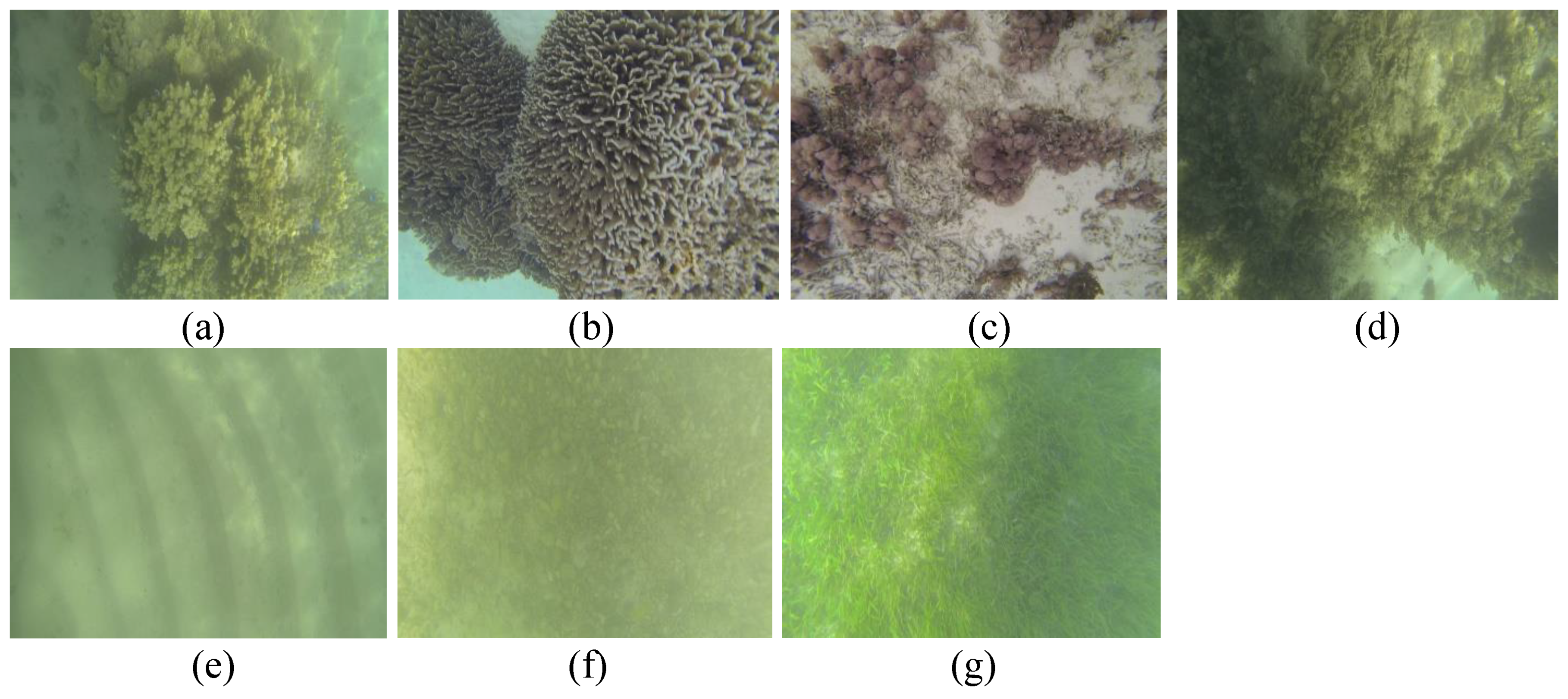
Figure 3.
Various examples of still seafloor images obtained with a GoPro Hero 3 towed video camera for each habitat class over the Shiraho study area: (a) corals, (b) blue corals, (c) brown algae, (d) algae, (e) soft sand, (f) hard sediments, and (g) seagrass.
Figure 3.
Various examples of still seafloor images obtained with a GoPro Hero 3 towed video camera for each habitat class over the Shiraho study area: (a) corals, (b) blue corals, (c) brown algae, (d) algae, (e) soft sand, (f) hard sediments, and (g) seagrass.

Figure 4.
The workflow of the proposed benthic cover classification and 3D mapping.

Figure 5.
Samples of the correct (green) and misclassified (red) benthic cover images over the Shiraho area.
Figure 5.
Samples of the correct (green) and misclassified (red) benthic cover images over the Shiraho area.

Figure 6.
The number of the correct spices classified by each classifier for benthic cover mapping.

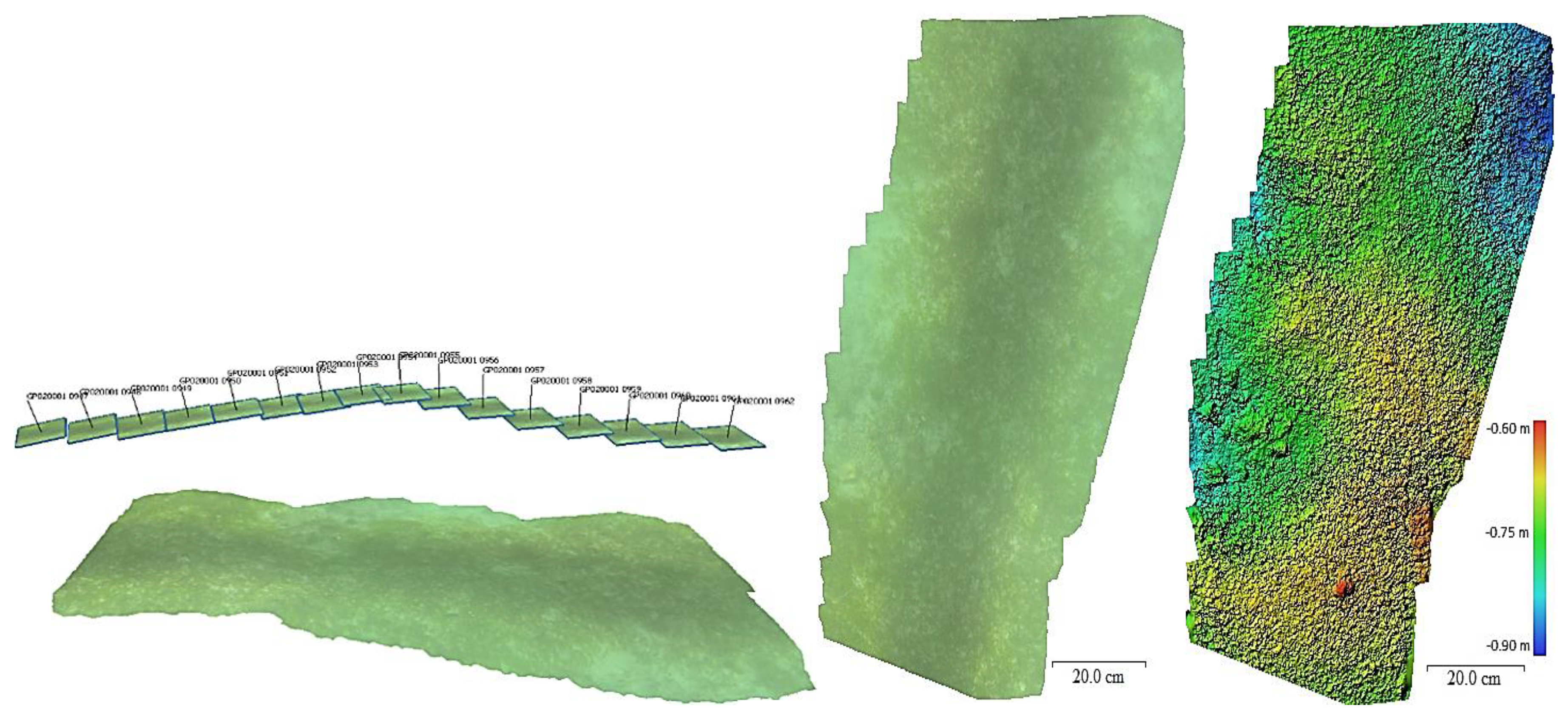
Figure 7.
3D perspective view, orthophoto mosaic, and digital terrain model (DTM) for a categorized algae sample.
Figure 7.
3D perspective view, orthophoto mosaic, and digital terrain model (DTM) for a categorized algae sample.

Figure 8.
3D perspective view, orthophoto mosaic, and DTM for a categorized brown algae sample.

Figure 9.
3D perspective view, orthophoto mosaic, and DTM for a categorized coral sample.

Figure 10.
3D perspective view, orthophoto mosaic, and DTM for a categorized blue coral sample.

Figure 11.
3D perspective view, orthophoto mosaic, and DTM for a categorized seagrass sample.


Table 1.
The selected attributes for the benthic habitat classification process.
| Descriptor | Selected Attributes |
|---|---|
| Texture Parameters | 26 Gray Level Co-occurrence Matrix (GLCM) parameters, including energy, entropy, contrast, correlation, homogeneity, cluster prominence, cluster shade, dissimilarity, image mean, image standard deviation, image mean variance, etc. |
| BOF | A total of 250 attributes extracted from each input image with a 16 grid step, 32 block width, 80% as the strongest feature percent kept from each category, and the grid point selection method for the feature point location selection |
| HSV | A total of 256 HSV values were extracted for each input image |
Table 2.
The overall accuracy (OA) and Kappa results of all methods for benthic habitat classification for Shiraho area.
Table 2.
The overall accuracy (OA) and Kappa results of all methods for benthic habitat classification for Shiraho area.
| Methodology | BAG | K-NN | SVM | FMV |
|---|---|---|---|---|
| OA % | 85.6 | 86.5 | 89.7 | 93.5 |
| Kappa | 0.82 | 0.83 | 0.87 | 0.92 |
Table 3.
The confusion matrix for benthic habitat classification using the fuzzy majority voting (FMV) method.
Table 3.
The confusion matrix for benthic habitat classification using the fuzzy majority voting (FMV) method.
| Classification Data | Reference Data | Row. Total | UA | ||||||
|---|---|---|---|---|---|---|---|---|---|
| A | Br A | Cor | Bl Cor | Sed | SS | Seag | |||
| A | 133 | 1 | 2 | 2 | 0 | 0 | 0 | 138 | 0.96 |
| Br A | 1 | 48 | 0 | 5 | 0 | 0 | 0 | 54 | 0.89 |
| Cor | 1 | 0 | 137 | 10 | 0 | 0 | 0 | 148 | 0.93 |
| Bl Cor | 1 | 1 | 2 | 24 | 0 | 0 | 0 | 28 | 0.86 |
| Sed | 0 | 0 | 0 | 1 | 137 | 14 | 2 | 154 | 0.89 |
| SS | 0 | 0 | 0 | 0 | 1 | 36 | 0 | 37 | 1.00 |
| Seag | 2 | 0 | 1 | 3 | 0 | 0 | 185 | 191 | 0.97 |
| Col. Total | 138 | 50 | 142 | 45 | 138 | 50 | 187 | OA = 93.5% | |
| PA | 0.96 | 0.96 | 0.96 | 0.53 | 0.99 | 0.72 | 0.99 | Kappa val. = 0.92 | |
Key to the benthic habitats names: A = Algae, Br A = Brown Algae, Cor = Corals, Bl Cor = Blue Corals, Sed = Sediments, SS = Soft Sand, and Seag = Seagrass.
© 2020 by the authors. Licensee MDPI, Basel, Switzerland. This article is an open access article distributed under the terms and conditions of the Creative Commons Attribution (CC BY) license (http://creativecommons.org/licenses/by/4.0/).
Share and Cite
MDPI and ACS Style
Mohamed, H.; Nadaoka, K.; Nakamura, T. Towards Benthic Habitat 3D Mapping Using Machine Learning Algorithms and Structures from Motion Photogrammetry. Remote Sens. 2020, 12, 127. https://0-doi-org.brum.beds.ac.uk/10.3390/rs12010127
AMA Style
Mohamed H, Nadaoka K, Nakamura T. Towards Benthic Habitat 3D Mapping Using Machine Learning Algorithms and Structures from Motion Photogrammetry. Remote Sensing. 2020; 12(1):127. https://0-doi-org.brum.beds.ac.uk/10.3390/rs12010127
Chicago/Turabian StyleMohamed, Hassan, Kazuo Nadaoka, and Takashi Nakamura. 2020. "Towards Benthic Habitat 3D Mapping Using Machine Learning Algorithms and Structures from Motion Photogrammetry" Remote Sensing 12, no. 1: 127. https://0-doi-org.brum.beds.ac.uk/10.3390/rs12010127
Note that from the first issue of 2016, this journal uses article numbers instead of page numbers. See further details here.