Biomass and Crop Height Estimation of Different Crops Using UAV-Based Lidar


Wageningen University & Research, Laboratory of Geo-Information Science and Remote Sensing, Droevendaalsesteeg 3, 6708 PB Wageningen, The Netherlands
*
Author to whom correspondence should be addressed.
Remote Sens. 2020, 12(1), 17; https://0-doi-org.brum.beds.ac.uk/10.3390/rs12010017
Submission received: 27 September 2019
/
Revised: 16 December 2019
/
Accepted: 17 December 2019
/
Published: 18 December 2019
(This article belongs to the Special Issue Remote Sensing in Agriculture: State-of-the-Art)
Abstract
:Phenotyping of crops is important due to increasing pressure on food production. Therefore, an accurate estimation of biomass during the growing season can be important to optimize the yield. The potential of data acquisition by UAV-LiDAR to estimate fresh biomass and crop height was investigated for three different crops (potato, sugar beet, and winter wheat) grown in Wageningen (The Netherlands) from June to August 2018. Biomass was estimated using the 3DPI algorithm, while crop height was estimated using the mean height of a variable number of highest points for each m2. The 3DPI algorithm proved to estimate biomass well for sugar beet (R2 = 0.68, RMSE = 17.47 g/m2) and winter wheat (R2 = 0.82, RMSE = 13.94 g/m2). Also, the height estimates worked well for sugar beet (R2 = 0.70, RMSE = 7.4 cm) and wheat (R2 = 0.78, RMSE = 3.4 cm). However, for potato both plant height (R2 = 0.50, RMSE = 12 cm) and biomass estimation (R2 = 0.24, RMSE = 22.09 g/m2), it proved to be less reliable due to the complex canopy structure and the ridges on which potatoes are grown. In general, for accurate biomass and crop height estimates using those algorithms, the flight conditions (altitude, speed, location of flight lines) should be comparable to the settings for which the models are calibrated since changing conditions do influence the estimated biomass and crop height strongly.
1. Introduction
Phenotyping of crops is important to estimate biomass and the potential yield of new varieties of agricultural crops. Due to the increasing need to increase food production and improve the associated quality, it is important to optimize the yield, for which accurate estimation of biomass during the growing season is needed. In this context, phenotyping focuses on the characterization of morphological as well as physiological crop traits. Morphological parameters, such as plant height, stem diameter, leaf area or leaf area index (LAI), leaf angle, stalk length, and in-plant space [1], can be determined with LiDAR (light detection and ranging). Research on phenotyping using LiDAR often focusses on one specific crop, for example, wheat [2,3] or cotton [4].
Phenotyping of individual plants can be done in very high detail with LiDAR, analyzing complex phenotypical properties, such as leaf area, leaf width, and leaf angle [5,6]. For this, plants were put on a slowly turning platform while a fixed LiDAR instrument was used. A drawback of this setup is the low throughput of the scanning system while there is also a need to evaluate phenotypes under field conditions.
For high-throughput phenotyping, traits such as plant-height, LAI, and leaf cover fraction are determined directly in the field, using a LiDAR-based system mounted on a vehicle or RGB cameras mounted on a UAV (unmanned aerial vehicle) [3,4,7]. Tractor based LiDAR systems data have shown good correlation with in situ field measurements of plant height. Sun et al. [4] published an R2 of 0.98 for cotton plants, [2] published an R2 of 0.99 for wheat, and [7] showed an R2 of 0.90 for wheat. These studies show the capability of LiDAR to measure basic phenotypes such as plant height. However, LiDAR systems mounted on tractors can be unsuitable for labour-intensive crops such as rice or in orchards [8], for example, due to compaction of the soil [9]. A UAV equipped with a LiDAR system can overcome those limitations.
Earlier research on the relation between plant height and biomass was based on varying approaches for plant height measurements. Madec et al. [7] found an R2 of 0.88 for the correlation between plant height and field-measured biomass, using a tractor based LiDAR system. Bendig et al. [10] used a structure from a motion (SfM) technique on UAV acquired imagery to derive plant height and found an R2 of 0.81 between field-measured height and SfM derived height.
In the last few years, LiDAR systems have been miniaturized, resulting in lower weights and reduced dimensions, and as a result, can be operated from UAVs. This development opens the way towards high throughput derived, more complex products like biomass and yield, thus, improving the speed and frequency at which these plant traits can be acquired in the field in an undisturbed way.
LiDAR-based biomass estimates of agricultural crops can be derived in different ways. Based on the Lambert-Beer LAI model of [11], the authors of [2] developed a biomass prediction model called the 3-Dimensional Profile Index (3DPI). Where the LIDAR 3D point cloud is divided into layers and for each layer, the fraction of points divided by the total amount of points is calculated. These layers are then summed, and the 3DPI values can be related to biomass with a linear function. As follow up [2] also proposed a voxel-based method (3DVI) to estimate the biomass of wheat. The 3DVI method divides the LIDAR 3D point cloud in voxels of equal size and calculates the ratio between the number of voxels containing points and the number of subdivisions in the horizontal plane. They showed that 3DVI could estimate wheat biomass accurately with an R2 of 0.91, and for 3DPI, an R2 of 0.93 was achieved. Jimenez et al. [2] used a tractor based LiDAR system. An alternative approach using airborne LiDAR was proposed by [12], who used Pearson’s correlation analysis and structural equation modelling (SEM) to estimate plant height and LAI, which proved to be the best predictors of the biomass of maize (R2 of 0.87).
The goal of this study was to investigate the potential of UAV-LiDAR for estimation of crop height and fresh weight biomass for three different agricultural crops. For this, the RIEGL RiCOPTER with a VUX-SYS LiDAR system was flown over fields with sugar beet, wheat, and potatoes, on a number of moments during the growing season. First, it was investigated how accurate this system can estimate crop height and biomass. Next, we answered the question if it is possible to create models that are generally applicable for different crops. Finally, we did experiments with different UAV flight patterns, altitudes, and speeds to investigate if this influences the LiDAR-derived plant height and biomass estimation. Optimization of the flight parameters was beyond the scope of this paper.
2. Materials and Methods
2.1. Study Area
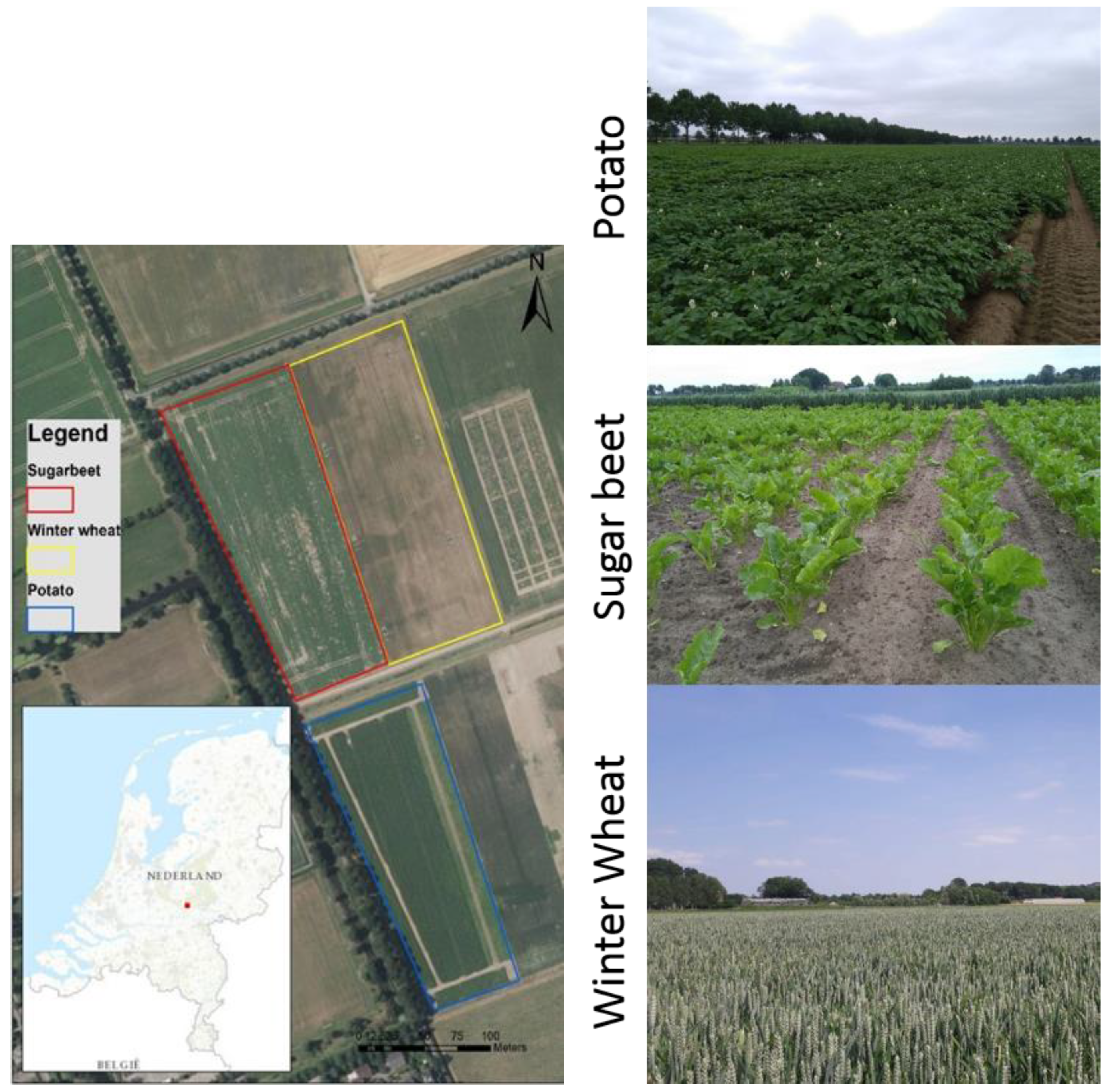
Three fields with different crops, each covering approximately 2 ha, were selected at the experimental farm of Wageningen University, located just north of Wageningen in the Netherlands (Figure 1). The three types of arable crops in this study are sugar beet, winter wheat, and potatoes (Table 1), which were planted on a Placic Podzol [13]. The variation in elevation in the fields is very small with a height difference of less than 10 cm going from east to west in the area. Orientation of the main crop rows for all three crops is north–south. The plant density of winter wheat was 260 plants/m2. Planting distance for potato and sugar beet was 30 cm and 23 cm, respectively.
2.2. Data Acquisition
UAV-LiDAR data and field measurements of crop height and biomass were collected simultaneously on four dates (Table 2). For the 1st, 2nd, and 4th flight date, field data were collected on the same day, directly starting after the flight and finished within 3 to 4 hours. The 3rd flight day was not planned initially, so no field measurements were done on that day, but this flight was conducted only 2 days after the 2nd flight. Therefore, the field data collected at the day of the 2nd flight were used for both those flights.
2.2.1. Field Data Collection
Plant height was measured using a ruler at 14–21 locations in each field. Locations were chosen in such a way that differences within the field were well represented. On each location, an average height was calculated based on three height measurements of randomly selected plants taken within 15 cm of each other. Biomass was determined through destructive sampling at different locations within the field, differing from the plant height sampling locations [14]. For potato and sugar beet, five biomass samples per field were taken and for winter wheat three. Biomass was harvested after the flights. Biomass samples were taken for the first, second, and fourth flight day only, which resulted in 15 samples for both potato and sugar beet and 9 samples for winter wheat. For potato, biomass was harvested for one meter along the potato ridge and converted to biomass per 1 m2. The same procedure was used for harvesting the sugar beet, where one meter in the planting direction was harvested and converted to biomass per 1 m2. For wheat, an area of 1 m2 area was harvested. Biomass was measured as fresh biomass weight directly after harvesting. Table 3 shows the mean and standard deviation of every field campaign. The location of every crop trait measurement was measured with a Topcon HIPER V RTK-GNSS system (TOPCON, Japan), which has a sub centimeter accuracy.
2.2.2. UAV-LiDAR Data
LiDAR data were collected using the RIEGL RiCOPTER UAV system (Riegl, Austria) with the VUX-SYS laser scanner mounted underneath. The authors of [15] provided a description of the details of the system. The VUX LiDAR unit has an accuracy of 1 cm and precision of 0.5 cm. The absolute positioning error on the ground also depends on the IMU accuracy, which was <5 cm in the horizontal and <10 cm in vertical direction. Analysis of previous datasets acquired with the same setup resulted in positioning errors of <5 cm. The scanner pulse repetition rate was set at 550 kHz, the scanner angle from 30–330 degrees, and the scanner speeds were synchronized with the UAV forward speed to create a regular point spacing. On the predefined dates, UAV-LiDAR data was acquired by flying at 40 m above ground level (m.a.g.l.) with a programmed speed of 6 m/s. The actual flight altitude and speed can deviate slightly from those preset values and were calculated from the flight recordings afterwards (Table 4: mean flying height and speed).
Further, to assess the influence of the flying height and speed on the accuracy of acquired phenological parameters, additional flights were done within a few days after the second flight day, with heights varying from 20 to 90 m above ground level, and with programmed speeds ranging from 3 m/s to 8 m/s. An overview of the flights and the actual flight data is shown in Table 4. The code given in Table 4 is later used to identify the data acquired from each flight.
If during the analysis it appeared that field measurements of plant height or biomass ended up in the same pixel as a driving path as seen from the Lidar 3D point cloud, the point was moved 1 pixel away from the driving path. This was the case for one point in the winter wheat dataset. Further, the field measurement locations were selected before the flights were made. Points that appeared to be in areas with a much lower LiDAR point density were excluded from the height and biomass analysis. Two winter wheat points during the last flight date had to be excluded for this reason.
2.3. Data Pre-Processing
Riegl RiCOPTER data was pre-processed to co-registered point cloud datasets (Figure 2) using the standard Riegl processing chain as outlined by Brede et al. [15]. This includes trajectory processing, for which a virtual GNSS base station was used. The movements of the UAV platform were corrected using the POSPac software (Applanix, Canada), which combines the GNSS correction and the movement data recorded by the IMU, with a reported precision of ~1–2 cm for all flights. To produce a geo-referenced point cloud, the flight path, and raw point cloud data were combined in RiPROCESS (Riegl, Austria). Further refinement of the point cloud, using automatically detected surfaces, was done by RiPRECISION (Riegl, Austria). The final co-registered and geo-referenced point cloud datasets were stored in LAS format.
The point clouds were clipped for the boundaries of the three fields (Figure 1). The ground points were selected using LasTools (Rapidlasso, USA) with the lasground function. From the points classified as ground, a triangulated irregular network (TIN) was created. The height of each non-ground classified point was calculated as the height above this TIN, using the “replace z” option in lasground. The same procedure was applied for all the three fields.
2.4. Data Analysis
2.4.1. LiDAR Based Plant Height
Due to the difference in the structure of the crop canopies, the highest point in the point cloud is not always the best representation for the field-measured crop height. Therefore, for each grid cell of 1 m2 the average plant height was derived by including a certain number of top-of canopy points. To determine the amount of top-of-canopy points needed to get the best plant height estimation, a theory was used that is more commonly used in economics to decide on the best allocation of products: the Pareto efficiency score [16]. This method compares different alternatives and based on preset criteria, calculates a score of optimal performance. In this case, we used this method here to decide based on two criteria, namely the highest R2 and lowest root mean squared error (RMSE), which are calculated for each alternative of measured plant height and a certain number of top-of canopy points. The method then only selects the combination for which no better combination exists. This can result in multiple optimal Pareto efficiency scores. Next, from these Pareto efficient combinations, the combination with the highest R2 is selected. This was done once for the whole growing season for every crop. The corresponding number of top-of canopy points of this combination was used to calculate the plant height of each raster cell within the field. A linear model relating field plant height measurements to LiDAR-derived plant height was built using the 3D LiDAR point cloud by taking the optimal number of top-of-canopy points into account.
2.4.2. Crop Biomass
To estimate biomass from the LiDAR point cloud, the 3DPI method as developed by the authors of [2] and described by Equation (1) was used and calculated for a cell size of 1 m2:
where i is a given 10 mm vertical layer with 0 being the ground layer and n the uppermost layer respectively; k is a tuning parameter changing from −1 to 5 by steps of 0.05; pi is the number of LiDAR points for a given layer of 50 mm; pt is the total number of LiDAR points for all layers; and pcs is the cumulative sum of LiDAR points intercepted above a given layer of 50 mm, as described in [2].
To derive the biomass prediction model, a linear regression was performed between the dimensionless 3DPI indicator and the biomass measured in the field based on the 3DPI indicator. First, the optimal value for the parameter k was determined. For each individual crop and flight, the 3DPI score was calculated by varying the k-parameter from −1 to 5 by increments of 0.05. The best k-parameter was chosen based on the correlation between the field measurements and the 3DPI score. The data for each crop was combined into a crop-specific seasonal prediction model for the flights Day1-MA-MS, Day2-MA-MS, and DAY4-MA-MS. Secondly, all the data of these flights and crops were combined into a general non-crop-specific seasonal prediction model.
Next, the flight data from DAY2-LA-MS, DAY2-LA-LS, DAY3-HA-HS, and DAY3-LA-LS were used to determine the effects of different flight specification and were compared to Day2-MA-MS. The 3DPI for these four flights was calculated using the same field measurements of plant height and biomass as for Day2-MA-MS. This enabled the analysis of different flight settings because only the 3DPI indicator differed between the flights so a direct comparison can be made. To visualize the differences between these four flights, maps of predicted biomass were derived and difference maps of each flight with flight Day2-MA-MS were calculated.
2.4.3. Model Validation
To assess the performance of the models (Figure 2) for determining biomass, plant height, and the general models, three statistical indicators were used; the coefficient of determination (R2), the mean absolute error (MAE), and the RMSE. We included a cross validated MAE and RMSE, using a k-fold cross validation. For each k-fold, the out-sample RMSE and MAE were calculated, after which they were averaged over the n-number of k-folds used in the cross validation. These averaged out-sample RMSE and MAE were compared to the in-sample RMSE and MAE. This comparison shows the predictive power of the model (out-sample errors).
For the plant height analysis, a 10-fold cross validation was performed, using 61, 51, and 51 samples for potato, sugar beet, and wheat, respectively (Table 3). For the biomass estimation, a repeated 5 × 3-fold cross validation was performed. The reason for this repeated cross validation for biomass is the limited amount of biomass samples available for the statistical analysis. In this case, we used 15, 15, and 9 samples for potato, sugar beet, and wheat, respectively (Table 3).
For the biomass error analysis, the MAE and RMSE were then normalized by dividing by Xmax-Xmin, where Xmax is the highest measured biomass sample in the dataset and Xmin the lowest measured biomass sample in the dataset, resulting in a normalized mean absolute error (NMAE) and normalized RMSE (NRMSE).
3. Results
3.1. Crop Specific Models
3.1.1. Plant Height
Based on the analysis of the Pareto efficiency scores, the LiDAR plant height for each grid cell of 1 m2 is based on the top 10 points for potato, on the top 90 points for sugar beet, and for winter wheat on the top 30 points. The average height of these points serves as the LiDAR-based plant height estimation.
The correlation between field-measured height and LiDAR-based plant height is highest for sugar beet and winter wheat (Figure 3). Plant height was most accurately derived for winter wheat with an RMSE of 3.4 cm. Determining plant height for potato proved to be the most difficult, showing relatively large residuals.
Figure 3 shows that there is a general over prediction of plant height for potato while winter wheat shows an underestimation. As winter wheat has a relatively open and erectophile structure, the number of returns in the top of the canopy could be lower, resulting in an underestimation of height. Although sugar beet falls on the 1:1 line, the prediction of plant height has a higher spread than winter wheat, which is shown by the larger MAE and RMSE. The over prediction of potato is most likely the result of the complex canopy, which is explained in more detail in the discussion.
3.1.2. Biomass
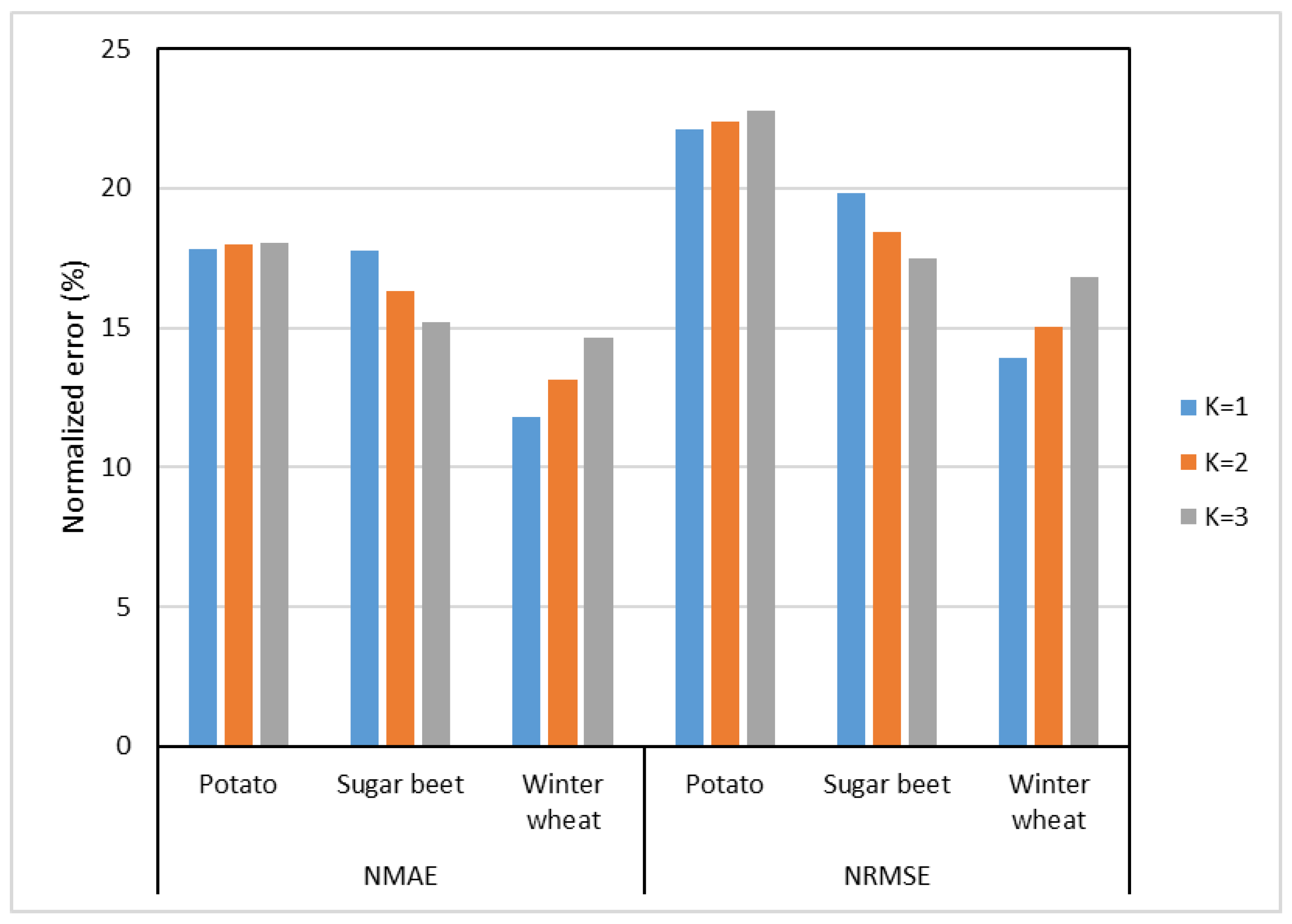
Choosing k = 1 for potato and winter wheat and k = 3 for sugar beet results in the best fit for the biomass models. Values lower than k = 1 proved to be very unstable in the performance for the 3DPI algorithm, showing large fluctuation in R2 values. Values higher than k = 3 became saturated and showed only minor increases in R2. For potato and winter wheat the model errors, NMAE and NRMSE are the smallest for k = 1 (Figure 4), while for sugar beets the errors are smallest for k = 3.
Potato shows a relatively large difference between the NMAE and NRMSE compared to those of sugar beet and winter wheat. This indicates that the low R2 is most likely the result of large residuals (Figure 4). Furthermore, the spread in points for potato is less equally distributed between large and small residuals compared to the spread of points for sugar beet and winter wheat (Figure 5). This explains the larger NRMSE and NMAE of potato.
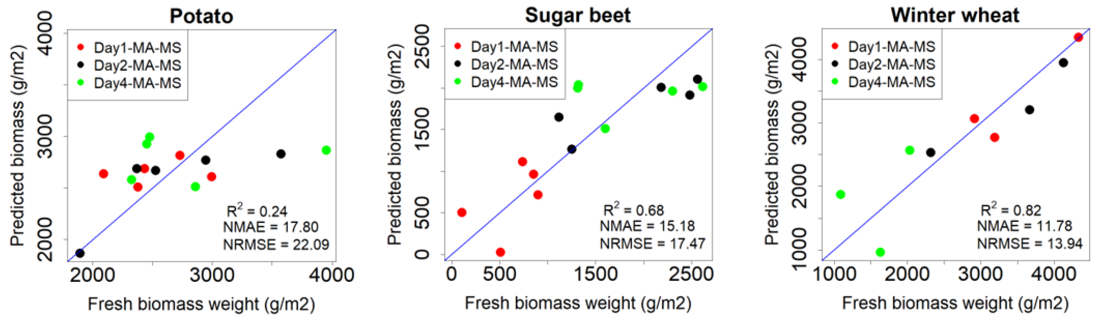
The prediction model for potato does not provide reliable estimates of biomass, especially for values higher than 3500 g/m2 (Figure 5) in which biomass is underestimated. Furthermore, the scatterplot does not show a strong relation. For sugar beet, there is a good correspondence between the fresh biomass in the field and the LiDAR predicted biomass (Figure 5). Also, the crop development during the growing season is captured well: during flight 1, the sugar beets were still small, and the field was only partially covered, while during flights 2 and 4 the sugar beets had grown, which is also derived from the UAV-LiDAR observations.
The biomass of winter wheat was determined most accurately. For flights 1 and 2, the points are practically on the 1:1 line (Figure 5). During the 4th flight, the wheat had ripened, which lowered the amount of fresh biomass.
3.2. General Prediction Models
3.2.1. Crop Height
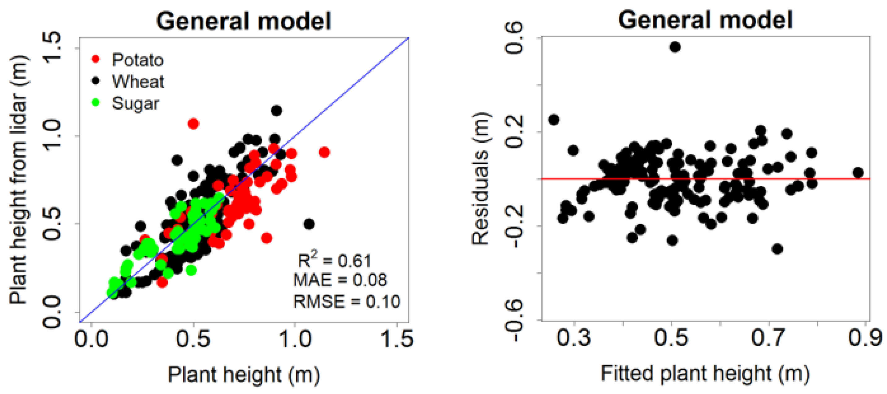
When combining the crops into a general prediction model for plant height, the RMSE is 10.1 cm (Figure 6). This error is much larger compared to the crop-specific models. For example, this accuracy was 3.4 cm for winter wheat in the single crop model (Figure 3).
The Pareto method is used to determine the optimized number of points to be used to calculate the height per pixel, which showed that using 100 points per pixel yielded the best fit for the general model, resulting in an R2 of 0.61 for the general model. This is lower than the R2 for sugar beet and winter wheat (0.70 and 0.78, respectively), but higher than that of potato (0.49). The residual plot shows a random distribution of points with one outlier (Figure 6). This point comes from the potato dataset, but no valid reason was found to exclude the point.
3.2.2. Biomass
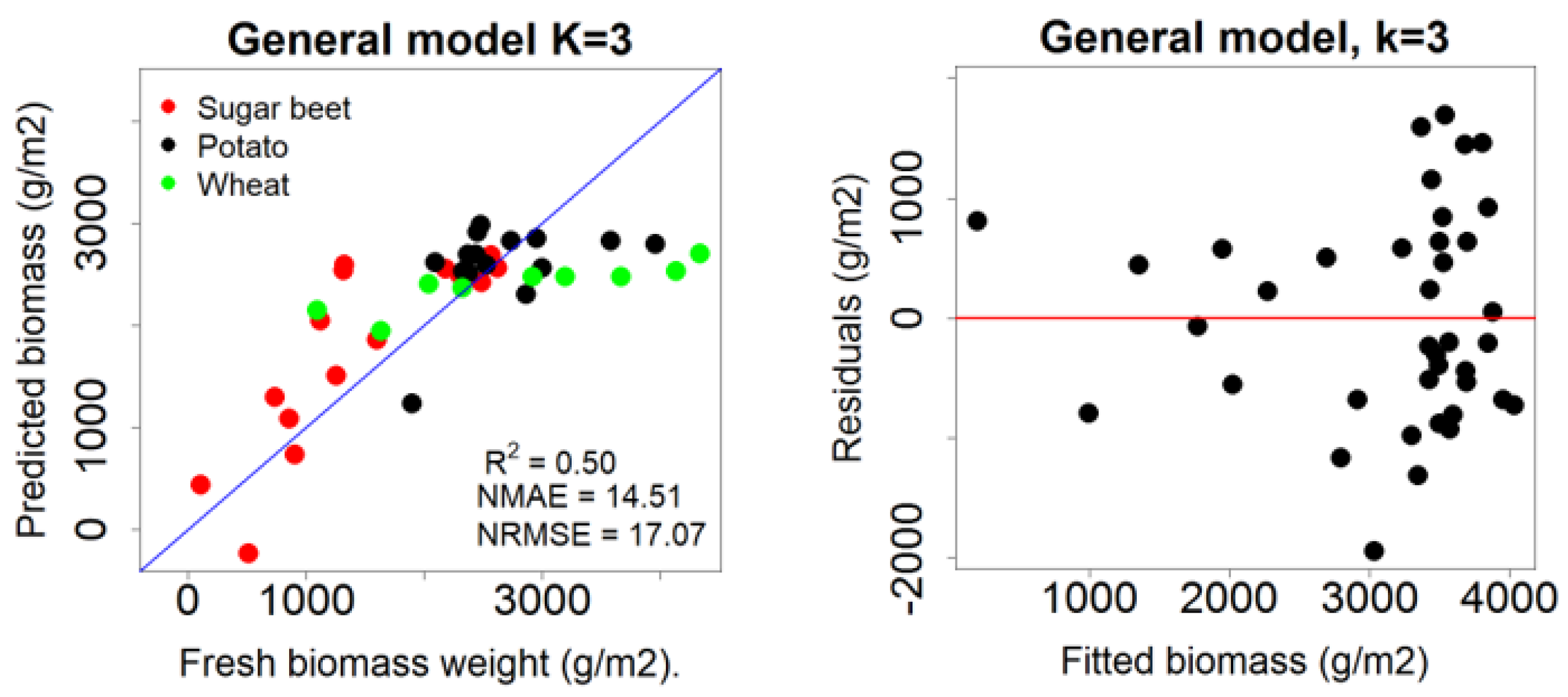
The general model for biomass performed worse for biomass prediction of winter wheat; the normalized error increased to 17.07% for the general model compared to 13.9% for the crop-specific model (Figure 7) based on tuning-parameter k = 3. The general models were fitted using different k-factors, where the R2 was 0.47 for k = 1, 0.49 for k = 2 and 0.50 for k = 3. The generic model saturates for higher biomass predictions, especially for winter wheat (Figure 7). This indicates that a new model should be built for the higher biomass estimates. However, the general model can be used to predict biomass for potatoes (NRMSE = 22.1%) and sugar beet (NRMSE = 17.47%), in which NRMSE values are larger than those of the general model (NRMSE = 17.07%).
The cross validated NRMSE shows that biomass can be predicted on a new dataset with an NRMSE_cv of 17.61%. The NRMSE_cv is 0.54 larger than the NRMSE for k = 3. This indicates that the model could be used for fields, where no biomass samples were taken for calibration.
3.3. Influence of Flight Characteristics on Plant Height
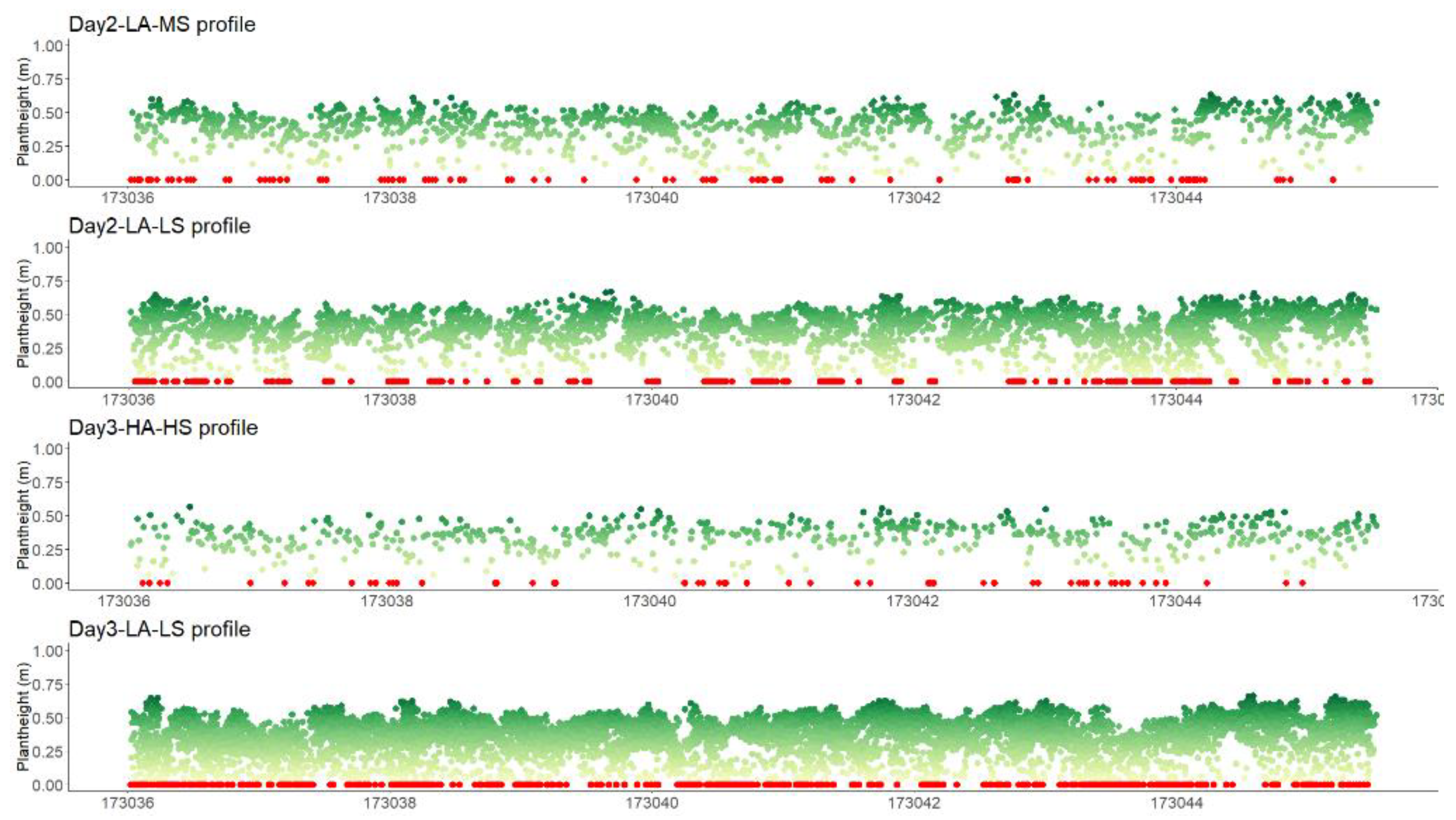
Changes in flight characteristics (altitude and speed) result in differences in point cloud density (Figure 8), where a cross section (10 × 0.2 m) of the sugar beet point clouds of four flights with different flight characteristics are shown. The flights were done on two days, with one day in between, but we assumed that the crops did not change between those two days.
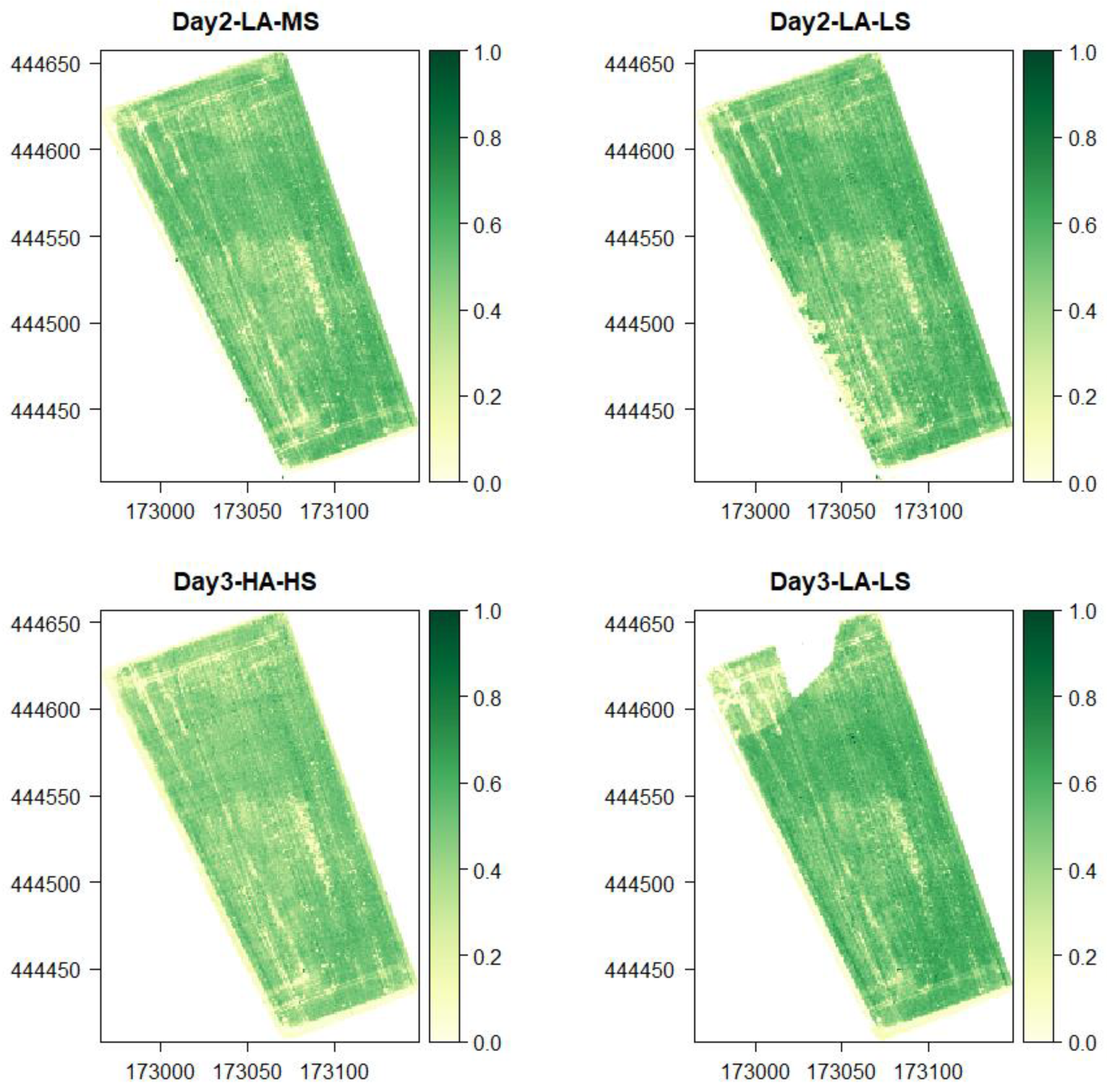
Measured plant height is consistent for the different flight characteristics, except for the high and fast flight (DAY3-HA-HS: 90 m, 8 m/s). As can be seen in Figure 8, this results in a much lower point density and an underestimation of the crop height, shown by the lighter green colours in Figure 9. However, the spatial patterns of crop height between the four sets of flight characteristics are comparable. The locations with low and high crop height show a comparable location and distribution. For DAY3-LA-LS height map, the north-western corner of the field was not covered well by the pre-programmed flight path, which resulted in a lower point density and, thus, an underestimation of crop height. This indicates that the flight characteristics do not influence the spatial patterns of estimated crop height, but it is important to keep them consistent for measuring temporal changes in crop height.
3.4. Influence of Flight Characteristics on Biomass
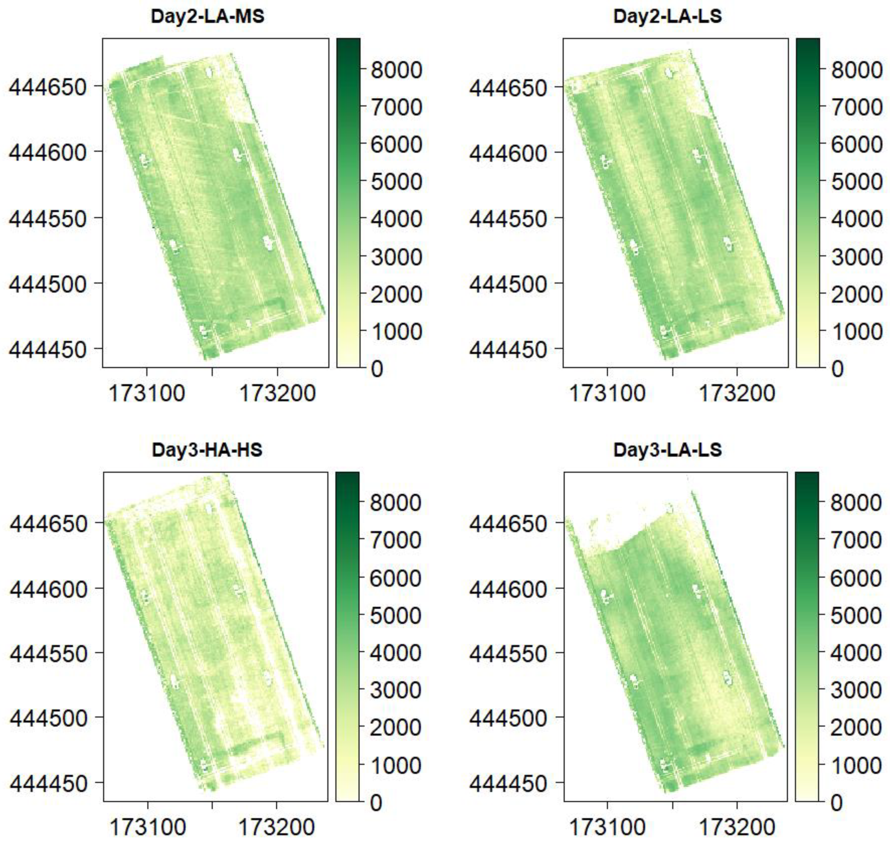
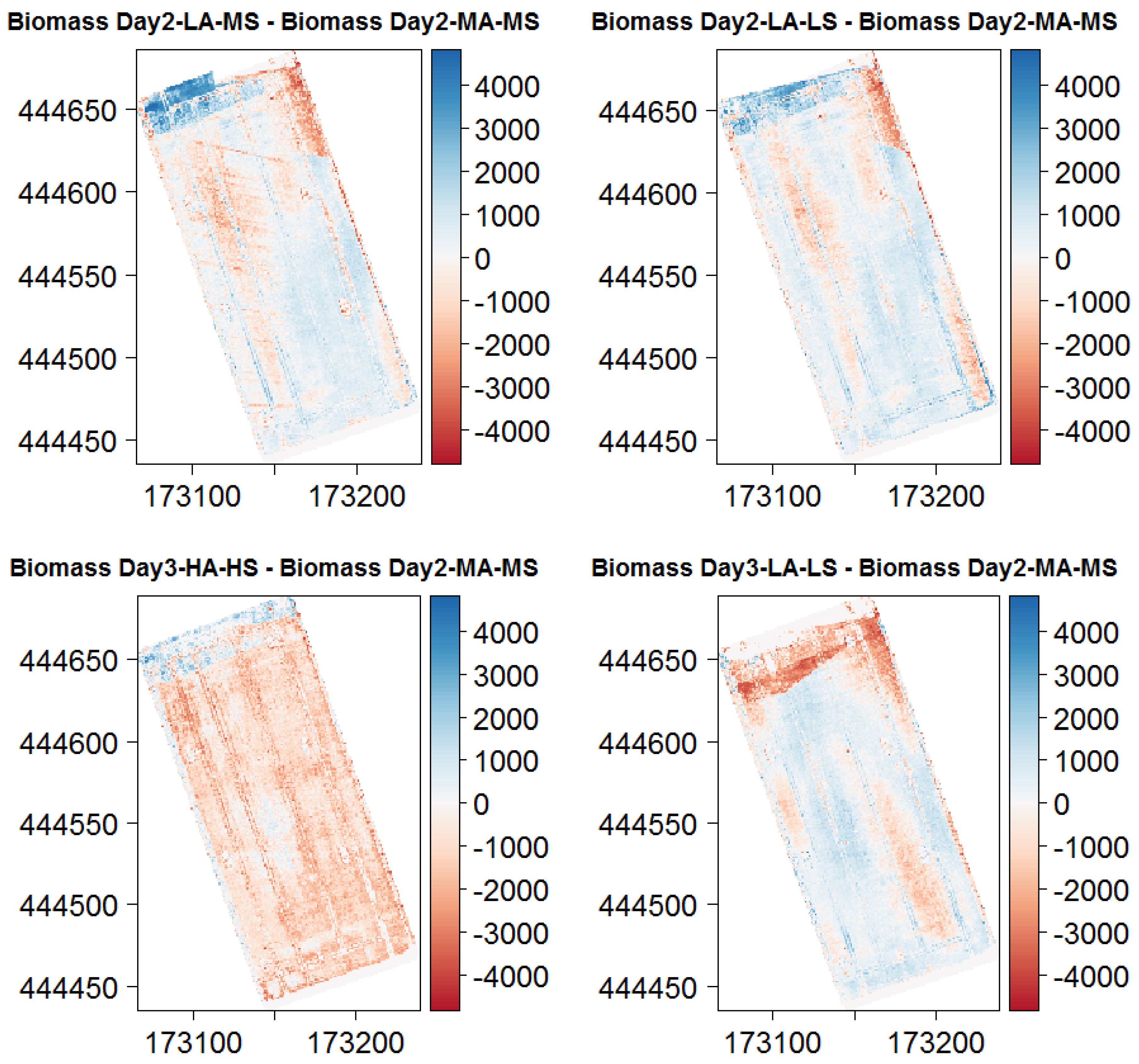
Biomass maps based on the 3DPI scores show varying patterns of biomass, dependent on the flight characteristics (Figure 10). The absolute differences, compared to flight Day2-MA-MS (40 m, 6 m/s), are more clearly visible in Figure 10. Flying higher and faster (DAY3-HA-HS), results in an underestimation of the amount of biomass. For flight DAY3-HA-HS, the average biomass estimation was 1622.1 g/m2, where for Day2-MA-MS, the average biomass estimation was 2479.7 g/m2 (Table 5). For the other flight characteristics, the overall estimate of biomass does not deviate too much from the standard flight settings, but there are locations where the estimated biomass for the adapted flights is lower compared to the standard flight. Further investigations learned that those areas are located exactly between two flight lines. It is important to indicate that the exact position of the flight lines was not consistent for the different flights. For each of the flights with the standard settings, the same pre-programmed flight paths were used, but for the flights with adapted altitude and speed, new flight plans were made, resulting in different flight patterns. This results in a different point density and point distribution along the dataset, which appears to influence the estimated biomass more than the altitude and speed.
The biomass prediction for flight Day3-HA-HS shows an under prediction compared to the other flights (Table 5), where for plant height the difference in the mean between the flights are smaller. The sugar beet plant height estimation shows almost no variation between the flight characteristics describing the field data from 29 June 2018. The biomass estimations for winter wheat does appear to be sensitive to a difference in flight characteristics. There are large differences in the mean prediction between the different flight specifications, where for faster and higher flights (Figure 11 and Table 5: DAY3-HA-HS), an under prediction of biomass occurs compared to flight Day2-MA-MS.
4. Discussion
4.1. Plant Height
Depending on the type of crop, the accuracy for plant height retrieval varied between 3.4 cm for winter wheat, 7.4 cm for sugar beet, and 12 cm for potato (Figure 3). Previous research efforts on determining plant height via LiDAR have focused on winter wheat, where Jimenez-Berni et al. [2] found an accuracy of 1.7 cm for a ground-based LiDAR system. Madec et al. [7] compared plant height derived from a LiDAR scanner on a ground vehicle with estimates from SfM analysis on RGB-UAV images. The latter method provided an accuracy of 3.47 cm for winter wheat plant height, proving that the methodology presented within this paper proves just as accurate. Homan et al. [17] showed that using a terrestrial laser scanner (TLS), the RMSE was 2.7 cm for wheat, which is comparable to the achieved accuracy by the RiEGL RiCOPTER UAV LiDAR system. This, and previous research, shows that using a UAV-based LiDAR system can be used to accurately assess plant height for winter wheat fields.
However, the accuracy drops for crops with a more complicated canopy structure, such as potato and sugar beet, where it proves to be harder to provide a plant height estimate with high accuracy. This starts with the procedure for field measurements. Winter wheat is an easy-to-measure crop in the field due to its erectophile structure and a homogeneous pattern in height. Potato and sugar beet and their planophile leaf angle distribution prove to be harder to measure within the field, which is further complicated for potatoes since it is grown on ridges. Therefore, it is visually harder to determine the highest point of a specific location. We tried to account for this by averaging field measurements over the three highest points in close proximity, but we cannot ignore the fact that there are uncertainties in the field measurements (Table 3).
In particular, potato proved to be a difficult crop because it grows on ridges, showing the need for a good digital terrain model (DTM) of these ridges. A flight should be performed just after planting the potato to get a good DTM, which can be used to normalize the 3D LIDAR point cloud of the flights further during the growing season. This research started when the potato plants were already developed, resulting in a closed canopy, making it impossible to create a good DTM. This could be one of the reasons for the worse performance of potato height estimation.
As a result, the standard deviations for potato are generally larger than for the other two crops (Table 3). Especially on 25 June when the potato plants were fully grown, it proved more difficult to get accurate measurements.
4.2. Biomass
The 3DPI algorithm proved to estimate the biomass of winter wheat (NRMSE = 13.9% and R2 = 0.82) and sugar beet (NRMSE = 17.47% and R2 = 0.68) well, showing slightly higher accuracies compared to the paper of [2], where an NRMSE of 19.82% was achieved for winter wheat. It should be noticed that the early growth stages are not included in this study, which partially explains the differences in NRMSE. For winter wheat, similar results were obtained in [18], where a linear relation was also examined between LiDAR-derived plant height and biomass, reporting an R2 of 0.88.
Possible improvements in the amount of biomass for winter wheat could be made using the dry weight of the plant material. Especially during the ripening phase, the water content of winter wheat decreases [19], resulting in a mismatch between the 3DPI algorithm and the measured fresh weight biomass. The 3DPI method is developed on plant structure and does not account for the changing water content within the winter wheat. Also, research by [20] showed that LiDAR laser scans proved to be useful in determining leaf water content. This shows that there is an influence on the return signal, which is influenced by the water content that has not been accounted for now. This effect depends on the architecture, size, and density of the crop and, as such, is crop dependent.
The 3DPI algorithm proved to be unsuitable for estimating the biomass of potato. The 3DPI algorithm was developed for winter wheat and not tested on other crops so far. Probably the main reason is the very dense canopy, resulting in very few points in the lower parts of the canopy, which resulted in a small number of returns lower in the canopy. These points underneath the canopy are needed to create a complete height profile relative to the 30 cm high ridges where potatoes are grown on, resulting in a better representation of the above ground biomass. The reason the algorithm works better for sugar beet, which also shows a relatively dense canopy, is that sugar beet has larger inter-row spacing which leads to more hits from larger scan angles.
The biomass prediction could possibly be improved for areas with a low points density by changing the p_i layer size in the 3DPI algorithm. In this study, a p_i layer size of 50 mm was chosen for two reasons. Firstly, because our point density was lower than of the experiment done by [2], choosing a p_i of 10 mm would result in layers with no points in it. This could possibly influence the 3DPI algorithm negatively. Thus, increasing the p_i layer size resulted in an increase in points per p_i layer, but how this influences the final 3DPI indicator should be further researched. Secondly, choosing a larger p_i resulted in a faster computation time, which was useful for the large files we had.
Possible further research could be done using machine learning, where the 3DPI may be one of many predictors to estimate biomass. Using, for example, a PLS regression as mentioned in [21], or using machine learning approaches like [22], where a deep convolutional network was used to predict biomass using RGB imagery. Or the machine learning approach of [23], where they used a range of spectral indices as predictors to estimate above ground biomass with an NRMSE of 24.95%. Combining these different methodologies with a predictor such as the 3DPI indicator could result in a better prediction of biomass.
4.3. General Models
The accuracy of the prediction of plant height using the general prediction model is 10.1 cm, which is lower than those for the crop-specific prediction models of sugar beet (7.4 cm) and winter wheat (3.4 cm).
The general model for biomass prediction displays a strong influence of sugar beet on the total prediction model (Figure 7). The general model has the best predictive power at k = 3, showing this influence. Sugar beet had the highest predictive power for k = 3, with the other two crops at k = 1 (Figure 5). The reason for this over-representation of sugar beet is due to larger sample size of 15 samples compared to nine for winter wheat and the better performance of the sugar beet biomass model compared to that of potato. Combining these two explains why at k = 3, the model has the highest predictive power. When combining data from different crops, extra attention should be paid to include an equal sample size of the multiple crops. Therefore, using a crop-specific model to estimate crop height from UAV-LiDAR data proves to increase the prediction accuracy. However, depending on the accuracy requirements, a general model could provide plant height estimations with an accuracy of 10.1 cm and a biomass estimation with an accuracy of 17.07%. The results of this research show that crop-specific biomass models have a higher retrieval accuracy; however, further research is required to evaluate if general models can be relevant for mixed cropping systems.
Again, the trade-off is visible between a general biomass model, compared to the specialized models for each individual crop. Furthermore, the model now has to be fitted through three kinds of crops, which are completely different from each other. It was also indicated that different K-values were needed to get a good fit of the specialized biomass models. A certain combination of 3DPI indicator and measured biomass for potato does not necessarily correspond to the same combination of the 3DPI indicator and measured biomass for winter wheat. Therefore, limiting this general applicability of the model, the 3DPI appears to be crop sensitive. Possible other factors, such a height statistics derived from the LiDAR 3D point cloud as analyzed in [21] or the spectral vegetation indices of [23], could be helpful to make the 3DPI method less crop sensitive, which is something for further research.
4.4. Influence of Flight Altitude and Speed on Biomass and Plant Height Estimation
Plant height estimation from 3D points can be accurately achieved when the data is acquired at high speed and relatively high altitude. The LiDAR-derived plant height from DAY3-HA-HS, which was acquired at 92.68 m.a.g.l. and a speed of 7.39 m/s, still shows the same patterns as with DAY2-LA-MS and DAY2-LA-LS, but the general plant height is lower (Figure 9). The LiDAR-derived plant height underestimates the plant height compared to DAY2-LA-MS on average with 4.03 cm. This underestimation is still smaller than the sugar beet plant height model error of 7.2 cm, showing that acquiring plant height could be done with these settings. Therefore, speeding up data collection and covering larger areas is feasible.
Applying the generic model for sugar beet on the 3D points clouds from the flights DAY2-LA-MS, DAY2-LA-LS, DAY3-HA-HS, and DAY3-LA-LS showed that between DAY2-LA-MS, DAY2-LA-LS and DAY3-LA-LS, there is no real difference in LiDAR-derived plant height. This indicates that there is no real benefit in slowing down to 2.53 m/s or decreasing flying height. The different flight specifications do result in different point densities and point distributions. However, this results mostly in more points underneath the canopy, which has only a minor influence on the top of canopy points. To increase accuracy, a DTM could be created before plants start to grow, decreasing the dependence on getting enough returns underneath the canopy.
For biomass estimation, the under the canopy points are important, where for DAY3-HA-HS, a large under estimation is made averaging 858.8 g/m2 compared to the biomass prediction for DAY2-LA-MS. There are not enough points to represent the full height of the plant. The non-normalised accuracy of the winter wheat biomass model was 415.8 g/m2. Showing the inaccuracy of data acquired at 92.68 m.a.g.l. and 7.39 m/s compared to that of DAY2-LA-MS, acquired at 24.16 m.a.g.l. and 4.17 m/s.
Changing flight characteristics shows some areas with patches where the biomass for wheat is underestimated (Figure 10). These patches appear to result from areas that are not covered with any flight lines and almost no perpendicular flight lines. It appears to be crop-specific as these patches do not appear for sugar beet and potato. A possible reason why it affects winter wheat more is that laser pulses from the LiDAR UAV penetrate more easily due to its erectophile leaf structure compared to the planophile leaf structure of potato and sugar beet. Sofonia et al. [24] showed that for a LiDAR-based application, a cross-flight pattern worked best. A better cross pattern and closer flight lines could, therefore, possibly improve biomass estimation in general because laser pulses are acquired from multiple directions increasing the chance of hitting parts of the plant underneath the canopy and remove these unwanted patches. For an accurate biomass prediction, a homogeneous point density is needed.
To allow a good estimation of biomass and crop height over the growing season, it is necessary to keep the flight patterns consistent for all flights. Our results show that biomass and crop height estimation errors increase if the point density and point distribution vary from the circumstances used to calibrate the models. To determine the optimal flight pattern, altitude, and speed, more intensive experiments should be done.
4.5. Outlook
Our results show the possibilities for UAV LiDAR to estimate plant phenotypes, such as biomass and plant height, accurately and with high throughput. This fills the gap between slower but highly accurate tractor-based LiDAR systems and high-throughput but less-detailed manned airborne systems as indicated by [25]. Therefore, providing a solution to situations where a quick analysis of the field is required, tractor-based solutions are not suitable. Furthermore, this study shows that crop trait monitoring can be done throughout the season, using the same model trained on data from the whole season. Moreover, this research showed that under uncontrolled conditions, relevant biomass and plant height estimations can be made, which is marked as a bottleneck in the review paper of [26]. When using UAV-LiDAR for high-throughput estimation of plant height and biomass [27], time should be invested in creating a detailed and structured flight plan. A flight plan would ideally consist of a cross-flight pattern and it will cover the whole field, where flights lines are created alongside the boundaries.
This research furthermore showed that there are limitations to the biomass estimation for certain crops and that models developed for a specific crop cannot directly be used for other crops, and generic models should be used with care. For a fully operational approach, an effort should be made towards combining LiDAR with hyperspectral data, as mentioned by [22,23,26], so models can be trained for a range of crops. This will increase both the accuracy and general applicability of high-throughput biomass estimation models. Also, alternative methods for canopy height determination from UAV-based 3D point cloud datasets have recently been published [28].
5. Conclusions
Retrieval of plant height and biomass using UAV-LiDAR proved to be possible for sugar beet and winter wheat. While for potato both plant height and biomass estimation proved to be hard due to the complex canopy structure and the ridges on which potatoes are grown. For plant height, the data acquisition can be performed relatively fast and at high altitudes increasing opportunities for high-throughput approaches. However, for accurate biomass estimates, the flight conditions (altitude, speed, location of flight lines) should be kept constant. The higher acquisition speed, compared to, for example, tractor-based LiDAR systems, means that UAV-LiDAR can be used to assess large areas and can provide data quickly. Creating a reliable general model to predict biomass for different crops results in a lower accuracy, especially when crops with a dense canopy like potato are included. To increase the predictive performance of both LiDAR-derived plant height and biomass, a clear DTM should be created before germination of the plants. This accurate DTM could then be used to accurately perform the height normalization of the 3D LiDAR point cloud.
Author Contributions
Conceptualization, H.B., L.K., J.t.H.; methodology, H.B., L.K. and J.t.H.; software, H.B., J.t.H.; validation, H.B., L.K., J.t.H.; formal analysis, J.t.H.; investigation, H.B., J.t.H.; resources, L.K.; writing—original draft preparation, J.t.H.; writing—review and editing, H.B., L.K., J.t.H.; visualization, J.t.H.; supervision, H.B., L.K.; project administration, L.K.; funding acquisition, L.K. All authors have read and agreed to the published version of the manuscript.
Funding
The access to the RiCOPTER was made possible by the Shared Research Facilities of Wageningen University & Research. This work was supported by the SPECTORS project (143081), which is funded by the European cooperation program INTERREG Deutschland-Nederland.
Acknowledgments
We would like to acknowledge all the people that assisted with this research, where without them, the field campaign would have taken much longer. Therefore, special thanks to the following persons without whom this research could not be performed. Berry Onderstal for assisting with the biomass sampling. Marcello Novani, Kim Calders, Tessa Rozemuller, Tim Jak, Sophie Stuhler and Hannah Stuhler for assisting in the field campaigns. And Matthijs ten Harkel for correction and editing of the paper manuscript.
Conflicts of Interest
The authors declare no conflict of interest.
References
- Qiu, R.; Wei, S.; Zhang, M.; Li, H.; Sun, H.; Liu, G.; Li, M. Sensors for measuring plant phenotyping: A review. Int. J. Agric. Biol. Eng. 2018, 11, 1–17. [Google Scholar] [CrossRef] [Green Version]
- Jimenez-Berni, J.A.; Deery, D.M.; Rozas-Larraondo, P.; Condon, A.G.; Rebetzke, G.J.; James, R.A.; Bovill, W.D.; Furbank, R.T.; Sirault, X.R.R. High Throughput Determination of Plant Height, Ground Cover, and Above-Ground Biomass in Wheat with LiDAR. Front. Plant Sci. 2018, 9, 237. [Google Scholar] [CrossRef] [PubMed] [Green Version]
- Liu, S.; Baret, F.; Abichou, M.; Boudon, F.; Thomas, S.; Zhao, K.; Fournier, C.; Andrieu, B.; Irfan, K.; Hemmerlé, M.; et al. Estimating wheat green area index from ground-based LiDAR measurement using a 3D canopy structure model. Agric. For. Meteorol. 2017, 247, 12–20. [Google Scholar] [CrossRef]
- Sun, S.; Li, C.; Paterson, A.H. In-field high-throughput phenotyping of cotton plant height using LiDAR. Remote Sens. 2017, 9, 377. [Google Scholar] [CrossRef] [Green Version]
- Hui, F.; Zhu, J.; Hu, P.; Meng, L.; Zhu, B.; Guo, Y.; Li, B.; Ma, Y. Image-based dynamic quantification and high-accuracy 3D evaluation of canopy structure of plant populations. Ann. Bot. 2018, 121, 1079–1088. [Google Scholar] [CrossRef]
- Thapa, S.; Zhu, F.; Walia, H.; Yu, H.; Ge, Y. A Novel LiDAR-Based Instrument for High-Throughput, 3D Measurement of Morphological Traits in Maize and Sorghum. Sensors 2018, 18, 1187. [Google Scholar] [CrossRef] [Green Version]
- Madec, S.; Baret, F.; de Solan, B.; Thomas, S.; Dutartre, D.; Jezequel, S.; Hemmerlé, M.; Colombeau, G.; Comar, A. High-Throughput Phenotyping of Plant Height: Comparing Unmanned Aerial Vehicles and Ground LiDAR Estimates. Front. Plant Sci. 2017, 8, 2002. [Google Scholar] [CrossRef] [Green Version]
- Gnyp, M.; Panitzki, M.; Reusch, S.; Jasper, J.; Bolten, A.; Bareth, G. Comparison between tractor-based and UAV-based spectrometer measurements in winter wheat. In Proceedings of the 13th International Conference on Precision Agriculture, St. Louis, MS, USA, 31 July–3 August 2016. [Google Scholar]
- Naderi-Boldaji, M.; Kazemzadeh, A.; Hemmat, A.; Rostami, S.; Keller, T. Changes in soil stress during repeated wheeling: A comparison of measured and simulated values. Soil Res. 2018, 56, 204–214. [Google Scholar] [CrossRef]
- Bendig, J.; Bolten, A.; Bennertz, S.; Broscheit, J.; Eichfuss, S.; Bareth, G. Estimating Biomass of Barley Using Crop Surface Models (CSMs) Derived from UAV-Based RGB Imaging. Remote Sens. 2014, 6, 10395–10412. [Google Scholar] [CrossRef] [Green Version]
- Richardson, J.J.; Moskal, L.M.; Kim, S.-H. Modeling approaches to estimate effective leaf area index from aerial discrete-return LIDAR. Agric. For. Meteorol. 2009, 149, 1152–1160. [Google Scholar] [CrossRef]
- Li, W.; Niu, Z.; Huang, N.; Wang, C.; Gao, S.; Wu, C. Airborne LiDAR technique for estimating biomass components of maize: A case study in Zhangye City, Northwest China. Ecol. Indic. 2015, 57, 486–496. [Google Scholar] [CrossRef]
- Krasilnikov, P.; Ibánez, J.; Arnold, R.; Shoba, S. A Handbook of Soil Terminology, Correlation and Classification; Routledge: Abingdon, UK, 2009. [Google Scholar]
- Tackenberg, O. A New Method for Non-destructive Measurement of Biomass, Growth Rates, Vertical Biomass Distribution and Dry Matter Content Based on Digital Image Analysis. Ann. Bot. 2007, 99, 777–783. [Google Scholar] [CrossRef] [PubMed]
- Brede, B.; Lau, A.; Bartholomeus, H.M.; Kooistra, L. Comparing RIEGL RiCOPTER UAV LiDAR derived canopy height and DBH with terrestrial LiDAR. Sensors 2017, 17, 2371. [Google Scholar] [CrossRef] [PubMed]
- Mock, W.B.T. Pareto Optimality. In Encyclopedia of Global Justice; Chatterjee, D.K., Ed.; Springer: Dordrecht, The Netherlands, 2011; pp. 808–809. [Google Scholar] [CrossRef]
- Holman, F.H.; Riche, A.B.; Michalski, A.; Castle, M.; Wooster, M.J.; Hawkesford, M.J. High Throughput Field Phenotyping of Wheat Plant Height and Growth Rate in Field Plot Trials Using UAV Based Remote Sensing. Remote Sens. 2016, 8, 1031. [Google Scholar] [CrossRef]
- Eitel, J.U.H.; Magney, T.S.; Vierling, L.A.; Brown, T.T.; Huggins, D.R. LiDAR based biomass and crop nitrogen estimates for rapid, non-destructive assessment of wheat nitrogen status. Field Crop. Res. 2014, 159, 21–32. [Google Scholar] [CrossRef]
- Harcha, C.I.; Calderini, D.F. Dry matter and water dynamics of wheat grains in response to source reduction at different phases of grain filling. Chil. J. Agric. Res. 2014, 74, 380–390. [Google Scholar] [CrossRef] [Green Version]
- Zhu, X.; Wang, T.; Skidmore, A.K.; Darvishzadeh, R.; Niemann, K.O.; Liu, J. Canopy leaf water content estimated using terrestrial LiDAR. Agric. For. Meteorol. 2017, 232, 152–162. [Google Scholar] [CrossRef]
- Luo, S.; Chen, J.M.; Wang, C.; Xi, X.; Zeng, H.; Peng, D.; Li, D. Effects of LiDAR point density, sampling size and height threshold on estimation accuracy of crop biophysical parameters. Opt. Express 2016, 24, 11578–11593. [Google Scholar] [CrossRef]
- Ma, J.; Li, Y.; Chen, Y.; Du, K.; Zheng, F.; Zhang, L.; Sun, Z. Estimating above ground biomass of winter wheat at early growth stages using digital images and deep convolutional neural network. Eur. J. Agron. 2019, 103, 117–129. [Google Scholar] [CrossRef]
- Han, L.; Yang, G.; Dai, H.; Xu, B.; Yang, H.; Feng, H.; Li, Z.; Yang, X. Modeling maize above-ground biomass based on machine learning approaches using UAV remote-sensing data. Plant Methods 2019, 15, 10. [Google Scholar] [CrossRef] [Green Version]
- Sofonia, J.J.; Phinn, S.; Roelfsema, C.; Kendoul, F.; Rist, Y. Modelling the effects of fundamental UAV flight parameters on LiDAR point clouds to facilitate objectives-based planning. ISPRS J. Photogramm. Remote Sens. 2019, 149, 105–118. [Google Scholar] [CrossRef]
- Yang, G.; Liu, J.; Zhao, C.; Li, Z.; Huang, Y.; Yu, H.; Xu, B.; Yang, X.; Zhu, D.; Zhang, X.; et al. Unmanned aerial vehicle remote sensing for field-based crop phenotyping: Current status and perspectives. Front. Plant Sci. 2017, 8, 1111. [Google Scholar] [CrossRef] [PubMed]
- Roitsch, T.; Cabrera-Bosquet, L.; Fournier, A.; Ghamkhar, K.; Jiménez-Berni, J.; Pinto, F.; Ober, E.S. Review: New sensors and data-driven approaches—A path to next generation phenomics. Plant Sci. 2019, 282, 2–10. [Google Scholar] [CrossRef] [PubMed]
- Ravi, R.; Lin, Y.; Shamseldin, T.; Elbahnasawy, M.; Crawford, M.; Habib, A. Implementation of UAV-Based Lidar for High Throughput Phenotyping. In Proceedings of the IGARSS 2018—2018 IEEE International Geoscience and Remote Sensing Symposium, Valencia, Spain, 22–27 July 2018; pp. 8761–8764. [Google Scholar] [CrossRef]
- Song, Y.; Wang, J. Winter Wheat Canopy Height Extraction from UAV-Based Point Cloud Data with a Moving Cuboid Filter. Remote Sens. 2019, 11, 1239. [Google Scholar] [CrossRef] [Green Version]
Figure 1.
Left: Overview of fields within the study area: indicated are the three different fields and crops that are studied. The image was taken on 4 June 2018. The large inset shows the location of Wageningen in the Netherlands. Right: Impression of the three different crops used in this research. Potato and sugar beet images were taken on 5 June 2018. The winter wheat image was taken on 25 June 2018.

Figure 2.
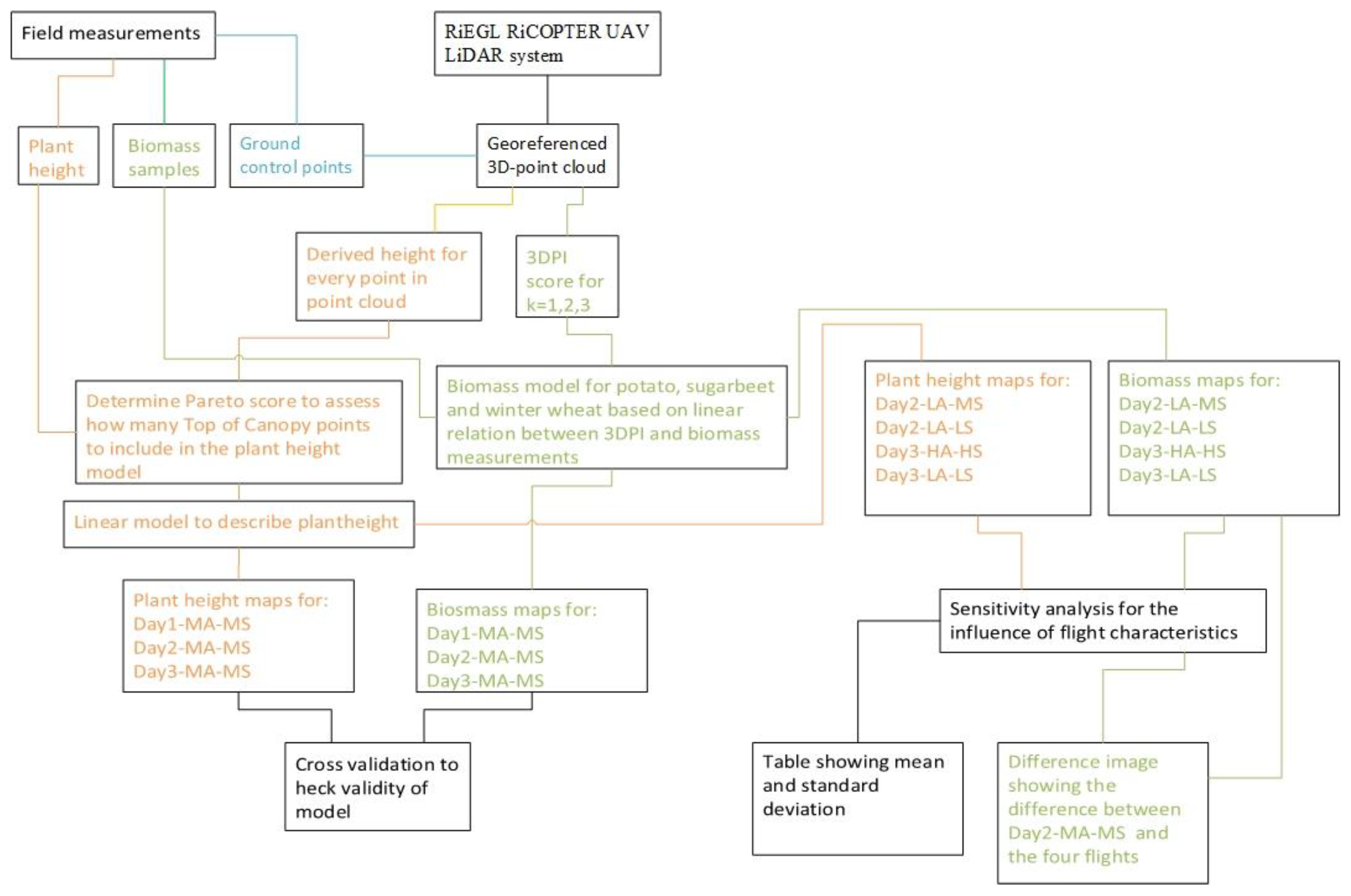
Overview of methodology for height and biomass retrieval from UAV-LiDAR observations for crops.
Figure 2.
Overview of methodology for height and biomass retrieval from UAV-LiDAR observations for crops.

Figure 3.
Scatter plots showing measured plant height vs derived plant height, where potato is based on the 10 highest points within a pixel, sugar beet on top 90 highest points, and winter wheat on the top 30 highest points. The blue line in the Figure is the 1:1 line.
Figure 3.
Scatter plots showing measured plant height vs derived plant height, where potato is based on the 10 highest points within a pixel, sugar beet on top 90 highest points, and winter wheat on the top 30 highest points. The blue line in the Figure is the 1:1 line.

Figure 4.
Error analysis for biomass derivation based on the 3-Dimensional Profile Index (3DPI) indicator, deviating K between 1, 2, or 3. Showing biomass estimations for potato, sugar beet, and winter wheat, including the dimensionless normalized in-sample.
Figure 4.
Error analysis for biomass derivation based on the 3-Dimensional Profile Index (3DPI) indicator, deviating K between 1, 2, or 3. Showing biomass estimations for potato, sugar beet, and winter wheat, including the dimensionless normalized in-sample.

Figure 5.
Scatter plots showing the relation between measured biomass and predicted for potato (k = 1), sugar beet (k = 3) and winter wheat (k = 1). The blue line in the Figure is the 1:1 line.
Figure 5.
Scatter plots showing the relation between measured biomass and predicted for potato (k = 1), sugar beet (k = 3) and winter wheat (k = 1). The blue line in the Figure is the 1:1 line.

Figure 6.
Scatterplot showing measured plant height versus LiDAR-derived plant height and the residual plot for the general plant height. Showing the model residuals versus fitted plant height. The colours in the left Figure show each separate crop. The blue line indicates the 1:1 line.
Figure 6.
Scatterplot showing measured plant height versus LiDAR-derived plant height and the residual plot for the general plant height. Showing the model residuals versus fitted plant height. The colours in the left Figure show each separate crop. The blue line indicates the 1:1 line.

Figure 7.
Scatter plot showing the relation between measured biomass and fitted biomass, for k = 3. The colours indicate the original crop data used for the model. The blue line in the Figure is the 1:1 line. On the right, the corresponding residual plot is shown. Showing the fitted plant height plotted against the model residuals.

Figure 8.
Profile plot for sugar beet showing a profile of 0.20 x 10 m. From top to bottom, it shows the flights DAY2-LA-MS, DAY2-LA-LS, DAY3-HA-HS, and DAY3-LA-LS. The green colours indicate plant material, where darker colours indicate a higher elevation of the point. The red points indicate the points classified as ground points.

Figure 9.
Maps indicating the estimated plant height in meters for sugar beet for DAY2-LA-MS, DAY2-LA-LS, DAY3-HA-HS, and DAY3-LA-LS. Darker greens indicate a higher plant height.
Figure 9.
Maps indicating the estimated plant height in meters for sugar beet for DAY2-LA-MS, DAY2-LA-LS, DAY3-HA-HS, and DAY3-LA-LS. Darker greens indicate a higher plant height.

Figure 10.
Maps indicating for flight DAY2-LA-MS, DAY2-LA-LS, DAY3-HA-HS, and DAY3-LA-LS the estimated biomass in grams for winter wheat. Darker greens mean a larger biomass prediction.
Figure 10.
Maps indicating for flight DAY2-LA-MS, DAY2-LA-LS, DAY3-HA-HS, and DAY3-LA-LS the estimated biomass in grams for winter wheat. Darker greens mean a larger biomass prediction.

Figure 11.
Maps indicating pixel differences between the biomass prediction for winter wheat of Flight Day2-MA-MS and, respectively, DAY2-LA-MS, DAY2-LA-LS, DAY3-HA-HS, and DAY3-LA-LS. Positive values (blue) indicate a higher prediction for, respectively, DAY2-LA-MS, DAY2-LA-LS, DAY3-HA-HS, and DAY3-LA-LS compared to Day2-MA-MS.


Table 1.
General information about the three crops planted in the study area.
| Crop Type | Sugar Beet | Potato | Winter Wheat |
|---|---|---|---|
| Fieldname | Dijkgraaf | Com02 | Braam |
| Planting month | April 2018 | April 2018 | October 2017 |
| Harvesting month | October 2018 | September 2018 | August 2018 |
| Size (hectare) | 1.99 | 2.0 | 1.78 |
Table 2.
Flying dates and corresponding growth stages for the crops in selected fields.
| Day | Date of Flight | Sugar Beet | Potato | Winter Wheat |
|---|---|---|---|---|
| 1 | 07-06-2018 | Vegetative | Vegetative/Tuber initiation | Heading |
| 2 | 25-06-2018 | Vegetative | Tuber bulking | Ripening |
| 3 | 27-06-2018 | Vegetative | Tuber bulking | Ripening |
| 4 | 11-07-2018 | Vegetative | Tuber bulking | Ripening |
Table 3.
Mean and standard deviation of field measurements separated per crop and sampling date.
| Crop | Sampling Date | Plant Height | Biomass Fresh Weight | ||||
|---|---|---|---|---|---|---|---|
| Sample Size | Mean (m) | Standard Deviation (m) | Sample Size | Mean (g/m2) | Standard Deviation (g/m2) | ||
| Potato | 07 June 2018 | 21 | 0.599 | 0.073 | 5 | 3364.93 | 461.65 |
| 25 June 2018 | 20 | 0.690 | 0.229 | 5 | 3546.40 | 846.19 | |
| 11 July 2018 | 20 | 0.547 | 0.151 | 5 | 3749.07 | 889.75 | |
| Sugar beet | 07 June 2018 | 16 | 0.275 | 0.098 | 5 | 1237.55 | 650.85 |
| 25 June 2018 | 20 | 0.501 | 0.099 | 5 | 3834.40 | 1374.40 | |
| 11 July 2018 | 15 | 0.445 | 0.105 | 5 | 3656.00 | 1191.38 | |
| Winter wheat | 07 June 2018 | 17 | 0.483 | 0.063 | 3 | 3477.37 | 751.71 |
| 25 June 2018 | 14 | 0.489 | 0.076 | 3 | 3371.67 | 940.45 | |
| 11 July 2018 | 20 | 0.449 | 0.076 | 3 | 1583.00 | 473.11 | |
Table 4.
Overview of flight dates, including flight codes and corresponding general flight details The flight codes are 1) indicating the flight number; 2) the flight altitude (LA = Low Altitude, MA = Medium Altitude, HA = High Altitude; 3) and flight speed (LS = Low Speed, MS = Medium Speed, HS = High Speed). Those codes will be used throughout the paper.
| Flight Date | Flight Number | Related Field Data | Code | Mean Flying Height (m.a.g.l.) | Mean Flying Speed (m/s) | Number of Flight Lines | Average Point Density (points/m2) | ||
|---|---|---|---|---|---|---|---|---|---|
| Wheat | Potato | Sugar Beet | |||||||
| 07-6-2018 | 1 | 07-6-2018 | Day1-MA-MS | 41.84 | 5.85 | 11 | 997 | 833 | 933 |
| 25-6-2018 | 1 | 25-6-2018 | Day2-MA-MS | 45.32 | 5.88 | 9 | 960 | 777 | 664 |
| 25-6-2018 | 2 | 25-6-2018 | Day2-LA-MS | 24.16 | 4.17 | 7 | 1516 | 659 | 805 |
| 25-6-2018 | 3 | 25-6-2018 | Day2-LA-LS | 20.05 | 2.73 | 5 | 2755 | 1402 | 1262 |
| 27-6-2018 | 1 | 25-6-2018 | Day3-HA-HS | 92.68 | 7.39 | 11 | 575 | 446 | 432 |
| 27-6-2018 | 2 | 25-6-2018 | Day3-LA-LS | 22.71 | 2.93 | 9 | 2257 | 2097 | 804 |
| 11-7-2018 | 1 | 11-7-2018 | Day4-MA-MS | 42.14 | 5.78 | 11 | 1011 | 873 | 1003 |
Table 5.
Overview of mean and standard deviation for the flights discussed in Figure 8, Figure 9 and Figure 10. The data for plant heights are from sugar beet, and the data for the biomass data are from the winter wheat maps. For Day1-MA-MS, Day2-MA-MS and Day4-MA-MS, there is no data (nd) in the difference cell because these were not compared to Day2-MA-MS.
| Flight | Plant Height (m) | Biomass (g/m2) | ||||||
|---|---|---|---|---|---|---|---|---|
| Data | Difference | Data | Difference | |||||
| Mean | SD | Mean | SD | Mean | SD | Mean | SD | |
| Day1-MA-MS | 0.186 | 0.096 | nd | nd | 2181.38 | 1182.68 | nd | nd |
| Day2-MA-MS | 0.443 | 0.153 | nd | nd | 2479.68 | 1133.56 | nd | nd |
| Day2-LA-MS | 0.445 | 0.149 | 0.002 | 0.050 | 2603.81 | 1164.33 | 96.80 | 1014.95 |
| Day2-LA-LS | 0.466 | 0.160 | 0.022 | 0.085 | 2720.69 | 1157.64 | 202.70 | 929.70 |
| Day3-HA-HS | 0.403 | 0.134 | 0.040 | 0.056 | 1622.14 | 1132.21 | –857.79 | 871.38 |
| Day3-LA-LS | 0.472 | 0.164 | 0.026 | 0.069 | 2435.03 | 1421.60 | –44.97 | 1018.49 |
| Day4-MA-MS | 0.445 | 0.136 | nd | nd | 2164.12 | 1261.95 | nd | nd |
© 2019 by the authors. Licensee MDPI, Basel, Switzerland. This article is an open access article distributed under the terms and conditions of the Creative Commons Attribution (CC BY) license (http://creativecommons.org/licenses/by/4.0/).
Share and Cite
MDPI and ACS Style
ten Harkel, J.; Bartholomeus, H.; Kooistra, L. Biomass and Crop Height Estimation of Different Crops Using UAV-Based Lidar. Remote Sens. 2020, 12, 17. https://0-doi-org.brum.beds.ac.uk/10.3390/rs12010017
AMA Style
ten Harkel J, Bartholomeus H, Kooistra L. Biomass and Crop Height Estimation of Different Crops Using UAV-Based Lidar. Remote Sensing. 2020; 12(1):17. https://0-doi-org.brum.beds.ac.uk/10.3390/rs12010017
Chicago/Turabian Styleten Harkel, Jelle, Harm Bartholomeus, and Lammert Kooistra. 2020. "Biomass and Crop Height Estimation of Different Crops Using UAV-Based Lidar" Remote Sensing 12, no. 1: 17. https://0-doi-org.brum.beds.ac.uk/10.3390/rs12010017
Note that from the first issue of 2016, this journal uses article numbers instead of page numbers. See further details here.