Understanding Tree-to-Tree Variations in Stone Pine (Pinus pinea L.) Cone Production Using Terrestrial Laser Scanner

Abstract

Kernels found in stone pinecones are of great economic value, often surpassing timber income for most forest owners. Visually evaluating cone production on standing trees is challenging since the cones are located in the sun-exposed part of the crown, and covered by two vegetative shoots. Very few studies were carried out in evaluating how new remote sensing technologies such as terrestrial laser scanners (TLS) can be used in assessing cone production, or in trying to explain the tree-to-tree variability within a given stand. Using data from 129 trees in 26 plots located in the Spanish Northern Plateau, the gain observed by using TLS data when compared to traditional inventory data in predicting the presence, the number, and the average weight of the cones in an individual tree was evaluated. The models using TLS-derived metrics consistently showed better fit statistics, when compared to models using traditional inventory data pertaining to site and tree levels. Crown dimensions such as projected crown area and crown volume, crown density, and crown asymmetry were the key TLS-derived drivers in understanding the variability in inter-tree cone production. These results underline the importance of crown characteristics in assessing cone production in stone pine. Moreover, as cone production (number of cones and average weight) is higher in crowns with lower density, the use of crown pruning, abandoned over 30 years ago, might be the key to increasing production in combination with stand density management.

1. Introduction

Three-dimensional arrangement of vegetation is of great importance in natural and in managed forest ecosystems. Canopy structure drives many functions such as light interception, habitat for fauna, and microenvironment regulation. Considering the inaccessibility and the complexity of large tree crown structures, it received little attention in the past. In the past decade, terrestrial laser scanning was increasingly used in many fields of forest science. These tools provide very accurate representation of the environment and allow unprecedented measurement of forest attributes at the stand and at the tree scale [1]. Traditional inventory metrics such as tree diameter and height can be extracted from TLS data, as well as precise positions of the trees within the stand [2,3]. A plethora of crown shape, crown volume, or crown deformation metrics can also be estimated [4,5], opening the way to accurately studying crown plasticity on large trees [6,7,8]. Moreover, material arrangement inside the crown and leaf area density (LAD) can also be quantified and used to estimate the amount of light intercepted and tree biomass production [8,9,10]. More recently, quantitative structural models (QSM) were linked to TLS data in order to reconstruct the trunk and branching system [11,12,13]. It is, thus, possible to study the whole tree topology and estimate wood volume and aboveground biomass of large trees [14,15]. TLS data are also largely used in an agricultural context as a phenotyping tool to estimate biomass production of crops [16]. Surprisingly, no study to our knowledge used TLS data to help modeling non-wood forest product in spite of its high potential to describe accurate tree metrics.

Cones of the Mediterranean stone pine (Pinus pinea L.) contain up to 120 edible seeds, called pine nuts, that constitute one of the most economically important non-wood forest products collected in the Mediterranean Basin. Spain, Portugal, Italy, and Turkey account for more than 90% of the total production of Mediterranean kernels in the world, attaining in an average year a total production over 4000 tons. The high price (60–70 €/kg) and low yield (3 to 4% kg kernel per kg cone) led forest owners to manage their forest to maximize cone production, such that owners obtain higher incomes from cone collection than from timber harvesting [17]. Assessing cone production is, thus, of high economical relevance for forest owners and managers.

The processes of flowering and fruiting in stone pine present a large spatiotemporal variability. It takes almost four years between the bud formation and seed dispersal after the natural dehiscence of cones. The female cone buds are set on the terminal shoots that are vigorous and dominant, mainly located on the outer part of the crown [18]. Masting (interannual and synchronized variability in cone production) is mainly controlled by the occurrence of rainfall events during the year prior to female floral emergence. However, the incidence of extreme freezing events, extended drought periods [19] or disturbances by native or exotic pests [20] can result in massive abortion of the conelets.

Large spatial variations in masting are found between regions, forests within a region, stands within a forest, and trees within a given stand [21]. Differences at larger scales are related to mean climatic conditions and soil water retention capacities. At a finer spatial resolution, large cone production is commonly found in mature stands where trees grow under lower levels of competition, permitting lateral expansion of the crowns. In these stands, dominant trees whose crowns are fully exposed to the sun and which define the upper-story layer of the forest have the highest yields. Thinning can increase cone production by increasing the available space for crown expansion of the residual trees [22]. The decrease in competition also improves tree vigor, which is associated with cone production [19,23]. Hence, crown volume was found to be a more important determinant of cone production than tree age or density [24].

Tree architecture of pine stone changes with its developmental stage. Young trees often have a spherical crown. As trees age, the crown shifts toward an umbrella shape, resulting from the polyarchic ramification, with the lateral branches of a whorl having higher diameter and length increments when compared to the branches of the main axis of the tree [25]. In addition, crown architecture shows a high phenotypic plasticity in response to light, favoring single shoots in shaded areas of the crowns while maximizing the number of codominant shoots in exposed branches [26]. The shape of the crown, the space available for crown expansion, and the number of exposed shoots, together with aspects such as the capacity of the forest soil to retain water or rainfall, all influence the number of cones a tree produces.

Visual assessment of cone production from the ground is highly challenging, since cones are located in the sun-exposed upper part of the crown and covered by two vegetative shoots. Estimation of the production is, thus, commonly carried out by means of predictive models (e.g., [19,21,27]). The observed temporal variability in cone production is accounted for either by including annual climate variables [19] or by considering as a response variable the observed average annual values for a set of years. Tree-to-tree variability is integrated into the model by using covariates such as diameter at breast height, distance-independent competition indices, and stand stocking metrics (e.g., stand basal area, absolute or relative stand density, site index). However, and despite the already mentioned importance of crown metrics and crown condition for the process of flowering and cone production, crown attributes are rarely considered, given the difficulty in measuring them. When used, crown diameter (measured as the vertical limit of the crown in one or two directions) or volume, estimated using crown diameter, depth, and shape, was found to explain some of the tree-to-tree variability (Rodrigues et al. 2014). These measures remain approximate, and detailed crown characteristics could help in furthering our understanding of why some trees in a stand produce more cones when compared to others. We believe that TLS technology can help in modeling crown production and understanding its functional drivers.

The objective of the present study is to better understand the relationship between tree characteristics and cone production in Mediterranean stone pine. This was achieved by quantifying the gain in using detailed crown metrics in estimating cone production at the individual tree level (number of cones per tree and average cone weight). Models based on traditional variables (tree size and stand characteristics) were compared to models that relied on crown metrics extracted from TLS data. The resulting models should help owners and managers to better predict cone production.

2. Materials and Methods

2.1. Study Region

The study sites were located on the Spanish Northern Plateau, a 50,000 km² plain area defined by the Duero river basin, with altitudes ranging from 600–900 m. This territory is characterized by a continental Mediterranean climate, with an average temperature of 12.6 °C, annual rainfall over 440 mm, and severe summer drought, resulting in an aridity index [28] of 0.60 (dry sub-humid). Soils have a high content of sand (>90%), with low content of nutrients and low water retention capacity. Only in the limestone areas (less than 15% of total area) do the soils have a higher clay content.

The forests within the region are pure pinewoods of Pinus pinea and Pinus pinaster, and mixtures of both species with Quercus ilex, Quercus faginea, and Juniperus thurifera. Pure Pinus pinea forests were retained, which represent more than 50% of the total forest area of the region, occupying more than 70,000 ha. Management of these forests is orientated to promote joint timber and cone production; thus, typical interventions consist of heavy and early thinnings to favor horizontal crown expansion, promotion of even-aged stands by application of shelterwood systems, and rotation lengths over 120 years.

2.2. Permanent Plots for Monitoring Cone Production

In 1996, a network of 141 permanent plots was installed in the study region. The main objective was to analyze the effect of forest management on timber and cone production (Figure 1). The complete ranges of site quality, stocking, and stand age were covered by the plots. The variable radius plots consisted of measuring the 20 closest trees to the plot center. At plot installation, diameter at breast height, total tree height, height to crown base, and crown diameter were measured on every tree, and tree coordinates were also recorded. The plots were remeasured on three occasions (2001, 2008 and 2016).

Cones were manually collected in all the plots every autumn from 1996 to 2005 by specialized climbers in the five trees closest to the center of the plot. The cones of each tree were counted and weighted. Since 2006, yearly cone collection is carried out on a subset of 30 plots. Only the cone production for 2016 and 2017 was used in the present work, as TLS acquisition was carried out in the fall of 2016. Furthermore, four of the 30 plots were not used as they were isolated from the other 26 plots, due to logistical constraints. Finally, a tree from one plot was dropped since the tree died after TLS data acquisition and cone collection, leading to 129 trees being used in the study (26 plots × 5 trees/plot—1 dead tree).

Table 1. Plot, tree and LiDAR level variables (with standard deviations in parenthesis).

Plot-Level Variables
Stand density (SD, st∙ha−1)	167 (101)
Stand age (A, years)	81.4 (27.3)
Basal area (BA, m2∙ha−1)	20.44 (10.02)
Mean quadratic diameter (MQD, cm)	40.3 (9.12)
Dominant stand height (domH, m)	12.56 (3.15)
Site index (SI, m)	15.33 (3.06)
Tree-level variables
Number of cones	14.1 (20.4)
Average cone weight (wt, g)	196.9 (74.2)
Diameter at breast height (dbh, cm)	40.9 (9.0)
Crown length (CL, m)	6.85 (1.44)
Crown diameter (CD, m)	7.30 (1.71)
Total tree height (H, m)	12.42 (3.16)
LiDAR-derived variables
Topographic position index (TPI)	0.0641 (0.0426)
Topographic roughness index (TRI)	0.0766 (0.0302)
Roughness (R)	0.1974 (0.0705)
Slope (S)	0.0778 (0.0451)
Crown length (CLL, m)	7.43 (1.91)
Projected crown area (PCA, m2)	54.65 (22.57)
Projected crown radius (CR, m)	4.09 (0.84)
Maximum crown radius (maxCr, m)	3.85 (0.82)
Crown surface area (SA, m2)	129.33 (64.36)
Crown volume (CV, m3)	189.27 (98.99)
Crown density (CDen)	0.4010 (0.1139)
Height to light crown base (LCB, m)	8.74 (3.47)
Light crown volume (LCV, m3)	104.66 (79.36)
Light crown surface area (LCSA, m2)	34.41 (33.68)
Light crown density (LCDen)	0.3656 (0.1107)
Crown asymmetry (ASYM)	0.5290 (0.1882)
Minimum projected crown radius (minCR, m)	2.89 (1.09)

presents the summary of plot, tree, and TLS-derived variables.

2.3. Terrestrial Laser Scanner Data Acquisition and Metric Extraction

The scanner used was a Faro Focus 3D. Each scan was performed with a resolution angle of 0.036° in both horizontal and vertical planes in combination with rotation angles of 360° horizontally and of 150° (from −60° to 90°) vertically. A multiscan approach consisting of merging several scans to increase three-dimensional (3D) representation accuracy was used. The individual scans were registered using 6–8 30 cm spherical targets distributed throughout the plot, and co-registration between scans was carried out with Faro Scene 6.2.2.7 (Faro Technologies Inc., Lake Mary, FL, USA). Finally, the stray point and dark filters were performed to remove noise points. Plots were scanned from five positions in October 2016, with the Faro Focus 3D placed for one scan in the center of the plot. The other four positions were chosen to minimize occlusion of the target trees and ensure that the crown of each sample tree was at least seen from three sides.

The co-registered point clouds were then exported to Computree (Othmani et al. 2011) to segment ground returns from tree points. The digital terrain model (DTM) was also obtained from CompuTree as a raster with 30 cm cells. The points from each sample tree were then manually isolated in R (R Development Core Team 2011) and CloudCompare (CloudCompare (GPL software) 2015). The DTM and isolated trees were then used to extract crown and micro-topographical metrics.

2.3.1. Crown Metrics

Crown base of the sample trees was estimated using a segmented regression with the segmented package in R [29,30]. Convex hulls were fitted on the XY-coordinates of sub point clouds every 10 cm along the Z-axis, and the maximum distance between the center and the vertices of the convex hull was recorded [31]. Crown base is defined as the lowest breakpoint of theses distances following the Z-axis, which corresponds to the point where the distance between the center and the vertices of the convex hull start to increase because of the presence of branches (Figure 2). The points above the crown base were then used to calculate the following previously published crown metrics [6]:

-

Crown volume (CV) and surface area (SA): volume and area of a 3D alpha-shape fitted to the points belonging to the crown cloud points;

-

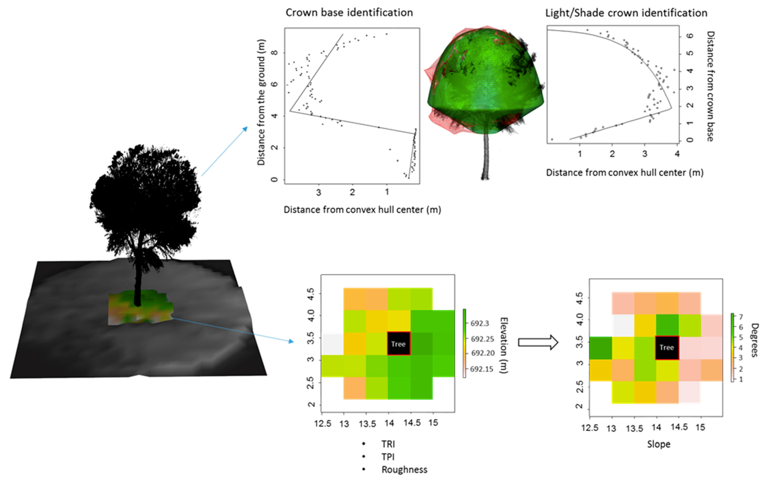
Light crown volume (LCV) and surface area (LCSA): the farthest distance from the crown center of each 10-cm slice of the crown was used to establish the maximum limits of the crown. A linear–log segmented regression was then used to find the transition between the shade and sun-exposed parts [32]. The volume and surface area of the crown above the transition zone were then calculated by fitting a 3D alpha-shape to the sun-exposed crown;

-

Height of the base of the sun-exposed crown (LCB): breakpoint of the linear–log segmented regression;

-

Crown length (CL): difference between total tree height and height to crown base;

-

Projected crown area (PCA): area of the projected crown on the XY-plane;

-

Maximum crown radius (maxCr): maximum of all the radii measured in each 10-cm slice of the crown;

-

Crown asymmetry (ASYM): ratio of the smallest and largest crown radius of the projected surface area;

-

Crown density: ratio of volume of non-empty 10 cm edged crown voxels to total crown volume, calculated for the complete crown (CDen) and the light crown only (LCDen).

2.3.2. Micro-Topography

The surrounding topography of each sample tree was quantified using the following metrics calculated with the 30-cm cell DTM raster (Figure 1):

-

Relative topographic position index (TPI): each surrounding cell of the tree is compared to the cell that contains the tree position by subtracting the height of the cell with the sample tree by mean height of the surrounding cells [33].

-

Relative ruggedness index (TRI): TRI is obtained by summing the difference in absolute values of the height of each neighboring cell and the height of the cell with the sample tree [34].

-

Roughness: difference between the maximum and minimum height of the cells surrounding the sample tree [35].

-

Slope: local slope calculated around the sample tree [36] using the slope method in the SDMTools package in R [37].

The micro-topographic metrics were calculated using 25 cell matrices (approximately 75-cm radius around the sample tree): the center cell of the matrix and the 24 neighboring cells of the DTM.

2.4. Data Analysis

The variables were divided into three groups: plot, tree, and TLS-derived metrics (Table 1). During preliminary analysis, high correlations were observed between several LiDAR-derived variables. In order to reduce the chances of observing (multi) collinearity during the modeling process, an initial principal component analysis (PCA) was carried out on the TLS-derived variables [38]. This was done to evaluate how correlated these were, and if variables were similar, to form groups of variables to be used in the modeling approach [39]. PCA was selected as it can easily detect patterns in a dataset by decomposing the variance–covariance matrix, and it is widely used to reduce the number of explanatory variables [39]. Furthermore, no a priori hypotheses were used to group the TLS-derived variables.

Models were then fitted for the following variable groups: (1) plot, (2) tree, (3) TLS, (4) plot and tree and (5) plot and TLS. For TLS variables, only one variable per group determined by the PCA results was included in a given model, i.e., if group 1 had variables W and X, and group 2 was composed of variables Y and Z, a model could have variable W, W, and Y or W and Z but not W and X. In the fifth case (plot and TLS), plot-level variables that could be obtained by TLS were kept (i.e., stand density (SD, st∙ha⁻¹), stand basal area (BA, m²∙ha⁻¹), mean quadratic diameter (MQD, cm), and dominant stand height (domH, m). For each analysis, all of the possible combinations of potential variables were tested, and the best model was the one with the lowest Akaike’s information criterion (AIC, for zero-inflated negative binomial regression) or Akaike’s information criterion corrected for small samples (AICc, for linear mixed model). Thus, a total of 63 models were compared for the plot-level variables (group 1), 15 for the tree level models (group 2), 449 for the TLS-derived variables (group 3), 1023 for the combined plot and tree levels (group 4), and 6735 for the combined plot and TLS levels (group 5).

2.4.1. Number of Cones

The number of cones (y_i) was modeled using a zero-inflated negative binomial regression (ZINB, Equation (1), [40]).

$$P\left(y_i=j\right)=\{\begin{array}{c}{\theta }_i+\left(1+{\theta }_i\right)g\left(y_i=0\right)\mathrm{if}j=0\\ \left(1-{\theta }_i\right)g\left(y_i\right)\mathrm{if}j>0\end{array}$$

(1)

where $g\left(y_i\right)$ is defined as

$$g\left(y_i\right)=P\left(Y=y_i|{\mu }_i,\alpha \right)=\frac{\mathsf{\Gamma }\left(y_i+{\alpha }^{-1}\right)}{\mathsf{\Gamma }\left(y_i\right)\mathsf{\Gamma }\left({\alpha }^{-1}\right)}{\left(\frac{1}{1+\alpha {\mu }_i}\right)}^{{\alpha }^{-1}}{\left(\frac{\alpha {\mu }_i}{1+\alpha {\mu }_i}\right)}^{y_i}$$

(2)

The mean ${\mu }_i$ is then related to the covariates as follows:

$${\mu }_i=\exp \left(\mathbf{X}\beta +{\mu }_i\right)$$

(3)

where X and 𝛽 are the covariate matrix and estimated fixed effect vector, respectively. ${\theta }_i$ is given by the logistic function

$${\theta }_i=1-\frac{{\lambda }_i}{1+{\lambda }_i}$$

(4)

where

$${\lambda }_i=\exp \left(\mathbf{Z}\gamma +v_i\right)$$

(5)

where Z and γ are the covariate matrix and estimated fixed effect vector, respectively.

Finally, plot-level random effects were included as ${\mu }_i$ and $v_i$, where ${\mu }_i~N\left(0,{\sigma }_{1i}^2\right)$ and $v_i~N\left(0,{\sigma }_{2i}^2\right)$. The model was calibrated using the GLMMadaptive library in R [41].

Variable selection was carried out for the negative binomial (Equation (3)) and logistic regression (Equation (4)) separately for each of the variable groups. These were calibrated using the lme4 library in R [42]. Model comparison was carried out using the AICcmodavg package in R [43]. The logistic and negative binomial parts were then combined in the ZINB model, and variables with a significance level larger than 0.10 (i.e., p > 0.10) were discarded. Some variables were standardized in order to allow for convergence. The standardized variables are indicated with an asterisk, i.e., TPI* is the standardized value of TPI.

2.4.2. Average Cone Weight

Average cone weight (w_ij) was predicted using a linear mixed effect model including a plot and year crossed random effect (Equation (6)).

$$w_{ijk}=\mathbf{T}\delta +s_i+t_i+{ϵ}_{ijk}$$

(6)

where T and δ are the covariable matrix and fixed effect parameter vector, respectively. $s_i$, $t_i$ and ${ϵ}_{ijk}$ are the plot and year random effects and residual error, where $s_i~N\left(0,{\sigma }_{3i}^2\right)$, $t_i~N\left(0,{\sigma }_{4i}^2\right)$ and ${ϵ}_{ijk}~N\left(0,{\sigma }_{ijk}^2\right)$. These models were also calibrated using the lme4 package in R.

3. Results

The PCA analysis indicated that the TLS-derived variables could be grouped into four categories (Figure 3). The first group contained variables quantifying the local topography around a tree: TPI, TRI, slope, and roughness. The second was composed of variables that measure crown dimensions: crown volume and surface area, light crown volume and surface area, average crown and average crown projected area radius, maximum crown radius, height to light crown base, and crown length. The third was related to crown asymmetry: crown asymmetry and smallest projected crown radius. Finally, the fourth group estimated the density of the crown: total crown density and light crown density. The mean intra- and inter-group Euclidian distances indicated that variables from a given group were closer than the groups (

Table 2. Euclidean distances between variables in a same group (average, diagonal) and between groups (group centers obtained by geometric mean of each variable in a group, lower triangle).

	Topography	Crown Dimensions	Crown Density	Crown Asymmetry
Topography	0.57
Crown dimensions	1.04	0.22
Crown density	1.24	1.57	0.17
Crown asymmetry	1.22	0.92	1.17	0.45

). In the analysis using TLS metrics, only one of the variables of a given group could be found in a given model. In other words, if TPI was included in a model, the other topographic variables (i.e., TRI, slope, or roughness) were not included.

Based only on plot-level variables, the average number of cones a tree has was conditioned by the mean quadratic diameter, stand density, site index, and stand basal area (Equations (7) and (8)).

$${\lambda }_i=\exp \left(4.8403-0.1698 \mathrm{MQD}\right)$$

(7)

$${\mu }_i=\exp \left(0.4393+0.1143 \mathrm{SI}+0.0521 \mathrm{BA}-0.0087 \mathrm{SD}\right)$$

(8)

The probability of observing a tree with cones increased with the mean quadratic diameter (−0.1698, p = 0.0647). The number of cones, when present, increased with both site index (0.1143, p = 0.0781) and basal area (0.0521, p = 0.0274) and decreased with stand density (−0.0087, p = 0.0008).

When uniquely considering the tree-level variables, the best model indicated that the presence of cones increased with crown diameter (−1.0944, p = 0.0008, Equation (9)), and the number of cones increased with both tree diameter (0.0432, p = 0.0054, Equation (10)) and crown length (0.2307, p = 0.0024).

$${\lambda }_i=\exp \left(5.5133-1.0944 \mathrm{CD}\right)$$

(9)

$${\mu }_i=\exp \left(-1.4369+0.0432 \mathrm{DBH}+0.2307 \mathrm{CL}\right)$$

(10)

When plot- and tree-level variables were combined, plot-level variables were included only in the negative binomial (abundance) part of the model (Equations (11) and (12)).

$${\lambda }_i=\exp \left(5.9127-1.1581 \mathrm{CD}\right)$$

(11)

$${\mu }_i=\exp \left(-1.0342+0.0299 \mathrm{DBH}+02392 \mathrm{CL}-1.2539 {\mathrm{SD}}^{*}+0.8163 {\mathrm{BA}}^{*}-0.6435 {\mathrm{MQD}}^{*}\right)$$

(12)

The same trends as those found in the plot- and tree-level models were also observed; the probability of presence of cones increased with crown diameter (−1.1581, p = 0.0002), while the number of cones increased with tree diameter (0.0299, p = 0.0812), crown length (0.2392, p = 0.0011), and stand basal area (scaled, 0.8163, p = 0.0095) and decreased with stand density (scaled, −1.2539, p = 0.0024) and stand mean quadratic diameter (scaled, −0,6435, p = 0.0719).

When TLS-derived metrics were used to predict the number of cones, crown dimension and asymmetry variables entered the model for the presence of cones, and crown dimension and crown density group variables influenced the number of cones (Equations (13) and (14)).

$${\lambda }_i=\exp \left(7.8285-2.0151 \mathrm{PCA}-0.9438 \mathrm{minCR}\right)$$

(13)

$${\mu }_i=\exp \left(2.7672+0.5019 {\mathrm{CV}}^{*}-2.3075 \mathrm{CDen}\right)$$

(14)

The probability of observing cones increased with the projected crown area (−2.0151, p = 0.0089) and the minimum crown radius (−0.9438, p = 0.0152). When the cones were present, their number increased with crown volume (scaled, 0.5019, p < 0.0001) and decreased with crown density (−2.3075, p = 0.0630).

The covariates included in the logistic part (occurrence) of the zero-inflated negative binomial regression did not change when plot-level variables were evaluated together with TLS-derived metrics (Equation (15)), where the probability of observing cones increased again with the crown projected area (−1.7677, p = 0.0094) and minimum crown radius (−0.9318, p = 0.0126). The number of cones, when present, also varied with crown volume (scaled, 0.4890, p < 0.0001, Equation (16)). When compared to Equation (14), crown density was replaced by stand density (scaled, −0.6056, p = 0.0058), mean quadratic diameter (−0.8399, p = 0.0362) and dominant stand height (0.3532, p = 0.0023).

$${\lambda }_i=\exp \left(7.0639-1.7677 \mathrm{PCA}-0.9318 \mathrm{minCR}\right)$$

(15)

$${\mu }_i=\exp \left(-2.7613+0.4890 {\mathrm{CV}}^{*}-0.6056 {\mathrm{SD}}^{*}-0.8399 {\mathrm{MQD}}^{*}+0.3532 \mathrm{domH}\right)$$

(16)

The models with TLS-derived variables performed the best, based on AIC (

Table 3. Akaike’s information criterion (AIC) and variance estimates for the zero-inflated negative binomial regressions (Equations (3) and (5)).

Model	Number of Variables in Logistic Component	Number of Variables in Negative Binomial Component	${\mathit{\sigma }}_{1\mathit{i}}^2$	${\mathit{\sigma }}_{2\mathit{i}}^2$	Log (Dispersion)	AIC	AIC Weight
0. Null model	0	0	1.0280	2.9193	0.2140	1400.19	>0.0001
1. Plot	1	3	0.4256	4.6833	0.2266	1383.76	>0.0001
2. Tree	1	2	0.5222	3.3970	0.4205	1349.8	0.0001
3. LST	2	2	0.4850	5.5951	0.4788	1337.01	0.0816
4. Plot and tree	1	5	0.3926	3.2902	0.4324	1346.53	0.0007
5. Plot and LST	2	4	0.4252	4.6492	0.5127	1332.17	0.9176

). Of the two models with TLS covariates, the plot and TLS model had the lowest AIC. The AIC weights for both models containing TLS-derived variables summed to 0.999 (Table 3). These weights can be interpreted as the summed conditional probability for both models [44]. The next models were the ones with tree-level variables, with the best one having both plot- and tree-level variables. The model showing the worst fit was the one with only plot-level information.

The average weight of the cones was proportional to the site index when only plot-level variables were used (6.646, p = 0.0292, Equation (17)). The average weight was found to be proportional to tree height in the case of the models with tree-level variables (5.359, p = 0.0473, Equation (18)). When both plot- and tree-level variables were used, the model with the lowest AIC was the same as the tree-level model (Equation (18)). The average weight was proportional to the surface area of the light crown (0.2543, p = 0.0423, Equation (19)) and inversely proportional to the light crown density (−103.3775, p = 0.0433) when TLS-derived variables were considered. Finally, roughness (88.1099, p = 0.1497, Equation (20)) and stand density (−0.0940, p = 0.3214) were also included with the light crown surface area (0.2517, p = 0.0447) and light crown density (−88.5663, p = 0.0853) in the plot and TLS model.

$$w_{ijk}=28.804+6.646 \mathrm{SI}$$

(17)

$$w_{ijk}=65.784+5.359 \mathrm{H}$$

(18)

$$w_{ijk}=160.0430+0.2543 \mathrm{LCSA}-103.7775 \mathrm{LCDen}$$

(19)

$$w_{ijk}=151.9019+0.2517 \mathrm{LCSA}-88.5663 \mathrm{LCDen}+88.1099 \mathrm{R}-0.0940 \mathrm{SD}$$

(20)

As with the zero-inflated negative binomial models, the average cone weight models that included TLS-derived variables had the lowest AIC (

Table 4. Akaike’s information criterion (AIC) and variance estimates for the mean cone average weight (Equation (6)).

Model	Number of Variables	${\mathit{\sigma }}_{3\mathit{i}}^2$	${\mathit{\sigma }}_{4\mathit{i}}^2$	${\mathit{\sigma }}_{\mathit{i}\mathit{j}\mathit{k}}^2$	AICc	AIC Weight
0. Null	0	1788	8190	2132	1814.91	0.0002
1. Plot	1	1418	8195	2131	1807.89	0.0072
2. Tree	1	1754	8377	2092	1809.12	0.0039
3. LiDAR	2	1418	8295	2105	1803.78	0.0562
4. Plot and tree	1	1754	8377	2092	1809.12	0.0039
5. Plot and liDAR	4	1257	8306	2123	1798.17	0.9286

), with the plot and TLS model having the lowest AICc. Moreover, the AICc weights supported the models with TLS-derived variables, with both models containing TLS variables accounting for 0.98 of the weight (Table 4). The models with plot- and/or tree-level variables had AICc values that were very close, with a spread of 1.23 points between the best and worst. These models, thus, could not be very well discriminated (Burnham and Anderson, 2002).

4. Discussion

Inter-site and inter-annual stone pinecone production, defined as either cone presence, number of cones in a tree, or average cone weight, is fairly well understood. Tree size [21,45], competition [46,47] (Freire, 2009, Piqué et al., 2015), stand stocking [27,48], stand maturity, and site conditions [49] all influence the presence and number of cones found in a tree. Certain crown dimensions, such as crown length, which positively enters the model for cone production, can be considered a good indicator of inter-tree competition for light. However, the differences in production between two trees in the same stand, of similar status and dimensions, are not well understood. It was, thus, intended to use more detailed crown and microsite information obtained by TLS to better understand the between-tree variations.

In order to quantify the improvements by the addition of TLS variables in understanding tree-to-tree variability, models using inventory-based plot- and tree-level variables were compared to one using TLS-derived metrics and one using all potential variables (inventory and TLS). The probability of a tree bearing cones and the total number of cones were positively related with tree and crown size and negatively with stand density. Basal area, which reduces cone production, was statistically significant when stand density was also present, and it can be considered as a proxy of both stand maturity and site index. As for average cone weight, it was found to increase with tree height and site index. These results, pointing to higher cone production in older trees with larger crowns growing under low stocking levels, were already reported for stone pine [19,50], as well as for other species [51,52,53].

Water availability in the soil is important for female flower emergence, cone survival, and enlargement [26]. Water availability is intrinsically related to topography. At larger scales, inter-site water availability is explained by total rainfall and soil texture. Irregularity of the terrain influences the intra-site water availability. This was captured by the roughness index obtained from the digital terrain model surrounding the tree. Higher roughness indices indicated more irregular terrain, which could be due to depressions and microbasins. This would, thus, indicate that trees found on such microtopographical locations have access to more water, leading to cones with more biomass.

Very few studies looked at the links between crown dimensions and cone production. Rodrigues et al. [27] found that trees with larger crowns have more cone biomass. Crown width or length, measured during field surveys as measured by Rodrigues et al. [27], are imprecise when compared to metrics that can be obtained from remote sensing such as TLS. Of all the tested TLS covariates, crown projected area and minimum crown radius replaced inventory-based crown diameter when trying to segregate trees with and without cones in the present study. While crown diameter and crown projected area both measure the same dimensions (larger crowns have more probability of bearing cones), trees with a smaller minimum crown radius for a given projected area have an asymmetric crown. Asymmetric crowns are largely associated with lateral inter-tree competition which prevents crown expansion on all sides, reducing the probability of observing cones in the tree. It is interesting to point out that adjacent trees on unmanaged forests can have intermingled crowns such that they ultimately share a single umbrella shaped crown in order to maximize light acquisition [18]. Such fused crowns were, however, not observed in the dataset, since our study area was mainly composed of forests intensively managed to promote cone production, where early and heavy thinning is applied aiming at maximum lateral crown expansion but preventing crown interlacing.

The number of cones in a stone pine tree is determined by both the volume and the density of the crown. TLS-derived crown volume captures irregularities and asymmetries in the crown shape, going beyond the common simplification of circular-shape projected area and regular ellipsoid approximation of crown volume. In both cases (either from ground-estimated or TLS-measured crown volume), trees with larger crowns have more cones, as the number of shoots that can bear cones increases with crown size. The decrease in the number of cones with crown density could be explained by two hypotheses. Firstly, stone pine crown architecture varies with tree ontogeny. The spherical crown with foliage covering the whole external surface of young trees shifts toward a smoothly rounded umbrella-like shape with foliage only covering the upper, fully sun-exposed part of the crown, while the lower part of the crown has very little foliage [25,26,54]. As the measured crown density decreases with tree age, crown density may act as a proxy of tree maturity. Moreover, since mature trees produce more cones, a decrease in their number with increasing crown density is expected. On the other hand, a more physiological-based explanation can also be detailed. In denser crowns, the tree has to allocate resources (e.g., water, photosynthates, nutrients) to less vigorous and shaded branches in the inner and lower part of the crown, which commonly does not bear female conelets [18,26]. There are, thus, fewer resources left for reproductive organs, and the number of cones, thus, decreases.

The average weight of the cones is also inversely proportional to the density of the sun-exposed part of the crown. This result reflects the importance of light for reproductive shoots and branches bearing cones, where the resources assimilated are directly allocated to the enlargement of the cones. The same physiological argument can be put forward, whereby resources in denser crowns have to be allocated to the maintenance of non-reproductive shoots. Conversely, self-shading and light occlusion over the maturing cones, as they are located below two vegetative shoots, can result in losses in the photosynthetic activity of the cones in very dense crowns [55]. This would result in a reduction on the available photosynthates for cone development and enlargement.

These results shed light on the relevance of crown architecture on the whole process of female flowering and further cone enlargement in the species. The importance of crown dimensions and density has practical implications if cone production is to be maximized. Crown pruning (or poda de olivación in Spanish) consists of clipping the non-vigorous and dead branches of the inner part of the crown, in order to promote the emergence of female flowers in the following spring [50]. While widely practiced in Spain up to 30 years ago, this treatment is currently abandoned since no scientific evidence of significant increment in cone production justifies the high cost of the practice. Our results are in agreement with recent experiences [56] giving support to the idea of enhanced floral emergence in less dense crowns. The relationship between crown density, flowering, and cone maturation is nevertheless needed to establish the increase in cone production after pruning, after which the economic viability can be assessed.

Most of the TLS-derived metrics that are included in the models cannot easily be measured through traditional inventories. For example, crown projected area and minimum crown dimensions can be measured from the ground (presence/absence of cones). However, light and total crown volume/density (number of cones and average cone weight) cannot be estimated by survey crews. These variables improve model fit statistics and help better understand the important drivers that are not yet considered in understanding cone production.

5. Conclusions

When compared, the models based on TLS metrics clearly outperformed the inventory-based models, indicating that crown dimensions are an important driver in understanding cone production in stone pine. In this sense, our work points to the potential of using TLS as a tool for rapid, accurate, and unbiased measurements of crown parameters not easily accessible from the ground. Moreover, the links between crown dimensions and cone production should be further investigated to better understand the physiological processes involved, in order to both propose management practices to maximize production and better integrate the processes in prediction models. Nevertheless, managers should favor growing conditions that enable the trees to develop large, symmetrical crowns. Crown pruning should also be considered to increase cone production. Finally, the TLS attributes that were found to be important (e.g., crown volume, density, terrain roughness) can also be derived from other remote sensing sensors such as aerial or drone LiDAR. Quick, large-area estimates of cone production could ultimately be achieved and help managers identify areas of high cone productivity. Thus, such sensors might reduce the costs in estimating cone production.

References

1. Dassot, M.; Colin, A.; Santenoise, P.; Fournier, M.; Constant, T. Terrestrial laser scanning for measuring the solid wood volume, including branches, of adult standing trees in the forest environment. Comput. Electron. Agric. 2012, 89, 86–93. [Google Scholar] [CrossRef]
2. Liang, X.; Kankare, V.; Hyyppä, J.; Wang, Y.; Kukko, A.; Haggrén, H.; Yu, X.; Kaartinen, H.; Jaakkola, A.; Guan, F. Terrestrial laser scanning in forest inventories. ISPRS J. Photogramm. Remote Sens. 2016, 115, 63–77. [Google Scholar] [CrossRef]
3. Maas, H.-G.; Bienert, A.; Scheller, S.; Keane, E. Automatic forest inventory parameter determination from terrestrial laser scanner data. Int. J. Remote Sens. 2008, 29, 1579–1593. [Google Scholar] [CrossRef]
4. Barbeito, I.; Dassot, M.; Bayer, D.; Collet, C.; Drössler, L.; Löf, M.; Del Rio, M.; Ruiz-Peinado, R.; Forrester, D.I.; Bravo-Oviedo, A. Terrestrial laser scanning reveals differences in crown structure of Fagus sylvatica in mixed vs. pure European forests. For. Ecol. Manag. 2017, 405, 381–390. [Google Scholar] [CrossRef]
5. Seidel, D.; Leuschner, C.; Müller, A.; Krause, B. Crown plasticity in mixed forests—Quantifying asymmetry as a measure of competition using terrestrial laser scanning. For. Ecol. Manag. 2011, 261, 2123–2132. [Google Scholar] [CrossRef]
6. Martin-Ducup, O.; Schneider, R.; Fournier, R.A. Response of sugar maple (Acer saccharum, Marsh.) tree crown structure to competition in pure versus mixed stands. For. Ecol. Manag. 2016, 374, 20–32. [Google Scholar]
7. Metz, J.; Seidel, D.; Schall, P.; Scheffer, D.; Schulze, E.-D.; Ammer, C. Crown modeling by terrestrial laser scanning as an approach to assess the effect of aboveground intra- and interspecific competition on tree growth. For. Ecol. Manag. 2013, 310, 275–288. [Google Scholar] [CrossRef]
8. Pimont, F.; Allard, D.; Soma, M.; Dupuy, J.-L. Estimators and confidence intervals for plant area density at voxel scale with T-LiDAR. Remote Sens. Environ. 2018, 215, 343–370. [Google Scholar] [CrossRef]
9. Béland, M.; Widlowski, J.L.; Fournier, R.A.; Côté, J.F.; Verstraete, M.M. Estimating leaf area distribution in savanna trees from terrestrial LiDAR measurements. Agric. For. Meteorol. 2011, 151, 1252–1266. [Google Scholar] [CrossRef]
10. Martin-Ducup, O.; Schneider, R.; Fournier, R. Analyzing the Vertical Distribution of Crown Material in Mixed Stand Composed of Two Temperate Tree Species. Forests 2018, 9, 673. [Google Scholar] [CrossRef] [Green Version]
11. Côté, J.-F.; Fournier, R.A.; Frazer, G.W.; Niemann, K.O. A fine-scale architectural model of trees to enhance LiDAR-derived measurements of forest canopy structure. Agric. For. Meteorol. 2012, 166, 72–85. [Google Scholar] [CrossRef]
12. Hackenberg, J.; Spiecker, H.; Calders, K.; Disney, M.; Raumonen, P. SimpleTree—an efficient open source tool to build tree models from TLS clouds. Forests 2015, 6, 4245–4294. [Google Scholar] [CrossRef]
13. Raumonen, P.; Kaasalainen, M.; Åkerblom, M.; Kaasalainen, S.; Kaartinen, H.; Vastaranta, M.; Holopainen, M.; Disney, M.; Lewis, P. Fast Automatic Precision Tree Models from Terrestrial Laser Scanner Data. Remote Sens. 2013, 5, 491–520. [Google Scholar] [CrossRef] [Green Version]
14. Gonzalez de Tanago, J.; Lau, A.; Bartholomeus, H.; Herold, M.; Avitabile, V.; Raumonen, P.; Martius, C.; Goodman, R.C.; Disney, M.; Manuri, S. Estimation of above-ground biomass of large tropical trees with terrestrial LiDAR. Methods Ecol. Evol. 2018, 9, 223–234. [Google Scholar] [CrossRef] [Green Version]
15. Momo Takoudjou, S.; Ploton, P.; Sonké, B.; Hackenberg, J.; Griffon, S.; De Coligny, F.; Kamdem, N.G.; Libalah, M.; Mofack, G.I.; Le Moguédec, G. Using terrestrial laser scanning data to estimate large tropical trees biomass and calibrate allometric models: A comparison with traditional destructive approach. Methods Ecol. Evol. 2018, 9, 905–916. [Google Scholar] [CrossRef]
16. Guo, Q.; Wu, F.; Pang, S.; Zhao, X.; Chen, L.; Liu, J.; Xue, B.; Xu, G.; Li, L.; Jing, H. Crop 3D—a LiDAR based platform for 3D high-throughput crop phenotyping. Sci. China Life Sci. 2018, 61, 328–339. [Google Scholar] [CrossRef]
17. Ovando, P.; Campos, P.; Calama, R.; Montero, G. Landowner net benefit from stone pine (Pinus pinea L.) afforestation of dry-land cereal fields in Valladolid, Spain. J. For. Econ. 2010, 16, 83–100. [Google Scholar] [CrossRef]
18. Mutke, S.; Sievänen, R.; Nikinmaa, E.; Perttunen, J.; Gil, L. Crown architecture of grafted Stone pine (Pinus pinea L.): shoot growth and bud differentiation. Trees 2005, 19, 15–25. [Google Scholar] [CrossRef]
19. Calama, R.; Alonso, F.J.G.; Casanueva, G.M.; Regneri, S.M.; Conde, M.; González, G.M.; Minguez, M.P. Enhanced tools for predicting annual stone pine (Pinus pinea L.) cone production at tree and forest scale in inner Spain. For. Syst. 2016, 25, 14. [Google Scholar] [CrossRef] [Green Version]
20. Mutke, S.; Calama, R.; Nasrallah Neaymeh, E.; Roques, A. Impact of the Dry Cone Syndrome on commercial kernel yield of stone pine cones. In Options Méditerranéennes Sér. Sémin. Méditerranéens; CIHEAM: Zaragoza, Spain, 2017; pp. 79–84. [Google Scholar]
21. Calama, R.; Gordo, F.J.; Mutke, S.; Montero, G. An empirical ecological-type model for predicting stone pine (Pinus pinea L.) cone production in the Northern Plateau (Spain). For. Ecol. Manag. 2008, 255, 660–673. [Google Scholar] [CrossRef]
22. Moreno-Fernández, D.; Cañellas, I.; Calama, R.; Gordo, J.; Sánchez-González, M. Thinning increases cone production of stone pine (Pinus pinea L.) stands in the Northern Plateau (Spain). Ann. For. Sci. 2013, 70, 761–768. [Google Scholar] [CrossRef] [Green Version]
23. Loewe, V.; Venegas, A.; Delard, C.; González, M. Thinning effect in two young stone pine plantations (Pinus pinea L.) in central southern Chile. Opt. Méditerranéennes 2013, 105, 44–55. [Google Scholar]
24. Boutheina, A.; El-Aouni, M.H.; Balandier, P. Influence of stand and tree attributes and silviculture on cone and seed productions in forests of Pinus pinea L. in northern Tunisia. Opt. Méditerranéennes Sér. Sémin. Méditerranéens 2013, 105, 9–14. [Google Scholar]
25. Ruiz de la Torre, J. Árboles y arbustos de la España peninsular. ETS Ing. Montes Madr. Spain 1979. [Google Scholar]
26. Mutke, S.; Calama, R.; González-Martínez, S.C.; Montero, G.; Javier Gordo, F.; Bono, D.; Gil, L. Mediterranean Stone Pine: Botany and Horticulture. Hortic. Rev. 2012, 39, 153–201. [Google Scholar]
27. Rodrigues, A.; Silva, G.L.; Casquilho, M.; Freire, J.; Carrasquinho, I.; Tomé, M. Linear mixed modelling of cone production for Stone Pine in Portugal. Silva Lusit. 2014, 22, 1–27. [Google Scholar]
28. United Nations Environment Programme (UNEP) World atlas of desertification. In World Atlas of Desertification; UNEP: Nairobi, Kenya, 1992.
29. Muggeo, V.M.R. Estimating regression models with unknown break-points. Stat. Med. 2003, 22, 3055–3071. [Google Scholar] [CrossRef]
30. Muggeo, V.M. Segmented: an R package to fit regression models with broken-line relationships. R News 2008, 8, 20–25. [Google Scholar]
31. Barber, C.B.; Habel, K.; Grasman, R.; Stahel, A.; Stahel, A.; Sterratt, D.C. Geometry: Mesh Generation and Surface Tesselation. 2014. Available online: https://davidcsterratt.github.io/geometry/ (accessed on 2 January 2020).
32. Pretzsch, H. Forest Dynamics, Growth and Yield: From Measurement to Model; Springer: Berlin, Germany, 2009. [Google Scholar]
33. Riley, S.J. Index that quantifies topographic heterogeneity. Intermt. J. Sci. 1999, 5, 23–27. [Google Scholar]
34. Wilson, M.F.; O’Connell, B.; Brown, C.; Guinan, J.C.; Grehan, A.J. Multiscale terrain analysis of multibeam bathymetry data for habitat mapping on the continental slope. Mar. Geod. 2007, 30, 3–35. [Google Scholar] [CrossRef] [Green Version]
35. Dartnell, P. Applying Remote Sensing Techniques to Map Seafloor Geology/Habitat Relationships. Ph.D. Thesis, San Francisco State University, San Francisco, CA, USA, 2000. [Google Scholar]
36. Burrough, P.A.; McDonnell, R.; McDonnell, R.A.; Lloyd, C.D. Principles of Geographical Information Systems; Oxford University Press: Oxford, UK, 2015. [Google Scholar]
37. VanDerWal, J.; Falconi, L.; Januchowski, S.; Shoo, L.; Storlie, C. SDMTools: Species Distribution Modelling Tools: Tools for processing data associated with species distribution modelling exercises. R Package Version 2014, 1, 1–221. [Google Scholar]
38. King, J.R.; Jackson, D.A. Variable selection in large environmental data sets using principal components analysis. Environmetrics 1999, 10, 67–77. [Google Scholar] [CrossRef]
39. Quinn, G.G.P.; Keough, M.J. Experimental Design and Data Analysis for Biologists; Cambridge University Press: Cambridge, UK, 2002. [Google Scholar]
40. Hall, D.B. Zero-Inflated Poisson and Binomial Regression with Random Effects: A Case Study. Biometrics 2000, 56, 1030–1039. [Google Scholar] [CrossRef] [PubMed]
41. Rizopoulos, D. GLMMadaptive: Generalized Linear Mixed Models Using Adaptive Gaussian Quadrature. R Package Version 0.4-0. 2018. Available online: https://rdrr.io/cran/GLMMadaptive/man/GLMMadaptive.html (accessed on 27 December 2019).
42. Bates, D.; Bolker, B.; Walker, S. Fitting linear mixed-effects models using lme4. J. Stat. Softw. 2015, 67, 1–48. [Google Scholar] [CrossRef]
43. Mazerolle, M.J. AICcmodavg: Model Selection and Multimodel Inference Based on (Q)AIC(c); Universidade de Lisboa: Lisbon, Portugal, 2017. [Google Scholar]
44. Wagenmakers, E.-J.; Farrell, S. AIC model selection using Akaike weights. Psychon. Bull. Rev. 2004, 11, 192–196. [Google Scholar] [CrossRef] [PubMed]
45. Cañadas, M.N. Pinus pinea L. en el Sistema Central (Valles del Tiétar y del Alberche): desarrollo de un modelo de crecimiento y producción de piña. Ph.D. Thesis, Universidad Politécnica de Madrid, Madrid, Spain, 2000. [Google Scholar]
46. Freire, J.P.A. Modelação do crescimento e da produção de pinha no pinheiro manso. Ph.D. Thesis, ISA-UTL Lisbon Port, Lisboa, Portugal, 2009. [Google Scholar]
47. Piqué, M.; Vericat, P.; Beltran, M.; Calama, R.; Cervera, T. Models de Gestió per a les Pinedes de pi Pinyer (Pinus pinea L.): Producció de Fusta i Pinya i Prevenció de Incendis Forestales; Centre de la Propietat Forestal. Departament d’Agricultura, Ramaderia, Pesca, Alimentació i Medi Natural; Generalitat de Catalunya: Barcelona, Spain, 2016; ISBN B17190-2015. [Google Scholar]
48. Castellani, C. La produzione legnosa e del fruto e la durata economico delle pinete coetanee di pino domestico (Pinus pinea L.) in un complesso assestato a prevalente funzione produttiva in Italia. Ann. ISAFA 1989, 12, 161–221. [Google Scholar]
49. Calama, R.; Mutke, S.; Tomé, J.; Gordo, J.; Montero, G.; Tomé, M. Modelling spatial and temporal variability in a zero-inflated variable: The case of stone pine (Pinus pinea L.) cone production. Ecol. Model. 2011, 222, 606–618. [Google Scholar] [CrossRef]
50. Montero, G.; Calama, R.; Ruiz Peinado, R. Selvicultura de Pinus pinea L. In Compendio de Selvicultura de Especies. INIA: Fundación Conde del Valle de Salazar, Madrid; INIA Andes: Montevideo, Uruguay, 2008; pp. 431–470. [Google Scholar]
51. Sirois, L. Spatiotemporal variation in black spruce cone and seed crops along a boreal forest-tree line transect. Can. J. For. Res. 2000, 30, 900–909. [Google Scholar] [CrossRef]
52. Verkaik, I.; Espelta, J.M. Post-fire regeneration thinning, cone production, serotiny and regeneration age in Pinus halepensis. For. Ecol. Manag. 2006, 231, 155–163. [Google Scholar] [CrossRef]
53. Bravo Oviedo, F.; Maguire, D.A.; González Martínez, S.C. Factors affecting cone production in Pinus pinaster Ait.: lack of growth-reproduction trade-offs but significant effects of climate and tree and stand characteristics. For. Syst. 2017, 26, 1–13. [Google Scholar] [CrossRef] [Green Version]
54. Lanner, R.M. An observation on apical dominance and the umbrella-crown of Italian stone pine (Pinus pinea, Pinaceae). Econ. Bot. 1989, 43, 128–130. [Google Scholar]
55. Wang, W.-J.; Watanabe, Y.; Endo, I.; Kitaoka, S.; Koike, T. Seasonal changes in the photosynthetic capacity of cones on a larch (Larix kaempferi) canopy. Photosynthetica 2006, 44, 345–348. [Google Scholar] [CrossRef] [Green Version]
56. Mutke, S.; Calama, R.; Guadano, C.; Leon, D.; Gordo, J.; Montero, G. Efecto de la poda sobre la producción de piña en pino piñonero injertado. In Proceedings of the Poster. 7o Congreso Forestal, Plasencia, Spain, 26–30 July 2017. [Google Scholar]
Figure 1. Stone pine tree under management for cone production (A) and size of a stone pinecone (B).
Remotesensing 12 00173 g001
Figure 2. Summary of terrestrial laser scanning (TLS)-based metrics quantification methodology. Upper part: Crown base and light vs. shade crown identification for crown metric estimation. Lower part: Micro-topological metric estimation. TRI: relative topographic ruggedness index; TPI: relative topographic position index.
Remotesensing 12 00173 g002
Figure 3. Principal component analysis (PCA) results presenting the groups of TLS-derived variables using the first and second axes (A), the first and third axes (B), and the second and third axes (C).
Remotesensing 12 00173 g003