Numerical Focusing of a Wide-Field-Angle Earth Radiation Budget Imager Using an Artificial Neural Network

Abstract

Narrow field-of-view scanning thermistor bolometer radiometers have traditionally been used to monitor the earth’s radiant energy budget from low earth orbit (LEO). Such instruments use a combination of cross-path scanning and along-path spacecraft motion to obtain a patchwork of punctual observations which are ultimately assembled into a mosaic. Monitoring has also been achieved using non-scanning instruments operating in a push-broom mode in LOE and imagers operating in geostationary orbit. The current contribution considers a fourth possibility, that of an imager operating in LEO. The system under consideration consists of a Ritchey-Chrétien telescope illuminating a plane two-dimensional microbolometer array. At large field angles, the focal length of the candidate instrument is field-angle dependent, resulting in a blurred image in the readout plane. Presented is a full-field focusing algorithm based on an artificial neural network (ANN). Absorbed power distributions on the microbolometer array produced by discretized scenes are obtained using a high-fidelity Monte Carlo ray-trace (MCRT) model of the imager. The resulting readout array/scene pairs are then used to train an ANN. We demonstrate that a properly trained ANN can be used to convert the readout power distribution into an accurate image of the corresponding discretized scene. This opens the possibility of using an ANN based on a high-fidelity imager model for numerical focusing of an actual imager.

1. Introduction

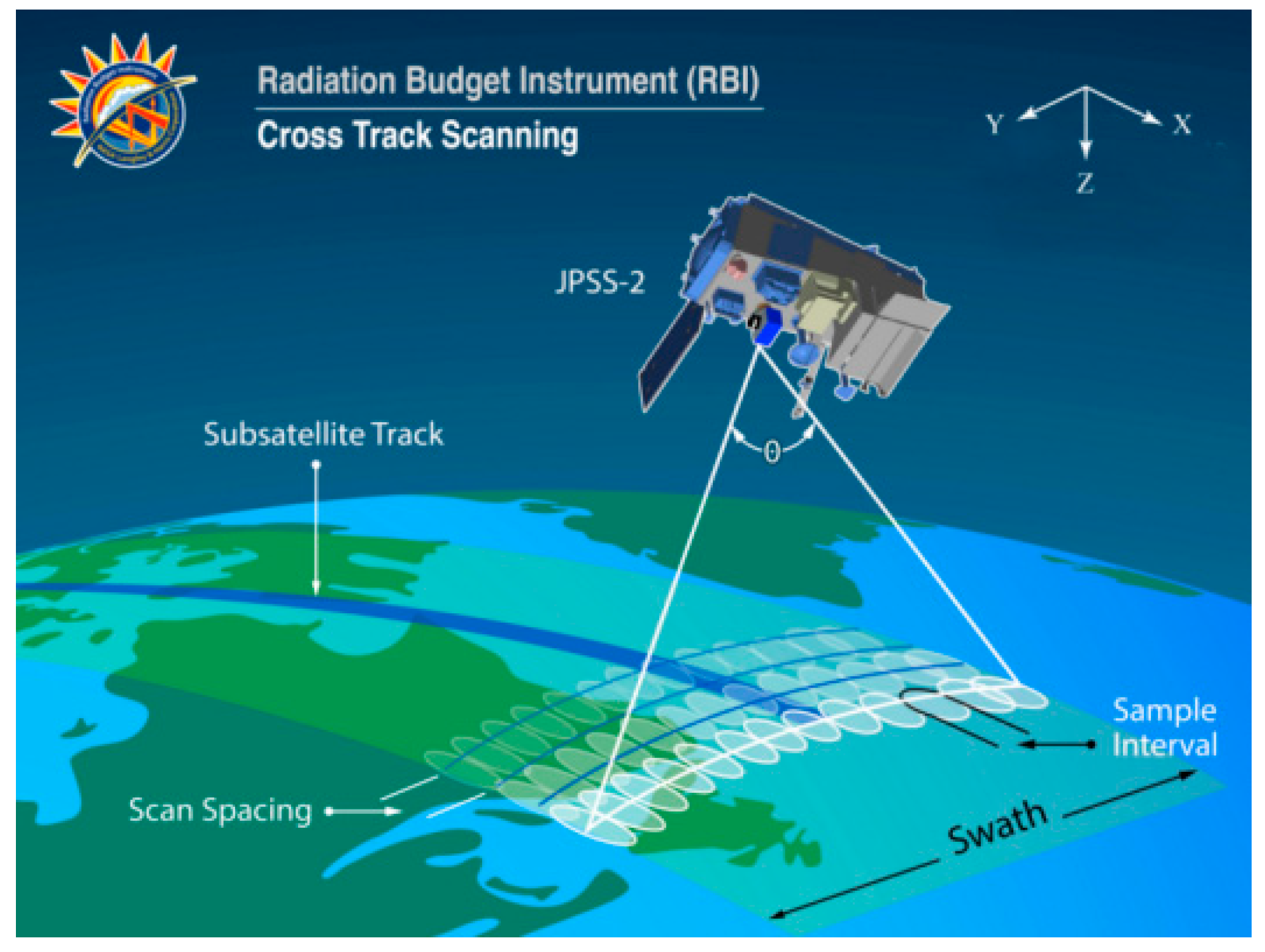
Traditional earth radiation budget (ERB) instruments such as those deployed on the Earth Radiation Budget Experiment (ERBE) [1] and on Clouds and the Earth’s Radiant Energy System (CERES) [2] and proposed for the ultimately deselected Radiation Budget Instrument (RBI) [3] consist of downward-looking telescopes in low earth orbit (LOE) which scan back and forth across the orbital path, as illustrated in Figure 1. While proven effective, such systems incur significant weight and power penalties and may be susceptible to eventual mechanical failure. Another approach to accomplishing the ERB mission is the Geostationary Earth Radiation Budget (GERB) instrument, which consists of a three-mirror imager illuminating a microbolometer focal-plane array (FPA) [4]. The ERB mission will also be assured by EarthCARE (earth, clouds, aerosols, and radiation explorer), which includes a Broadband Radiometer (BBR) suite consisting of three sets of two-dimensional paraboloid single-mirror optics, each illuminating a microbolometer linear array [5]. Both GERB and BBR rely on optical approaches to avoid scanning. In the case of GERB the field angle is limited by the extreme altitude of the instrument, which is parked in geostationary orbit. The narrow field angle significantly simplifies the optical design, and scanning is then achieved by the rotation of the Earth. The BBR suite on EarthCARE achieves optical simplification by push-broom operation and the use of a linear array; as in the case of scanning instruments, light gathering is limited to the width of a single pixel. The current contribution considers a novel approach in which a wide-field-angle imager is placed in LOE and the resulting astigmatism is corrected algorithmically.

Figure 2 is a CERES science product showing the monthly average global outgoing longwave radiation for May 2001 [6]. The CERES longwave channel is filtered to be sensitive only to earth-emitted radiation. The false-color map of monthly average band-limited flux (Wm⁻²) is relatively free of sharp edges and finely resolved features. This is equally true of the CERES shortwave channel, which is filtered to be sensitive only to earth-reflected solar radiation. The fact that scenes are effectively monochromatic and vary gradually within a given swath significantly limits their frequency content. A requirement of any next-generation staring imager is that it produces data products capable of mimicking those obtained from legacy scanners. In other words, images obtained must be relatable to the scanner footprints shown in Figure 1. Consequently, it is appropriate to represent earth scenes as consisting of a relatively modest number of directional beams.

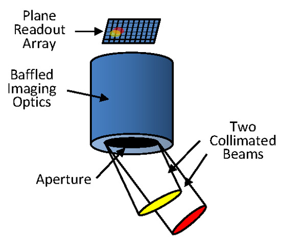
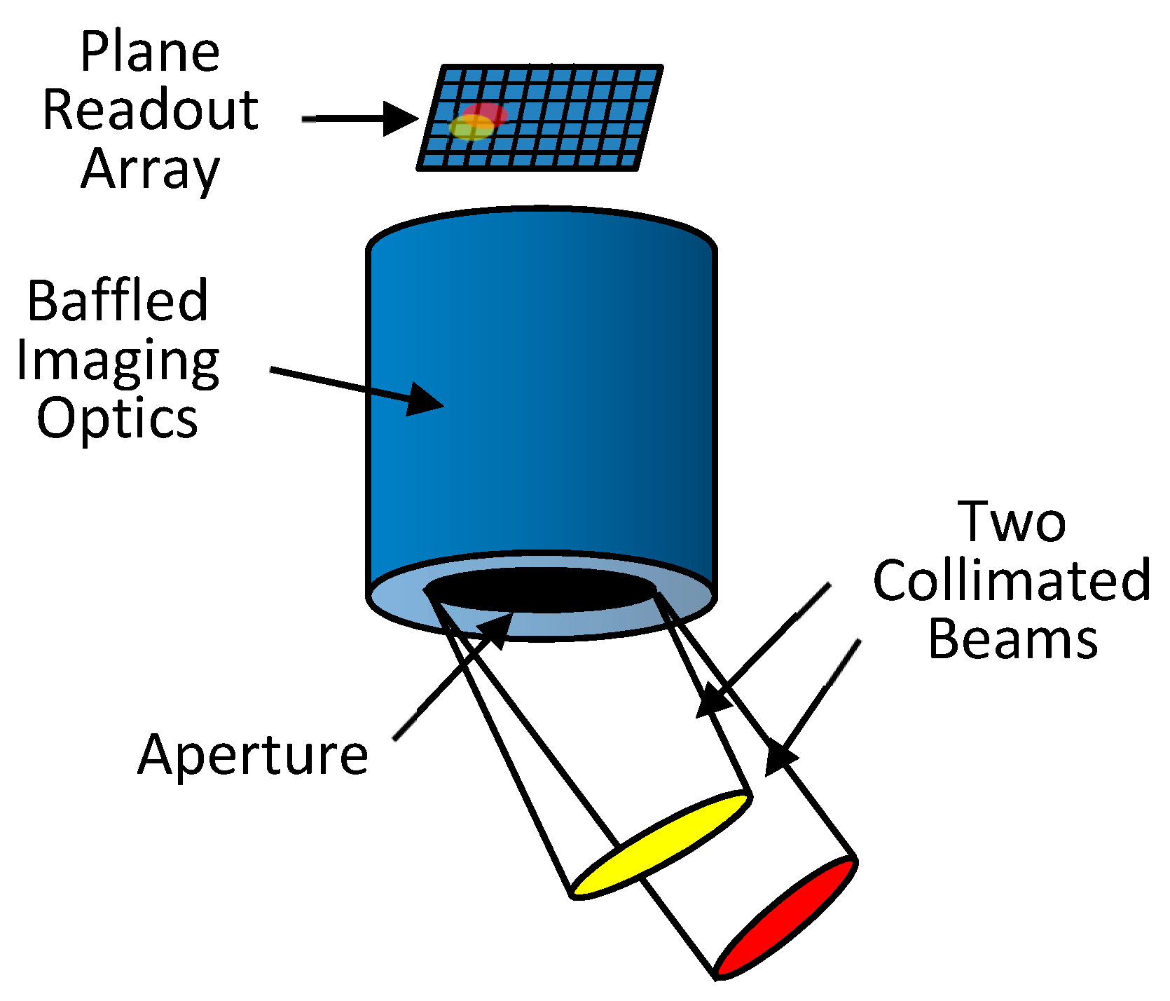
Figure 3 represents a generic wide-field-angle ERB imager consisting of an entrance aperture, baffled imaging optics, and a plane two-dimensional readout array. Two beams of radiation emanating from point sources at infinity are shown flooding the entrance aperture. Corresponding point-spread functions (PSFs) in the readout plane indicate the distribution of the beam energy there. Depending on the design of the optical train, focus will generally be achieved on a curved rather than on a plane surface. This is especially true when two-mirror optical systems of the Cassegrain or Ritchey-Chrétien type are pushed to their wide-field-angle limits. While deemed achievable, technology permitting non-planar microbolometer readout arrays has not yet been demonstrated. Therefore, we limit our consideration here to plane readout arrays, in which case blurring is expected to vary with field angle across the readout array. The challenge then is to create an accurate and computationally efficient algorithm for recovering the original discretized scene from the blurred illumination pattern on the readout array.

2. Image Deblurring

Following the formality of Pratt [7] the deblurring problem can be posed as

$$\begin{array}{cc}\hfill H f\left(x,y\right)& \equiv {{\displaystyle \int }}^{\text{}}{{\displaystyle \int }}^{\text{}}h\left(x-u,y-v\right)f\left(u,v\right)dudv=g_e\left(x,y\right)+n\left(x,y\right)\hfill \\ & \equiv g\left(x,y\right),\hfill \end{array}$$

(1)

where $f\left(x,y\right)$ is the deblurred image, $g_e\left(x,y\right)$ is the blurred image that would have been recorded in the absence of noise $n\left(x,y\right)$,$g\left(x,y\right)$ is the actual recorded image, $h$ is a point-spread function (PSF), and $H$ is an unknown matrix defined by the expression. In the discrete version of Equation (1) the double integral is replaced by a double sum over a discretized two-dimensional space. Then elements of the matrix $H_{ij}$ are sought such that

$$f_i=H_{ij}^{-1}{g}_j,$$

(2)

where the indices $i$ and $j$ represent ordered pixel numbers in a two-dimensional array. Then $f_i$ is the deblurred intensity of pixel $i$ and $g_j$ is the recorded intensity of pixel $j$. It should be emphasized that in discretized two-dimensional space both the deblurred image $f_i$ and the recorded image $g_j$ are defined by the same number of pixels; that is, $H_{ij}$ is a square matrix. While posed here as a problem in the space domain, practical implementation typically occurs in the frequency domain, in which case the Fourier transform dual of the PSF is the optical transfer function (OTF). Heuristically, deblurring involves deconvolution of either Equation (1), or its frequency-domain dual. In the case of non-blind deblurring, when the PSF (or OTF) is uniform and known across the image, the Lucy-Richardson algorithm [8,9] can be used to solve Equation (1). When the PSF is unknown it can often be reasonably modeled, for example as a Gaussian distribution having an unknown mean and variance. In this case the problem is ill-posed but can still be solved if an independent criterion for “good focus” is available against which the success of the solution can be evaluated. In such so-called blind deconvolution schemes a systemic search based on, for example, a genetic algorithm (GM) [10], can be conducted to identify the combination of deblurred images and uniform PSFs that best reproduces the recorded blurred image. Solutions obtained in this way are generally not unique but may still be useful. A viable alternative which assures stability and uniqueness is regularization [11]. Machine learning (ML) approaches to image deblurring have inevitably emerged, mostly in the context of improving PSF estimates [12,13,14,15,16].

Figure 4 is a scale drawing of a cross-section of a wide-field-angle Ritchey-Chrétien telescope (RCT) consisting of a field-limiting forward baffle, a baffled hyperbolic primary mirror, a baffled hyperbolic secondary mirror, and a plane readout array. A high-fidelity Monte Carlo Ray-Trace (MCRT) model of this instrument forms the basis for the current investigation. Ashraf et al. [17] have previously reported a novel approach to scene recovery by this instrument. In their previous approach a mean scene direction was computed for the rays absorbed on a given pixel of the readout array during simulated observation of a blackbody calibration source. A pixel-by-pixel calibration curve was then established by computing the corresponding absorbed power distribution on the readout array. This approach was shown to work well for the limited amount of testing to which it has been subjected.

The technique presented in the current contribution is similar to one described in Ref. [18], with the important difference that the authors of the cited reference start with a discretized well-focused image to which they add known mathematical noise and blurring. This is in contrast to our approach in which:

(1)

The readout array power distribution, which is the input to the ANN model, is produced by introducing a randomly discretized scene to the high-fidelity MCRT optical model of the imaging system, and

(2)

The readout array does not have the same number of pixels as the output of the ANN model, which represents the recovered discretized scene.

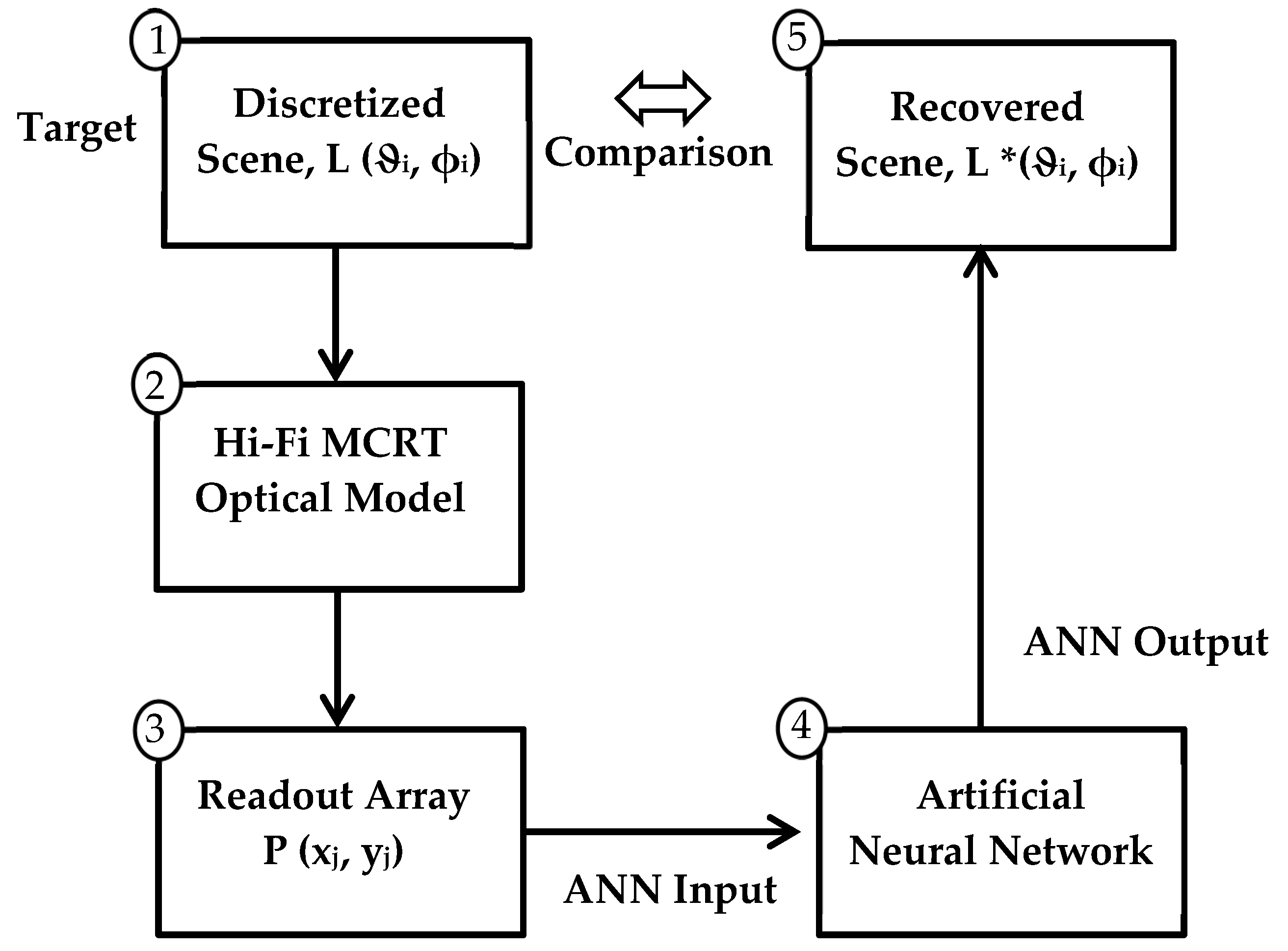
Rather than recording a replicate of the scene, the readout array is required only to record sufficient information to recover the original scene. Thus, our method is fundamentally different from the previous deblurring paradigms based on the solution of Equation (1). Instead, an artificial neural network (ANN) is used to characterize the relationship between the illumination pattern on the readout array and the corresponding discretized scene that produced it. The MCRT-based high-fidelity model (HFM) of the imager is used to train the ANN by presenting it with a large number of pairs of readout array power distributions and corresponding discretized scene intensity distributions. Once trained, the ANN may then be used to predict the discretized scene corresponding to any recorded readout array power distribution. The logic flow of the technique is illustrated in Figure 5.

Step 1. Creation of Scene/Readout array Pairs

Block 1 in Figure 5 indicates a process in which scenes are synthesized as a collection of random-strength beams incident from a discrete set of directions. Each beam, representing light from a point source at infinity, consists of a large number of parallel rays that flood the entrance aperture of the high-fidelity Monte Carlo Ray-Trace (MCRT) imager model of the telescope shown in Figure 4 and represented by Block 2 in Figure 5. Details of the imager model are similar to those elaborated in Chapter 3 (pp. 85–94) of Ref. [19]. Block 3 records the output of the imager high-fidelity model (HFM) on a plane two-dimensional 19 × 19-pixel readout array. During Step 1, 2000 random-strength beams incident from 50 specified directions are input to the imager HFM, producing 2000 corresponding power distributions on the readout array.

Step 2. Training the Artificial Neural Network (ANN)

A random selection of 1950 of the 2000 readout array power distributions created in Step 1 and loaded into Block 3 are input one at a time into the artificial neural network represented by Block 4. For each of these readout array power distributions, the synaptic weights of the ANN are adjusted in an iterative process, described in Section 4, which minimizes the difference between the ANN output scene represented by Block 5 and the corresponding target scene in Block 1.

Step 3. Testing the Artificial Neural Network

The 50 readout array power distributions created in Step 1 that were not used to train the ANN in Step 2 are introduced sequentially into the trained ANN. Then the resulting output scene (Block 5) in each case is compared to the target scene (Block 1) used to create it. The pixel-by-pixel differences between corresponding ANN output and target scenes are a measure of the success of the proposed numerical focusing scheme.

Step 4. Prediction of unknown scenes from recorded readout array power distributions

Availability of a properly trained and tested ANN model of the imager renders further ray tracing unnecessary. From this point forward, the trained ANN model can be reliably used to convert recorded readout array power distributions to corresponding discretized scenes by following the path Block 3→Block 4→Block 5. Alternatively, the operational instrument, once built, can be calibrated by introducing discrete beams from collimated sources incident from directions corresponding to the desired directional resolution. Preliminary versions of the ANN model can be used in the design phase of instrument development, while higher-order, more refined models can be used to yield scientifically accurate science data during on-orbit operation of the actual imager.

Details of the individual steps are provided in Section 3, Section 4 and Section 5.

3. Instrument Model

The specific Ritchey-Chrétien telescope (RCT) which informs the current investigation is shown in Figure 4. The three ray-traces shown indicate that beams entering at different field angles achieve focus on a curved surface (the dashed curve). Therefore, the PSF of a beam on the plane readout array will be increasingly misfocused with increasing incidence angle. While the results reported in the current investigation are specific to this particular optical system, the methodology used to obtain them is general and therefore applicable to virtually any optical system for which a high-fidelity performance model is available.

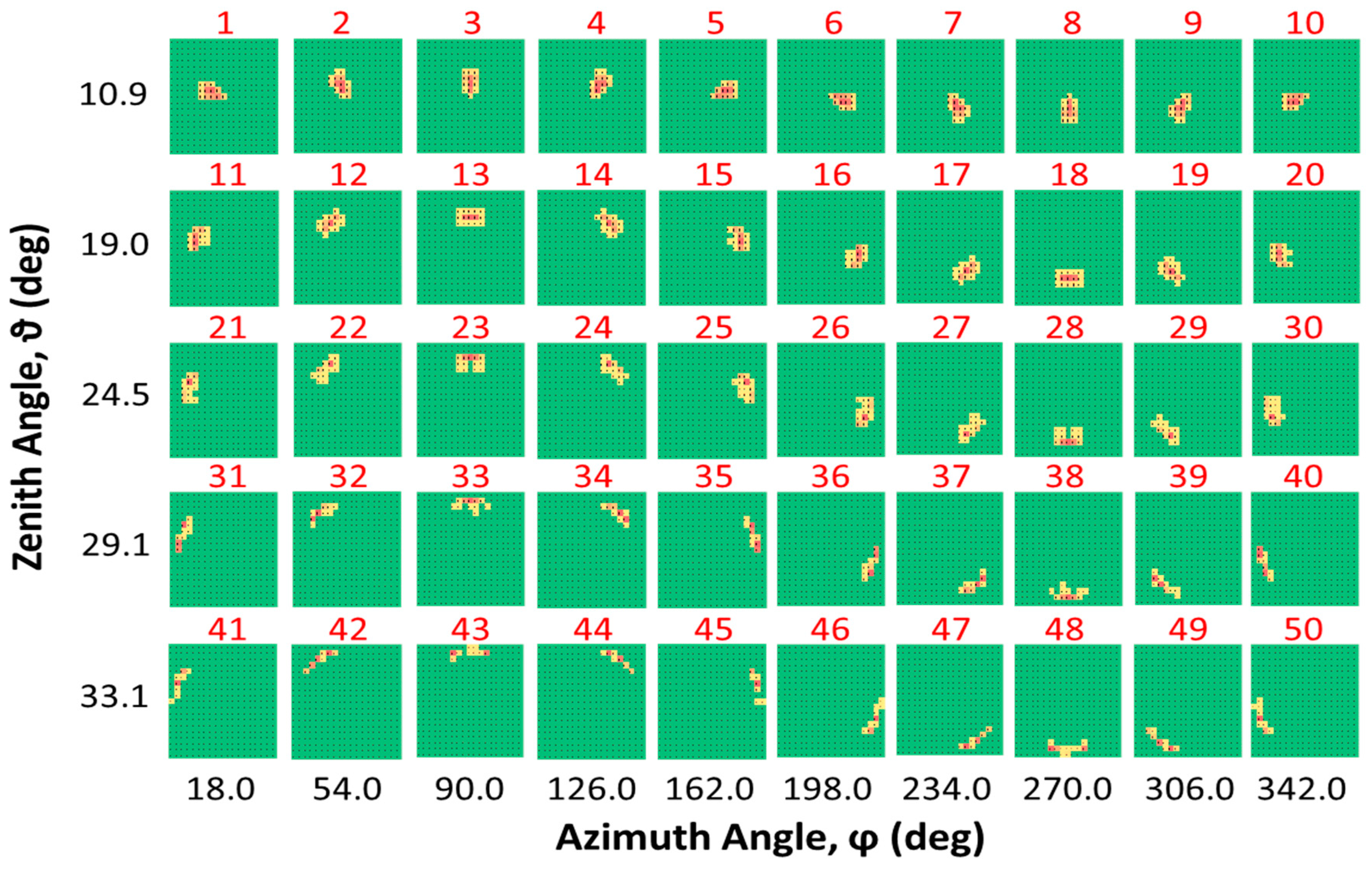
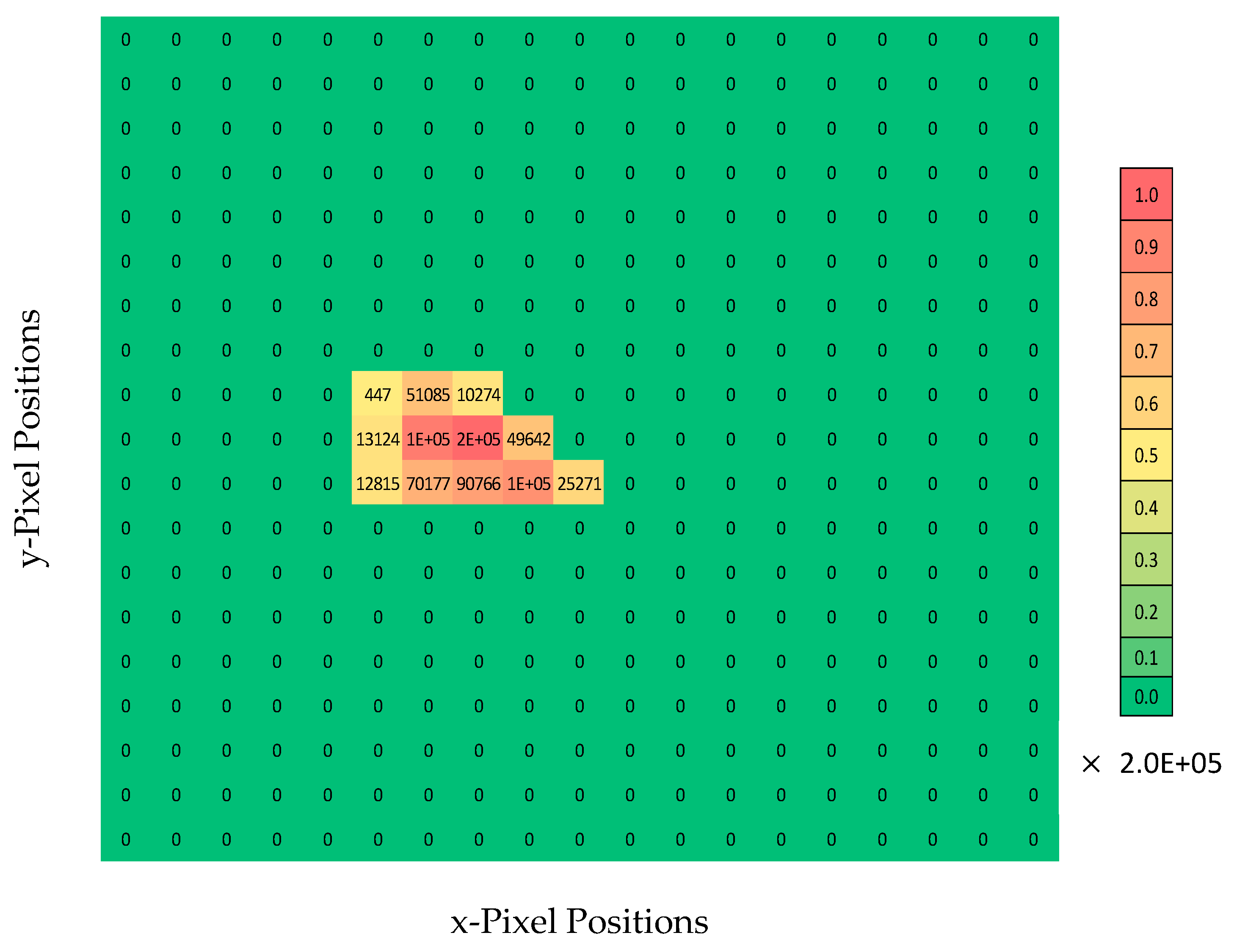
A Monte Carlo ray-trace [19] is performed in which millions of rays are traced from each of 50 directions to form beams, each flooding the entrance aperture of the telescope shown in Figure 4. Following Ashraf [20], the 50 directions are determined by first dividing an imaginary hemisphere surmounting the entrance aperture into equal-area sectors. Then the rays forming a given beam are constrained to pass parallel to a ray which passes normal to the centroid of one of the sectors. The rays are traced through the baffled telescope and eventually absorbed on a 361-pixel two-dimensional microbolometer array. Results of a ray-trace for a one-million-ray beam incident to the aperture at a zenith angle ϑ of 10.9 deg and an azimuth angle ϕ of 18.0 deg are shown in Figure 6, and results for all 50 beams showing the distribution of absorbed power from each of the 50 directions on the 19-by-19-element array are given in Figure 7. Each incident beam direction is assigned a number ranging from 1 to 50. Assigned beam numbers are indicated in red type. In Figure 6 and Figure 7, the red end of the color spectrum represents the largest number of rays absorbed by a pixel for a given direction, and the yellow end of the spectrum represents the smallest nonzero number of absorbed rays, with green indicating zero rays. Creation of the fifty “primitives” shown in Figure 7 required about 250 min of machine time on a laptop PC.

It is clear from inspection of Figure 6 that power from beams incident from a given direction is absorbed by several neighboring pixels. The distribution becomes increasingly distorted moving from $\vartheta$ = 10.9 to $\vartheta$ = 33.1 deg for a given value of $\phi$. Also, the number of rays in the original beam that reach the readout plane decreases with zenith angle.

4. The Artificial Neural Network

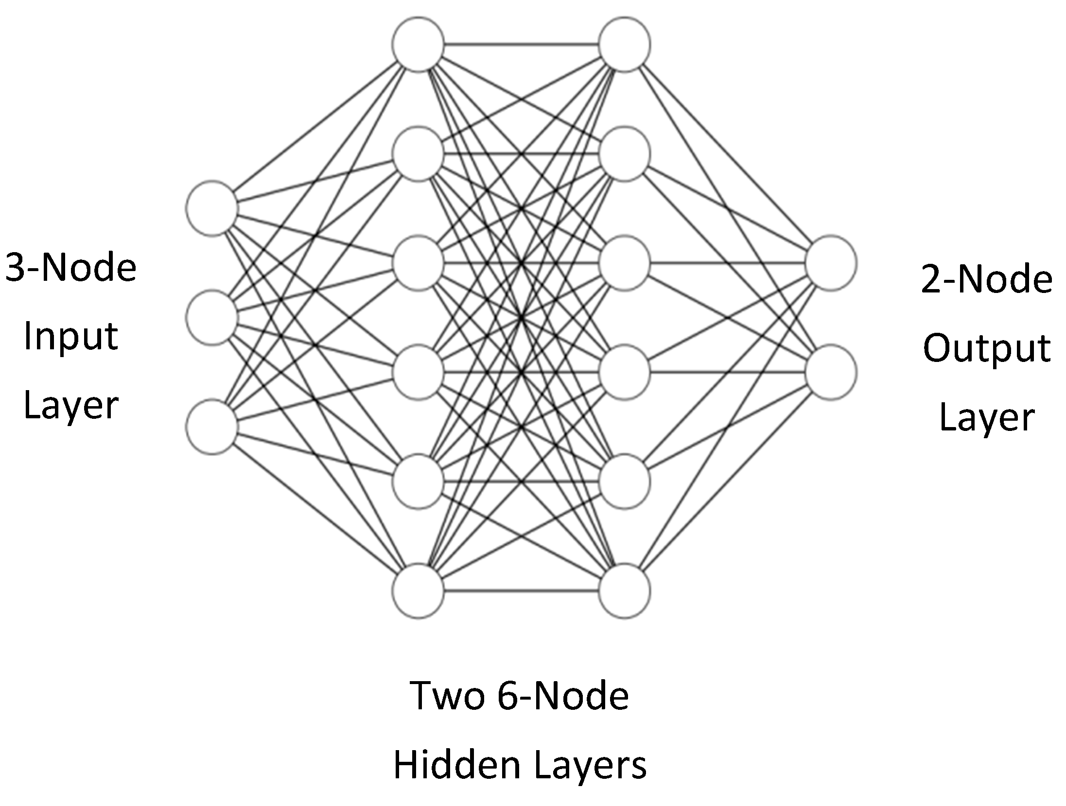
An artificial neural network (ANN) is an information-processing paradigm inspired by the biological neuron system found in the human brain. It consists of a large number of simple processing elements called neurons, or nodes, organized in layers, as illustrated in Figure 8. In a fully-connected ANN, all nodes of each hidden layer communicate with all nodes of the previous and following layers by means of synaptic connectors. Each connector is characterized by a synaptic weight. The values in the output layer characterize the response of the system to the values in the input layer. In the current application the input layer consists of 361 nodes describing the power distribution on the readout array, and the output layer consists of 50 nodes describing the corresponding intensities of the beams incident to the instrument aperture. While the configuration shown in Figure 8 illustrates a 3-node input layer, two 6-node hidden layers, and a 2-node output layer; the ANN created for the current application features a 361-node input layer, two 100-node hidden layers, and a 50-node output layer.

The synaptic weights determine the relative importance of the signals from all the nodes in the previous layer. At each hidden-layer node, the node input consists of a sum of all the outputs of the nodes in the previous layer, each modified by an individual interconnector weight. At each hidden node, the node output is determined by an appropriate activation function, which performs nonlinear input-output transformations. The information treated by the connector and node operations is introduced at the input layer, and this propagates forward toward the output layer [21]. Such ANNs are known as feed-forward networks, which is the type used in the current study.

The output layer error can be determined by direct comparison between the recovered scene (Block 5 in Figure 4) and the target discretized scene (Block 1 in Figure 4). Training of the ANN adjusts its synaptic weights to minimize the errors between these two images. The training procedure for feed-forward networks is known as the supervised back propagation (BP) learning scheme, where the weights and biases are adjusted layer by layer from the output layer toward the input layer [22]. The mathematical basis, the procedures for training and testing the ANNs, and a fuller description of the BP algorithm can be found elsewhere [23].

Overfitting may occur because of an overly complex model with too many parameters. A model that is overfitted is inaccurate because the trend does not reflect the reality present in the data. The presence of overfitting can be revealed if the model produces good results on the seen data (training set) but performs poorly on the unseen data (test set). This is a very important consideration since we want our model to make predictions based on the data that it has never seen before. Therefore, in the current application, additional structured test scenes were introduced involving data completely unknown to the ANN training process. As shown in Section 5, the trained model performed extremely well on them. We take this as an indication that we do not have the problem of overfitting in our model and that it can generalize well from the training data to any data from the problem domain. Techniques such as early stopping, data augmentation, regularization, and drop-out are available to overcome this problem if detected.

An Adam optimization algorithm is used in the present study to converge the ANN output with the target scenes during the training process. This stochastic optimization method is straightforward to implement, is computationally efficient, has little memory requirements, is invariant to diagonal rescaling of the gradients, and is well suited for problems that are large in terms of data. Further details about Adam optimization can be found in Ref. [24].

Mean-squared error (MSE) is used as the objective loss function for the ANN optimization. An inherent weakness of the BP algorithm is that it can converge to a local minimum. One way to avoid this tendency is to change the learning rate during the network training process. “Learning rate” refers to the rate of change of the neural network weights during optimization. The learning rate was ultimately set to 0.0002. Training of the neural network is terminated when a predetermined maximum number of training cycles have been completed. Selection of the maximum number is a trial-and-error process in which the number may be changed if the performance of the neural network during initial training falls short of expectations. In the current study 40,000 iterations were found to produce good results.

The relative error of predicted output $i$ is defined by

$$R{E}_i= \frac{\left|targe{t}_i-outpu{t}_i\right|}{targe{t}_i},$$

(3)

where $outpu{t}_i$ is the scene intensity predicted by the ANN, and $targe{t}_i$ is the corresponding known scene intensity. In the current investigation, performance is evaluated by calculating the mean value of the relative error,

$$MRE=\frac{1}{n}{\displaystyle \sum }_{i=1}^{n}R{E}_i,$$

(4)

where $n=50$ for the predicted 50 incident directions in the scene.

An a priori selection of ANN hyperparameters such as network topology, training algorithm, and network size is usually made based on experience. After training, the final sets of weights and biases trained by the network can be used for prediction purposes, and the corresponding ANN becomes a model of the input/output relation of the given problem.

5. Implementation and Results

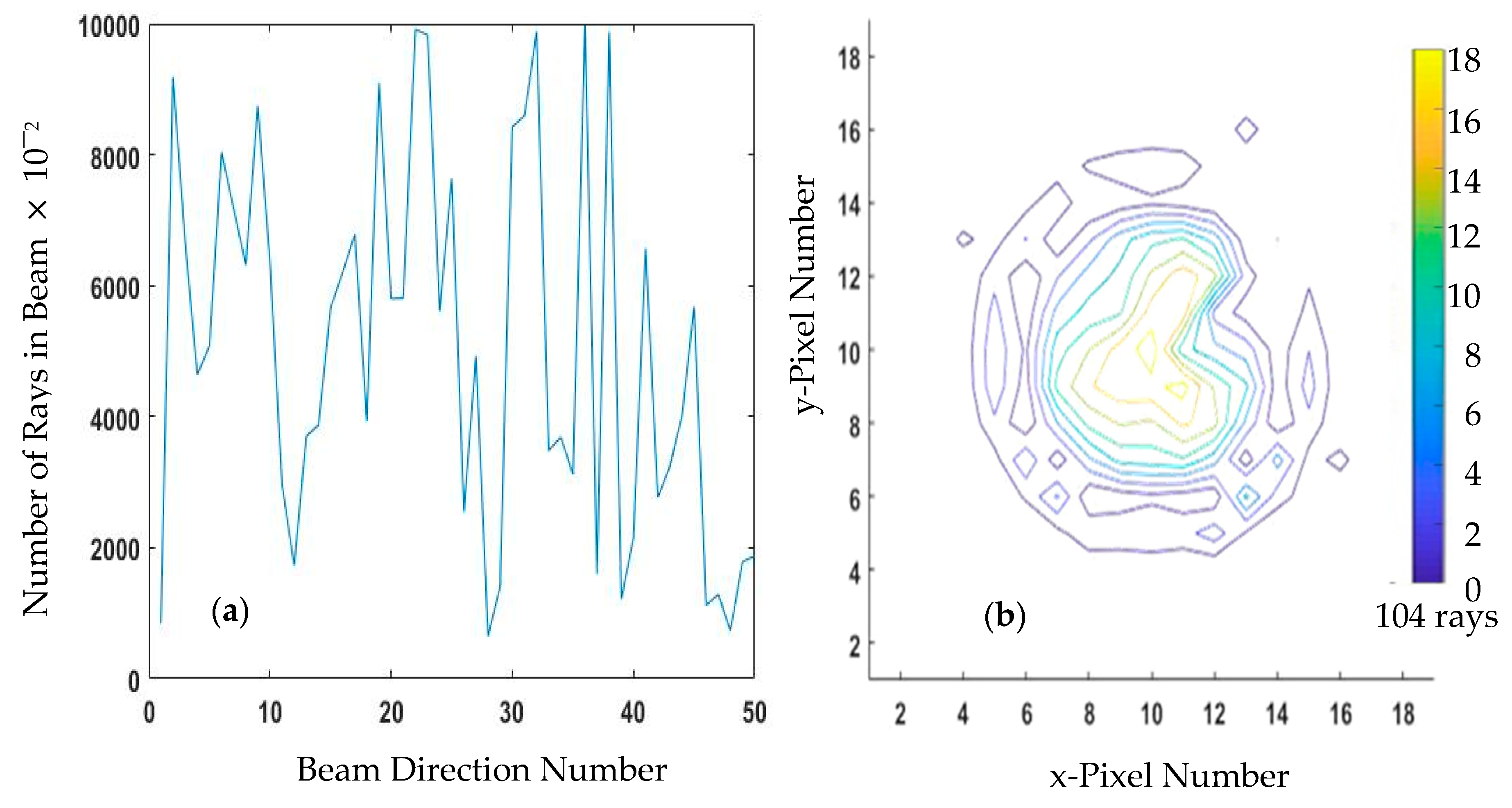
We create 2000 discretized scenes by combining the 50 primitive beam illumination patterns in Figure 7 after first multiplying each of them by a random scaling factor representing the relative scene intensity corresponding to each direction. This produces a set of 2000 readout array power distributions corresponding to the 2000 scenes viewed by the instrument. Figure 9a shows a typical scene intensity distribution and Figure 9b shows the corresponding distribution of rays on the readout array. Even though the ray distribution in Figure 9b is produced by the single random scene in Figure 9a, essential features of the optical system are already readily apparent.

We randomly select 1950 of the 2000 readout array/incident-scene pairs to train the ANN. Each of the 1950 361-pixel readout array power distributions is input to the ANN with the goal of reproducing the target 50-element scene. The training process uses the optimization algorithm outlined in Section 4 to automatically adjust the synaptic weights of the ANN to minimize the global difference between the 1950 target scene intensity distributions and the 1950 scene intensity distributions returned by the ANN. It is emphasized that the ANN is used to solve the inverse problem directly based on the data obtained from the solution of the forward problem using a high-fidelity MCRT model.

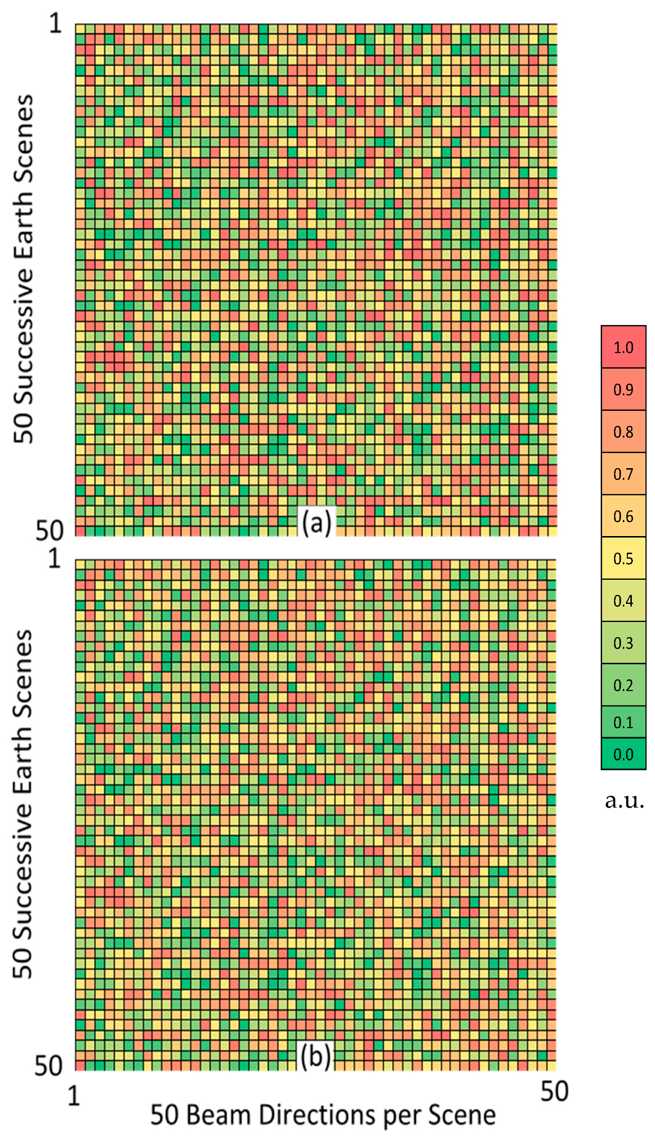
We first test the ANN (i.e., establish its accuracy) by introducing the 50 sets of readout array power distributions not already used for training into the trained ANN to produce 50 test scenes. We then compare the test scenes created by the ANN with the corresponding target scenes. Figure 10 uses color variations to represent the fifty test “Earth” scenes and the corresponding scenes obtained using the ANN. In the figure, the red end of the color spectrum represents higher intensity and the green end represents lower intensity. While the similarity between Figure 10a and b is evident, with many red and green groupings being clearly identifiable in both, it is also possible to visually discern differences.

Figure 11 shows the direction-by-direction percentage difference in the scenes in Figure 10a,b. In the figure, the green cells indicate percentage differences of less than ±1.0%, and the pink cells indicate differences of greater than ±1.0%. Although the font size in the figure makes individual numbers difficult if not impossible to read, most of the pink cells in the left-hand third of the figure show values of less than two percent, while a few of the pink cells in the right-hand third show values exceeding 100 percent. The left-to-right degradation of the ANN scene-recovery accuracy is attributable to the declining signal strength with increasing beam number. This conclusion is justified by reference to Figure 9b, which clearly shows the roll-off of absorbed power with distance from the center of the readout array, and to Figure 7, which shows that Beams 41 through 50 are responsible for illuminating the outer edges of the array.

The randomness and unordered sequencing of the 50 scenes used to produce Figure 10 and Figure 11 make it difficult to visually assess the remarkable potential of numerical focusing based on artificial neural networks. A clearer demonstration of its potential is obtained based on the ordered sequence of fifty scenes shown in Figure 12a. In the figure each of the fifty scenes, or horizontal strips, can be thought of as emanating from a swath of the earth that might correspond to an appropriate number of successive RBI scans illustrated in Figure 1. Figure 12a would then be the result obtained by assembling the fifty RBI-like footprints into an earth-emitted or earth-reflected solar image of a region of a notional Earth. Figure 12b is the assembled sequence of 50 scenes produced by the ANN when the 50 readout array power distributions corresponding to the 50 scenes in Figure 12a are input to the ANN.

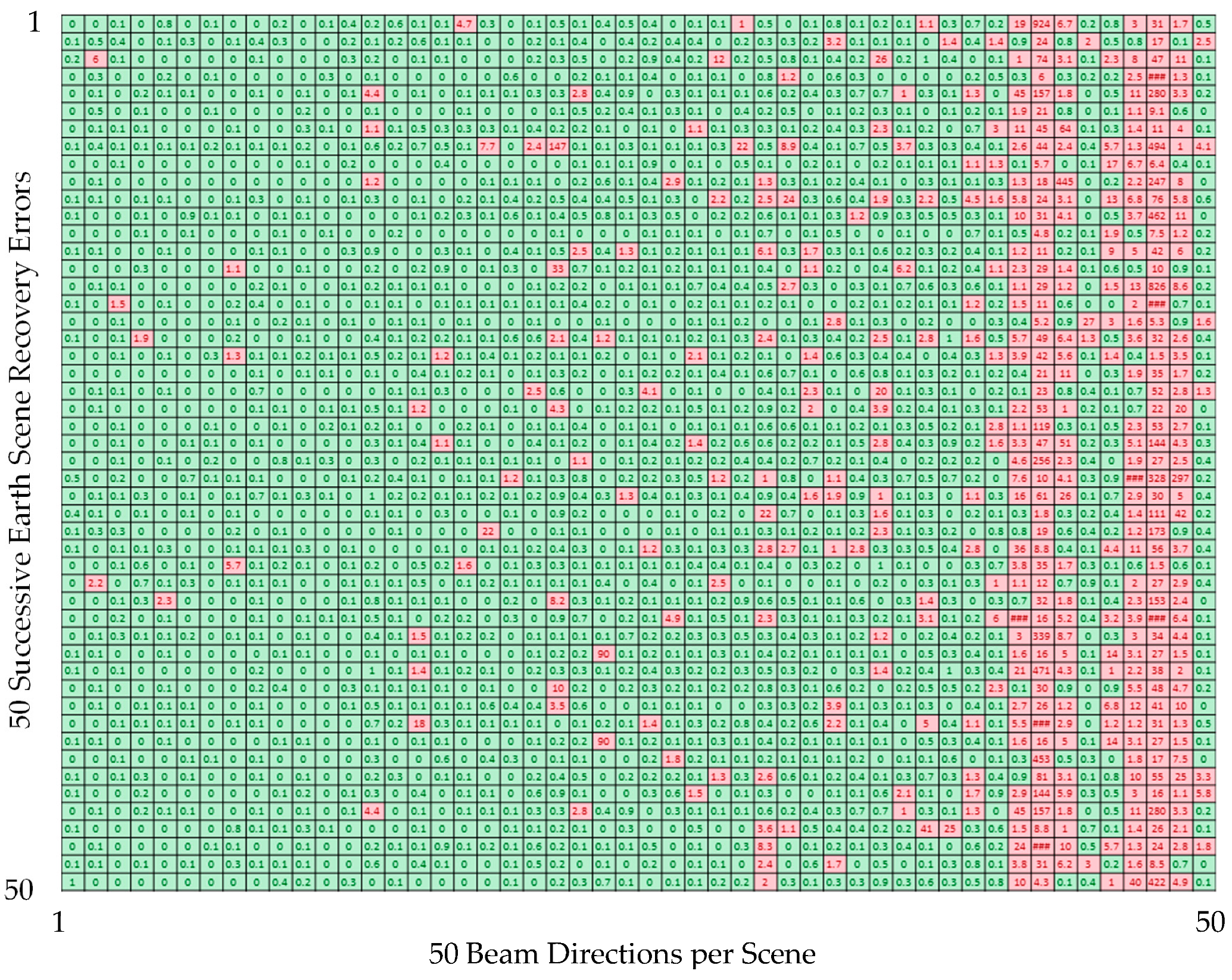
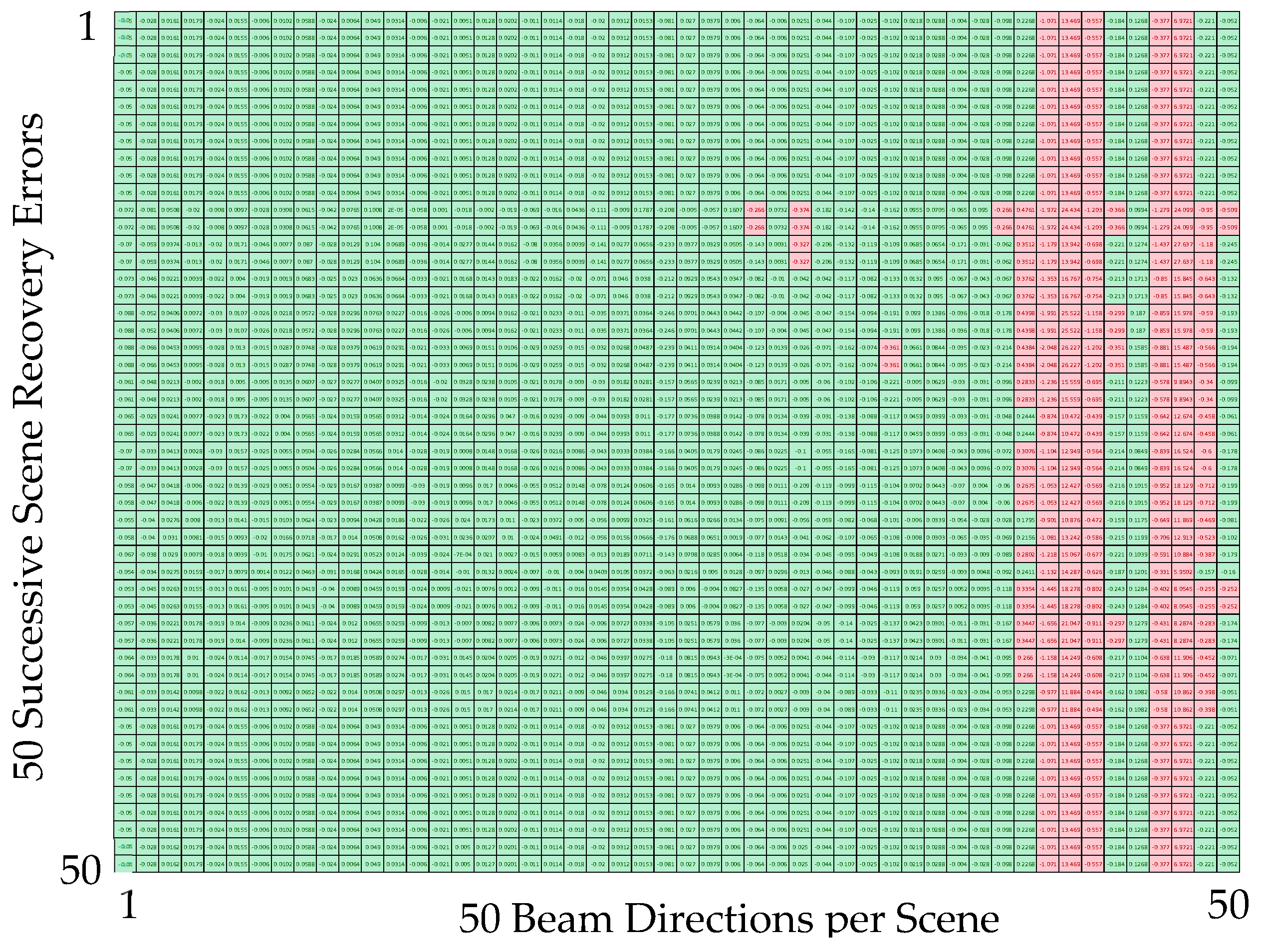
The scene recovery error associated with a low signal-to-noise ratio in the final ten beam directions is apparent in the right-most portion of Figure 12b. Otherwise the ability of the ANN numerical focusing scheme to accurately recover the incident scene from the defocused readout array power distribution is well demonstrated. Figure 13 shows the direction-by-direction percentage difference in the scenes in Figure 12a,b. In the figure, the green cells indicate percentage differences of less than ±0.25%, and the pink cells indicate differences of greater than ±0.25%. The ability of the ANN to produce results that are consistently within one-quarter of a percent of the actual scene when the scene is so dissimilar to the 2000 random scenes used for training and testing is evidence of strong generalization and a low likelihood of overfitting.

6. Summary and Conclusions

Results of the proof-of-concept investigation reported here are limited to scenes consisting of 50 directionally incident beams imperfectly focused onto a 361-pixel microbolometer array. No attempt has been made to optimize or otherwise improve the results by increasing the directional resolution of the scene or the spatial resolution of the readout array. Even using these relatively coarse scene and readout array resolutions, we are able to obtain scene recovery accuracy at the sub-one-percent level over the center portion of the telescope field-of-view using an artificial neural network. An implication of the effort reported here that should not be overlooked is that, once an ANN has been trained on the basis of a high-fidelity MCRT model of the optical system, the much faster low-order model can be used in subsequent performance evaluation of the system with a significant reduction in computer resources. This means that the actual instrument, once accurately modeled, can provide on-orbit earth radiation scene observations in real time. An alternative to relying upon the high-fidelity MCRT model to tune the ANN model would be preflight calibration of the actual instrument. This would involve the use of a steerable beam light source of known intensity in a thermal-vacuum chamber.

During on-orbit operation the elements of the two-dimensional readout array would be time-sampled to obtain a sequence of intensity distributions incident to the imager entrance aperture from the discrete directions for which it was trained. The inverse optical model is sufficiently fast to obtain these images in real time. Note that the image obtained is discretized even though the scene being observed is continuous, as is true in the case of any imager based on an ordinary focal-plane array (FPA). However, in this case the number of scene pixels—fifty in the current application—is generally different from the number of FPA pixels—361 in the current application. In a future effort the relationship between these two numbers will be studied in an effort to maximize the accuracy of the method.

We conclude that ANNs offer a viable means for creating computationally efficient models of complex optical systems from computationally intensive high-fidelity models based on the MCRT method. Specifically, while the MCRT method requires more than four hours to solve the forward problem of readout array illumination, the solution, once obtained, may be used to train an ANN to solve the much more interesting inverse problem of recovering the incident scene in real time.