DEM Extraction from ALS Point Clouds in Forest Areas via Graph Convolution Network


1
School of Remote Sensing and Information Engineering, 129 Luoyu Roud, Wuhan University, Wuhan 430079, China
2
Institute of Land Resource Surveying and Mapping of Guangdong Province, 28 North Wuxianqiao Street, Guangzhou 510500, China
*
Author to whom correspondence should be addressed.
Remote Sens. 2020, 12(1), 178; https://0-doi-org.brum.beds.ac.uk/10.3390/rs12010178
Submission received: 21 November 2019
/
Revised: 10 December 2019
/
Accepted: 20 December 2019
/
Published: 3 January 2020
Abstract
:It is difficult to extract a digital elevation model (DEM) from an airborne laser scanning (ALS) point cloud in a forest area because of the irregular and uneven distribution of ground and vegetation points. Machine learning, especially deep learning methods, has shown powerful feature extraction in accomplishing point cloud classification. However, most of the existing deep learning frameworks, such as PointNet, dynamic graph convolutional neural network (DGCNN), and SparseConvNet, cannot consider the particularity of ALS point clouds. For large-scene laser point clouds, the current data preprocessing methods are mostly based on random sampling, which is not suitable for DEM extraction tasks. In this study, we propose a novel data sampling algorithm for the data preparation of patch-based training and classification named T-Sampling. T-Sampling uses the set of the lowest points in a certain area as basic points with other points added to supplement it, which can guarantee the integrity of the terrain in the sampling area. In the learning part, we propose a new convolution model based on terrain named Tin-EdgeConv that fully considers the spatial relationship between ground and non-ground points when constructing a directed graph. We design a new network based on Tin-EdgeConv to extract local features and use PointNet architecture to extract global context information. Finally, we combine this information effectively with a designed attention fusion module. These aspects are important in achieving high classification accuracy. We evaluate the proposed method by using large-scale data from forest areas. Results show that our method is more accurate than existing algorithms.

1. Introduction
Airborne laser scanning (ALS) point cloud processing has been performed for the last two decades [1]. An ALS point cloud has three-dimensional (3D) geometric information with intensity and multiple returns, making the approach suitable for collecting high-quality topographic data in forest areas. Eliminating or filtering non-ground points is the key to generating a digital elevation model (DEM) from the ALS point cloud. In forest areas, the ground points collected by ALS can be extremely sparse, thus possibly complicating automatic filtering due to insufficient information. How to extract DEMs from ALS point clouds effectively is a big challenge that has brought much attention in recent years.
There are many classic methods in DEM extraction based on handcrafted algorithms. These methods classify point clouds by designing rules, feature representations, and characteristics of points with different categories, including progressive triangulation [2], slope analysis [3,4], surface-based methods [5,6,7,8], mathematical morphology [9], and optimization-based method [10,11], which have been used in software such as TerraSolid and CloudCompare. Also, these methods were integrated into open-source libraries for point clouds, such as the Point Cloud Library (PCL). Handcrafted algorithms can be parameter- or setting-sensitive and are suitable for simple scenes. However, forest scenes are complex and variable without fixed features, therefore, it is difficult to design appropriate feature parameters to guarantee the robustness of these algorithms.
To increase the robustness of the algorithms, many scholars studied point cloud classification by machine learning, such as support vector machine (SVM) [12], random forest (RF) [13], and AdaBoost [14]. Chehata et al. [15] proposed a framework that applied an RF classifier to classify full-waveform point cloud data. The advantage of this method is that it cannot only deal with all types of full-waveform attribute features but also obtains accurate results by using an RF classifier and runs efficiently on large datasets. To solve the multi-class problem, Mallet et al. [16] designed a multiclass SVM to classify point clouds in urban areas. Similarly, Kim et al. [17] proposed a power line classification method for a point cloud based on an RF classifier. This method trains an RF classifier by using approximately 30 manual features extracted from point, line, and surface regions. To further improve the classification effect, Kang et al. [18] proposed a point cloud classification method based on a Bayesian network, which combines the geometric features of point clouds and the spectral features of images, to classify ground, vegetation, and building points in a survey area. Zhang et al. [19] trained an AdaBoost classifier by using multiscale geometric features to classify trees, buildings, and vehicles. However, the above classification methods, which are based on local features, ignore context relationships among classification units, resulting in local errors, such as random noise, in the classification results. To solve this problem, the Markov random field [20,21,22] and conditional random field (CRF) [23,24,25] use a spatial context information model for classification and achieve satisfactory results. Furthermore, Niemeyer et al. [26] combined RFs and CRFs to classify point clouds.
In recent years, deep convolutional neural networks (DCNNs) have been applied to point cloud processing. In comparison with handcrafted algorithms, deep learning-based methods learn features automatically and can obtain low error rates. Hu and Yuan [27] applied a DCNN to filter ALS point clouds. In their method, the classification of a point is treated as the classification of an image mapped from the elevation distribution of point neighbors. The method exhibits good accuracy but runs slowly and is problematic in forest areas.
DCNN-based methods have the following basic frameworks for point cloud processing: multi-view-based [28], voxel-based [29,30], and point-based [31,32] networks. Deep learning was first applied to image processing tasks and could not be applied in point clouds. Therefore, in [28], the point cloud was converted into multi-view images, and the image classification network was used to classify point clouds. However, in the process of multi-view image generation of the point cloud, there was an occlusion situation, which made it difficult to apply it to the point cloud segmentation task. To solve this problem, in [29,30], the point clouds were converted into a 3D voxel space, and the voxel was processed using a 3D convolutional neural network. These methods can effectively complete the point clouds segmentation task, but compared with two-dimensional (2D) dimensional convolution, 3D convolution takes more graphics processing unit (GPU) memory and longer running time. Also, the effects are influenced by the resolution of the voxel. To further improve the quality of point cloud processing, in [31,32], the point cloud was directly processed, and point cloud processing frameworks PointNet and PointNet++ were proposed. These two frameworks greatly promote the development of deep learning in point clouds. Point-based methods directly process point clouds, so they avoid possible problems in transferring points into images or voxels used in multi-view- and voxel-based networks. After that, many point-based deep learning frameworks were proposed. PointCNN [33] used learning as an X-transformation from the input points to promote two causes simultaneously. The first cause is the weighting of the input features associated with the points, while the second cause is the permutation of the points into a latent and potentially canonical order. However, this process relies heavily on the color and intensity of point clouds. Rethage [34] proposed a general and fully convolutional network architecture to process large-scale 3D data efficiently. Jiang et al. [35] designed a module called PointSIFT, which encoded information of different orientations and adapted to the scale of a shape. With the development of graph convolution neural network (GCNN), many studies had applied the GCNN model to process point clouds. Wang et al. [36] processed a point cloud using a dynamic GCNN, which fully explored the local spatial relations and information of any spatial distribution of points. Te [37] proposed a regularized GCNN (RGCNN), which directly consumed point clouds. To process large-scale point clouds, Landrieu [38] proposed a novel deep learning-based framework called super point graph to solve the challenge of semantic segmentation. GCNN has great advantages in describing the spatial distribution of a point cloud and is more efficient than voxel- and multi-view-based frameworks. When processing forest areas, GCNN is beneficial for enhanced representation of the features of sparse ground points and complex terrains with steep slopes.
To further improve the effect on ALS point cloud DEM extraction, in this study, we propose a novel data preprocessing method based on a terrain model named T-Sampling and a new TinGraph-Attention network to extract ground points. The input point clouds are divided into multiple patches, with each patch consisting of basic and additional points. After gridding, we extract the lowest point in each grid from the point cloud as the basic point and randomly combine the remaining points with the basic points as input blocks. These blocks are the input of the proposed network. Our network contains three parts: local feature extraction, global feature extraction, and feature fusion. In the local feature extraction part, we propose a Tin-EdgeConv layer to compute the local features of each point. In the global feature extraction part, we use the basic PointNet model to extract the global features of the input point cloud. In the feature fusion part, we use an attention fusion module to fuse local and global features. We evaluate our method using complex forest areas. The experimental results show that our method is superior to other state-of-the-art algorithms.
We explicitly state our original contributions as follows.
- (1)
- We propose a triangulated irregular network (TIN)-based random sampling method named T-Sampling that can ensure the terrain information of each input patch to avoid terrain expression loss caused by random sampling. Simultaneously, the original input point cloud is divided into several parts. Finally, the classification results of the original point are obtained by weighting and summing the network prediction results of each part.
- (2)
- To express the terrain information in the graph convolution layer, we propose a Tin-EdgeConv layer to enhance the extraction of terrain information. The proposed layer ignores the traditional nearest-neighbor features in the point cloud but focuses on the nearest-neighbor feature of the triangulated irregular network formed by the topography.
- (3)
- We propose a TinGraph-Attention network to consider additional contextual information into the point cloud classification. The proposed Tin-EdgeConv layer can describe the local terrain features of the point clouds well. Combined with the global features extracted by PointNet through the attention fusion model, the local features will be complete, thus possibly improving the classification results.
The remainder of this paper is organized as follows. Section 2 presents the components of our proposed framework. Section 3 reports the extensive experimental results and evaluates the performance of the proposed method. Section 4 presents the discussion. Finally, Section 5 provides the conclusions and hints at plausible future research.
2. Methodology
2.1. Overview of the Proposed Framework
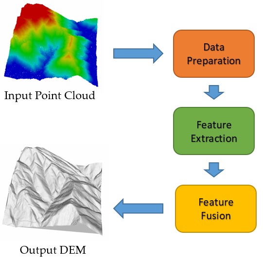
Our proposed framework is divided into three stages: data preprocessing, feature extraction, and feature fusion. As shown in Figure 1, a row of point clouds at the data preprocessing stage is sampled to many pieces, with each piece containing the same ground feature points and different additional points. After data preprocessing, the feature extraction stage consists of the extracted local features, and global feature extraction is applied to extract the features at different levels. At the feature fusion stage, the two kinds of features are fused by an attention fusion module, which preserves the detailed information described by the local features. The final result of the input point clouds is weighted by the class probability of each piece.
The input point clouds are denoted by , where . In our network, only the geometric information of the point cloud is used; that is, the intensity, red/green/blue (RGB), and other information are neglected.
2.2. Data Preprocessing Algorithm
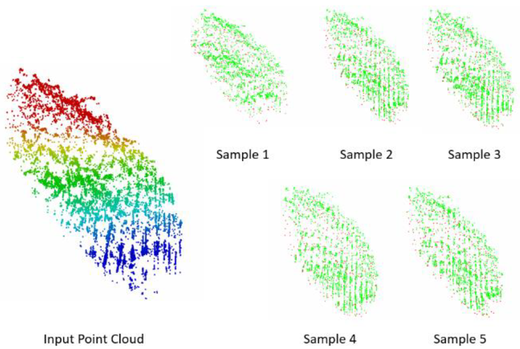
To solve the large-scale terrain expression and spatial context information of point clouds, we propose a terrain-based sampling method for DEM extraction of ALS point clouds, named T-Sampling. First, we grid the input point cloud and consider the lowest point in each grid as the base point. Second, in each grid, we randomly sample a point, except the base points, and the randomly sampled points are combined with the base points as a piece. The second step is repeated until all remaining points are combined with the base points. Figure 2 shows the results of the T-Sampling algorithm.
The advantages of the T-Sampling algorithm are as follows:
- (1)
- There is fixed density of the input point cloud. We ensure the uniformity of the point distribution in a certain range by gridding, and ensure the consistency of density by fixing the number of input points.
- (2)
- Each piece has sufficient ground points to obtain a topographic representation of the area.
2.3. Local Feature Extraction
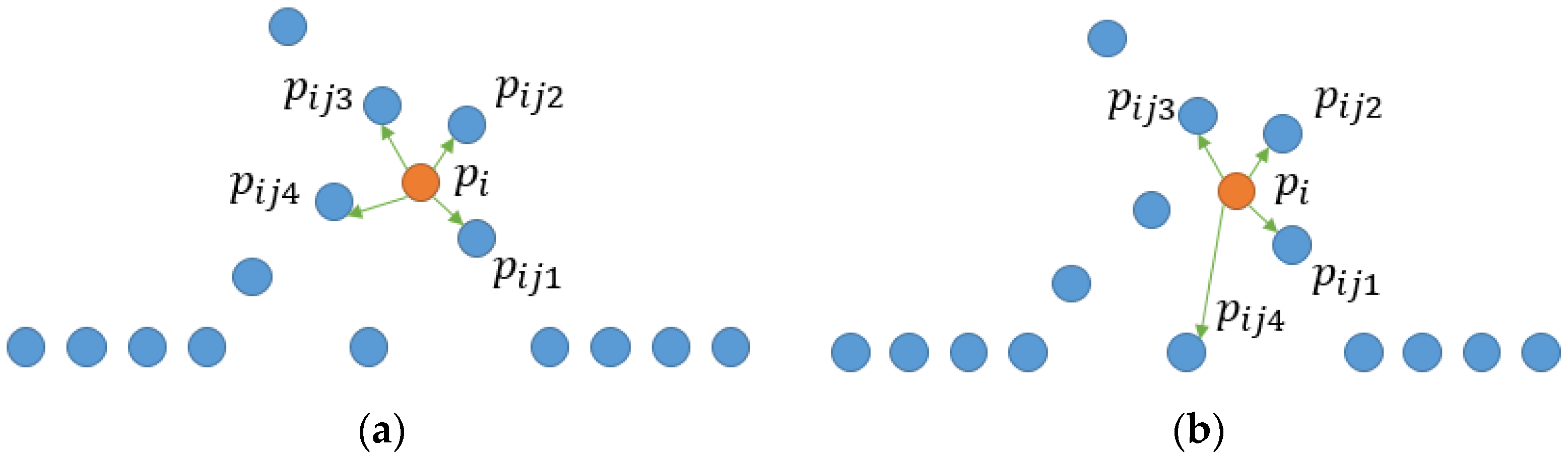
To extract the local features of ground and non-ground points in our task accurately, a Tin-EdgeConv layer is proposed to calculate the spatial features of the two kinds of points. The classical EdgeConv layer only considers the local features of the point set in the K neighborhood around a particular point. However, during the filtering task, the traditional k-nearest neighbors (KNN) method cannot describe the spatial relationship between ground and non-ground points.
Given a set of point clouds , where , we construct a graph for each point to express its relationship with other points. Specifically, we select KNN only in the x,y-direction to construct graph for each point. This graph is defined as follows:
where is the KNN of . Figure 3 illustrates the difference between the EdgeConv and Tin-EdgeConv in the graph construction stage.
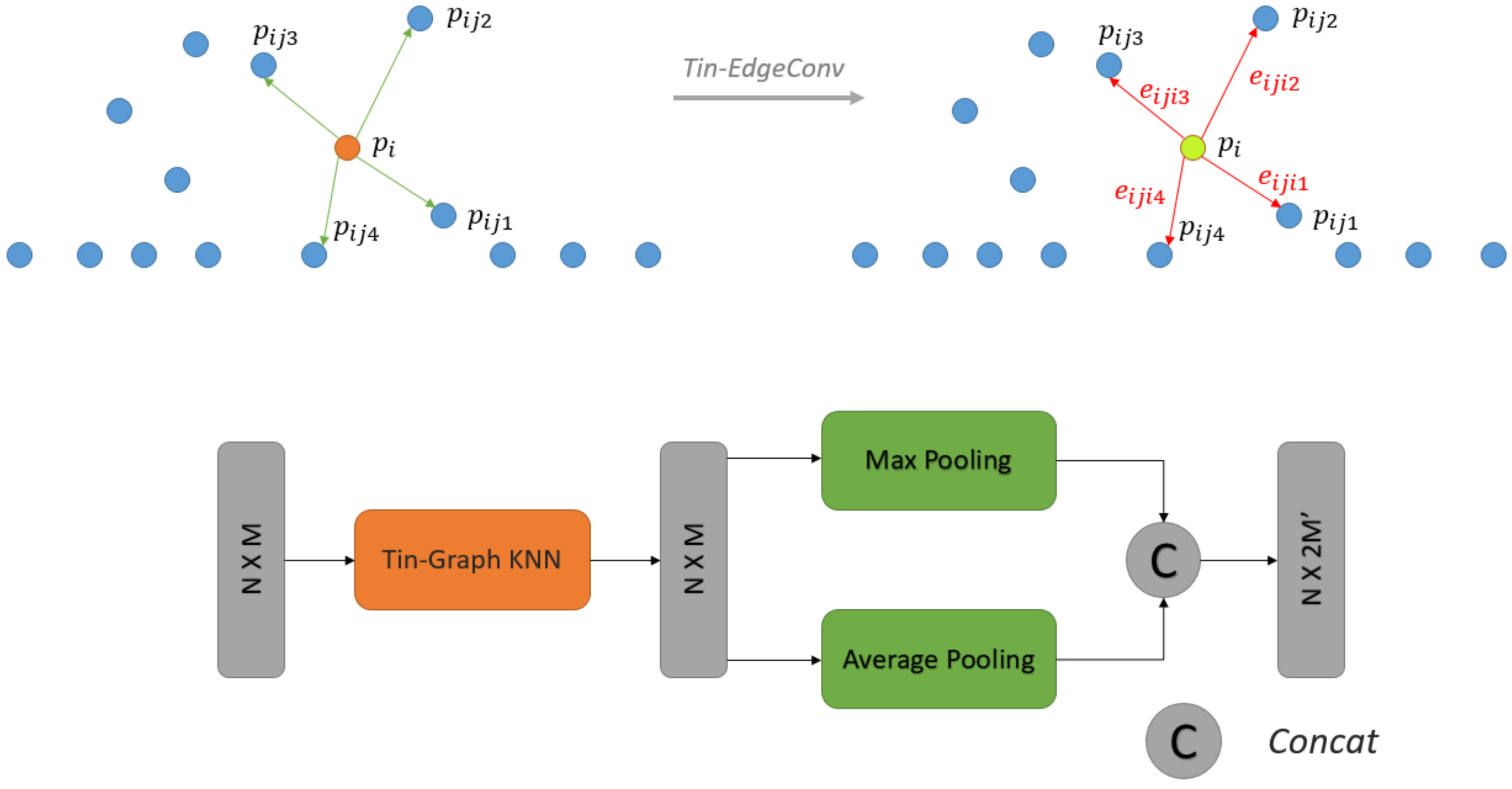
In Tin-EdgeConv, we use a directed graph, , to describe the structure of the point cloud, where and are the vertices and edges, respectively. For each point, we use the Tin-KNN graph to construct , and are the nearest points to in . The edge features are defined as , where is a nonlinear function that contains many learnable parameters, . Tin-EdgeConv initially gathers the KNNs for each point and then extracts the local edge features of points through convolution and pooling, which are useful for extracting local features. In pooling, we use the max and average pooling and concatenate their results as the output of the Tin-EdgeConv. Figure 4 presents the details of Tin-EdgeConv.
2.4. Global Feature Extraction
Global context is important for classifying cloud points and can be represented by the global features extracted using deep neural networks. However, we employ another way to extract the global features.
In this part, we use PointNet as the basic model. The principle of PointNet is that the transformation matrix can be adjusted in accordance with the final loss. PointNet ignores the transformation that will be performed eventually provided that this transformation is beneficial to the final result. PointNet uses spatial transformer network (STN) twice. The first input transform is to adjust the point cloud in the space. Intuitively, rotating an angle, such as turning an object to the front, is conducive to classification or segmentation. The second feature transform is to convert the features into high semantic information of a scene. After conducting the feature extraction for each point in the network, the global feature can be extracted for the entire point cloud using the pooling layer. These features can be combined with the local features extracted using Tin-EdgeConv in the attention model.
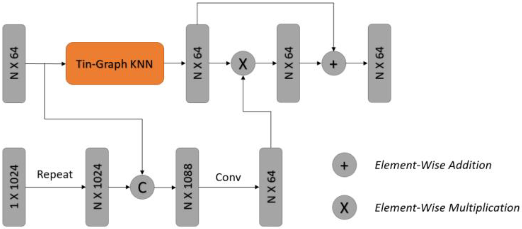
2.5. Feature Fusion Module
Existing feature fusion methods typically connect the features provided by different levels. These methods can change the dimension of connected features but cannot optimize the expression of local features through global features. To truly integrate global features into local features, we use the attention fusion module proposed by You [39] to detect the area of interest in the input point cloud.
The module consists of the fusion mask and convention parts. Given point cloud features with shape , where is the number of points, and is the dimension of features, we use Tin-EdgeConv in the convention part to compute the features , where is the input tensor of the point cloud features. The global features generated by PointNet with shape are repeated times and then concatenated with . Then, the local and global features are fused together as a relationship descriptor, which is defined as :
After the relationship descriptor, the output can be normalized to range (0, 1), generating a soft attention mask , which can be defined as:
The soft attention mask with a range of (0, 1) can describe the significance of different local structures. The final output of the block is defined as:
Figure 5 presents the details of the attention fusion module.
2.6. Inplement Details
In the T-Sampling algorithm, 4096 points per piece are selected to build the datasets. Each piece covers an area of 40 m × 40 m. During the local feature extraction stage, the output of Tin-EdgeConv is composed of a shared multilayer perceptron (MLP) network (with layer output sizes of 64, 64, 64) on each point. The architecture of the global feature extraction part is the classic PointNet with output of 1024 after max pooling operation.
The final classification result of the input points is averaged by the probability of prediction of each sliced piece, and the label of each point can be defined as:
where is the number of calculations in the sample stage, and represents the probability matrix of each calculation.
3. Experiments and Analysis
Three measurements, type I, type II, and total errors, are selected to evaluate the accuracy and correctness of the proposed method on the quantitative DEM extraction of ALS point clouds. Type I error describes the rejection of bare-earth points. Type II error is the acceptance of object points as bare earth, and the total error reflects the proportion of ground and non-ground points that are misclassified. To make the representation clearer, we define type I, type II, and total errors as , , and , respectively. The three measurements are calculated on points and defined as follows:
where a, b, c, and d represent, respectively, the number of ground points that are correctly classified, the number of ground points misclassified as non-ground points, the number of non-ground points misclassified as ground points, and the number of non-ground points correctly classified.
3.1. Experimental Dataset
To illustrate the capability of our presented framework on the DEM extraction of ALS point clouds, we evaluated it on three datasets qualitatively and quantitatively. We selected a dataset with very steep terrain in a mountainous area (dataset I), a forest dataset with terrain (dataset II), and a forest dataset with different densities (dataset III).
The point clouds published in dataset I were collected as part of a National Center for Airborne Laser Mapping (NCALM) seed grant to Alexander Neely at Penn State University. Approximately 63 km2 of data were collected in June 2018 in the Guadalupe Mountains in New Mexico and Texas. This project was designed to quantify the rock strength controls on the landscape morphology within the mountains.
The published dataset II, near Parkfield, California, was collected as an NCALM seed grant to Michael Vadman at Virginia Tech University. This dataset provides an opportunity to create a time series of spatially dense displacement measurements across the creeping/transitional portion of the San Andreas Fault from 1929 to the present. The targeted portion of the fault has experienced fairly regular M5–6 earthquakes since the approximately M7.9 Fort Tejon earthquake in 1857, which ruptured from Parkfield to San Bernardino.
The point clouds in dataset III were collected in South China. Each point cloud has an area of 500 m × 500 m, with an average density of 0.5–35 points/. All the evaluating ground truths were produced through the DEM production process, including automatic filtering by TerraScan software and post-manual editing.
The details of the three datasets are summarized in Table 1.
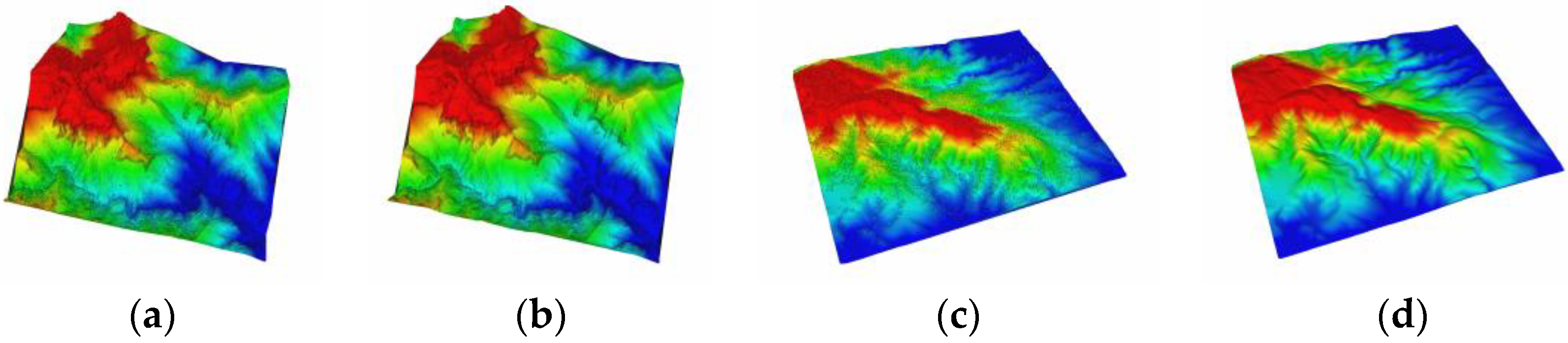
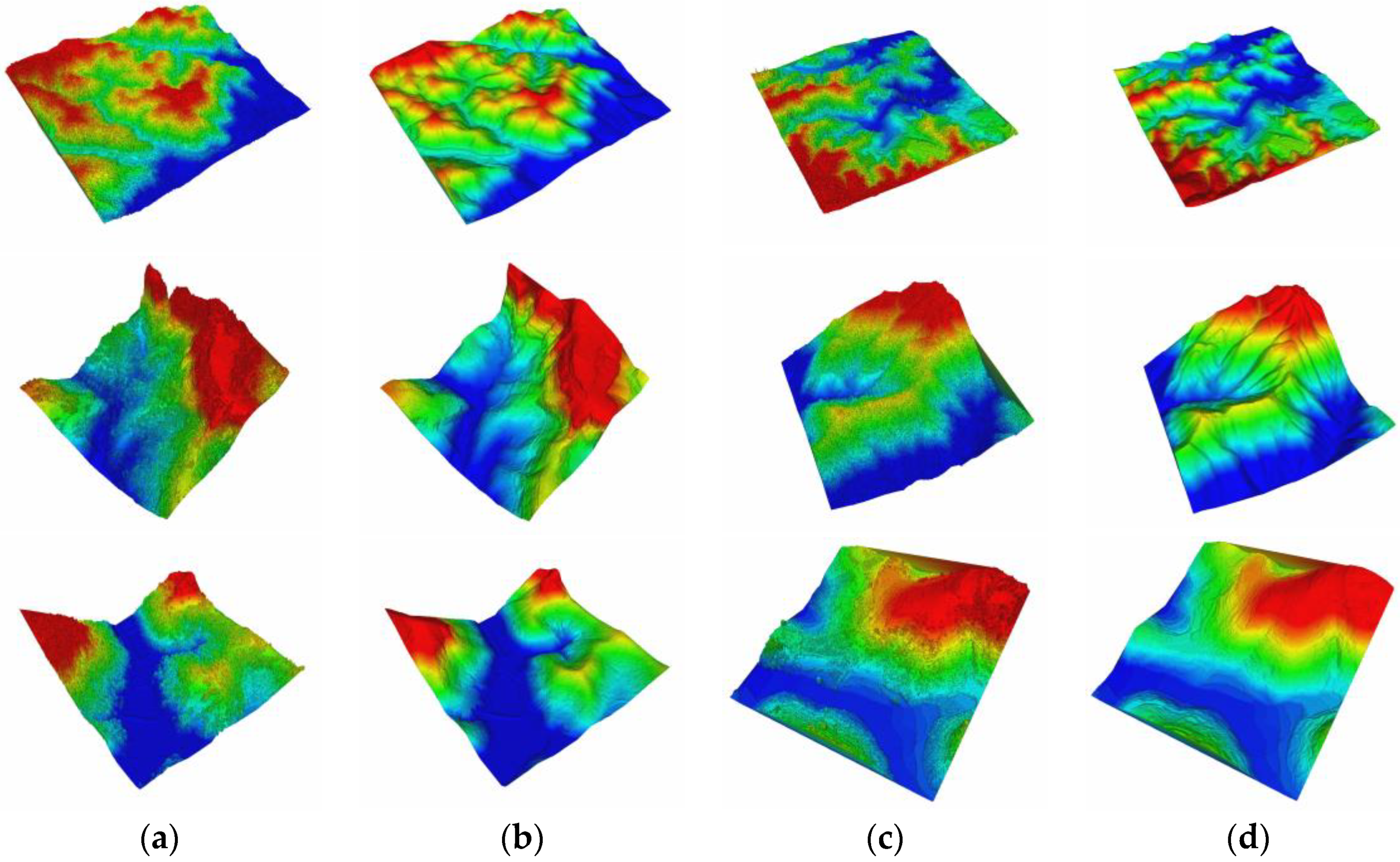
The experimental data were colored in accordance with the elevation rendering of a digital surface model (DSM), and the results of manual extraction of the DEM are demonstrated in Figure 6 and Figure 7. The cross-sections of some data are shown in Figure 8. The three datasets have different characteristics: dataset I is mainly dominated by steep ridges, dataset II is mainly composed of gentle forest areas, and dataset III is complex and diverse.
3.2. Comparative Analysis and Accuracy Evaluation of DEM Extraction
To prove the effectiveness of the proposed method, the experimental results were compared with handcrafted- and deep learning-based methods. In the handcrafted-based methods, the progressive triangulation-based method in TerraSolid and the cloth simulation filter (CSF)-based method in CloudCompare were compared with the proposed framework. In the deep learning-based methods, we compared the methods in two stages, namely, the data preprocessing and network inference stages. During data preparation, we compared our Tin-Sampling method with the random sampling method in PointCNN in our proposed network. During the network inference stage, we compared our proposed network with the dynamic graph convolutional neural network (DGCNN)-segmentation network and DCNN network in accordance with our proposed data preparation method. In addition, SparseConvNet [40], as the voxel-based point cloud processing network, was compared to prove the effectiveness of the proposed framework.
3.2.1. Experimental Results Compared with Handcrafted-Based Methods.
In this section, we compare our proposed framework with two classic software programs, TerraSolid and CloudCompare, on published datasets I and II. Various combinations of parameters for TerraSolid and CSF were selected, and the optimal results are chosen. The accuracies of the different methods are shown in Table 2.
As shown in Table 2, the proposed method is superior to the handcrafted-based methods. The algorithm in TerraSolid gets the lowest but the highest , indicating that it has insufficient ability to extract ground points in forest areas. The algorithm needs to select the iterative distance and angle of the triangular face in the processing. However, in forest area, the terrain undulates, and excessive iteration distances and angles will mistake vegetation points such as trees as ground points.
Compared with TerraSolid, the CSF in CloudCompare has better terrain retention capability. However, CSF uses cloth to simulate the terrain, so the performance on low vegetation is poor, resulting in a relatively coarse DEM. These two traditional methods are flawed in design and cannot adapt to complex forest scenes, so the of extraction results was relatively high. The proposed framework is based on deep learning. Feature extraction was performed by deep convolution neural network, which guaranteed the robustness of the extracted features and balanced the terrain preservation and surface smoothness. Therefore, the framework proposed in this paper achieved a minimum of 17.27% and 8.74% on datasets I and II, respectively. Figure 9 shows the details of terrain extraction on dataset I.
3.2.2. Experimental Results of Data Preprocessing Algorithm
The random sampling method proposed by PointCNN, R-Sampling, was compared with our proposed T-Sampling method. The inferred network for these methods is the proposed network. We compared the effects of the two sampling methods on the extraction results on public datasets I and II. The accuracies of the different methods are shown in Table 3, and a detailed comparison is illustrated in Figure 10.
As seen in Table 3, the proposed T-Sampling method is superior to the R-Sampling method. For an input point cloud, the points sampled by R-Sampling method are random, that is, the ratio of the sampled ground and non-ground points may have extreme deviation. In a sampled point cloud, it is very likely that only a few ground points are sampled, and these ground points cannot describe the trend of the terrain. Due to the uncertainty of data distribution after sampling, the network cannot accurately predict the label of points, causing a lot of random noise, shown in Figure 10a, and too many ground points are lost. However, in the proposed T-Sampling method, each sampling contains most of the ground points, which can guarantee capturing the fluctuations of terrain. Meanwhile, the DEM results predicted by the network are smoother and without random noise. Therefore, the T-Sampling method proposed in this paper can significantly improve the results of DEM extraction.
3.2.3. Experimental Results during Network Inference Stage
DGCNN, SparseConvNet, and DCNN [27] were compared with our proposed Tin-EdgeConv and attention fusion block. We evaluated it on the two public datasets, I and II. The accuracies of the different networks are presented in Table 4.
It can be seen from Table 4 that the proposed method gets the lowest on the two public datasets, indicating that it works best. The DCNN method converts each point to an RGB image in accordance the differences in elevation. However, in a forest area, the converted image cannot express the differences between ground and non-ground points because of the steep terrain and sparse ground points. In addition, there is a loss of information in the process of transforming from 3D point cloud to 2D image. In a complex forest area, such information loss will cause serious misclassification. SparseConvNet converts point clouds into voxels and applies sparse convolution to extract the features. In the process of voxelization, due to the limited voxel resolution, there may be multiple points in one voxel. Therefore, it is difficult to separate vegetation points close to the ground surface. This caused the method to have a relatively high . Compared with DGCNN, our proposed Tin-EdgeConv layer can express the relationship between ground and non-ground points better. Meanwhile, the attention fusion module fused the extracted local features and global context information better than the concatenate operation in DGCNN.
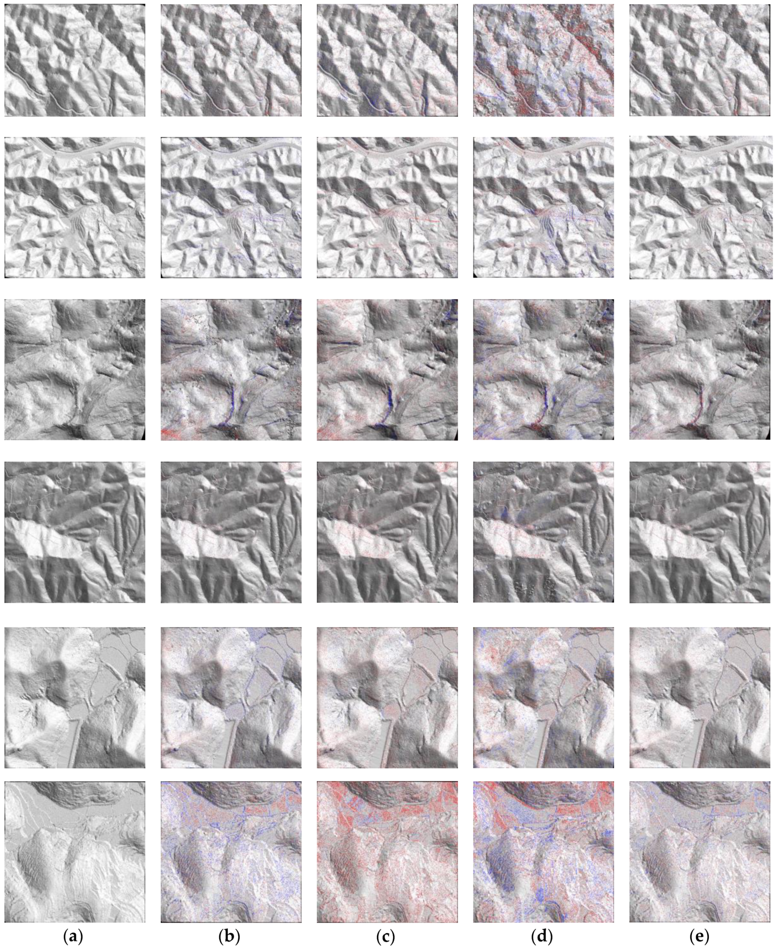
To verify the scalability of the proposed method, we validated it by using dataset III, and the accuracies are shown in Figure 11.
From Figure 11, it can be seen our proposed method gets the lowest on dataset III, indicating that it has a strong generalization ability. The filtered details are shown in Figure 12.
Figure 12e shows the least red and blue points, which means the proposed network has the highest classification accuracy.
3.2.4. Efficiency Analysis
Although the proposed method has higher accuracy than previous methods, it also has shortcomings. Influenced by the complexity of deep neural networks, the proposed method is relatively inefficient. We evaluated the efficiency of some algorithms on dataset III, and the statistical results are shown in Table 5.
The proposed method has significantly lower efficiency than TerraSolid. The proposed T-Sampling method and the Tin-EdgeConv module have high computational cost in data preprocessing and network inference, repectively. Therefore, how to improve the calculation efficiency will be the next step for us to improve the algorithm.
4. Discussion
4.1. Main Goals of the Study
The main goals of this study were to classify ground and non-ground points to extract DEM using ALS point cloud data. By performing the proposed terrain-based random sampling, T-Sampling, on the point cloud, the data of the input network are more differentiated. The feature representation is enhanced by an attention fusion module which fuses global context features and local features extracted by PointNet and the proposed Tin-EdgeConv, respectively. Finally, the proposed method gets better classification accuracy.
4.2. Steep Slopes
Complex steep slopes often occur in forest areas. The difficulty of processing this kind of area is mainly in retaining the necessary topographic feature points to avoid the loss of key points. However, handcrafted algorithms are limited by designed parameters and cannot process other types of terrain with the same parameters while dealing with steep slopes. For example, in the CSF algorithm, many parameters need to be designed, including grid resolution, which represents the horizontal distance between two neighboring particles, and rigidness, which controls the rigidness of the cloth. These parameters are determined by a number of tests. In large-scale ALS point cloud data, there will be many types of terrain. For different terrain, different parameters need to be designed, which makes DEM extraction more difficult.
The proposed method in this paper avoids the chosen parameter and directly processes the point cloud in an end-to-end manner. It automatically adapts to different types of terrains through the parameter learning of the network. A typical extracted DEM is shown in Figure 13.
4.3. Compared with Handcrafted-Based Algorithms
Handcrafted-based algorithms are mostly based on artificially designed features, which are only used to process the specific terrain and are not robust. In complex forest areas, multiple terrains often exist, such as steep slopes and gentle woodlands. For different terrains, different parameters need to be chosen, which requires identifying the scene category before applying handcrafted algorithms for DEM extraction.
The algorithm in TerraSolid is based on progressive triangulation. It first grids the processed area and takes the lowest point of each grid as the seed point. Then, a triangular network is constructed by the initial seed points. Finally, points are added to the triangular network if it is below threshold values. In the implementation of this algorithm, there are two core problems that need to be solved. First, the size of the grid needs to be determined to choose initial seed points. If the ground points are sparse, vegetation points will be selected to be the seed points if a small grid size is set. The initialized seed points are selected within a user-defined grid. The size of the grid is usually based on the largest type of structure. Second, the parameters for triangular network densification, such as distance to the TIN facets and angles to the nodes, are derived from processed data. A point to be calculated in each TIN facet is added if it meets the criteria based on the designed threshold parameters. As shown in Figure 14, the parameters of distance to facet planes and angles to nodes , and , are the core values. However, the setting of these parameters is very strict. So how to choose the appropriate parameters more reasonably is the biggest difficulty of this method.
However, the proposed method is based on deep learning framework, which does not need to set any parameters. The proposed network can be regarded as a composite function composed of many simple functions, which can implement very complex transformations. It can automatically extract progressively high-level features from the original data, and such high-level features are often more universal than designed features.
4.4. Compared with Existing Network
DCNN [27] is the first method to apply deep learning to point cloud DEM extraction. The method transforms each point into an image according to the neighboring points within a window. Therefore, the task can be considered as the classification of an image. It achieves very good results on simple terrain. However, in forest areas, the process of transforming points into images can cause serious information loss. In steep areas, there are usually huge fluctuations. If such huge fluctuations are converted into an image in the range of 0–255, the terrain information will be compressed.
SparseConvNet [40] is a representative point cloud processing method for large scenes. The method is based on the traditional 3D convolutional neural network. By adding sparse representation and sparse convolution kernel, it guarantees accuracy while reducing running time and GPU memory occupation. SparseConvNet can adopt 2D convolutional network frameworks in image processing, such as U-Net and ResNet architecture. However, for a 3D convolutional network, it is difficult to set appropriate voxel resolution. The distribution of a point cloud obtained by ALS is very irregular, which makes it impossible to set a suitable resolution to ensure that there is only one point in each voxel. Although the sparse convolutional framework can reduce the memory usage, it will still cause memory overflow if the voxel resolution is set too small.
PointNet [31] is a pioneering effort that directly processes point clouds. The basic idea of PointNet is to learn a spatial encoding of each point, and then aggregate all the point features. It greatly improves the effect of point cloud processing. However, PointNet encodes each point individually, without considering its spatial context information. The final high-level features obtained by the max pooling operation is the global information of the entire point cloud.
DGCNN [36] is the first network to use graph convolutional neural networks to process point clouds. It contains the core module, EdgeConv, which considers the spatial context by adding neighboring information with the KNN algorithm. However, for ALS point cloud data, the traditional KNN algorithm cannot guarantee the spatial position relationship between ground and non-ground points.
Inspired by the EdgeConv module, the proposed Tin-EdgeConv module can solve this problem. When constructing a directed graph, Tin-EdgeConv only finds neighboring points in the x,y-axis. Therefore, the constructed directed graph can contain the spatial context information of selected points in the z-axis. After obtaining the local features through Tin-EdgeConv, we extract the global features by PointNet. These two modules are independent of each other. To fully combine the two features, the attention fusion module is employed instead of a concatenate operation. The traditional feature fusion operation, concat, just increases the dimension of the final feature and cannot fuse the two features together, and the final merged features are still independent of each other. However, the attention fusion module employed in this paper converts the global features into an attention matrix. By learning the matrix in the network, the optimized matrix is multiplied with the extracted local features to optimize the results of local feature extraction. All of the proposed modules consider the particularities of ALS point clouds.
5. Conclusions
This study presents a DEM extraction framework for ALS point clouds for the data preparation and network inference stages. The T-Sampling algorithm is proposed to split the source data into several pieces. Each piece consists of sufficient points to express the terrain information. Then, each piece of the point cloud is computed using two feature extraction stages, local feature extraction based on the proposed Tin-EdgeConv layers and the global feature extraction based on PointNet. The outputs of the two feature extractions are fused by the attention block, which enhances the expression of the relationship of points. In comparison with the results from other DEM extraction methods and the baseline of DGCNN, as well as TerraSolid and CSF, the extraction accuracy using the proposed framework can satisfy practical applications. The proposed framework is efficient and valid for DEM extraction. In addition, the proposed method can provide a convenient and effective way to extract DEM in forest areas of ALS point clouds.
For future works, we will focus the following areas: a new deep-learning-based framework for DEM extraction in urban areas, and a new method to promote the performance of the proposed method and improve work efficiency.
Author Contributions
J.Z. conceived and designed the algorithms and experiments, and wrote the manuscript; X.H. guided the algorithm design and revised the manuscript; H.D. provided a part of the comparative experimental results; S.Q. provided experimental environment. All authors have read and agreed to the published version of the manuscript.
Funding
This research was funded by the National Key Research and Development Program of China, grant number 2016YFF0103503; the research funding from Guangzhou City (201604010123) of China.
Acknowledgments
The authors thank Guangzhou Jiantong Surveying, Mapping, and Geographic Information Technology Ltd. for providing the data used in this research project.
Conflicts of Interest
The authors declare no conflict of interest.
References
- Kada, M. 3D building generalization based on half-space modeling. Int. Arch. Photogramm. Remote Sens. Spat. Inf. Sci. 2006, 36, 58–64. [Google Scholar]
- Axelsson, P. DEM generation from laser scanner data using adaptive TIN models. Proc. Int. Arch. Photogramm. Remote Sens. 2000, 33, 110–117. [Google Scholar]
- Vosselman, G. Slope based filtering of laser altimetry data. Int. Arch. Photogramm. Remote Sens. Spat. Inf. Sci. 2000, 33, 935–942. [Google Scholar]
- Sithole, G.; Vosselman, G. Experimental comparison of filter algorithms for bare-Earth extraction from airborne laser scanning point clouds. ISPRS J. Photogramm. Remote Sens. 2004, 59, 85–101. [Google Scholar] [CrossRef]
- Kraus, K.; Pfeifer, N. Determination of terrain models in wooded areas with airborne laser scanner data. ISPRS J. Photogramm. Remote Sens. 1998, 53, 193–203. [Google Scholar] [CrossRef]
- Kami’nski, W. M-Estimation in the ALS cloud point filtration used for DTM creation. In GIS for Geoscientists; Hrvatski Informatiˇcki Zbor-GIS Forum: Zagreb, Croatia; University of Silesia: Katowice, Poland, 2012; p. 50. [Google Scholar]
- Błaszczak-Bak, W.; Janowski, A.; Kami’nski, W.; Rapi’nski, J. Application of the Msplit method for filtering airborne laser scanning datasets to estimate digital terrain models. Int. J. Remote Sens. 2015, 36, 2421–2437. [Google Scholar] [CrossRef]
- Błaszczak-Bak, W.; Janowski, A.; Kami’nski, W.; Rapi’nski, J. ALS data filtration with fuzzy logic. J. Indian Soc. Remote Sens. 2011, 39, 591–597. [Google Scholar]
- Lindenberger, J. Laser-Profilmessungen zur Topographischen Gelandeaufnahme. Ph.D. Thesis, Stuttgart University, Stuttgart, Germany, 1992. [Google Scholar]
- Hu, X.; Ye, L.; Pang, S.; Shan, J. Semi-global filtering of airborne LiDAR data for fast extraction of digital terrain models. Remote Sens. 2015, 7, 10996–11015. [Google Scholar] [CrossRef]
- Bigdeli, B.; Amirkolaee, H.A.; Pahlavani, P. DTM extraction under forest canopy using LiDAR data and a modified invasive weed optimization algorithm. Remote Sens. Environ. 2018, 216, 289–300. [Google Scholar] [CrossRef]
- Hsu, C.W.; Lin, C.J. A comparison of methods for multiclass support vector machines. IEEE Trans. Neural Netw. Learn. 2002, 13, 415–425. [Google Scholar]
- Cutler, A.; Cutler, D.R.; Stevens, J.R. Random forests. Mach. Learn. 2011, 45, 157–176. [Google Scholar]
- Zhu, J.; Arbor, A.; Hastie, T. Multi-class AdaBoost. Stat. Interface 2006, 2, 349–360. [Google Scholar]
- Chehata, N.; Guo, L.; Mallet, C. Contribution of airborne full-waveform lidar and image data for urban scene classification. In Proceedings of the IEEE International Conference on Image Processing (ICIP), Cairo, Egypt, 7–10 November 2009; pp. 1669–1672. [Google Scholar]
- Mallet, C.; Bretar, F.; Roux, M.; Soergel, U.; Heipke, C. Relevance assessment of full-waveform lidar data for urban area classification. ISPRS J. Photogramm. Remote Sens. 2011, 66, S71–S84. [Google Scholar] [CrossRef]
- Kim, H.B.; Sohn, G. Random forests based multiple classifier system for power-line scene classification. Int. Arch. Photogramm. Remote Sens. Spat. Inf. Sci. 2011, XXXVIII, 253–258. [Google Scholar] [CrossRef] [Green Version]
- Kang, Z.; Yang, J.; Zhong, R. A bayesian-network-based classification method integrating airborne lidar data with optical images. IEEE JSTARS 2017, 10, 1651–1661. [Google Scholar] [CrossRef]
- Zhang, Z.; Zhang, L.; Tong, X.; Guo, B.; Zhang, L.; Xing, X. Discriminative-dictionary-learning-based multilevel pointcluster features for ALS point-cloud classification. IEEE Trans. Geosci. Remote 2016, 54, 7309–7322. [Google Scholar] [CrossRef]
- Munoz, D.; Bagnell, J.A.; Vandapel, N.; Hebert, M. Contextual classification with functional max-margin markov networks. In Proceedings of the IEEE Conference on Computer Vision and Pattern Recognition (CVPR), Miami Beach, FL, USA, 20–25 June 2009; pp. 975–982. [Google Scholar]
- Munoz, D.; Vandapel, N.; Hebert, M. Directional associative markov network for 3-D point cloud classification. In Proceedings of the 4th International Symposium on 3D Data Processing, Visualization and Transmission, Atlanta, GA, USA, 18–20 June 2008; pp. 65–72. [Google Scholar]
- Najafi, M.; Namin, S.T.; Salzmann, M.; Petersson, L. Non-associative higher-order markov networks for point cloud classification. In Proceedings of the European Conference on Computer Vision (ECCV), Zurich, Switzerland, 6–12 September 2014; Springer: Cham, Switzerland, 2014; pp. 500–515. [Google Scholar]
- Kumar, S.; Hebert, M. Discriminative random fields. Int. J. Comput. Vis. 2006, 68, 179–201. [Google Scholar] [CrossRef] [Green Version]
- Niemeyer, J.; Rottensteiner, F.; Soergel, U. Classification of urban LiDAR data using conditional random field and random forests. In Proceedings of the IEEE Urban Remote Sensing Event (JURSE), Sao Paulo, Brazil, 21–23 April 2013; pp. 139–142. [Google Scholar]
- Schmidt, A.; Niemeyer, J.; Rottensteiner, F.; Soergel, U. Contextual classification of full waveform lidar data in the Wadden Sea. IEEE Geosci. Remote Soc. 2014, 11, 1614–1618. [Google Scholar] [CrossRef]
- Niemeyer, J.; Rottensteiner, F.; Soergel, U. Contextual classification of lidar data and building object detection in urban areas. ISPRS J. Photogramm. Remote Sens. 2014, 87, 152–165. [Google Scholar] [CrossRef]
- Xiangyun, H.; Yi, Y. Deep-learning-based classification for DTM extraction from ALS point cloud. Remote Sens. 2016, 8, 730. [Google Scholar]
- Su, H.; Maji, S.; Kalogerakis, E.; Learned-Miler, E. Multi-view convolutional neural networks for 3D shape recognition. In Proceedings of the IEEE International Conference on Computer Vision (ICCV), Santiago, Chile, 13–18 December 2015; pp. 945–953. [Google Scholar]
- Maturana, D.; Scherer, S. Voxnet: A 3d convolutional neural network for real-time object recognition. In Proceedings of the IEEE/RSJ International Conference on Intelligent Robots and Systems (IROS), Hamburg, Germany, 28 September–2 October 2015; pp. 922–928. [Google Scholar]
- Zhou, Y.; Tuzel, O. Voxelnet: End-to-end learning for point cloud based 3d object detection. In Proceedings of the IEEE Conference on Computer Vision and Pattern Recognition (CVPR), Salt Lake City, UT, USA, 18–22 June 2018; pp. 4490–4499. [Google Scholar]
- Qi, C.R.; Yi, L.; Su, H.; Guibas, L.J. Pointnet: Deep learning on point sets for 3d classification and segmentation. In Proceedings of the IEEE Conference on Computer Vision and Pattern Recognition (CVPR), Honolulu, HI, USA, 21–26 July 2017; pp. 652–660. [Google Scholar]
- Qi, C.R.; Yi, L.; Su, H.; Guibas, L.J. Pointnet++: Deep hierarchical feature learning on point sets in a metric space. In Proceedings of the Conference on Neural Information Processing Systems (NIPS), Long Beach, CA, USA, 4–9 December 2017; pp. 5099–5108. [Google Scholar]
- Li, Y.; Bu, R.; Sun, M.; Wu, W.; Di, X.; Chen, B. Pointcnn: Convolution on x-transformed points. In Proceedings of the Neural Information Processing Systems (NIPS), Montreal, QC, Canada, 3–8 December 2018; pp. 820–830. [Google Scholar]
- Rethage, D.; Wald, J.; Sturm, J.; Navab, N.; Tombari, F. Fully-convolutional point networks for large-scale point clouds. In Proceedings of the European Conference on Computer Vision (ECCV), Munich, Germany, 8–14 September 2018; pp. 596–611. [Google Scholar]
- Jiang, M.; Wu, Y.; Zhao, T.; Zhao, Z.; Lu, C. Pointsift: A sift-like network module for 3D point cloud semantic segmentation. arXiv 2018, arXiv:1807.00652. [Google Scholar]
- Wang, Y.; Sun, Y.; Liu, Z.; Sarma, S.E.; Bronstein, M.M.; Solomon, J.M. Dynamic graph cnn for learning on point clouds. ACM Trans. Graphics (TOG) 2019, 38, 146. [Google Scholar] [CrossRef] [Green Version]
- Te, G.; Hu, W.; Guo, Z.; Zheng, A. Rgcnn: Regularized graph cnn for point cloud segmentation. In Proceedings of the ACM Multimedia Conference on Multimedia Conference, Seoul, Korea, 22–26 October 2018; pp. 746–754. [Google Scholar]
- Landrieu, L.; Simonovsky, M. Large-scale point cloud semantic segmentation with superpoint graphs. In Proceedings of the IEEE Conference on Computer Vision and Pattern Recognition (CVPR), Salt Lake City, UT, USA, 18–22 June 2018; pp. 4558–4567. [Google Scholar]
- You, H.; Feng, Y.; Ji, R.; Yue, G. Pvnet: A joint convolutional network of point cloud and multi-view for 3D shape recognition. In Proceedings of the ACM Multimedia Conference on Multimedia Conference, Seoul, Korea, 22–26 October 2018; pp. 1310–1318. [Google Scholar]
- Graham, B.; Engelcke, M.; Van Der Maaten, L. 3D semantic segmentation with submanifold sparse convolutional networks. In Proceedings of the IEEE Conference on Computer Vision and Pattern Recognition (CVPR), Salt Lake City, UT, USA, 18–22 June 2018; pp. 9224–9232. [Google Scholar]
Figure 1.
Overview of our proposed framework for the digital elevation model (DEM) extraction of airborne laser scanning (ALS) point clouds (colors represent various categories).
Figure 1.
Overview of our proposed framework for the digital elevation model (DEM) extraction of airborne laser scanning (ALS) point clouds (colors represent various categories).

Figure 2.
Result of T-Sampling algorithm (red: base points; green: additional points).

Figure 3.
Difference between (a) classic k-nearest neighbors (KNN) and (b) Tin-KNN graphs.

Figure 4.
Top: Visualization of Tin-EdgeConv operation; bottom: Tin-EdgeConv structure.

Figure 5.
Attention fusion module.

Figure 6.
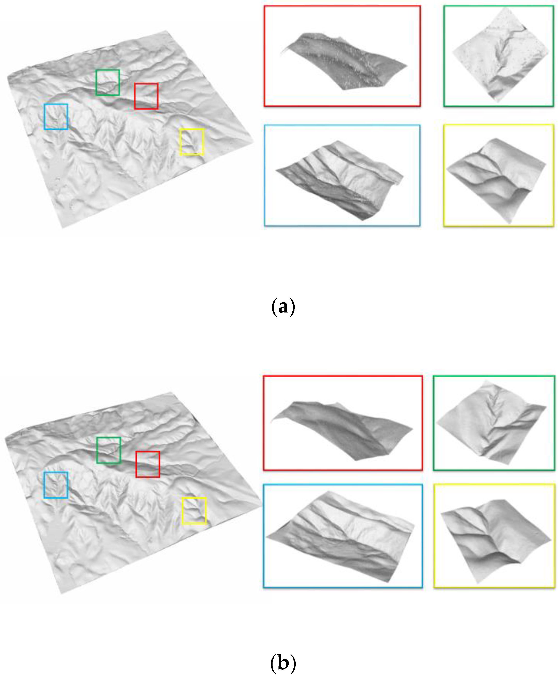
(a,b) Elevation rendering of digital surface model (DSM) and manual extraction digital elevation model (DEM), respectively, of dataset I; (c,d) elevation of DSM and manual extraction DEM, respectively, of dataset II.
Figure 6.
(a,b) Elevation rendering of digital surface model (DSM) and manual extraction digital elevation model (DEM), respectively, of dataset I; (c,d) elevation of DSM and manual extraction DEM, respectively, of dataset II.

Figure 7.
(a,c) Elevation rendering of DSM and (b,d) manual extraction DEM of dataset III.

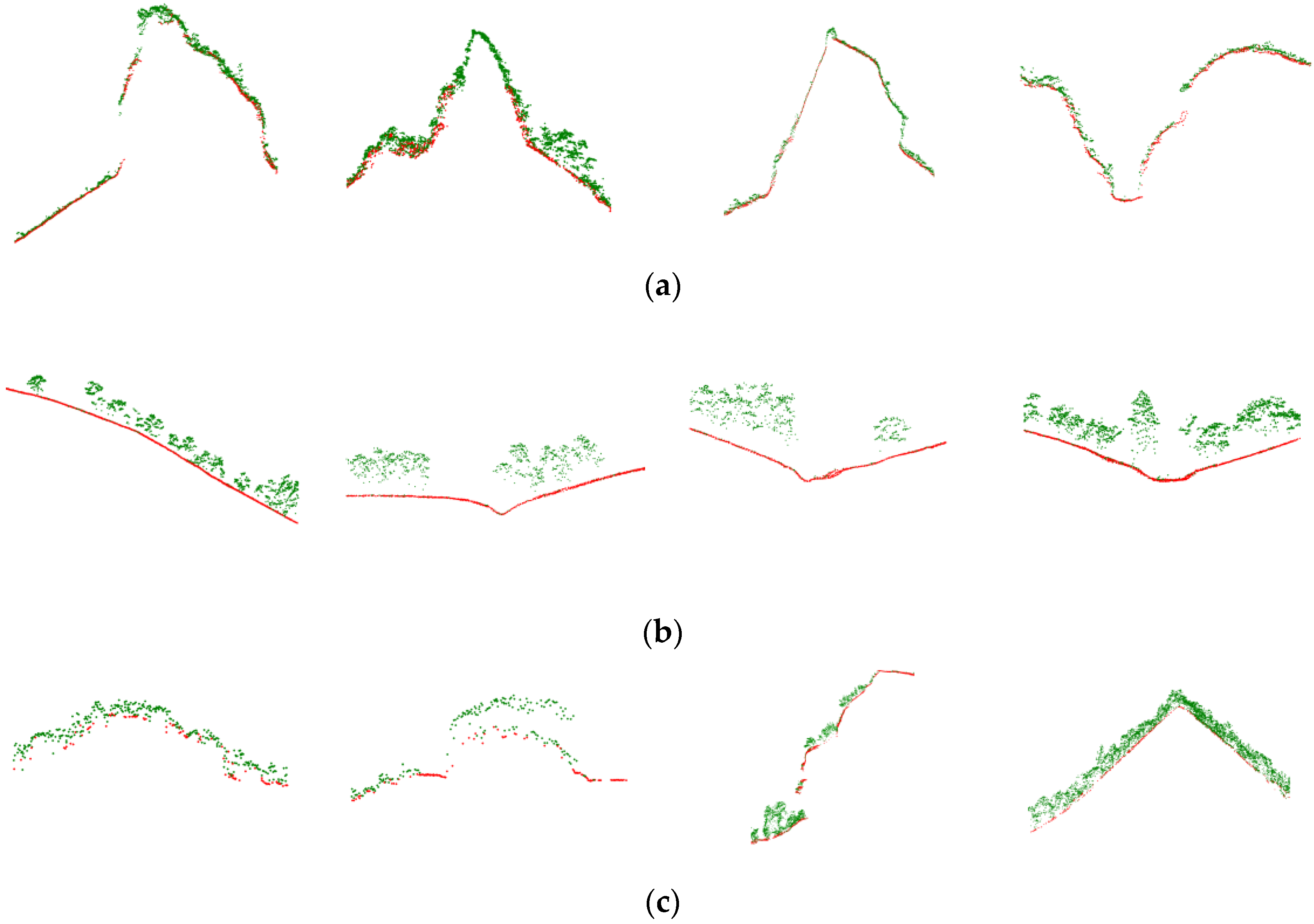
Figure 8.
(a–c) Cross-sections of datasets I, II, and III, respectively. Red and green represent manual extracted ground points and non-ground points, respectively.
Figure 8.
(a–c) Cross-sections of datasets I, II, and III, respectively. Red and green represent manual extracted ground points and non-ground points, respectively.

Figure 9.
Filtered results of dataset I: (a) TerraSolid; (b) CSF; (c) proposed framework; (d) GroundTruth.
Figure 9.
Filtered results of dataset I: (a) TerraSolid; (b) CSF; (c) proposed framework; (d) GroundTruth.

Figure 10.
Filtered results of Dataset II: (a) R-Sampling method; (b) proposed T-Sampling method.

Figure 11.
Comparison of DGCNN, SparseConvNet, DCNN, and proposed network on dataset III: (a–c) represent the type I error, type II error, and total error, respectively.
Figure 11.
Comparison of DGCNN, SparseConvNet, DCNN, and proposed network on dataset III: (a–c) represent the type I error, type II error, and total error, respectively.

Figure 12.
Comparison of proposed network with DGCNN, SparseConvNet, and DCNN regarding DEM details. (a) Ground truth triangulated irregular network (TIN)-rendered gray images of evaluated data, and TIN-rendered DEM extracted from the results of filtration by (b) DGCNN, (c) SparseConvNet, (d) DCNN, and (e) proposed network. Red denotes accepted non-ground points, blue denotes rejected ground points.

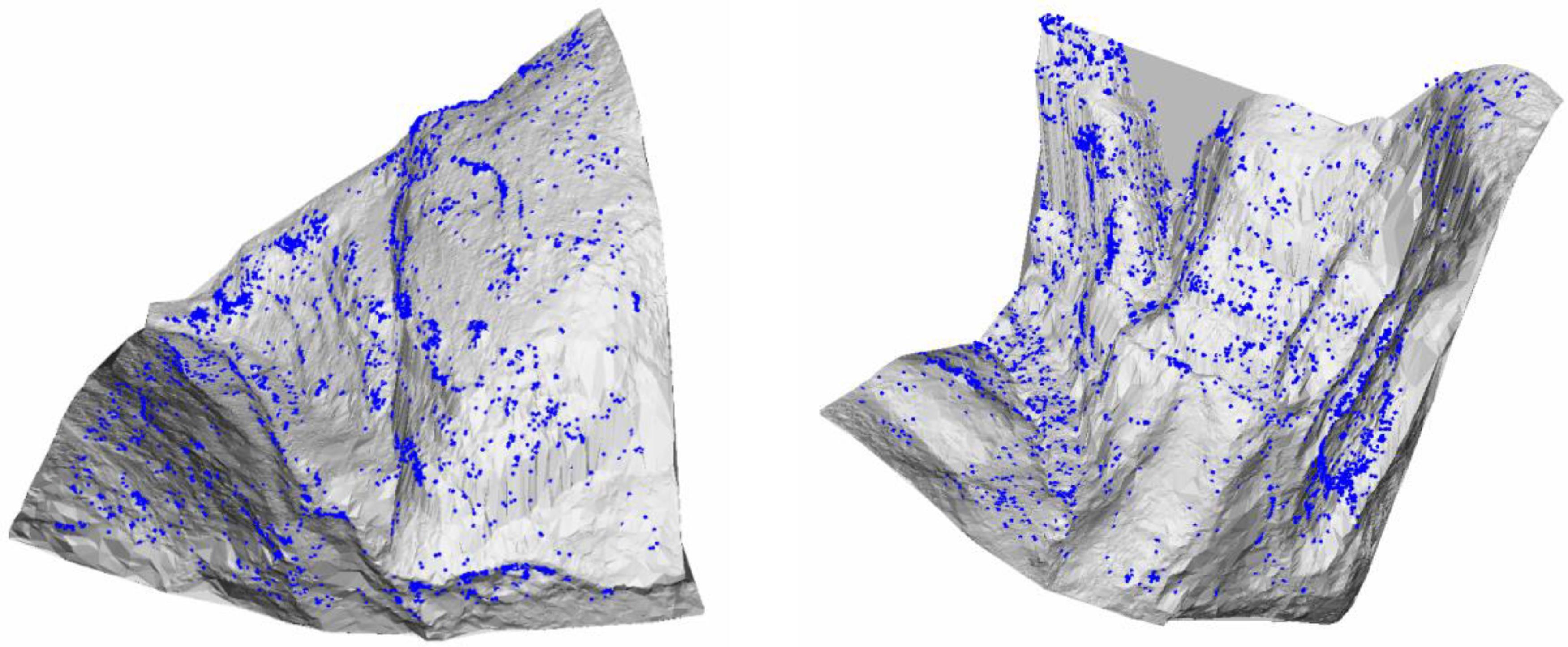
Figure 13.
Extracted DEM of area 3 in dataset III. Blue denotes rejected ground points.

Figure 14.
Calculated values for a data point during TIN densification.


Table 1.
Three datasets for our experiments.
| DataSet | Ground Points (K) | Non-Ground Points (Unit: K) | Density (Unit: points/ ) | |
|---|---|---|---|---|
| I | 14,184.2 | 24,189.6 | 18.487 | |
| II | 26,961.3 | 20,697.9 | 17.027 | |
| III | Area 1 | 79.2 | 543.5 | 0.736 |
| Area 2 | 756.1 | 2548.4 | 3.163 | |
| Area 3 | 556.4 | 1976.6 | 34.691 | |
| Area 4 | 392.9 | 2846.2 | 3.183 | |
| Area 5 | 642.9 | 1924.1 | 35.110 | |
| Area 6 | 460.7 | 789.5 | 19.614 | |
Table 2.
Comparison of accuracy with handcrafted-based methods on dataset I and II.
| Method | Dataset I | Dataset II | ||||
|---|---|---|---|---|---|---|
| TerraSolid | 86.37 | 0.09 | 31.98 | 71.31 | 0.06 | 40.37 |
| CSF | 27.83 | 41.55 | 36.48 | 1.99 | 24.82 | 11.91 |
| Proposed | 36.12 | 6.22 | 17.27 | 3.53 | 15.54 | 8.74 |
Table 3.
Comparison of R-Sampling and T-Sampling algorithm on dataset I and II.
| Method | Dataset I | Dataset II | ||||
|---|---|---|---|---|---|---|
| Proposed Network + R-Sampling | 68.66 | 28.37 | 69.17 | 11.38 | 15.48 | 13.17 |
| Proposed Network + T-Sampling | 36.12 | 6.22 | 17.27 | 3.53 | 15.53 | 8.74 |
Table 4.
Comparison of DGCNN, SparseConvNet, DCNN, and the proposed network on dataset I and II.
| Method | Dataset I | Dataset II | ||||
|---|---|---|---|---|---|---|
| DGCNN | 43.58 | 4.61 | 19.02 | 9.77 | 10.73 | 10.19 |
| SparseConvNet | 35.23 | 9.35 | 18.92 | 3.84 | 20.03 | 10.88 |
| DCNN | 42.92 | 9.47 | 21.84 | 7.76 | 18.10 | 12.27 |
| Ours | 36.12 | 6.22 | 17.27 | 3.53 | 15.54 | 8.74 |
Table 5.
Comparison of efficiency with some algorithms (seconds).
| Dataset III | Number of Points (K) | Methods | |||
|---|---|---|---|---|---|
| CSF | TerraSolid | DCNN | Ours | ||
| Area 1 | 622.7 | 463.1 | 4.3 | 1120.8 | 14.0 |
| Area 2 | 3304.5 | 224.3 | 10.1 | 5948.1 | 245.1 |
| Area 3 | 2533.0 | 163.5 | 9.2 | 4559.4 | 147.6 |
| Area 4 | 3239.1 | 337.7 | 9.7 | 5830.4 | 125.3 |
| Area 5 | 2567.0 | 63.9 | 9.4 | 4620.6 | 98.7 |
| Area 6 | 1250.2 | 221.6 | 8.9 | 2250.3 | 48.1 |
| Average | 1000.0 | 109.1 | 3.8 | 1799.9 | 50.2 |
© 2020 by the authors. Licensee MDPI, Basel, Switzerland. This article is an open access article distributed under the terms and conditions of the Creative Commons Attribution (CC BY) license (http://creativecommons.org/licenses/by/4.0/).
Share and Cite
MDPI and ACS Style
Zhang, J.; Hu, X.; Dai, H.; Qu, S. DEM Extraction from ALS Point Clouds in Forest Areas via Graph Convolution Network. Remote Sens. 2020, 12, 178. https://0-doi-org.brum.beds.ac.uk/10.3390/rs12010178
AMA Style
Zhang J, Hu X, Dai H, Qu S. DEM Extraction from ALS Point Clouds in Forest Areas via Graph Convolution Network. Remote Sensing. 2020; 12(1):178. https://0-doi-org.brum.beds.ac.uk/10.3390/rs12010178
Chicago/Turabian StyleZhang, Jinming, Xiangyun Hu, Hengming Dai, and ShenRun Qu. 2020. "DEM Extraction from ALS Point Clouds in Forest Areas via Graph Convolution Network" Remote Sensing 12, no. 1: 178. https://0-doi-org.brum.beds.ac.uk/10.3390/rs12010178
Note that from the first issue of 2016, this journal uses article numbers instead of page numbers. See further details here.