Validation of a Multilag Estimator on NJU-CPOL and a Hybrid Approach for Improving Polarimetric Radar Data Quality

Abstract

For the estimation of weak echo with low signal-to-noise ratio (SNR), a multilag estimator is developed, which has better performance than the conventional method. The performance of the multilag estimator is examined by theoretical analysis, simulated radar data and some specific observed data collected by a C-band polarimetric radar in previous research. In this paper, the multilag estimator is implemented and verified for Nanjing University C-band polarimetric Doppler weather radar (NJU-CPOL) during the Observation, Prediction and Analysis of Severe Convection of China (OPACC) field campaign in 2014. The implementation results are also compared with theoretical analysis, including the estimation of signal power, spectrum width, differential reflectivity, and copolar correlation coefficient. The results show that the improvement of the multilag estimator is little for signal power and differential reflectivity, but significant for spectrum width and copolar correlation coefficient when spectrum width is less than 2 ms⁻¹, which implies a large correlation time scale. However, there are obvious biases from the multilag estimator in the regions with large spectrum width. Based on the performance analysis, a hybrid method is thus introduced and examined through NJU-CPOL observations. All lags including lag 0 of autocorrelation function (ACF) are used for moment estimation in this algorithm according to the maximum usable lag number. A case study shows that this hybrid method can improve moment estimation compared to both conventional estimator and multilag estimator, especially for weak weather echoes. The improvement will be significant if SNR decreases or the biases of noise power in the conventional estimator increase. In addition, this hybrid method is easy to implement on both operational and non-operational radars. It is also expected that the proposed hybrid method will have a better performance if applied to S-band polarimetric radars which have twice the maximum useable lags in the same conditions with C-band radars.

1. Introduction

Polarimetric radar data (PRD) provide more information about cloud and precipitation microphysics [1,2] and can be used to improve quantitative precipitation estimation (QPE) [3,4]. However, PRD can be biased by noises in the case of weak echoes such as stratiform precipitation with low signal-to-noise ratio (SNR) values and/or ground clutters which typically exist at low elevation angles at short ranges. The removal of ground clutter and noise is a critical part of weather radar signal processing, which will lead to more accurate moment estimates if handled well. Noise often limits the radar sensitivity in detecting weak weather echoes and introduces measurement biases. Ground clutter, on the other hand, has strong echoes and may create overestimated signal power, which will interfere with the recognition of real weather echoes.

A number of methods have been proposed for clutter identification and mitigation in both time and spectrum domains [5,6,7,8,9,10,11,12,13,14,15,16]. Similarly, several approaches have been developed to mitigate noises in polarimetric weather radar measurements. Generally, these methods can be classified into two categories: the first category is to accurately measure the noise power. In the conventional estimator, the zero-lag and/or one-lag of the autocorrelation function (ACF) and zero-lag of the cross-correlation function (CCF) are used to estimate radar moments [17]. For example, signal power is estimated from the lag 0 of ACF; differential reflectivity (Z_DR) is estimated from the lag 0 of ACF in both polarization channels; spectrum width is estimated with the lag 0 and lag 1 of ACF; and copolar correlation coefficient (ρ_hv) is estimated from the lag 0 of ACF and CCF. Noise power should be subtracted when ACF is used. For the Weather Surveillance Radar–1988 Doppler (WSR-88D), the noise power is measured at a high elevation when the transmitter is turned off. This value can be affected by the imperfection of radar system components (such as temperature drift), variations of thermal noise from ground and precipitation, and wideband noise coming from electrically active clouds when the radar is scanning [18]. Actual noise power may be increased by more than 2 dB in a thunderstorm compared to the measured value at a high elevation [19], which will significantly bias the estimated moments when the SNR is low. Radial-based estimation is used in real-time to obtain a more accurate noise power than using the fixed value [20], which is implemented in the WSR-88D operations. Sufficient radial data free from a coherent signal is required to calculate noise power, which may not always be available. As a result, this algorithm may not be applicable in some low-elevation scans, especially for non-operational radars.

Another approach for noise mitigation is to use estimators without the zero-lag of ACF. One-lag estimators are suggested as a substitute for lag 0 to estimate Z_DR and ρ_hv because the ACF at lag 1 is free of noise [18,21]. The standard deviations of one-lag estimates are practically the same as that of conventional estimates when spectrum width less than 6 ms⁻¹ and SNR > 5 dB. But at wider spectrums, the standard deviations of one-lag estimates are larger than those from conventional algorithms. Higher lags of ACF are used for spectrum width estimation and this method exhibits improved performance for narrow-spectrum widths without increased computational complexity [22]. A new technique is introduced to improve ρ_hv by combining a conventional estimator and several new estimators, which could produce smaller biases at low-to-moderate SNRs [23]. Multilag estimators have been proposed for improving the quality of polarimetric radar data, where all useful correlation lags (except ACF at lag 0) are used to estimate radar variables [24]. These estimators are an extension of the multilag method for wind estimation described in Zhang et al. [21] and can reduce the noise effects on moment estimation. Cao et al. [25] proposed an adaptive weight fitting method for multilag-based estimation, which can automatically choose the suitable number of lags and their weights. According to the theoretical error analysis, multilag estimators have better performance than conventional estimators when SNR is low (less than 10 dB) and spectrum width is not too large (less than 4 ms⁻¹) [24]. However, the bias and standard deviation of multilag estimators increase when spectrum width becomes larger. Meanwhile, the performance of the multilag estimator is only examined through either theoretical analysis or simulated data or some specific cases obtained by C-band polarimetric radar such as OU-Polarimetric Radar for Innovations in Meteorology and Engineering (PRIME) [24,25].

Nanjing University C-band polarimetric Doppler weather radar (NJU-CPOL) is a research radar and the maximum coverage range is 150 km. As a result, the radial based noise estimation method proposed by Ivić [20] is not always suitable for lower elevation scans, and then the multilag estimator is used to mitigate noise effect in weak echo for NJU-CPOL. Compared to S-band radars, the maximum usable lag number for a multilag estimator is less for C-band radars with the same pulse repetition time (PRT) and spectrum width. That is to say, NJU-CPOL radar may suffer from the lack of usable lags which are necessary for a mulitilag estimator.

The purpose of this work is as follows: (i) examine the performance of the multilag estimator using polarimetric data collected by NJU-CPOL and extend its applications in real environments. The performance is compared to those based on theoretical analysis. (ii) A hybrid method is introduced which uses all the usable lags besides lag 0 of ACF according to the SNR, spectrum width, standard deviation of radial velocity (STD(v_r)) and the result of the theoretical error. This method concerns the situation where the SNR is low and the spectrum width is large. Ground clutter identification obtained from the Simple Bayesian Classifier (SBC) approach [14] is selected in this hybrid method for its high resolution and the Gaussian model adaptive processing (GMAP) method [12] is selected for clutter mitigation due to its wide use.

2. Materials and Methods

2.1. The NJU-CPOL Radar

The NJU-CPOL was first deployed during the Observation, Prediction and Analysis of Severe Convection of China (OPACC) field campaign in 2014 [26]. The main system characteristics and measurement moments are described in

Table 1. Main system characteristics and scan parameters for Nanjing University C-band polarimetric Doppler weather radar (NJU-CPOL).

Parameters	Values
Frequency	Approximately 5625 MHz
Signal process	VAISALA RVP900
Range dealiasing	SZ coding
Polarization type	ATSR/STSR
Number of pulses	64
PRT	0.001 s
Resolution	75 m
Measurements	Reflectivity at horizontal polarization (ZH) Doppler radial velocity (vr) Spectrum width (σv) Differential reflectivity (ZDR) Differential propagation phase (ΦDP) Copolar correlation coefficient (ρhv)

. NJU-CPOL radar is equipped with a VAISALA SIGMET digital receiver and signal processor RVP900, in which the conventional estimator is available for all radar parameters [27]. Both simultaneous transmission and simultaneous reception (STSR) and alternate transmission and alternate reception (ATSR) mode [28,29] can be used, but only the STSR mode data are selected in this work in order to get differential reflectivity and correlation coefficient. Similar to the WSR-88D radar, the noise of the NJU-CPOL is measured at the maximum elevation of one volume scan while the transmitter is turned off. Hence, it may have a negative bias when elevation decreases, which will lead to an overestimation of spectrum width (σ_v) and underestimation of ρ_hv, especially when the SNR is low [19,30]. In 2014, intensive observing periods (IOPs) data are collected during many types of precipitation, including squall line, Meiyu front [31], and stratiform precipitation. Four variables, including signal power (S_h), σ_v, Z_DR, and ρ_hv are investigated in this paper since they are correlated to the estimation of signal power in the conventional estimator. The maximum usable lag number w_n for the multilag estimator can be calculated by w_n = λ/(4T_s$\mathsf{\pi }$σ_v) [25], where λ is the radar wavelength, σ_v is the spectrum width and T_s is the pulse repetition time. According to the radar scan parameters, ACF and CCF at lag 1 and lag 2 are used here as two-lag estimators for NJU-CPOL.

2.2. Conventional and Multilag Estimators

Weather signals from regions of uniform reflectivity, shear, and turbulence should have ACFs closely following a Gaussian distribution [17]. Based on this, all available lags are used to fit a Gaussian function in multilag estimators in order to obtain more accurate estimates at low SNR. The number of lags that can be used is determined by the correlation time (τ_c), which is inversely proportional to the spectrum width. As a result, the useful lags, excluding zero lag, can be two, three, four, etc. They are correspondingly called two-lag, three-lag, four-lag estimators [24]. The expected ACF of weather radar signals given by Doviak and Zrnić ([17], p. 125) is extended for polarimetric weather radar signals, as well as cross-correlation function (CCF).

The expected ACF is:

$$R_{h,v}\left(n{T}_s\right)=S_{h,v}\rho \left(n{T}_s\right)\mathit{exp}\left(\frac{j\pi n{v}_r}{v_N}\right)+N_{h,v}{\delta }_n,$$

(1)

and the expected CCF is given by:

$$C_{hv}\left(n{T}_s\right)=\sqrt{S_h{S}_v}{\rho }_{hv}\rho \left(n{T}_s\right)\mathit{exp}\left(\frac{j\pi n{v}_r}{v_N}+j{\varnothing }_{dp}\right),$$

(2)

where the subscripts h, v, and hv mean that the parameters are calculated by using signals from H-channel, V-channel or both the H- and V-channels. S denotes the signal power and N is the expected value of white noise power; δ_n = 1 for n = 0 and zero otherwise; n = 0, 1, 2…N is the lag number; T_s is the pulse repetition time. The copolar correlation coefficient at lag 0 is ${\rho }_{hv}$ and ${\varnothing }_{dp}$ is the differential phase. ρ (nT_s) = exp[−(nT_s)²/(2τ_c²)] is the correlation coefficient of the weather signals and the correlation time is τ_c = λ/(4πσ_v), where λ is the wavelength, σ_v is the spectrum width and v_N is the Nyquist velocity. If the beams are matched, the mean Doppler velocity v_r and the correlation time τ_c are almost the same for weather signals from the H- and V-channels [2,18,32,33].

ACF and CCF estimates can be expressed from radar signals by

$${\widehat{R}}_{h,v}\left(n\right)=\frac{1}{M-n}{\displaystyle \sum }_{m=1}^{M-n}{V}_{h,v}^{\ast }\left(m+n\right)V_{h,v}\left(m\right),$$

(3)

$${\widehat{C}}_{hv}\left(n\right)=\frac{1}{M-n}{\displaystyle \sum }_{m=1}^{M-n}{V}_h^{\ast }\left(m+n\right)V_v\left(m\right),$$

(4)

where V_h(m) and V_v(m) are the dual-polarization copolar radar signals for the horizontal and vertical channels, respectively; ^ denotes the estimated value. The argument m denotes the mth sample/pulse and M is the total number used to estimate moments and PRD [29].

Specific multilag estimators [24,25,29] and conventional estimators [2,17,27] for signal power, spectrum width, differential reflectivity and correlation coefficient are listed as follows.

(i)

Signal Power

The three power estimators, namely, conventional, one-lag, and two-lag are expressed as:

$${\widehat{S}}_{h,v}={\widehat{R}}_{h,v}\left(0\right)-{\overline{N}}_{h,v},$$

(5)

$$S_{h,v}^{\left(1\right)}=\left|{\widehat{R}}_h\left(T_s\right)\right|,$$

(6)

$${\widehat{S}}_{h,v}^{\left(2\right)}=\frac{{\left|{\widehat{R}}_{h,v}\left(T_s\right)\right|}^{4/3}}{{\left|{\widehat{R}}_{h,v}\left(2T_s\right)\right|}^{1/3}}.$$

(7)

For the conventional estimator, the bias of the signal power comes from the errors in noise power estimation. At low SNR, the conventional estimator does not perform well if the measured noise power deviates from the true value. The multilag estimator could be an efficient way to mitigate this problem.

(ii)

Spectrum Width

ACF at lag 0 and lag 1 are used to estimate spectrum width in the conventional estimator. As a result, it is also influenced by noise power estimation error when SNR is low. For the two-lag estimator, lag 1 and lag 2 are used to estimate spectrum width, and it is free from noise. These two estimators are expressed as:

$${\widehat{\sigma }}_{h,v}=\frac{\lambda }{2\sqrt{2}\pi T_s}\sqrt{\mathit{ln}\left(\left|{\widehat{S}}_{h,v}\right|\right)-\mathit{ln}\left[\left|{\widehat{R}}_{h,v}\left(T_s\right)\right|\right]},$$

(8)

$${\widehat{\sigma }}_{h,v}^{\left(2\right)}=\frac{\lambda }{\sqrt{24}\pi T_s}\sqrt{\mathit{ln}\left|{\widehat{R}}_{h,v}\left(T_s\right)\right|-\mathit{ln}\left|{\widehat{R}}_{h,v}\left(2T_s\right)\right|}.$$

(9)

(iii)

Differential Reflectivity

The differential reflectivity is a ratio of the reflected horizontal and vertical signal powers. The signal estimates at lag 0 for both horizontal and vertical channels are used in the conventional estimator. ACF at lag 1, lag 2, and more are used for multilag estimators. The three estimators are respectively described as:

$${\widehat{Z}}_{DR}=10{\mathit{log}}_{10}\left(\frac{{\widehat{S}}_h}{{\widehat{S}}_v}\right),$$

(10)

$${\widehat{Z}}_{DR}^{\left(1\right)}=10{\mathit{log}}_{10}\left[\frac{\left|{\widehat{R}}_h\left(T_s\right)\right|}{\left|{\widehat{R}}_v\left(T_s\right)\right|}\right],$$

(11)

$${\widehat{Z}}_{DR}^{\left(2\right)}=10{\mathit{log}}_{10}\left(\frac{{\left|{\widehat{R}}_h\left(T_s\right)\right|}^{4/3}}{{\left|{\widehat{R}}_h\left(2T_s\right)\right|}^{1/3}}\frac{{\left|{\widehat{R}}_v\left(2T_s\right)\right|}^{1/3}}{{\left|{\widehat{R}}_v\left(T_s\right)\right|}^{4/3}}\right).$$

(12)

(iv)

Correlation Coefficient

The copolar correlation coefficient is the statistical correlation between the horizontal and vertical polarization signals. Both ACF and CCF are used to estimate this parameter. The conventional estimator is written as Equation (13) and the one-lag and two-lag estimators are described by Equations (14) and (15), respectively:

$${\widehat{\rho }}_{hv}\left(0\right)=\frac{\left|{\widehat{C}}_{hv}\left(0\right)\right|}{{\left({\widehat{S}}_h{\widehat{S}}_v\right)}^{1/2}}$$

(13)

$${\widehat{\rho }}_{hv}^{\left(1\right)}\left(0\right)=\frac{\left|{\widehat{C}}_{hv}\left(-T_s\right)\right|+\left|{\widehat{C}}_{hv}\left(T_s\right)\right|}{2{\left[\left|{\widehat{R}}_h\left(T_s\right)\right|\left|{\widehat{R}}_v\left(T_s\right)\right|\right]}^{1/2}}$$

(14)

$${\widehat{\rho }}_{hv}^{\left(2\right)}\left(0\right)=\left|{\widehat{C}}_{hv}^{\left(2\right)}\left(0\right)\right|\frac{{\left[\left|{\widehat{R}}_h\left(2T_s\right)\right|\left|{\widehat{R}}_v\left(2T_s\right)\right|\right]}^{1/6}}{{\left[\left|{\widehat{R}}_h\left(T_s\right)\right|\left|{\widehat{R}}_v\left(T_s\right)\right|\right]}^{2/3}}$$

(15)

where $\left|{\widehat{C}}_{hv}^{\left(2\right)}\left(0\right)\right|$ is calculated from CCF estimates at both positive and negative lags, expressed by Equation (16).

$$\left|{\widehat{C}}_{hv}^{\left(2\right)}\left(0\right)\right|=exp\frac{{{\displaystyle \sum }}_{m=-2}^2\left\{\left(17-5m^2\right)\mathit{ln}\left[\left|{\widehat{C}}_{hv}\left(m{T}_s\right)\right|\right]\right\}}{35}$$

(16)

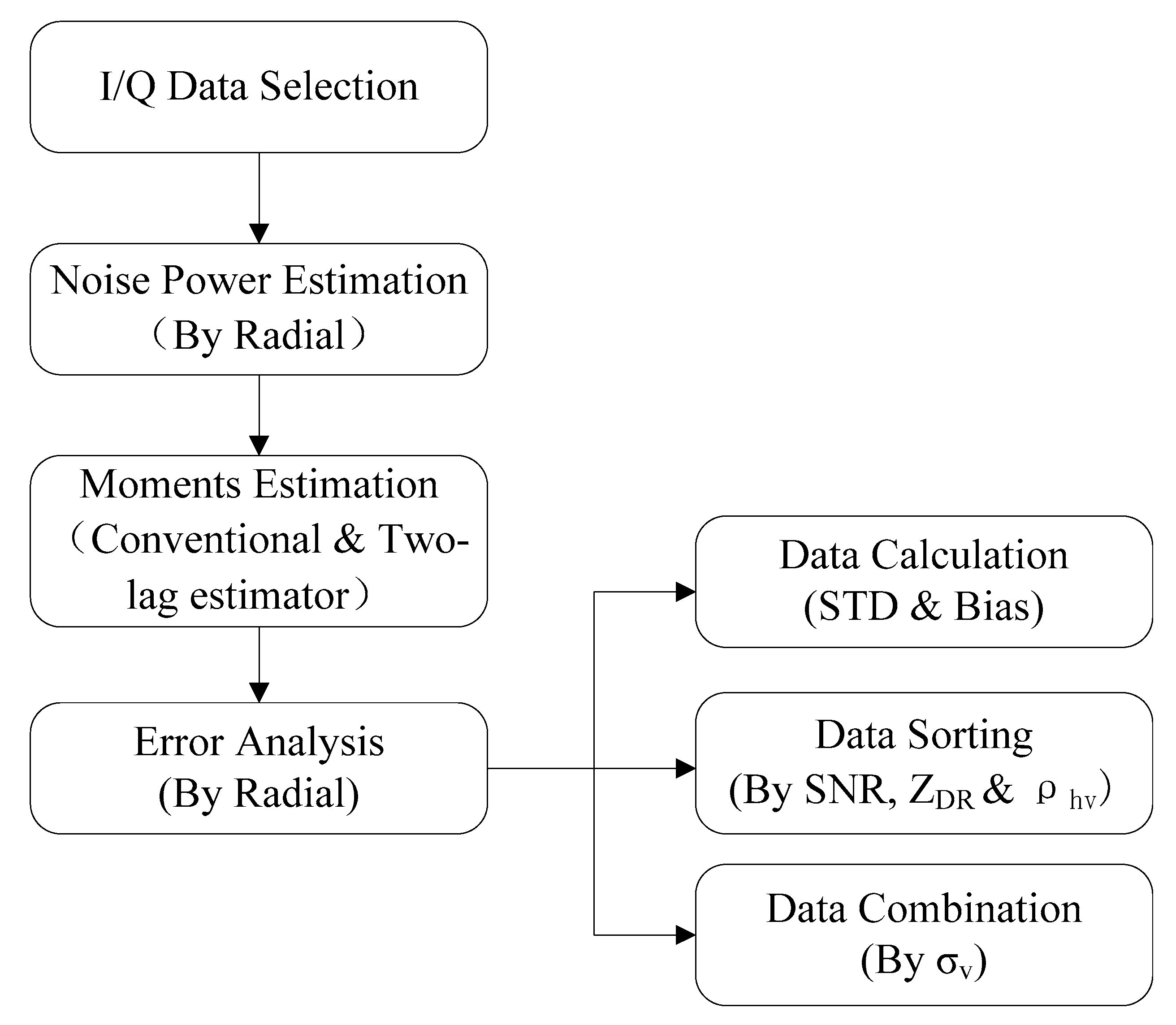
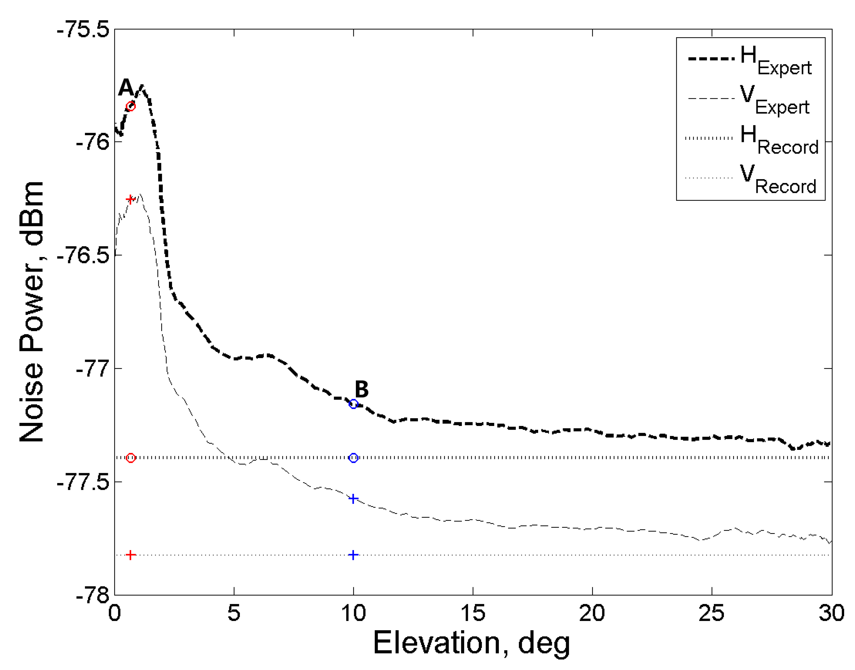
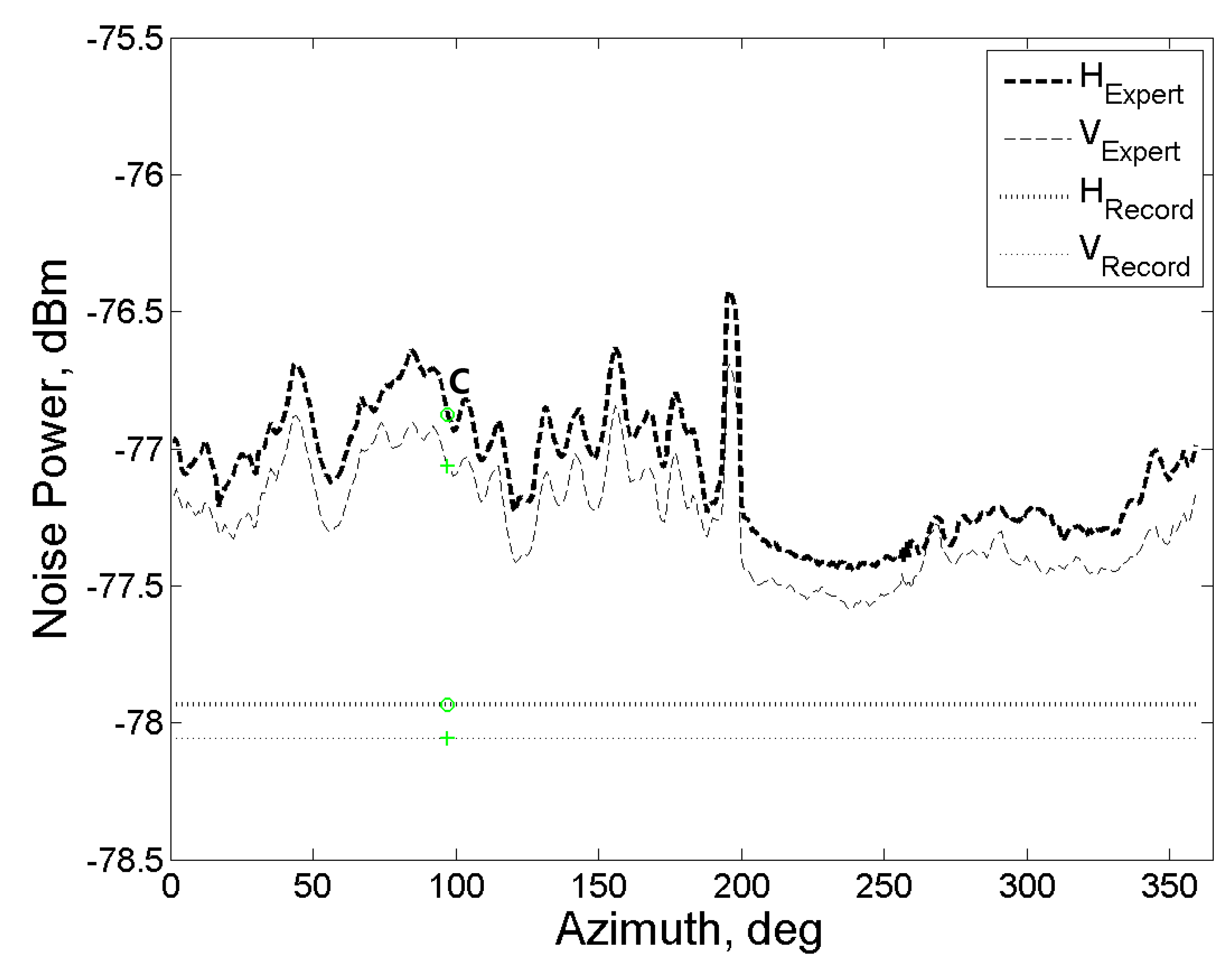
2.3. Error Analysis Method

Perturbation analysis [18,21] is used for theoretical analysis and terms for second-order of the Taylor expansion are retained. Then the theoretical data are compared with those from the radar scan data. The Taylor expansion in several variables from $\left|\widehat{R}\left(T_s\right)\right|$, $\left|\widehat{R}\left(2T_s\right)\right|$, to $\left|\widehat{R}\left(N{T}_s\right)\right|$, bias and variance of S_h can be found in Lei et al. ([24], Equations (15), (19), and (20)), which are shown as Equation (17) to (19), respectively. R(T_s) is the ACF and S^(N) is the signal power estimated by using N lags of ACF; n₁, …, n_N are the number of derivatives for each variable in the Taylor expansion. For theoretical analysis, parameters are set as follows, M = 64, T_s = 0.001 s, λ = 0.053 m, SNR = 10 dB (H channel), ρ_hv = 0.97, Z_DR = 1 dB, which corresponds to scan parameters of NJU-CPOL radar. Noise power biases for H and V channel are set as equal in theoretical analysis.

$$S^{\left(N\right)}\left[\left|\widehat{R}\left(T_s\right)\right|,\dots ,\left|\widehat{R}\left(N{T}_s\right)\right|\right]={\displaystyle \sum }_{n_1=0}^{\infty }\dots {\displaystyle \sum }_{n_N=0}^{\infty }\left\{\begin{array}{l}\frac{{\left[\left|\widehat{R}\left(T_s\right)\right|-\left|R\left(T_s\right)\right|\right]}^{n_1}\dots {\left[\left|\widehat{R}\left(T_s\right)\right|-\left|R\left(N{T}_s\right)\right|\right]}^{n_N}}{n_1!\dots n_N!}.\\ \left[\frac{{\partial }^{n_1+\dots +n_N}{S}^{\left(N\right)}}{\partial {\left|\widehat{R}\left(T_s\right)\right|}^{n_1}\dots \partial {\left|\widehat{R}\left(N{T}_s\right)\right|}^{n_N}}\right]\left[\left|R\left(T_s\right)\right|,\dots \left|R\left(N{T}_s\right)\right|\right]\end{array}\right\}$$

(17)

$$Bias\left[S^{\left(N\right)}\right]=\langle {\displaystyle \sum }_{n_1=0}^{\infty }\dots {\displaystyle \sum }_{n_N=0}^{\infty }\left\{\begin{array}{l}\frac{{\left[\left|\widehat{R}\left(T_s\right)\right|-\left|R\left(T_s\right)\right|\right]}^{n_1}\dots {\left[\left|\widehat{R}\left(T_s\right)\right|-\left|R\left(N{T}_s\right)\right|\right]}^{n_N}}{n_1!\dots n_N!}.\\ \left[\frac{{\partial }^{n_1+\dots +n_N}{S}^{\left(N\right)}}{\partial {\left|\widehat{R}\left(T_s\right)\right|}^{n_1}\dots \partial {\left|\widehat{R}\left(N{T}_s\right)\right|}^{n_N}}\right]\left[\left|R\left(T_s\right)\right|,\dots \left|R\left(N{T}_s\right)\right|\right]\end{array}\right\}\rangle$$

(18)

$$Var\left[S^{\left(N\right)}\right]=\langle {\left({\displaystyle \sum }_{n_1=0}^{\infty }\dots {\displaystyle \sum }_{n_N=0}^{\infty }\left\{\begin{array}{l}\frac{{\left[\left|\widehat{R}\left(T_s\right)\right|-\left|R\left(T_s\right)\right|\right]}^{n_1}\dots {\left[\left|\widehat{R}\left(T_s\right)\right|-\left|R\left(N{T}_s\right)\right|\right]}^{n_N}}{n_1!\dots n_N!}.\\ \left[\frac{{\partial }^{n_1+\dots +n_N}{S}^{\left(N\right)}}{\partial {\left|\widehat{R}\left(T_s\right)\right|}^{n_1}\dots \partial {\left|\widehat{R}\left(N{T}_s\right)\right|}^{n_N}}\right]\left[\left|R\left(T_s\right)\right|,\dots \left|R\left(N{T}_s\right)\right|\right]\end{array}\right\}\right)}^2\rangle$$

(19)

For estimator validation, a reference value should be given first. Previous studies show that there will be little bias or no bias in the conventional estimator for the four variables discussed in this paper if noise power is estimated without bias [24,34]. The “expert noise power” method can be used to get a more accurate noise power. It is calculated by visually identifying a flat section in the power profile that is recognized by ‘‘expert’’ determination to be free of the coherent signal [20]. The result of the conventional estimator with expert noise power is used as a reference (true) value, and is then compared with the conventional estimator with record noise power (measured by radar online calibration system) and the two-lag estimator.

Bias and standard deviation are calculated separately for the actual radar data. The standard deviation for the current gate is calculated through some adjacent gates, including the current gate and adjacent gates and bias is calculated by subtracting the “true value” gate by gate. True value is calculated by conventional estimators with expert noise power estimated in Level Ι (I/Q) data. Then, conventional estimators with record noise power are compared with two-lag estimators for S_h, Z_DR, σ_v and ρ_hv estimation. For the convenience of noise power estimation by the expert method, higher elevation data are selected (i.e., 7 degrees above), which is free from the coherent signal at the far range. As for different estimators, the standard deviation is different for conventional estimators and two-lag estimators, and the subtraction of these two estimators will be noisy if data are used gate by gate directly. For the same gate, the true value of each variable exists, such as σ_v, SNR and so on. As for bias calculation, the difference mainly depends on the performance of each estimator and more gates used here can reduce the fluctuation. While for standard deviation calculation, some adjacent gates are used and the true value of each variable may be different. As a result, more errors may be introduced when more gates are used. In order to minimize the fluctuation, several adjacent subtraction data are selected and then a median value is chosen as a bias for the current gate. In this work, the number of gates used for bias statistic is 31, which includesthe current gate, 15 gates beforeand 15 gates after the current gate. Standard deviation is obtained by radial, as discussed before, but only 3 adjacent gates are used for large amounts of data statistics. The flowchart of error statistics is shown in Figure 1.

3. Results

Two specific cases including stratiform precipitation and squall line precipitation using the conventional estimator and two-lag estimator are discussed in Section 3.1 firstly, and then a more common comparison between the two estimators through both theoretical analysis and radar data statistics is given in Section 3.2. The summary part is concluded in both sections. Ground clutter is not mitigated in estimator validation for the reason that all estimators are in the same conditions.

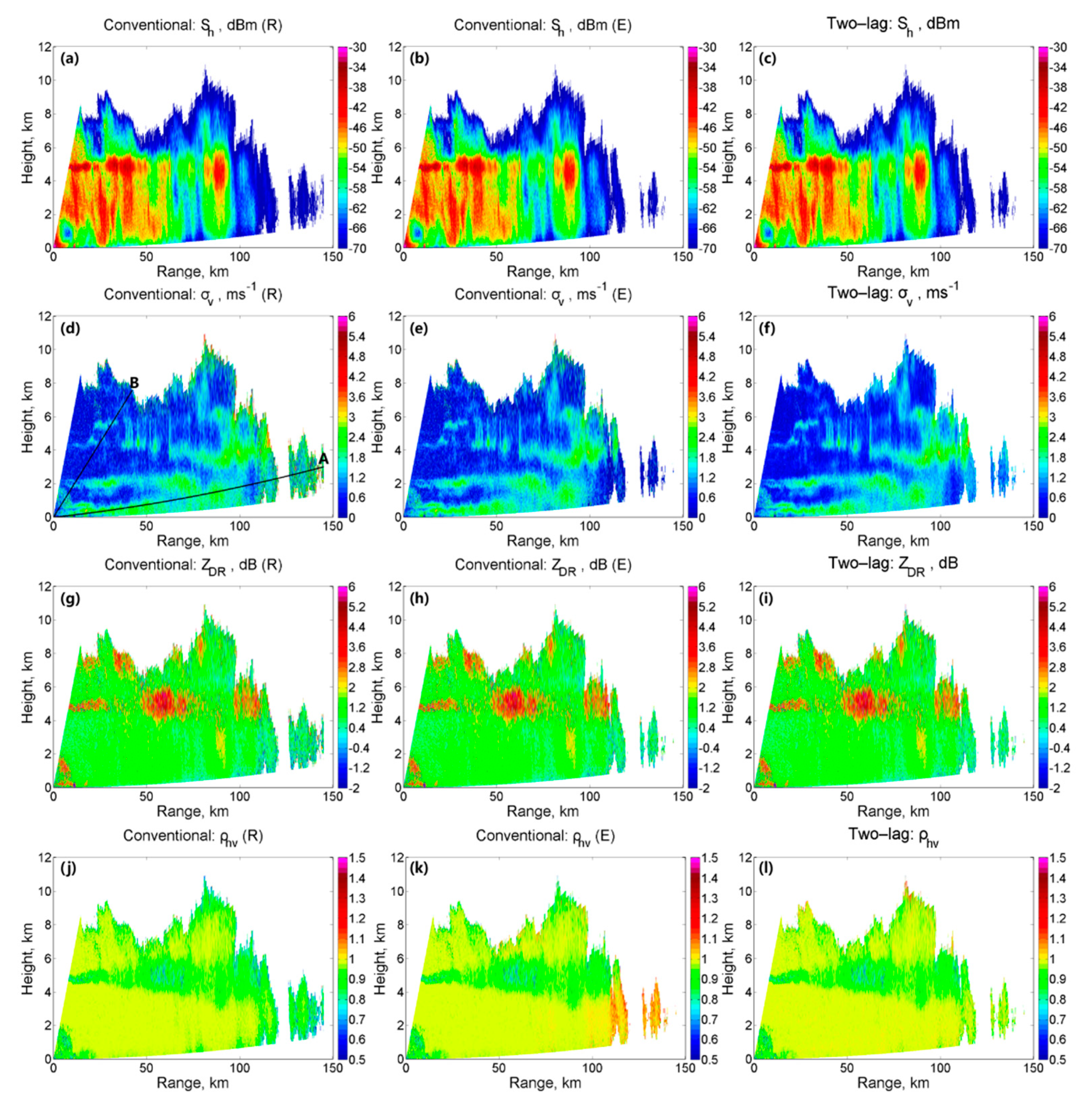
3.1. Case Studies and Results

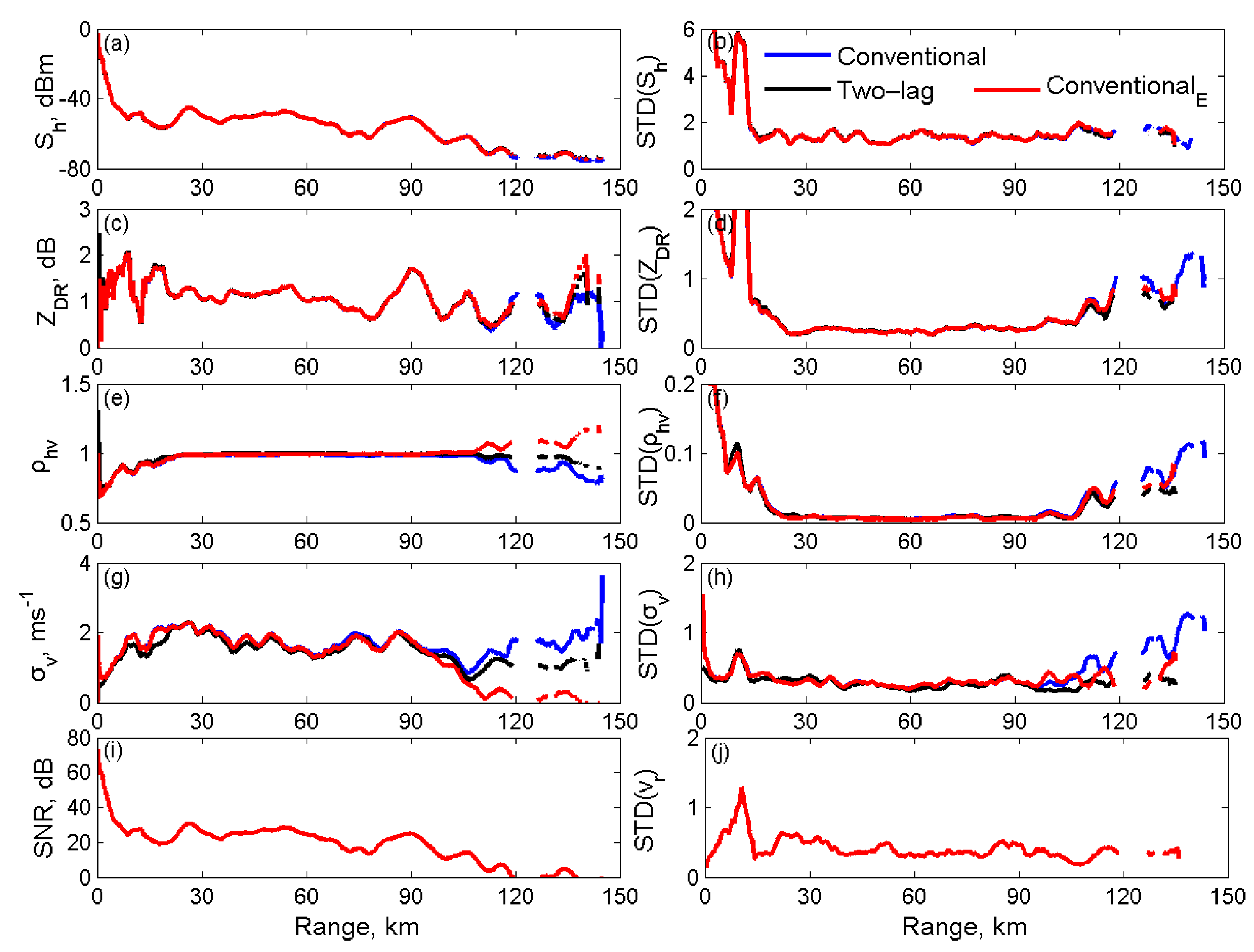
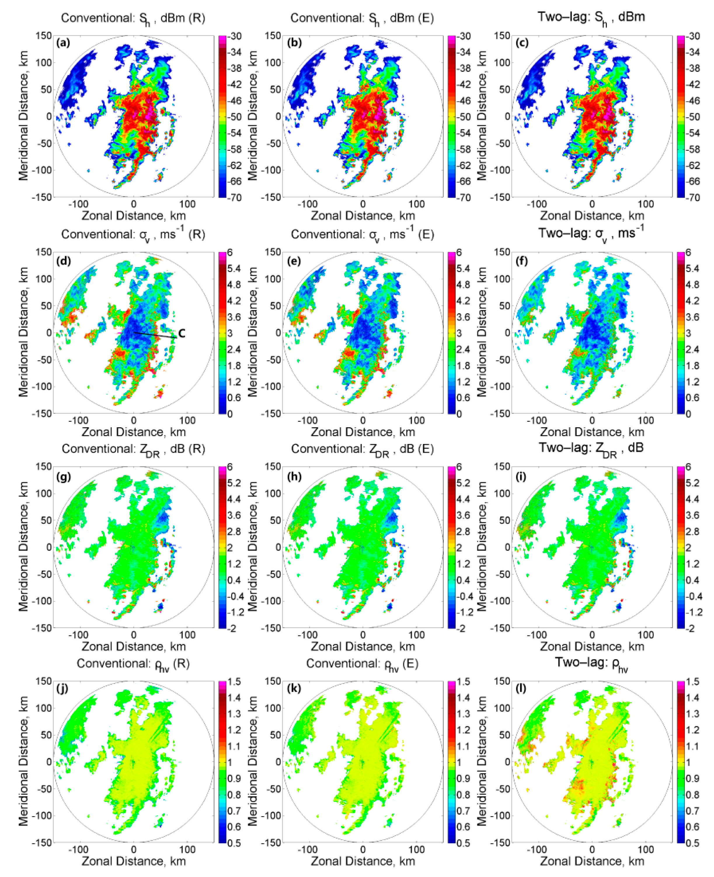
3.1.1. Case 1: Stratiform Precipitation

Figure 2 shows a stratiform precipitation case that occurred on 15 June 2014. Conventional estimators with record noise power are shown in the first column (as Figure 2a,d,g,j), labeled with letter ”R”; conventional estimators with expert noise power are shown in the middle column (as Figure 2b,e,h,k), labeled with letter ”E”; and two-lag estimators are shown in the right column (as Figure 2c,f,i,l). Among three estimators, the moment data differ more at far ranges such as 120 km to 150 km since the noise power used for moment estimation is different. Although the threshold of SNR is set to 0 dB for all estimators, the noise power is estimated by different methods which will cause difference especially when SNR is low. For S_h (Figure 2a–c) and Z_DR (Figure 2g–i) estimation, all these three estimators agree well except for the difference caused by the SNR threshold in this case. However, there are more differences in σ_v and ρ_hv estimation when SNR is low. For σ_v (Figure 2d–f), at the range of about 120 km to 150 km, the value from the conventional estimator with record noise is larger than those from the conventional estimator with expert noise power and two-lag estimator. This is because the record noise power is underestimated which will lead to an overestimation of σ_v. Similarly, this will lead to an underestimation of ρ_hv. However, there are still some data larger than 1 even if expert noise power is used in the conventional estimator when SNR is low. As for the two-lag estimator, little data is larger than 1 for ρ_hv estimation in the same conditions. Overall, results from the two-lag estimators in Figure 1 agree with the reference value better than the conventional estimator, and the main difference between the two-lag estimator and conventional estimator occurs at low SNR. Radial A (elevation 0.7 deg) and B (elevation 10.0 deg) are chosen for further analysis.

Noise powers for data illustrated in Figure 2 from the expert method (with subscript “Expert”) and online calibration system (with subscript “Record”) are shown in Figure 3. The maximum elevation angle of RHI for NJU-CPOL is 30 degrees. Symbols A and B in Figure 3 correspond to radials A and B in Figure 2, respectively. Circle and plus signs in Figure 3 show the noise power of expert value and record value for horizontal and vertical channels, respectively. The power difference between expert noise power and record noise power is large for low elevations and small for high elevations in both horizontal and vertical channels. At radial A, the record noise power is underestimated by 1.55 dB for H channel and 1.57 dB for V channel and; at radial B, the record noise power is underestimated by 0.24 dB for H channel and 0.25 dB for V channel. The ground clutter is not removed when the noise power is estimated by the expert method. As a result, ground clutter and thermal radiation may mainly contribute to the large noise power difference at low elevation, where ρ_hv is smaller and standard deviation of S_h, σ_v, Z_DR, ρ_hv, are larger than precipitation area (which can be seen in Figure 4).

S_h, Z_DR, ρ_hv, σ_v and their standard deviations for radial A are shown in Figure 4. In addition, SNR and STD(v_r) are also exhibited in Figure 4. The standard deviation for the current gate is calculated through five adjacent gates, including the current gate, and two gates before and after the current range gate. Too many gates used for standard deviation calculation at the current gate may be influenced more by other gates, such as clutter, melting layer and other non-precipitation echoes, especially when the SNRs differ greatly among all used gates. Conventional estimators calculated with expert noise power are shown in red color with subscription “E”, which are compared with conventional estimators with record noise power (blue color line) and two-lag estimators (black color line). The SNR shown in Figure 4i is calculated by expert noise power estimation and can be regarded as the true value. All the moments are smoothed using a moving average filter with a span of 50 to get a clear trend. Data near the radar are contaminated by clutter, and the standard deviation of each moment is higher than the weather echo. For weather echoes with SNR larger than 20 dB and σ_v less than 2 ms⁻¹, the moments and their standard deviations from different estimators are almost the same. However, if the spectrum width is larger than 2 ms⁻¹, the two-lag estimator has an underestimated σ_v compared to those of reference. When SNR is less than 20 dB and spectrum width less than 2 ms⁻¹, moments estimated from the two-lag estimator are closer to reference value than the conventional estimator in record noise power. Moreover, the standard deviation of each moment from the two-lag estimator is smaller than that of the conventional estimator. The STD(v_r) is less than 0.5 for the weather echo but can be more than 1 in the presence of ground clutter (see Figure 4j). For the conventional estimator, the obvious overestimation of the σ_v and underestimation of the ρ_hv can be seen when the SNR is less than 20 dB because of the significant biases from noise power measurement.

At radial B, the noise power difference between expert value and record value is 0.24 dB for H channel and 0.25 dB for V channel, which is smaller than those at radial A. As a result, the differences between the four moments estimated by conventional estimators as compared to those estimated by two-lag estimators are also very small for weather echo even if the SNR is low (Figure 5). The echo near radar is also affected by ground clutter, where the standard deviation of each moment is higher than that of weather echoes. The standard deviation of S_h (STD(S_h)) and Z_DR (STD(Z_DR)) is almost same at all range gates for both conventional and two-lag estimators, but standard deviation of ρ_hv (STD(ρ_hv)) from the two-lag estimator is smaller than conventional one where the SNR is less than 20 dB. For σ_v, the standard deviation of the two-lag estimator is smaller than the conventional estimator at all ranges. STD(v_r) is less than 0.5 for the pure weather echo, similar to radial A.

As shown in Figure 2, Figure 4, and Figure 5 in this stratiform precipitation case, most of the σ_v is less than 2 ms⁻¹, which is suitable for the two-lag estimator. In this situation, variables from the two-lag estimator agree with the reference value better than the conventional estimator with record noise power for the reason that there are some biases in record noise power. In addition, the standard deviation of the two-lag estimator for σ_v and ρ_hv is smaller than the conventional estimator, especially when the SNR is less than 20 dB. However, there is no obvious improvement of standard deviation for S_h and Z_DR estimation when the two-lag estimator is used.

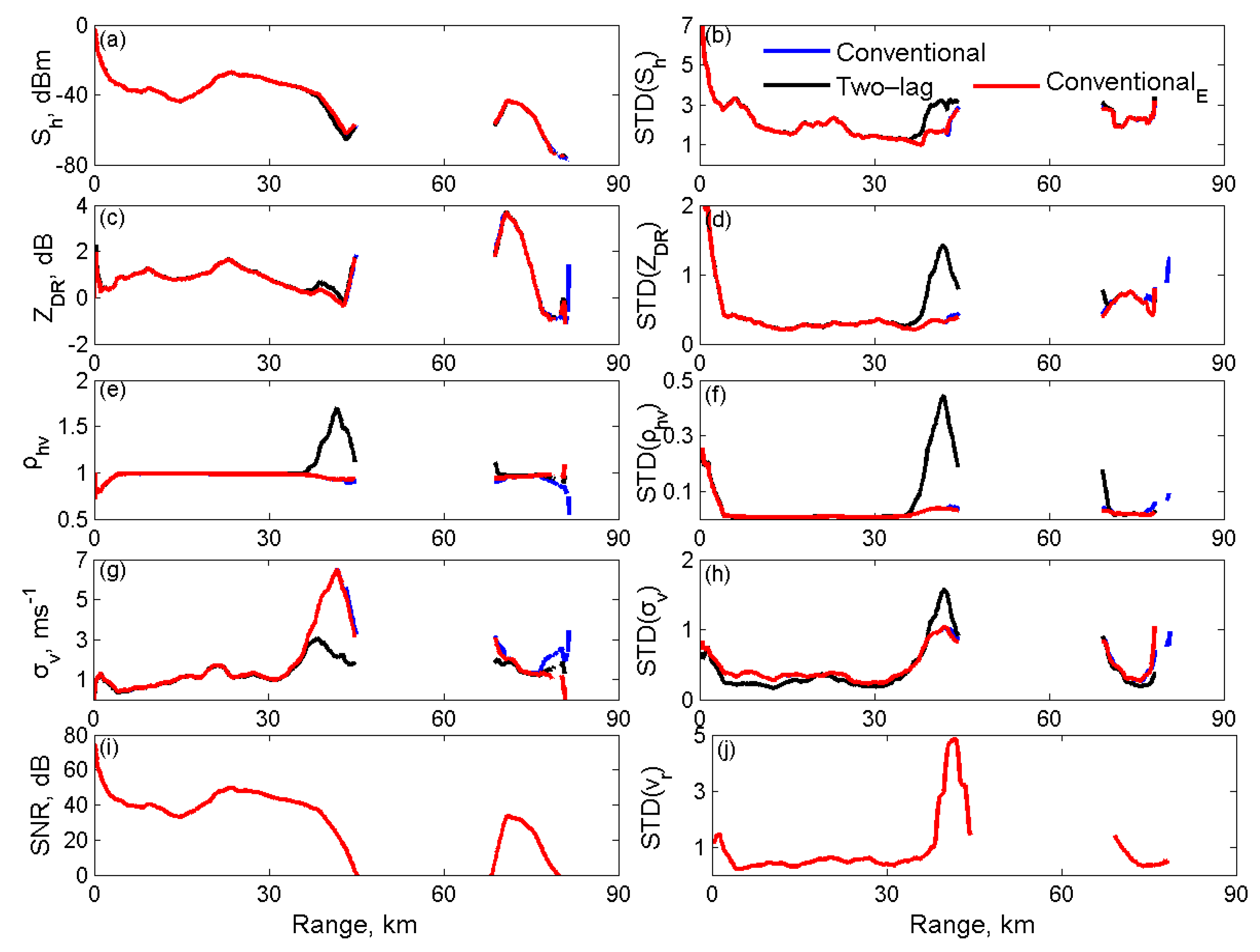
3.1.2. Case 2: Squall Line Precipitation

Figure 6 shows another case that occurred on 30 July 2014, which is a squall line precipitation. Results for the conventional estimators with record noise power are shown in the first column (as Figure 6a,d,g,j); the results for conventional estimators with expert noise power (as reference value) are shown in the middle column (as Figure 6b,e,h,k); and the results for two-lag estimators are shown in the right column (as Figure 6c,f,i,l). In this case, echoes with large spectrum width (larger than 3 ms⁻¹) are detected in many regions. For the two-lag estimator, the obvious underestimation of σ_v and overestimation of ρ_hv can be seen among these high spectrum width areas. For NJU-CPOL radar, ACF/CCF at lag 2 cannot be used when the spectrum width is large (larger than 2 ms⁻¹), because it will cause more error to moments estimation [24]. When the spectrum width is small (less than 2 ms⁻¹), estimates with the two-lag estimators agree with reference values better than that with the conventional one, especially when SNR is lower than 20 dB. Radial C is chosen for detailed analysis, which penetrates the squall line.

The noise power of each radial estimated by expert method for the whole PPI is shown in Figure 7. In addition, noise power measured by the real-time radar calibration system is shown for comparison. Like RHI data shown in Figure 2, noise power estimated by the expert method is also varying at different azimuths. The difference of noise power between the expert method and record value at radial C is 0.88 dB for the H channel and 0.77 dB for the V channel. That is to say, the noise power from the real-time calibration system is underestimated for both channels. For conventional estimators, the underestimation of noise power will lead to an overestimation of σ_v and underestimation of ρ_hv.

Detailed analysis for radial C is shown in Figure 8. Moments selected here are the same as Figure 4 and Figure 5, including S_h, Z_DR, ρ_hv, σ_v and their standard deviations, SNR and STD(v_r). Different from radial A and B, radial C penetrates the squall line area that has a large spectrum width (larger than 6 ms⁻¹). Obvious biases for moments estimated by two-lag estimators can be seen at the large spectrum width area, and their standard deviations are much bigger than the conventional one. The unrealistic significant large ρ_hv from the two-lag estimator in the area of large spectrum width (as shown in Figure 8e) is due to the lack of enough usable lags. More errors will be brought in when the two-lag estimator is used in such a condition. When σ_v is larger than 6 ms⁻¹, the maximum usable lag number is less than 1. That is also why the obvious biases and large standard deviations of two-lag estimators exhibit at large spectrum width areas. In addition, as indicated in Figure 8j, the STD(v_r) is larger than 1 ms⁻¹ when σ_v is larger than 3 ms⁻¹.

A summary of the standard deviations for radial A, B, and C are shown in Figure 9. The distribution of standard deviations for S_h, Z_DR, σ_v, and ρ_hv from conventional estimators and two-lag estimators are shown in Figure 9a–d, respectively. The larger the normalized frequency, the more amount of specific standard deviation. For S_h and Z_DR, the distribution of standard deviation is almost the same, but for σ_v and ρ_v, it shows an obvious difference from conventional estimators and two-lag estimators. The largest normalized frequency of spectrum width is 0.44 for the two-lag estimator and 0.32 for the conventional estimator, corresponding to standard deviations of 0.2 and 0.3, respectively. This means that the standard deviation of the two-lag estimator is smaller than the conventional estimator for σ_v. For ρ_hv, the standard deviation of the biggest normalized frequency is 0.001 for both conventional and two-lag estimators. However, the biggest normalized frequency is 0.63 for the two-lag estimator and 0.54 for the conventional estimator. That is to say, the standard deviation of the two-lag estimator is smaller than the conventional estimator for ρ_hv, too. In summary, from radials A, B and C, it is concluded that two-lag estimators perform better in σ_v and ρ_hv estimation and have equal performance in S_h and Z_DR estimation compared with conventional estimators.

Another comparison is shown in Figure 10, which is also calculated from radial A, B, and C. The difference for S_h, Z_DR, σ_v, and ρ_hv of the conventional estimator and the two-lag estimator is calculated through subtracting reference value gate by gate, which is marked by “Diff” in the label of axial y. Only the data with the SNR less than 20 dB are taken into account and then are sorted by reference σ_v. Overall, except for Z_DR, the difference between the two-lag estimator and the reference value is smaller than the conventional one when σ_v is less than 2 ms⁻¹, which accords with previous research [24]. However, there is little improvement in the two-lag estimator for Z_dr estimation in these three radial data. The lack of useful lags accounts for the large value from the two-lag estimator in Figure 10 when σ_v is large. Moving average filter with a span of 100 is used in the data analysis which can show a clearer trend.

3.2. Results Based on IOPs Data

The performance of S_h, Z_DR, σ_v, and ρ_hv estimated by conventional and two-lag estimators examined through two specific cases are discussed in Section 3.1 and in this section, more data are used for performance validation. For actual radar data statistics, 1852 PPI data are selected from 15 June, 21 June, 25 June, 4 July, 12 July, 17 July, 24 July, and 30 July 2014 including many types of precipitation, such as stratiform, Meiyu front, squall line and so on. The method for error analysis is discussed in Section 2.3.

Bias and standard deviation of four variables (S_h, σ_v, Z_DR, ρ_hv) from both theoretical analysis and actual data are shown in Figure 11. Theoretical bias for S_h of the conventional estimator is depending on noise power estimation error, which is not given in Figure 11a.

Error analysis of S_h is shown in Figure 11a,b. The actual biases of the conventional estimator from radar data are almost the same at different spectrum widths, while the biases of the two-lag estimator vary with spectrum width. When spectrum width is less than 1 ms⁻¹, the bias of the two-lag estimator is close to the theoretical value and smaller than those from the conventional estimator. If the spectrum width is larger than 2 ms⁻¹, the bias of the two-lag estimator from actual data has a significant negative value, which is different from the theoretical value. STD(S_h) for the conventional estimator and two-lag estimator is almost same for both theoretical and actual data when the spectrum width is less than 3 ms⁻¹, but differs at each spectrum width, especially when the spectrum width is less than 0.5 ms⁻¹. One reason may come from the Taylor expansion, which is only valid when the estimated value is close to the true value.

Bias and standard deviation of σ_v are shown in (c) and (d) of Figure 11. For the theoretical analysis of the conventional estimator, the bias of noise power is set to −1 dB (underestimation). Actual bias is given in Figure 11c, which shows the same trend as the theoretical value for both conventional and two-lag estimators. The actual bias for the conventional estimator is smaller than the theoretical value for the reason that the bias of measured noise power is less than 1 dB. The standard deviation is shown in Figure 11d, which also shows the same trend as the theoretical value. The main reason for the large difference at a spectrum less than 0.5 ms⁻¹ is also the Taylor expansion.

Figure 11e,f show the bias and standard deviation of Z_DR. Theoretical bias and standard deviation of Z_DR are almost the same when the spectrum width is less than 2 ms⁻¹, and are smaller for the conventional estimator when the spectrum width is larger than 3 ms⁻¹. For actual data, bias from the conventional estimator is negative and varies little with the spectrum width, but varies more with spectrum width for the two-lag estimator. Standard deviation from actual data shows that the value from the conventional estimator is smaller than the two-lag estimator, but very close to each other when the spectrum width is less than 2 ms⁻¹.

The performance of ρ_hv for the conventional estimator and two-lag estimator is shown in Figure 11g,h. Biases and standard deviations from actual data show the same trend and are close to theoretical values. For theoretical analysis, the noise power is set equal for both channels, but different for real data. This is the main reason for the difference in the bias between the theoretical and statistic value of the conventional estimator. From real data, the result shows that the bias of the two-lag estimator is smaller when the spectrum width is less than 1 ms⁻¹. Besides, the standard deviation is smaller when the spectrum width is less than 2.5 ms⁻¹ compared to the conventional estimator.

Overall, results from observed radar data show good agreement with those from theoretical analysis. The two-lag estimator has a better performance in σ_v and ρ_hv estimation and has similar performance in S_h and Z_DR estimation when the spectrum width is less than 2 ms⁻¹. As mentioned, two reasons may account for the little difference between theoretical value and real value: the Taylor expansion and the limited samples for performance evaluation.

4. Discussion

The data quality of the four radar variables (S_h, σ_v, Z_DR, ρ_hv) discussed in Section 3 show that the two-lag estimator performs better than the conventional one in σ_v and ρ_hv estimation, especially when SNR is lower than 20 dB, and have similar performance in S_h and Z_DR estimation when spectrum width is less than 2 ms⁻¹. Usable lags are less than 2 when the spectrum width is larger than 2 ms⁻¹ for the scan parameters used in NJU-CPOL. As a result, the two-lag estimator cannot be used in such situations. In order to improve radar data quality in weak echo with low SNR, a hybrid method is introduced and implemented on NJU-CPOL.

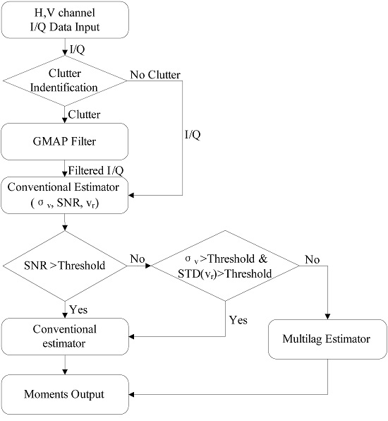
4.1. The Hybrid Algorithm

The hybrid method is based on both the conventional estimator and the multilag estimator. The basic principle is that all lags beside lag 0 of ACF are used for moment estimation according to the maximum usable lag number, which is determined by spectrum width and other radar parameters (such as wavelength, PRT). As analyzed in Section 3, the performance of the conventional estimator and two-lag estimator is almost the same when SNR is larger than 20 dB. In addition, the calculation process of the conventional estimator is simpler than that of the multilag estimator. As a result, the conventional estimator is used when SNR is large and the multiage estimator is used with low SNR and suitable usable lags. The flowchart of the hybrid algorithm is shown in Figure 12. Three moments including SNR, σ_v, and v_r are first estimated by conventional estimators, and then these moments are acted as thresholds. As for σ_v, it may be not reliable if noise power is estimated with biases when SNR is low. In this case, STD(v_r) is used as a supplement. As shown in Section 2, STD(v_r) is far less than 1 ms⁻¹ when spectrum width is less than 2 ms⁻¹ for weather echo. Besides, v_r is estimated with lag 1 in the conventional estimator and can be regarded as not influenced by noise. Therefore, the combination of σ_v and STD(v_r) will be a good indicator for real large spectrum width in weather echoes with low SNRs. The thresholds here for SNR, σ_v, and STD(v_r) are 15 dB, 2 ms⁻¹, and 0.6 ms⁻¹, respectively, which are selected according to the results of performance analysis.

4.2. Case Study and Results

A squall line precipitation case estimated by the hybrid method is shown in Figure 13. Data are obtained by NJU-CPOL radar on 30 July 2014. A PPI with an elevation of 1.5 degrees is chosen because it can detect a clear squall line precipitation. As discussed, the conventional estimator with record noise power has significant biases for σ_v and ρ_hv estimation when SNR is low due to the bias of noise power estimation, and the two-lag estimator performs poorly when the spectrum width is large. That is to say, there are obvious biases in moment estimation based on both conventional and two-lag estimators. As shown in Figure 13, the hybrid method shows a more reasonable result than those from the conventional or two-lag estimators in Figure 6. At the range of about 120 km to 150 km, the correlation coefficient from the hybrid method is around 1 while values from the conventional estimator exhibit an obvious decrease (0.5 to 1 decreasing with reduced SNR) due to the noise power estimation biases. For σ_v estimation in the same range, the value from the conventional estimator with record noise power is larger than those from the hybrid method and reference value because underestimated bias will lead to an overestimation on σ_v. In addition, there are no obvious biases in σ_v and ρ_hv in the hybrid method while existing in the two-lag estimator when the spectrum width is larger than 2 ms⁻¹. However, the improvement for S_h and Z_DR estimation is not as significant as these for σ_v and ρ_hv in this hybrid method.

Biases of the conventional and the hybrid estimators for the PPI data of the squall line precipitation case are shown in Figure 14. A reference value is also obtained by the conventional estimator with noise power estimated by the expert method. In general, the biases of the hybrid method are smaller than those from the conventional estimator and the difference between the two estimators increases while SNR decreases. That is, the hybrid method performs better than the conventional estimator. Taking SNR = 10 dB as an example, the biases of S_h from the hybrid method and conventional estimator are 0.08 dB and 0.13 dB, respectively. The biases are 0.002 dB and −0.01 dB for Z_DR, 0.19 ms⁻¹ and 0.24 ms⁻¹ for σ_v, −0.016 and −0.029 for ρ_hv from the hybrid method and conventional estimator with SNR equal to 10 dB, respectively. If the biases of noise power increase, the biases of the conventional estimator will also increase. A moving average filter with a span of 50 is used in the bias analysis which can show a clearer trend.

Biases and standard deviations from the conventional estimator and hybrid estimator are shown in Figure 15 and Figure 16, respectively. All the data used here are the same as Figure 10. Different from Figure 14, σ_v is used as the control variable and SNR is chosen as 10 dB. Based on the results of biases and standard deviations, improved performance for σ_v and ρ_hv can be obtained by using the hybrid estimator at SNR = 10 dB. The performance for S_h and Z_DR estimation is almost the same as the conventional estimator for the reason that higher elevation data are used for statistics. The bias of noise power estimation is small at higher elevation due to the estimated method. Moving average filter with a span of 50 is used in the error analysis which can show a clearer trend.

5. Conclusions

In this paper, a multilag estimator is implemented on NJU-CPOL and the performance of the multilag estimator and conventional estimator is examined through measurements collected during the OPACC field campaign. According to the parameters of NJU-CPOL, the two-lag estimator is used in performance comparison and validation. Based on the performance of various estimators, a hybrid method is introduced, which has improved performance in moment estimation for weak weather echo.

For the performance validation, a stratiform precipitation case and a squall line case are used. In the former case, there are few echoes with large spectrum width (i.e., larger than 2 ms⁻¹), but the maximum σ_v in the convective region exceeds 6 ms⁻¹ in the latter case. Results from these two cases show that the two-lag estimator performs better than the conventional estimator when the spectrum width is less than 2 ms⁻¹, especially for weak weather echoes. However, there will be significant biases in the two-lag estimator if it is used in a convective region. Performance from more IOPs data shows similar results. A method of bias and standard deviation calculation is proposed in this study to quantify the estimator performance. That is, true value (reference value) is calculated by the conventional estimator with expert noise power, and then the biases can be obtained by subtraction of reference value for the two-lag or conventional estimator with record noise power. The standard deviation of each moment is calculated by radial with five adjacent gates. In general, the error results from radar data statistics agree well with these from the theoretical value obtained by perturbation analysis, but a minor difference still exists between the two methods. Two reasons mainly account for this minor difference: one is the Taylor expansion, which is kept to the second derivative term for simplicity; and the other is the limited number of samples used in the calculation of performance statistics. The Taylor expansion used for perturbation analysis is only valid when the estimated value is close to the true value. However, the difference between the estimated value and true value will be enlarged with the decrease of SNR and this may not yield the small relative errors required for the Taylor expansion to be valid. For actual data statistics, as many as 70,000 samples can be used with specific SNR, σ_v, Z_DR and ρ_hv when spectrum width is less than 3 ms⁻¹, but much fewer samples can be used when spectrum width is close to 4 ms⁻¹.

After careful consideration of the performance of the conventional estimator and multilag estimator, a hybrid estimator is proposed. All lags besides lag 0 of ACF are used for moment estimation in this hybrid algorithm. Large number lags can be used to reduce noise effect, whereas low number lags can be applied in high spectrum width situations. Clutter identification with the SBC approach and GMAP are used for clutter mitigation in this hybrid estimator. In order to confirm the high spectrum width region with low SNR, STD(v_r) is used as an indicator, which is less than 1 ms⁻¹ with a small spectrum width but can be larger than 1 ms⁻¹ with a large spectrum width for weather echoes. For NJU-CPOL, the threshold of STD(v_r) is 0.6. A squall line precipitation case shows that the hybrid method has a bias improvement of 0.05 dB for S_h, 0.012 dB for Z_DR, 0.05 ms⁻¹ for σ_v, and 0.013 for ρ_hv, compared with conventional estimator when SNR is equal to 10 dB. The improvement will be more significant if SNR decreases or the biases of noise power used in conventional estimation increase. In addition, there are no additional requirements to implement this hybrid method, which should be considered for both operational radars and non-operational research radars. It is expected that a better performance can be achieved if the method is applied to S-band polarimetric radars for which the useable lags are twice that for C-band radars.

However, as no weighted blending is used in this hybrid method, small steps may exist in the final variables. Practical implementations should focus on this aspect, especially during different hydrometeor conditions.

References

1. Vivekanandan, J.; Zrnic, D.S.; Ellis, S.M.; Oye, R.; Ryzhkov, A.V.; Straka, J. Cloud Microphysics Retrieval Using S-Band Dual-Polarization Radar Measurements. Bull. Am. Meteorol. Soc. 1999, 80, 381–388. [Google Scholar] [CrossRef]
2. Bringi, V.N.; Chandrasekar, V. Polarimetric Doppler Weather Radar: Principles and Applications; Cambridge University Press: Cambridge, UK, 2001; p. 636. [Google Scholar]
3. Zrnić, D.S.; Ryzhkov, A. Advantages of rain measurements using specific differential phase. J. Atmos. Ocean. Technol. 1996, 13, 454–464. [Google Scholar] [CrossRef] [Green Version]
4. Chen, H.; Chandrasekar, V.; Bechini, R. An Improved Dual-Polarization Radar Rainfall Algorithm (DROPS2.0): Application in NASA IFloodS Field Campaign. J. Hydrometeorol. 2017, 18, 917–937. [Google Scholar] [CrossRef]
5. Groginsky, H.L.; Glover, K.M. Weather radar canceller design. In Proceedings of the 19th Conference on Radar Meteorology, Miami Beach, FL, USA, 15–18 April 1980. [Google Scholar]
6. Meischner, P. Weather Radar Principles and Advanced Applications; Springer: Berlin/Heidelberg, Germany, 2002; p. 337. [Google Scholar]
7. Lee, R.; Deruma, G.; Joss, J. Intensity of ground clutter and of echoes of anomalous propagation and its elimination. In Proceedings of the 27th Conference on Radar Meteorology, Vail, CO, USA, 9–13 October 1995; pp. 651–652. [Google Scholar]
8. Kessinger, C.; Ellis, S.; Andel, J.V. The radar echo classifier: A fuzzy logic algorithm for the WSR-88D. In Proceedings of the Third Conference on Artificial Intelligence Applications to the Environmental Science, Long Beach, CA, USA, 9–13 February 2003; American Meteorological Society: Boston, MA, USA, 2003. [Google Scholar]
9. Steiner, M.; Smith, A. Use of Three-Dimensional Reflectivity Structure for Automated Detection and Removal. J. Atmos. Ocean. Technol. 2002, 19, 673–686. [Google Scholar] [CrossRef]
10. Hubbert, J.C.; Dixon, M.; Ellis, S.M.; Meymaris, G. Weather Radar Ground Clutter. Part I: Identification, Modeling, and Simulation. J. Atmos. Ocean. Technol. 2009, 26, 1165–1180. [Google Scholar] [CrossRef]
11. Hubbert, J.C.; Dixon, M.; Ellis, S.M. Weather Radar Ground Clutter. Part II: Real-Time Identification and Filtering. J. Atmos. Ocean. Technol. 2009, 26, 1181–1197. [Google Scholar] [CrossRef]
12. Siggia, A.D.; Passarelli, R.E. Gaussian model adaptive processing (GMAP) for improved ground clutter cancellation and moment calculation. Proc. ERAD 2004, 2, 421–424. [Google Scholar]
13. Zhang, G.; Li, Y.; Doviak, R.J.; Priegnitz, D.; Carter, J.; Curtis, C.D. Multipatterns of the National Weather Radar Testbed Mitigate Clutter Received via Sidelobes. J. Atmos. Ocean. Technol. 2011, 28, 401–409. [Google Scholar] [CrossRef]
14. Li, Y.; Zhang, G.; Doviak, R.J. Ground Clutter Detection Using the Statistical Properties of Signals Received With a Polarimetric Radar. IEEE Trans. Signal Process. 2014, 62, 597–606. [Google Scholar] [CrossRef]
15. Melnikov, V.M.; Zhang, P.; Zrnic, D.S.; Ryzhkov, A. Recombination of Super Resolution Data and Ground Clutter Recognition on the Polarimetric WSR-88D; NSSL: Norman, OK, USA, 2008. [Google Scholar]
16. Golbon-Haghighi, M.-H.; Zhang, G. Detection of Ground Clutter for Dual-Polarization Weather Radar Using a Novel 3D Discriminant Function. J. Atmos. Ocean. Technol. 2019, 36, 1285–1296. [Google Scholar] [CrossRef]
17. Doviak, R.J.; Zrnić, D.S. Doppler Radar and Weather Observations, 2nd ed.; Dover Publication: Mineola, NY, USA, 2006; p. 562. [Google Scholar]
18. Melnikov, V.M.; Zrnić, D.S. Autocorrelation and Cross-Correlation Estimators of Polarimetric Variables. J. Atmos. Ocean. Technol. 2007, 24, 1337–1350. [Google Scholar] [CrossRef]
19. Fang, M.; Doviak, R.J.; Melnikov, V. Spectrum Width Measured by WSR-88D: Error Sources and Statistics of Various Weather Phenomena. J. Atmos. Ocean. Technol. 2004, 21, 888–904. [Google Scholar] [CrossRef]
20. Ivić, I.R.; Curtis, C.; Torres, S.M. Radial-Based Noise Power Estimation for Weather Radars. J. Atmos. Ocean. Technol. 2013, 30, 2737–2753. [Google Scholar] [CrossRef]
21. Zhang, G.; Doviak, R.J.; Vivekanandan, J.; Brown, W.O.J.; Cohn, S.A. Performance of correlation estimators for spaced-antenna wind measurement in the presence of noise. Radio Sci. 2004, 39, 1–16. [Google Scholar] [CrossRef] [Green Version]
22. Warde, D.A.; Torres, S.M. Spectrum Width Estimation Using Matched Autocorrelations. IEEE Geosci. Remote Sens. Lett. 2017, 14, 1661–1664. [Google Scholar] [CrossRef]
23. Ivić, I.R. A Technique to Improve Copolar Correlation Coefficient Estimation. IEEE Geosci. Remote Sens. Lett. 2016, 54, 5776–5800. [Google Scholar] [CrossRef]
24. Lei, L.; Zhang, G.; Doviak, R.J.; Palmer, R.; Cheong, B.L.; Xue, M.; Cao, Q.; Li, Y. Multilag Correlation Estimators for Polarimetric Radar Measurements in the Presence of Noise. J. Atmos. Ocean. Technol. 2012, 29, 772–795. [Google Scholar] [CrossRef] [Green Version]
25. Cao, Q.; Zhang, G.; Palmer, R.D.; Knight, M.; May, R.; Stafford, R.J. Spectrum-Time Estimation and Processing (STEP) for Improving Weather Radar Data Quality. IEEE Geosci. Remote Sens. Lett. 2012, 50, 4670–4683. [Google Scholar] [CrossRef]
26. Xue, M. Preface to the Special Issue on the “Observation, Prediction and Analysis of severe Convection of China” (OPACC) National “973” Projec. Adv. Atmos. Sci. 2016, 33, 1099–1101. [Google Scholar] [CrossRef]
27. Vaisala. User’s Manual of RVP900TM Digital Receiver and Signal Processor (M211322EN-B); Vaisala: Vantaa, Finland, 2013; p. 478. [Google Scholar]
28. Doviak, R.J.; Bringi, V.; Ryzhkov, A.; Zahrai, A.; Zrnić, D. Considerations for Polarimetric Upgrades to Operational WSR-88D Radars. J. Atmos. Ocean. Technol. 2000, 17, 257–278. [Google Scholar] [CrossRef]
29. Zhang, G. Weather Radar Polarimetry; CRC Press: Boca Raton, FL, USA, 2016; p. 322. [Google Scholar]
30. Melnikov, V.M.; Doviak, R.J. Spectrum Widths from Echo Power Differences Reveal Meteorological Features. J. Atmos. Ocean. Technol. 2002, 19, 1793–1810. [Google Scholar] [CrossRef]
31. Luo, Y.; Chen, Y. Investigation of the predictability and physical mechanisms of an extreme-rainfall-producing mesoscale convective system along the Meiyu front in East China: An ensemble approach. J. Geophys. Res. Atmos. 2015, 120, 10593–10618. [Google Scholar] [CrossRef]
32. Sachidananda, M.; Zrnic, D.S. ZDR measurement considerations for a fast scan capability radar. Radio Sci. 1985, 20, 907–922. [Google Scholar] [CrossRef]
33. Sachidananda, M.; Zrnic, D.S. Differential propagation phase shift and rainfall rate estimation. Radio Sci. 1986, 21, 235–247. [Google Scholar] [CrossRef]
34. Melnikov, V.M.; Zrnic, D.S. Simultaneous Transmission Mode for the Polarimetric WSR-88D: Statistical Biases and Standard Deviations of Polarimetric Variables; NOAA/NSSL Report; NOAA: Silver Spring, MD, USA; NSSL: Norman, OK, USA, 2004; p. 84. [Google Scholar]
Figure 1. Flowchart of error statistic using I/Q data collected by NJU-CPOL.
Remotesensing 12 00180 g001
Figure 2. Comparison of conventional estimators (left and middle column) and two-lag estimators (right column). Four rows show Sh, σv, ZDR, and ρhv, respectively. Letter R in brackets means that record noise power is used and letter E means that expert noise power is used. (a) Sh (conventional, record noise power); (b) Sh (conventional, expert noise power); (c) Sh (two-lag); (d) σv (conventional, record noise power); (e) σv (conventional, expert noise power); (f) σv (two-lag); (g) ZDR (conventional, record noise power); (h) ZDR (conventional, expert noise power); (i) ZDR (two-lag); (j) ρhv (conventional, record noise power); (k) ρhv (conventional, expert noise power); and (l) ρhv (two-lag). Data are collected on 15 June 2014, 1203UTC, Az = 340° in stratiform precipitation.
Remotesensing 12 00180 g002
Figure 3. Noise power for RHI scan data showed in Figure 2 resulting from H and V channels. Radial A and B are marked respectively. Subscript “Expert” means that noise power is estimated by the expert method and subscript “Record” means that noise power is measured by the radar online calibration system. It can be seen that the power difference between expert noise power and record noise power is large for low elevations and small for high elevations in both horizontal and vertical channels. At radial A, the record noise power is underestimated by 1.55 dB for H channel and 1.57dB for V channel and; at radial B, the record noise power is underestimated by 0.24 dB for H channel and 0.25 dB for V channel.
Remotesensing 12 00180 g003
Figure 4. Comparison between conventional estimators and two-lag estimators for radial A. Four rows show Sh, σv, ZDR, ρhv and their standard deviation, respectively. SNR and STD(vr) are given in the fifth row. (a) Sh; (b) STD(Sh); (c) ZDR; (d) STD(ZDR); (e) ρhv; (f) STD(ρhv); (g) σv; (h) STD(σv); (i) SNR; and (j) STD(vr).
Remotesensing 12 00180 g004
Figure 5. Comparison between conventional estimators and two-lag estimators for radial B. Four rows show Sh, σv, ZDR, ρhv and their standard deviation, respectively. The SNR and standard deviation of vr are given in the fifth row. (a) Sh; (b) STD(Sh); (c) ZDR; (d) STD(ZDR); (e) ρhv; (f) STD(ρhv); (g) σv; (h) STD(σv); (i) SNR; and (j) STD(vr).
Remotesensing 12 00180 g005
Figure 6. Comparison of conventional estimators (left and middle column) and two-lag estimators (right column). Four rows show Sh, σv, ZDR, and ρhv, respectively. Letter R in brackets means that record noise power is used and letter E means that expert noise power is used. (a) Sh (conventional, record noise power); (b) Sh (conventional, expert noise power); (c) Sh (two-lag); (d) σv (conventional, record noise power); (e) σv (conventional, expert noise power); (f) σv (two-lag); (g) ZDR (conventional, record noise power); (h) ZDR (conventional, expert noise power); (i) ZDR (two-lag); (j) ρhv (conventional, record noise power); (k) ρhv (conventional, expert noise power); and (l) ρhv (two-lag). Data are collected on 30 July 2014, 1410UTC, El = 1.5° in squall line precipitation.
Remotesensing 12 00180 g006
Figure 7. Noise power for PPI scan data showed in Figure 5 resulting from H and V channels. Radial C is marked. Subscript “Expert” means that noise power is estimated by the expert method and subscript “Record” means that noise power is measured by the radar online calibration system.
Remotesensing 12 00180 g007
Figure 8. Comparison of conventional estimators and two-lag estimators for radial C. Four rows show Sh, σv, ZDR, ρhv, and their standard deviation, respectively. The SNR and standard deviation of vr are given in the fifth row. (a) Sh; (b) STD(Sh); (c) ZDR; (d) STD(ZDR); (e) ρhv; (f) STD(ρhv); (g) σv; (h) STD(σv); (i) SNR; and (j) STD(vr).
Remotesensing 12 00180 g008
Figure 9. Comparison of moment estimation quantification between conventional and two-lag estimators. (a) Sh; (b) ZDR; (c) σv; and (d) ρhv. All the standard deviations for each moment is calculated by radial from radial A, B, and C.
Remotesensing 12 00180 g009
Figure 10. The difference of conventional estimators and two-lag estimators from radial A, B and C. (a) Sh; (b) ZDR; (c) σv; and (d) ρhv. These values are calculated gate by gate through subtracting the reference value and only the data with the SNR less than 20 dB are taken into account.
Remotesensing 12 00180 g010
Figure 11. Comparison of bias and standard deviation of conventional and two-lag estimators from theoretical analysis and radar data statistics at SNR = 10 dB, ρhv = 0.97, and ZDR = 1 dB. Four rows show performance of Sh, σv, ZDR and ρhv, respectively. (a) Bias of Sh; (b) STD(Sh); (c) Bias of σv; (d) STD(σv); (e) Bias of ZDR; (f) STD(ZDR); (g) Bias of ρhv; and (h) STD(ρhv).
Remotesensing 12 00180 g011
Figure 12. Flowchart of the hybrid algorithm.
Remotesensing 12 00180 g012
Figure 13. Hybrid estimators for signal power Sh, differential reflectivity ZDR, spectrum width σv, and correlation coefficient ρhv in the squall line precipitation occurred on 30 July 2014, 1410UTC. (a) Sh; (b) σv; (c) ZDR; and (d) ρhv.
Remotesensing 12 00180 g013
Figure 14. Biases of the hybrid method and conventional estimator for the PPI data of the squall line precipitation case. (a) Sh; (b) ZDR; (c) σv; and (d) ρhv.
Remotesensing 12 00180 g014
Figure 15. Comparison of bias from conventional estimator and hybrid estimator at SNR = 10 dB. (a) Sh; (b) ZDR; (c) σv; and (d) ρhv. The radar data used here are the same as Figure 10.
Remotesensing 12 00180 g015
Figure 16. Comparison of standard deviation from conventional estimator and hybrid estimator at SNR = 10 dB. (a) Sh; (b) ZDR; (c) σv; and (d) ρhv. The radar data used here are the same as Figure 10.
Remotesensing 12 00180 g016