Estimation of Surface Downward Shortwave Radiation over China from Himawari-8 AHI Data Based on Random Forest


 , , and
Abstract
:1. Introduction
2. Data
2.1. Himawari-8 AHI Data
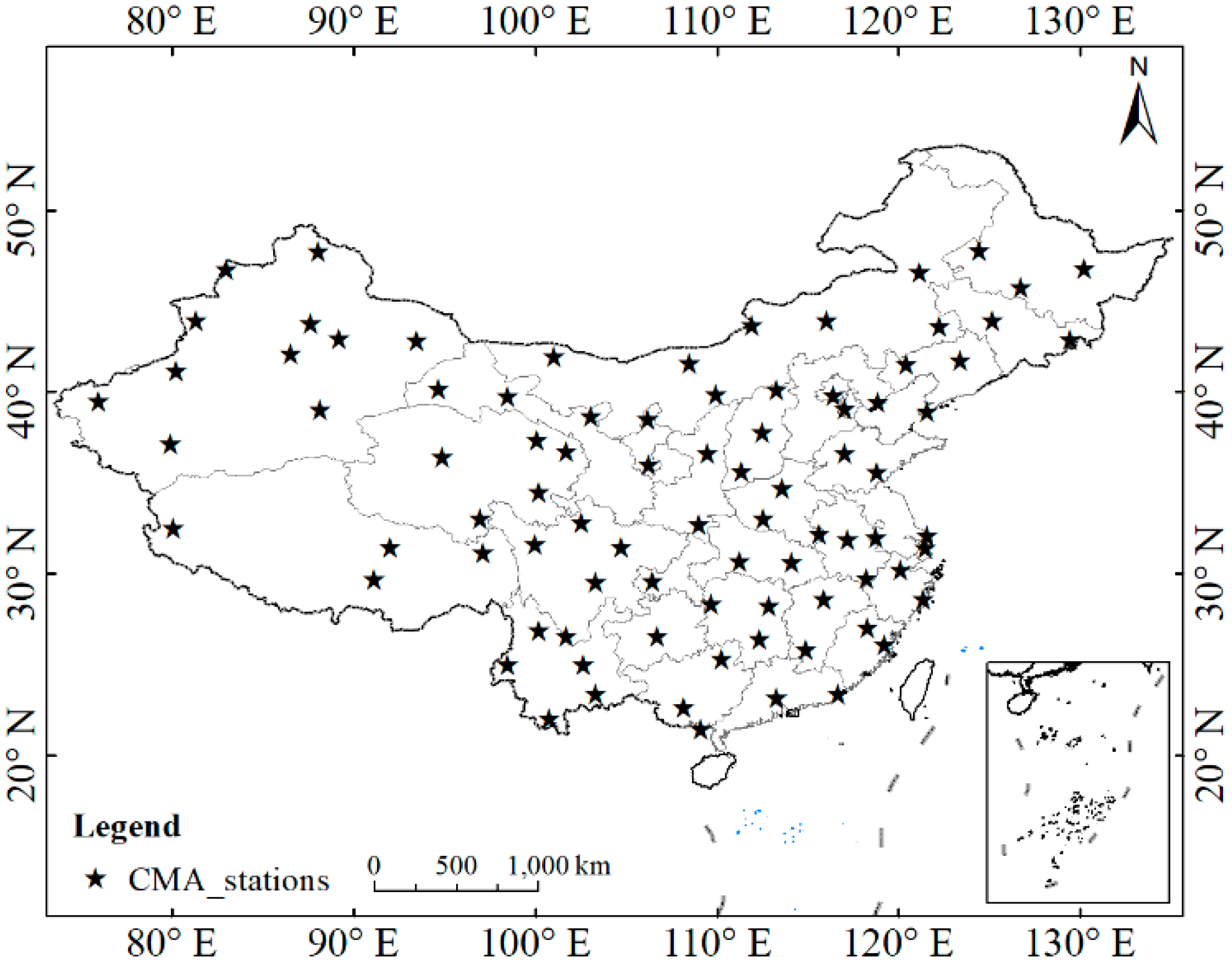
2.2. Ground Measurements
2.3. CERES–EBAF RS Data
3. Methodology
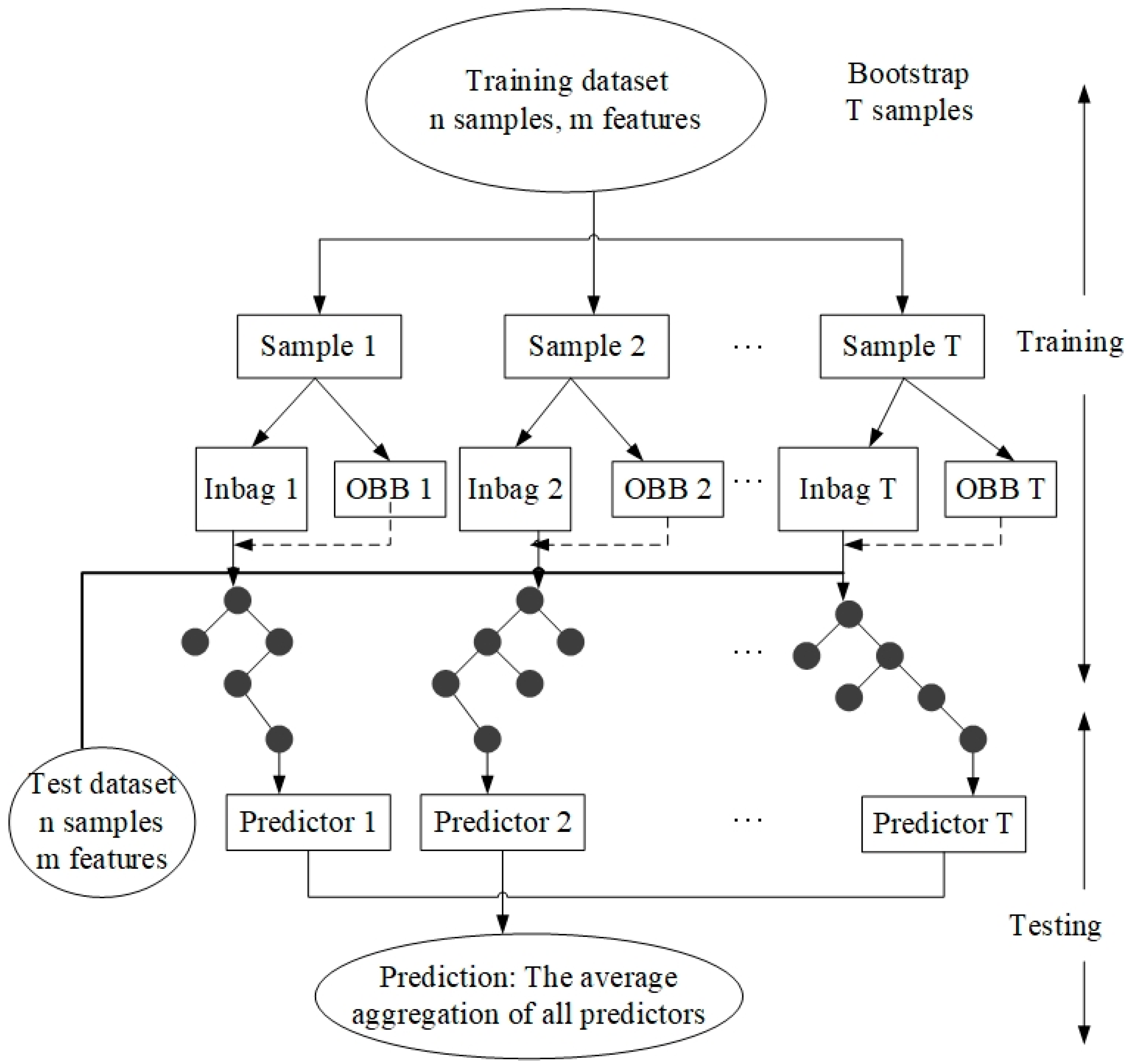
3.1. Random Forest
3.2. Model Construction
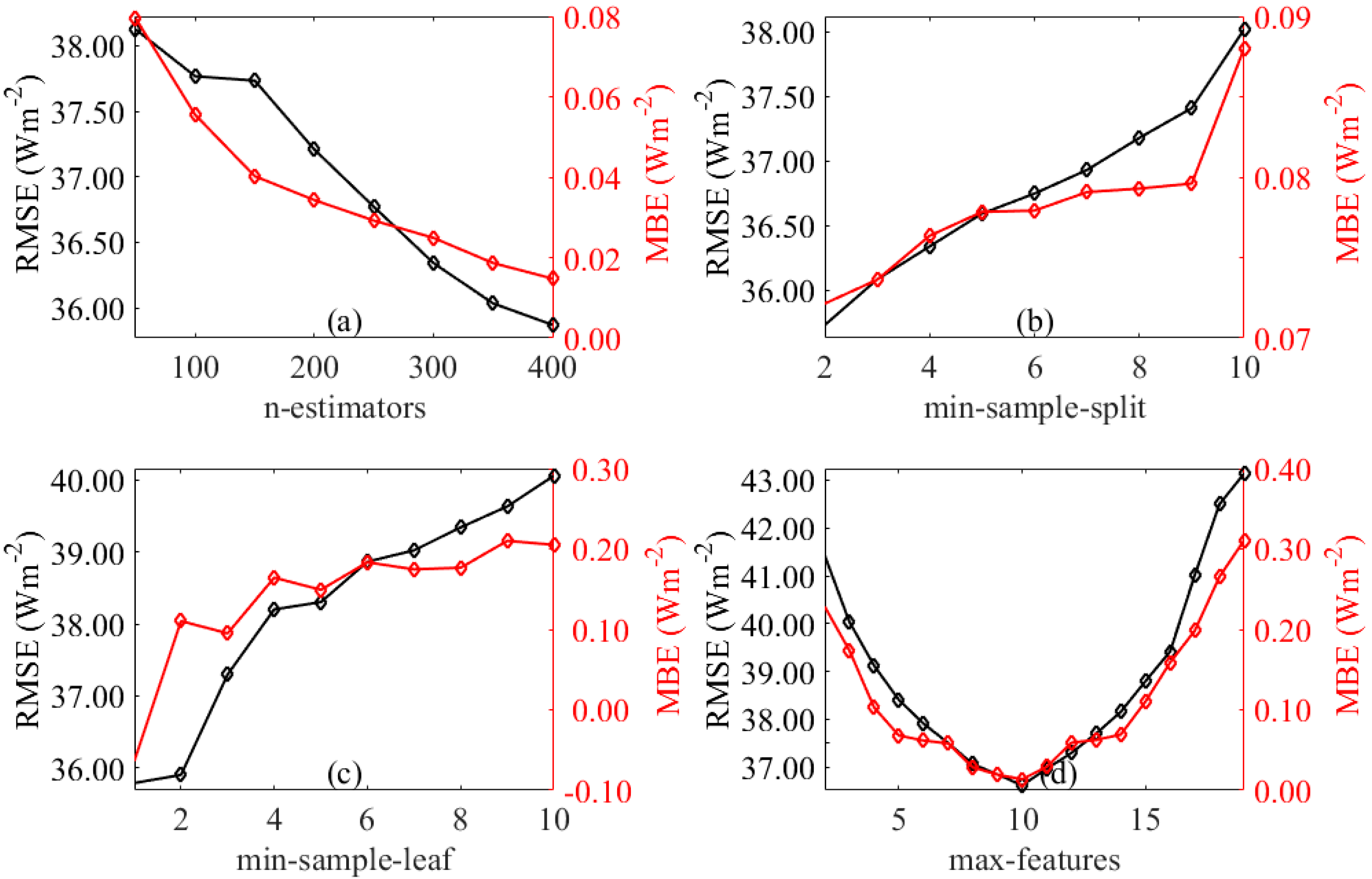
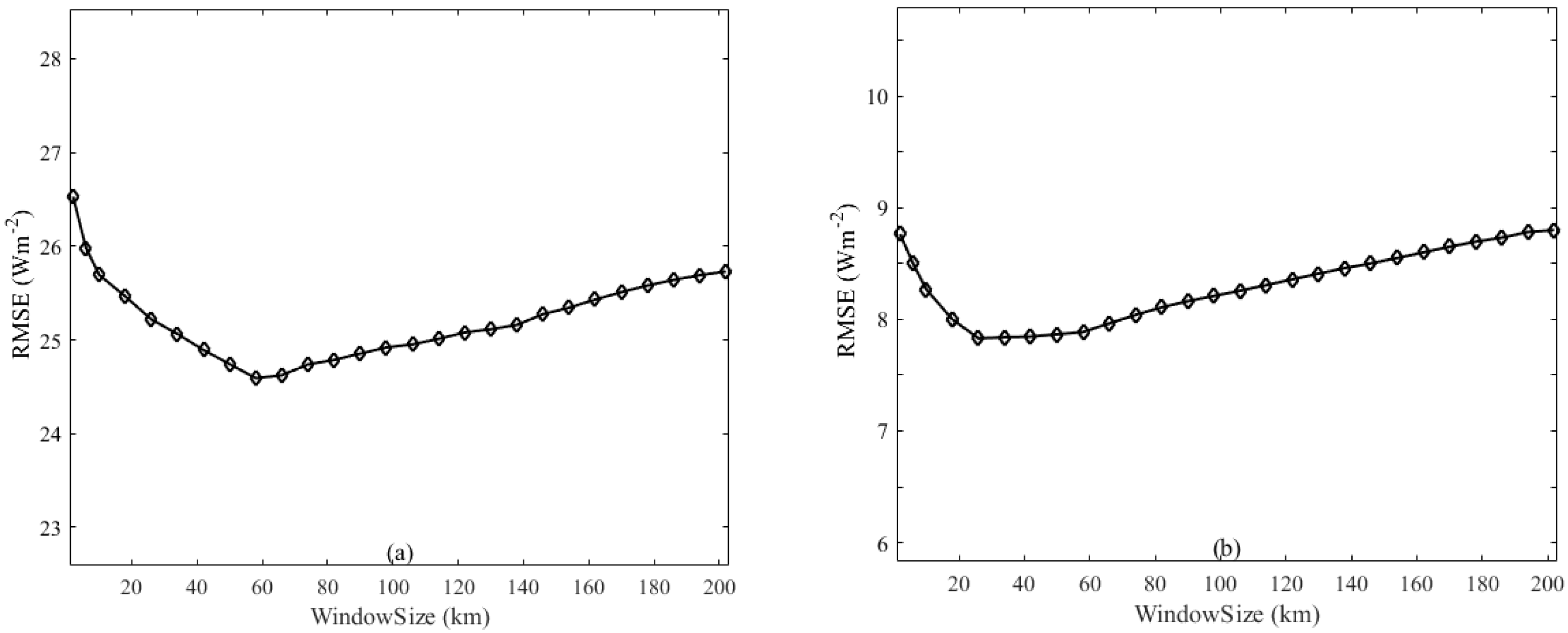
3.3. Sensitivity Analysis and Scaling Issue
4. Results and Analysis
4.1. Validation Against Ground Measurements
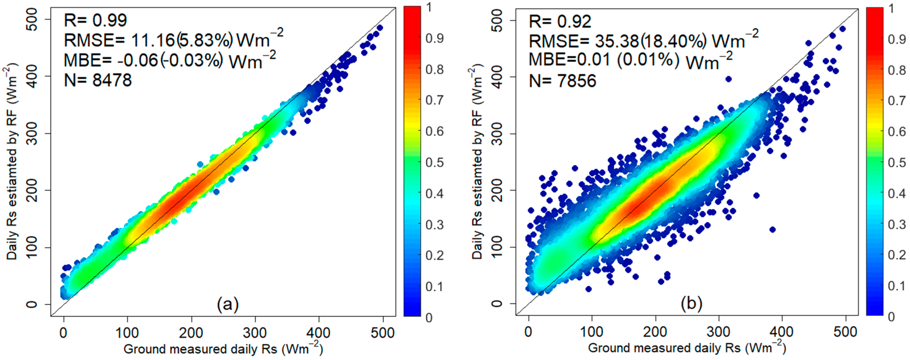
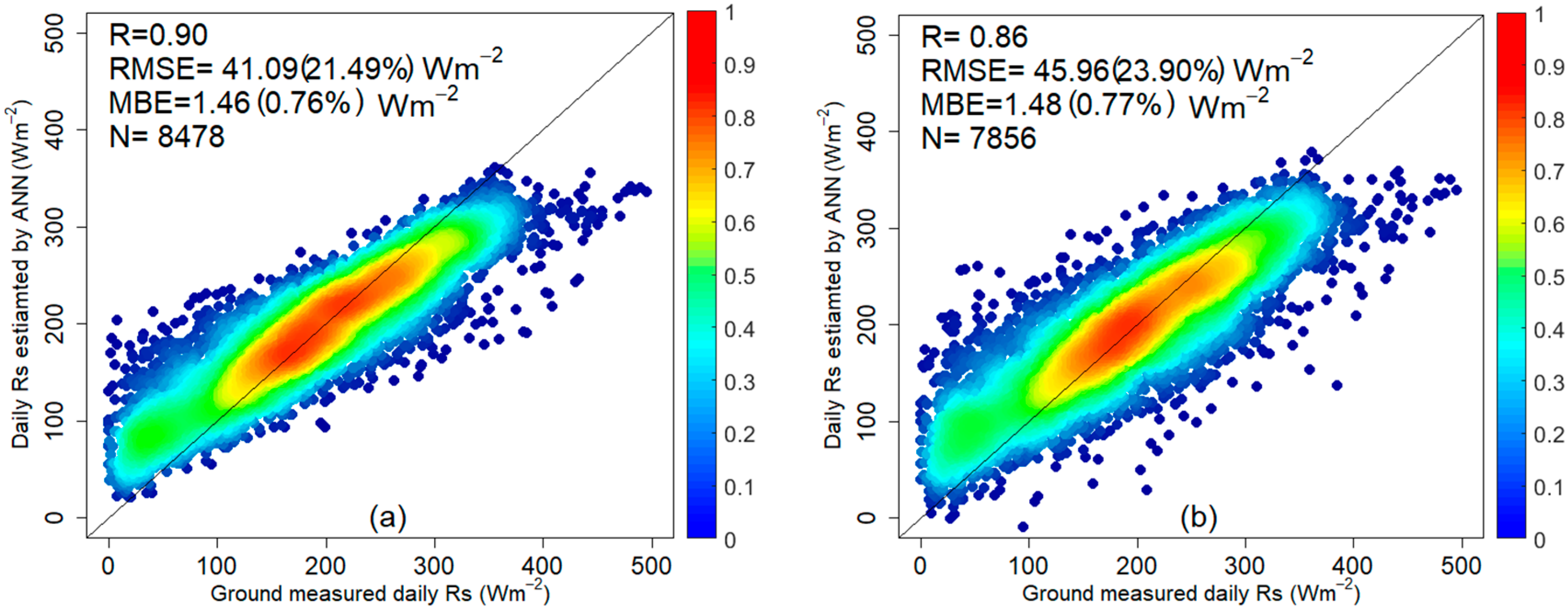
4.1.1. Validation at a Daily Time Scale
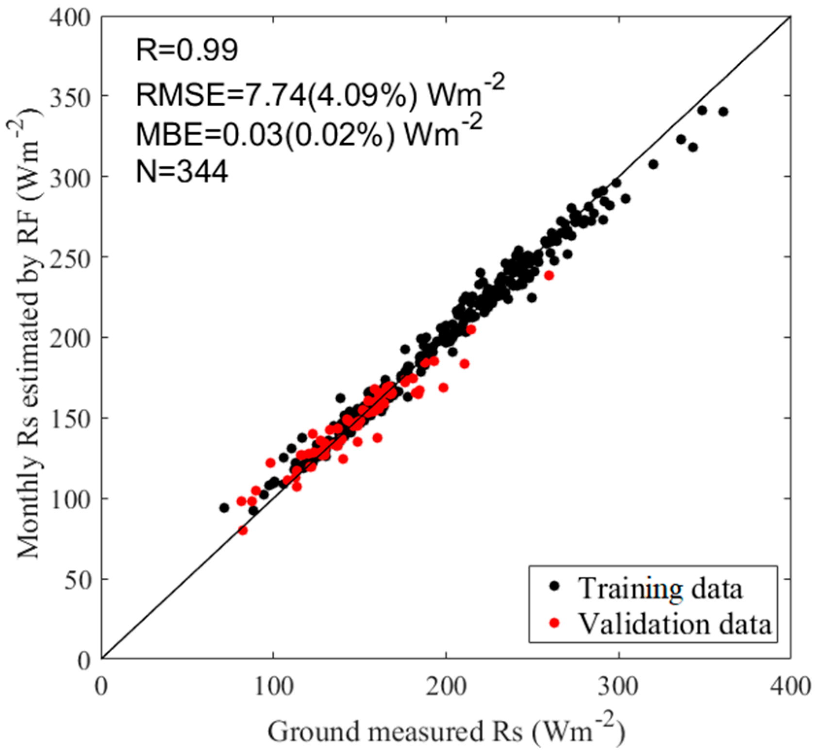
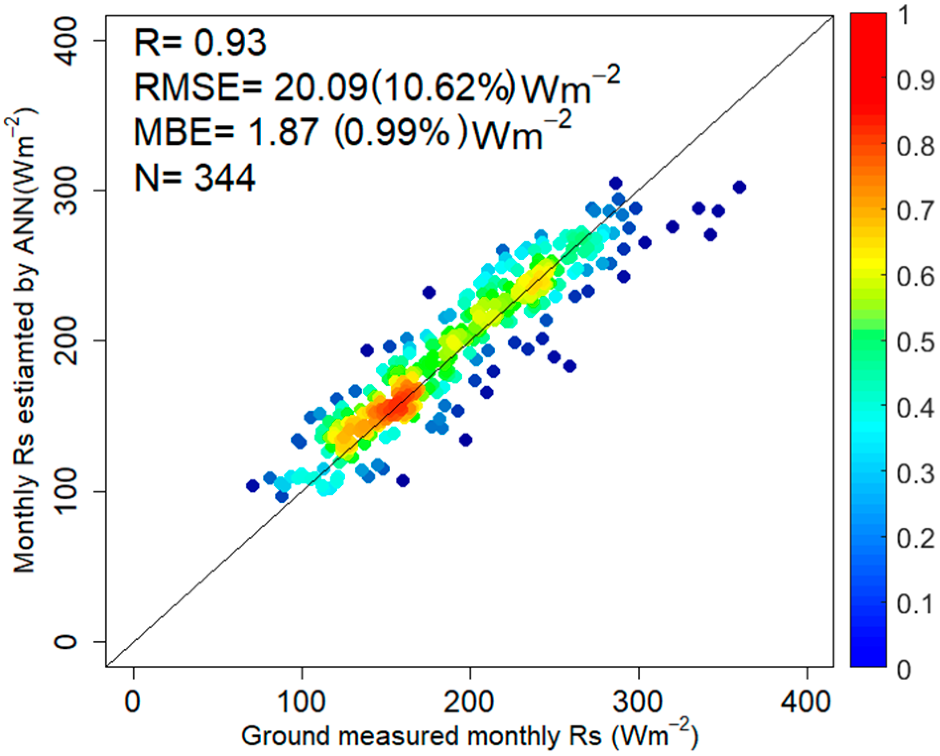
4.1.2. Validation at a Monthly Time Scale
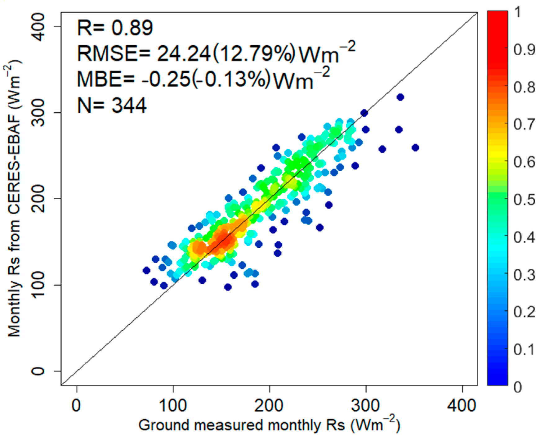
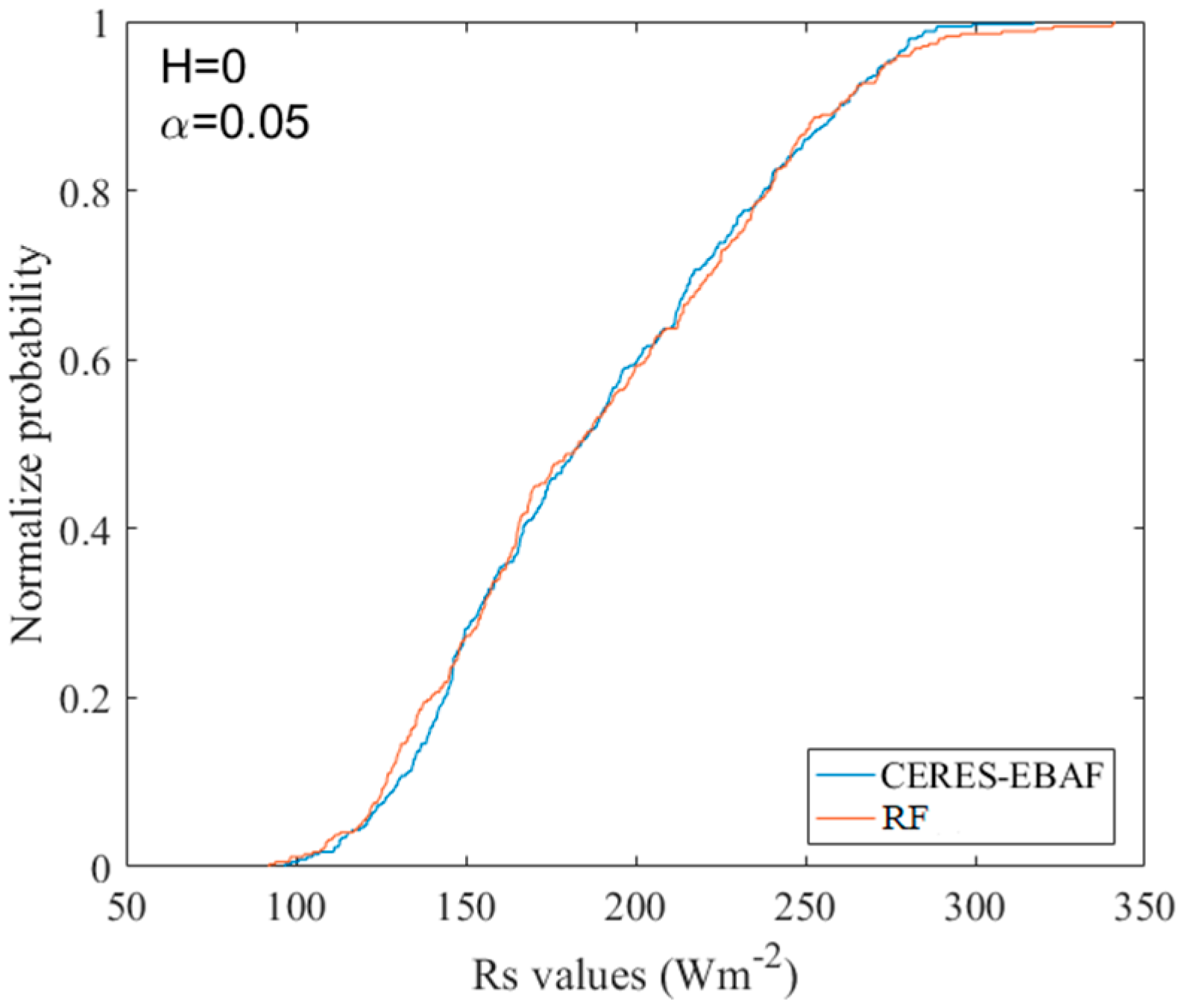
4.2. Comparison with CERES–EBAF
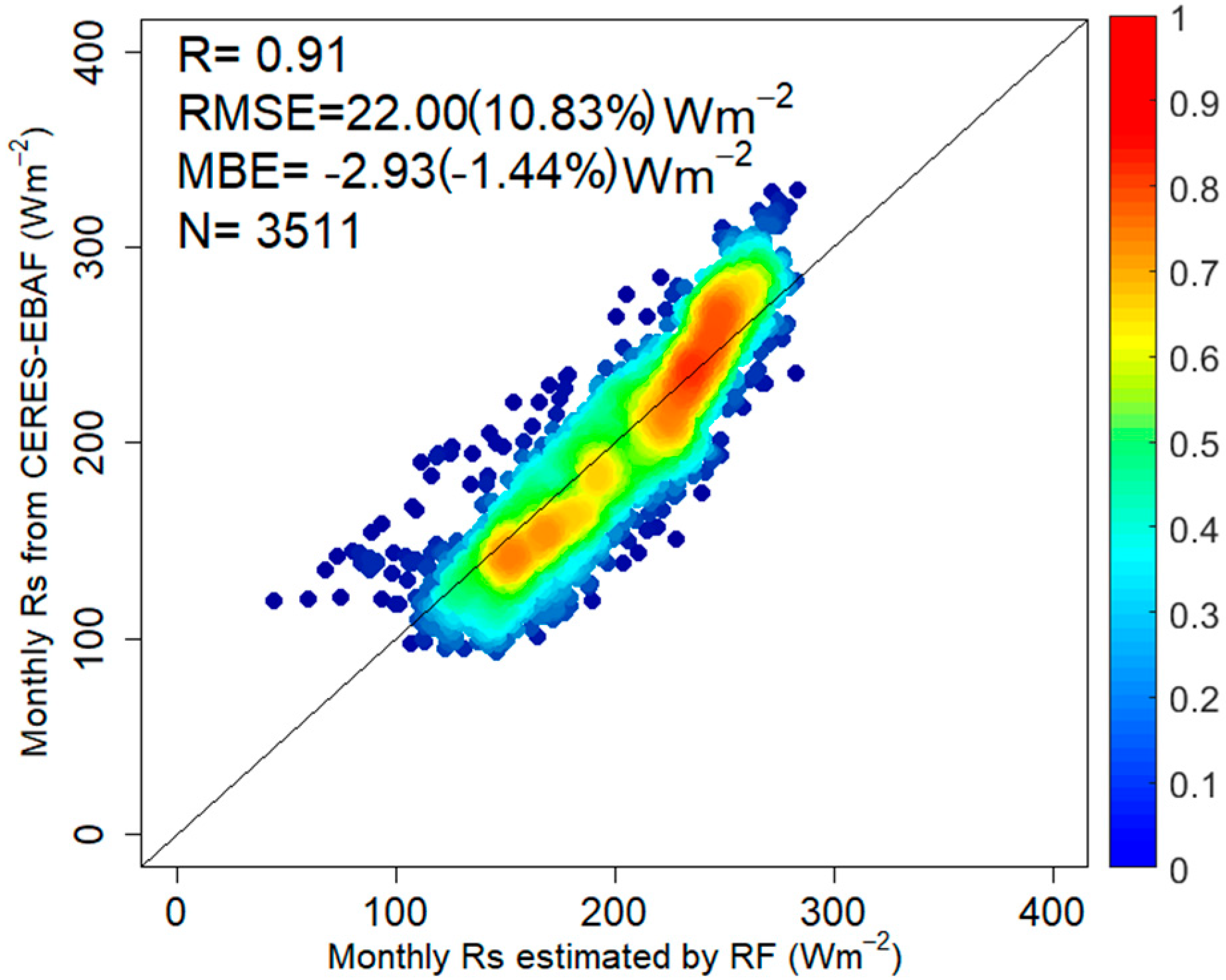
4.2.1. Validation Against Ground Measurements
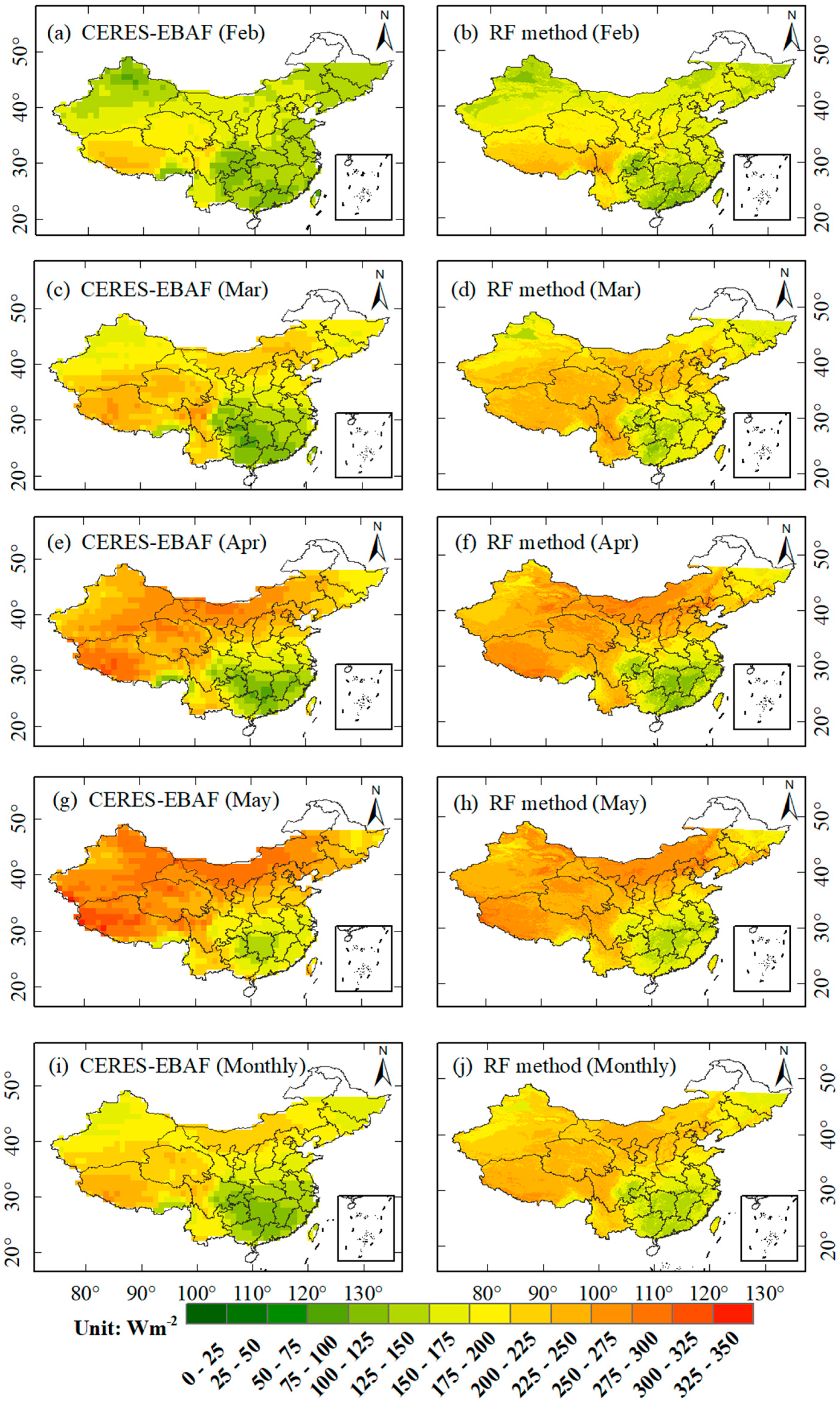
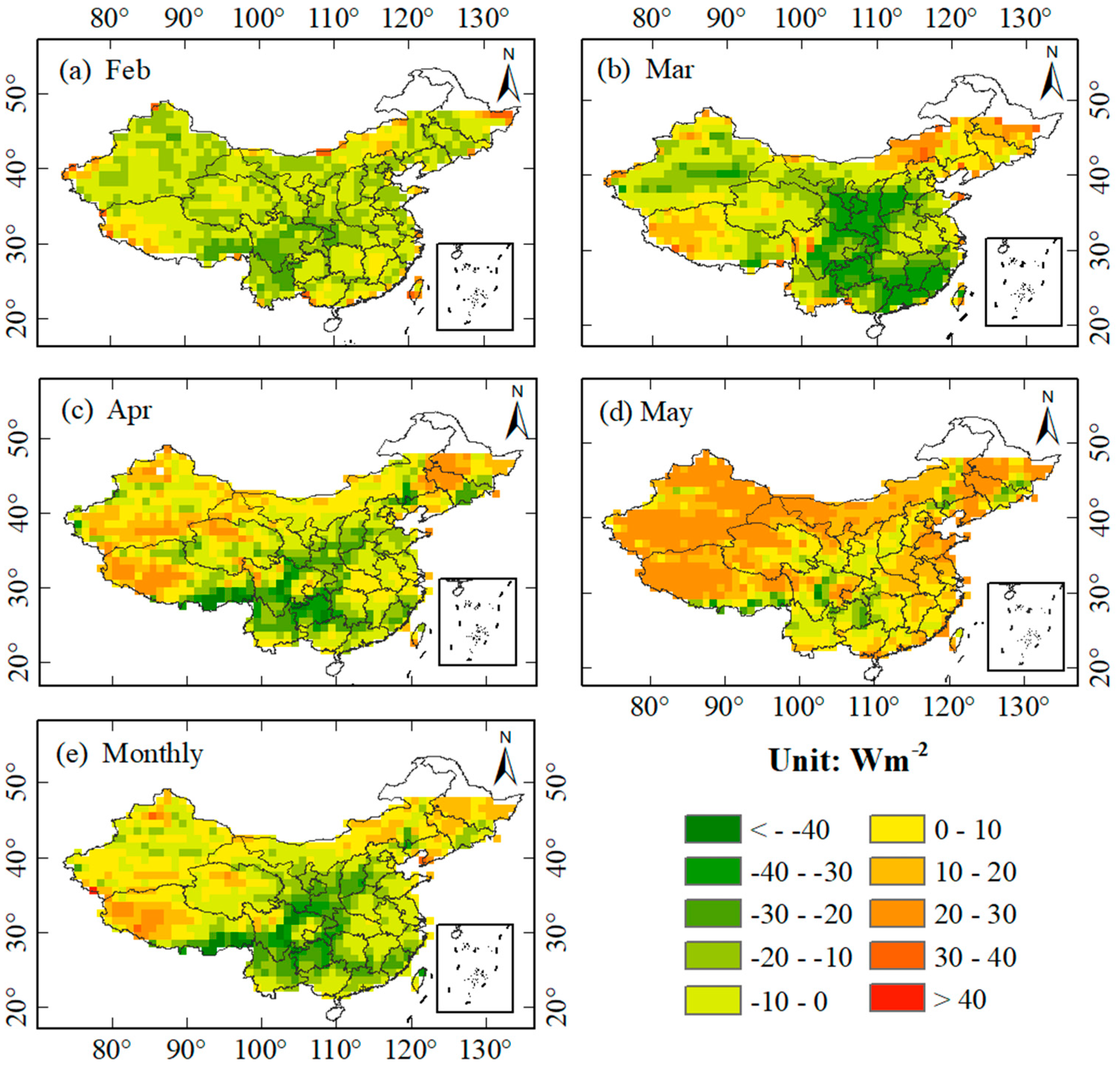
4.2.2. Mapping RS of China
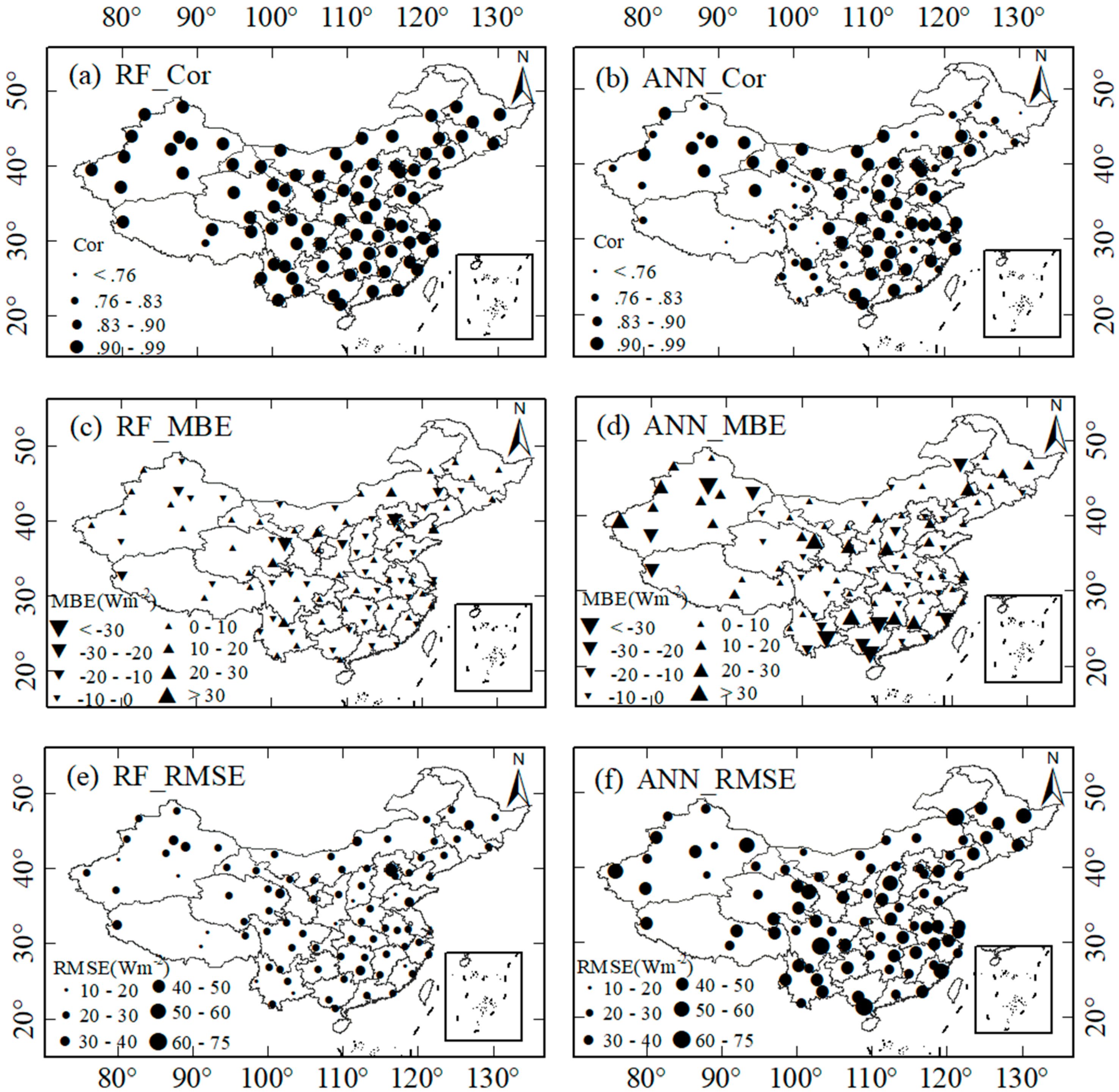
4.3. Comparison with ANN
5. Discussion
6. Conclusions
Author Contributions
Funding
Acknowledgments
Conflicts of Interest
References
- Gui, S.; Liang, S.; Wang, K.; Li, L.; Zhang, X. Assessment of three satellite-estimated land surface downwelling shortwave irradiance data sets. IEEE Geosci. Remote Sens. Lett. 2010, 7, 776–780. [Google Scholar] [CrossRef]
- Liang, S.; Wang, K.; Zhang, X.; Wild, M. Review on estimation of land surface radiation and energy budgets from ground measurement, remote sensing and model simulations. IEEE J. Sel. Top. Appl. Earth Obs. Remote Sens. 2010, 3, 225–240. [Google Scholar] [CrossRef]
- Ryu, Y.; Jiang, C.; Kobayashi, H.; Detto, M. MODIS-derived global land products of shortwave radiation and diffuse and total photosynthetically active radiation at 5 km resolution from 2000. Remote Sens. Environ. 2018, 204, 812–825. [Google Scholar] [CrossRef]
- Yang, K.; He, J.; Tang, W.; Qin, J.; Cheng, C.C.K. On downward shortwave and longwave radiations over high altitude regions: Observation and modeling in the Tibetan Plateau. Agric. For. Meteorol. 2010, 150, 38–46. [Google Scholar] [CrossRef]
- Singh, J.; Kumar, M. Solar radiation over four cities of India: Trend analysis using Mann-Kendall test. Int. J. Renew. Energy Res. 2016, 6, 1385–1395. [Google Scholar]
- Norris, J.R.; Wild, M. Trends in aerosol radiative effects over China and Japan inferred from observed cloud cover, solar “dimming,” and solar “brightening”. J. Geophys. Res. Atmos. 2009, 114. [Google Scholar] [CrossRef]
- Kambezidis, H.D.; Kaskaoutis, D.G.; Kharol, S.K.; Moorthy, K.K.; Satheesh, S.K.; Kalapureddy, M.C.R.; Badarinath, K.V.S.; Sharma, A.R.; Wild, M. Multi-decadal variation of the net downward shortwave radiation over south Asia: The solar dimming effect. Atmos. Environ. 2012, 50, 360–372. [Google Scholar] [CrossRef]
- Qian, Y.; Wang, W.; Leung, L.R.; Kaiser, D.P. Variability of solar radiation under cloud-free skies in China: The role of aerosols. Geophys. Res. Lett. 2007, 34. [Google Scholar] [CrossRef]
- Liang, S.L.; Zheng, T.; Liu, R.G.; Fang, H.L.; Tsay, S.C.; Running, S. Estimation of incident photosynthetically active radiation from Moderate Resolution Imaging Spectrometer data. J. Geophys. Res. Atmos. 2006, 111. [Google Scholar] [CrossRef] [Green Version]
- Zhang, X.; Liang, S.; Wild, M.; Jiang, B. Analysis of surface incident shortwave radiation from four satellite products. Remote Sens. Environ. 2015, 165, 186–202. [Google Scholar] [CrossRef]
- Liu, X.; Mei, X.; Li, Y.; Zhang, Y.; Wang, Q.; Jensen, J.R.; Porter, J.R. Calibration of the Ångström—Prescott coefficients (a, b) under different time scales and their impacts in estimating global solar radiation in the Yellow River basin. Agric. For. Meteorol. 2009, 149, 697–710. [Google Scholar] [CrossRef]
- Wang, J.; White, K.; Robinson, G.J. Estimating surface net solar radiation by use of Landsat-5 TM and digital elevation models. Int. J. Remote Sens. 2000, 21, 31–43. [Google Scholar] [CrossRef]
- Harries, J.E.; Russell, J.E.; Hanafin, J.A.; Brindley, H.; Futyan, J.; Rufus, J.; Kellock, S.; Matthews, G.; Wrigley, R.; Last, A.; et al. The geostationary earth radiation budget project. Bull. Am. Meteorol. Soc. 2005, 86, 945–960. [Google Scholar] [CrossRef] [Green Version]
- Shahi, N.R.; Agarwal, N.; Sharma, R.; Thapliyal, P.K.; Joshi, P.C.; Sarkar, A. Improved estimation of shortwave radiation over equatorial Indian Ocean using geostationary satellite data. IEEE Geosci. Remote Sens. Lett. 2010, 7, 563–566. [Google Scholar] [CrossRef]
- Zhang, X.; Liang, S.; Zhou, G.; Wu, H.; Zhao, X. Generating Global LAnd Surface Satellite incident shortwave radiation and photosynthetically active radiation products from multiple satellite data. Remote Sens. Environ. 2014, 152, 318–332. [Google Scholar] [CrossRef]
- Wang, K.; Zhou, X.; Liu, J.; Sparrow, M. Estimating surface solar radiation over complex terrain using moderate-resolution satellite sensor data. Int. J. Remote Sens. 2005, 26, 47–58. [Google Scholar] [CrossRef]
- Cess, R.D.; Dutton, E.G.; Deluisi, J.J.; Jiang, F. Determining surface solar absorption from broadband satellite measurements for clear skies: Comparison with surface measurements. J. Clim. 1991, 4, 236–247. [Google Scholar] [CrossRef] [Green Version]
- Tang, W.J.; Yang, K.; Sun, Z.; Qin, J.; Niu, X.L. Global performance of a fast parameterization scheme for estimating surface solar radiation from MODIS data. IEEE Trans. Geosci. Remote Sens. 2017, 55, 3558–3571. [Google Scholar] [CrossRef]
- Qin, J.; Tang, W.J.; Yang, K.; Lu, N.; Niu, X.L.; Liang, S.L. An efficient physically based parameterization to derive surface solar irradiance based on satellite atmospheric products. J. Geophys. Res. Atmos. 2015, 120, 4975–4988. [Google Scholar] [CrossRef]
- Mueller, R.W.; Matsoukas, C.; Gratzki, A.; Behr, H.D.; Hollmann, R. The CM-SAF operational scheme for the satellite based retrieval of solar surface irradiance—A LUT based eigenvector hybrid approach. Remote Sens. Environ. 2009, 113, 1012–1024. [Google Scholar] [CrossRef]
- Xia, S.; Mestas-Nuñez, A.; Xie, H.; Tang, J.; Vega, R. Characterizing variability of solar irradiance in San Antonio, Texas using satellite observations of cloudiness. Remote Sens. 2018, 10, 2016. [Google Scholar] [CrossRef] [Green Version]
- Chen, L.; Yan, G.; Wang, T.; Ren, H.; Hu, R.; Chen, S.; Zhou, H. Spatial scale consideration for estimating all-sky surface shortwave radiation with a modified 1-D radiative transfer model. IEEE J. Sel. Top. Appl. Earth Obs. Remote Sens. 2019, 12, 821–835. [Google Scholar] [CrossRef]
- Zhang, Y.; He, T.; Liang, S.; Wang, D.; Yu, Y. Estimation of all-sky instantaneous surface incident shortwave radiation from Moderate Resolution Imaging Spectroradiometer data using optimization method. Remote Sens. Environ. 2018, 209, 468–479. [Google Scholar] [CrossRef]
- Kato, S.; Loeb, N.G.; Rose, F.G.; Doelling, D.R.; Rutan, D.A.; Caldwell, T.E.; Yu, L.; Weller, R.A. Surface irradiances consistent with CERES-derived top-of-atmosphere shortwave and longwave irradiances. J. Clim. 2013, 26, 2719–2740. [Google Scholar] [CrossRef]
- Kato, S.; Rose, F.G.; Sun-Mack, S.; Miller, W.F.; Chen, Y.; Rutan, D.A.; Stephens, G.L.; Loeb, N.G.; Minnis, P.; Wielicki, B.A.; et al. Improvements of top-of-atmosphere and surface irradiance computations with CALIPSO-, CloudSat-, and MODIS-derived cloud and aerosol properties. J. Geophys. Res. Atmos. 2011, 116. [Google Scholar] [CrossRef]
- Romano, F.; Cimini, D.; Cersosimo, A.; Di Paola, F.; Gallucci, D.; Gentile, S.; Geraldi, E.; Larosa, S.; Nilo, S.T.; Ricciardelli, E.; et al. Improvement in surface solar irradiance estimation using HRV/MSG data. Remote Sens. 2018, 10, 1288. [Google Scholar] [CrossRef] [Green Version]
- Riihelä, A.; Kallio, V.; Devraj, S.; Sharma, A.; Lindfors, A. Validation of the SARAH-E satellite-based surface solar radiation estimates over India. Remote Sens. 2018, 10, 392. [Google Scholar] [CrossRef] [Green Version]
- Olpenda, A.; Stereńczak, K.; Będkowski, K. Modeling solar radiation in the forest using remote sensing data: A review of approaches and opportunities. Remote Sens. 2018, 10, 694. [Google Scholar] [CrossRef] [Green Version]
- Lee, S.-H.; Kim, B.-Y.; Lee, K.-T.; Zo, I.-S.; Jung, H.-S.; Rim, S.-H. Retrieval of reflected shortwave radiation at the top of the atmosphere using Himawari-8/AHI data. Remote Sens. 2018, 10, 213. [Google Scholar] [CrossRef] [Green Version]
- Ineichen, P. High turbidity solis clear sky model: Development and validation. Remote Sens. 2018, 10, 435. [Google Scholar] [CrossRef] [Green Version]
- Kambezidis, H.D.; Psiloglou, B.E.; Karagiannis, D.; Dumka, U.C.; Kaskaoutis, D.G. Meteorological Radiation Model (MRM v6.1): Improvements in diffuse radiation estimates and a new approach for implementation of cloud products. Renew. Sustain. Energy Rev. 2017, 74, 616–637. [Google Scholar] [CrossRef]
- Zhang, M.; Wang, Y.; Ma, Y.Y.; Wang, L.C.; Gong, W.; Liu, B.M. Spatial distribution and temporal variation of aerosol optical depth and radiative effect in South China and its adjacent area. Atmos. Environ. 2018, 188, 120–128. [Google Scholar] [CrossRef]
- Feng, F.; Wang, K. Determining factors of monthly to decadal variability in surface solar radiation in China: Evidences from current reanalyses. J. Geophys. Res. Atmos. 2019, 124, 9161–9182. [Google Scholar] [CrossRef] [Green Version]
- Deneke, H.M.; Feijt, A.J.; Roebeling, R.A. Estimating surface solar irradiance from METEOSAT SEVIRI-derived cloud properties. Remote Sens. Environ. 2008, 112, 3131–3141. [Google Scholar] [CrossRef]
- Levy, R.C.; Remer, L.A.; Kleidman, R.G.; Mattoo, S.; Ichoku, C.; Kahn, R.; Eck, T.F. Global evaluation of the Collection 5 MODIS dark-target aerosol products over land. Atmos. Chem. Phys. 2010, 10, 10399–10420. [Google Scholar] [CrossRef] [Green Version]
- Deo, R.C.; Şahin, M. Forecasting long-term global solar radiation with an ANN algorithm coupled with satellite-derived (MODIS) land surface temperature (LST) for regional locations in Queensland. Renew. Sustain. Energy Rev. 2017, 72, 828–848. [Google Scholar] [CrossRef]
- Wang, T.; Yan, G.; Chen, L. Consistent retrieval methods to estimate land surface shortwave and longwave radiative flux components under clear-sky conditions. Remote Sens. Environ. 2012, 124, 61–71. [Google Scholar] [CrossRef]
- Zhou, Q.T.; Flores, A.; Glenn, N.F.; Walters, R.; Hang, B.S. A machine learning approach to estimation of downward solar radiation from satellite-derived data products: An application over a semi-arid ecosystem in the US. PLoS ONE 2017, 12, e0180239. [Google Scholar] [CrossRef] [Green Version]
- Jiang, B.; Liang, S.; Ma, H.; Zhang, X.; Xiao, Z.; Zhao, X.; Jia, K.; Yao, Y.; Jia, A. GLASS daytime all-wave net radiation product: Algorithm development and preliminary validation. Remote Sens. 2016, 8, 222. [Google Scholar] [CrossRef] [Green Version]
- Yang, L.; Zhang, X.T.; Liang, S.L.; Yao, Y.J.; Jia, K.; Jia, A.L. Estimating surface downward shortwave radiation over China based on the gradient boosting decision tree method. Remote Sens. 2018, 10, 185. [Google Scholar] [CrossRef] [Green Version]
- Tang, W.J.; Qin, J.; Yang, K.; Liu, S.M.; Lu, N.; Niu, X.L. Retrieving high-resolution surface solar radiation with cloud parameters derived by combining MODIS and MTSAT data. Atmos. Chem. Phys. 2016, 16, 2543–2557. [Google Scholar] [CrossRef] [Green Version]
- Wei, Y.; Zhang, X.; Hou, N.; Zhang, W.; Jia, K.; Yao, Y. Estimation of surface downward shortwave radiation over China from AVHRR data based on four machine learning methods. Sol. Energy 2019, 177, 32–46. [Google Scholar] [CrossRef]
- Ghimire, S.; Deo, R.C.; Raj, N.; Mi, J. Wavelet-based 3-phase hybrid SVR model trained with satellite-derived predictors, particle swarm optimization and maximum overlap discrete wavelet transform for solar radiation prediction. Renew. Sustain. Energy Rev. 2019, 113, 109247. [Google Scholar] [CrossRef]
- Fan, J.; Wu, L.; Ma, X.; Zhou, H.; Zhang, F. Hybrid support vector machines with heuristic algorithms for prediction of daily diffuse solar radiation in air-polluted regions. Renew. Energy 2020, 145, 2034–2045. [Google Scholar] [CrossRef]
- Chen, F.; Zhou, Z.; Lin, A.; Niu, J.; Qin, W.; Yang, Z. Evaluation of direct horizontal irradiance in China using a physically-based model and machine learning methods. Energies 2019, 12, 150. [Google Scholar] [CrossRef] [Green Version]
- Hao, D.; Asrar, G.R.; Zeng, Y.; Zhu, Q.; Wen, J.; Xiao, Q.; Chen, M. Estimating hourly land surface downward shortwave and photosynthetically active radiation from DSCOVR/EPIC observations. Remote Sens. Environ. 2019, 232, 111320. [Google Scholar] [CrossRef]
- Belgiu, M.; Drăguţ, L. Random forest in remote sensing: A review of applications and future directions. ISPRS J. Photogramm. Remote Sens. 2016, 114, 24–31. [Google Scholar] [CrossRef]
- Kim, B.-Y.; Lee, K.-T.; Jee, J.-B.; Zo, I.-S. Retrieval of outgoing longwave radiation at top-of-atmosphere using Himawari-8 AHI data. Remote Sens. Environ. 2018, 204, 498–508. [Google Scholar] [CrossRef]
- Damiani, A.; Irie, H.; Horio, T.; Takamura, T.; Khatri, P.; Takenaka, H.; Nagao, T.; Nakajima, T.Y.; Cordero, R.R. Evaluation of Himawari-8 surface downwelling solar radiation by ground-based measurements. Atmos. Meas. Tech. 2018, 11, 2501–2521. [Google Scholar] [CrossRef] [Green Version]
- Bessho, K.; Date, K.; Hayashi, M.; Ikeda, A.; Imai, T.; Inoue, H.; Kumagai, Y.; Miyakawa, T.; Murata, H.; Ohno, T.; et al. An introduction to Himawari-8/9-Japan’s new-generation geostationary meteorological satellites. J. Meteorol. Soc. Jpn. 2016, 94, 151–183. [Google Scholar] [CrossRef] [Green Version]
- Frouin, R.; Murakami, H. Estimating photosynthetically available radiation at the ocean surface from ADEOS-II Global Imager data. J. Oceanogr. 2007, 63, 493–503. [Google Scholar] [CrossRef]
- Shi, H.; Li, W.; Fan, X.; Zhang, J.; Hu, B.; Husi, L.; Shang, H.; Han, X.; Song, Z.; Zhang, Y.; et al. First assessment of surface solar irradiance derived from Himawari-8 across China. Sol. Energy 2018, 174, 164–170. [Google Scholar] [CrossRef]
- Yu, Y.; Shi, J.; Wang, T.; Letu, H.; Yuan, P.; Zhou, W.; Hu, L. Evaluation of the Himawari-8 Shortwave Downward Radiation (SWDR) product and its comparison with the CERES-SYN, MERRA-2, and ERA-interim datasets. IEEE J. Sel. Top. Appl. Earth Obs. Remote Sens. 2018, 12, 519–532. [Google Scholar] [CrossRef]
- Sawada, Y.; Okamoto, K.; Kunii, M.; Miyoshi, T. Assimilating every-10-minute Himawari-8 infrared radiances to improve convective predictability. J. Geophys. Res. Atmos. 2019, 124, 2546–2561. [Google Scholar] [CrossRef]
- Schmit, T.J.; Griffith, P.; Gunshor, M.M.; Daniels, J.M.; Goodman, S.J.; Lebair, W.J. A closer look at the ABI on the GOES-R series. Bull. Am. Meteorol. Soc. 2016, 98, 681–698. [Google Scholar] [CrossRef]
- Zhang, W.; Xu, H.; Zheng, F. Aerosol optical depth retrieval over East Asia using Himawari-8/AHI data. Remote Sens. 2018, 10, 137. [Google Scholar] [CrossRef] [Green Version]
- Gelaro, R.; McCarty, W.; Suárez, M.J.; Todling, R.; Molod, A.; Takacs, L.; Randles, C.A.; Darmenov, A.; Bosilovich, M.G.; Reichle, R.; et al. The modern-era retrospective analysis for research and applications, Version 2 (MERRA-2). J. Clim. 2017, 30, 5419–5454. [Google Scholar] [CrossRef]
- Hinkelman, L.M. The global radiative energy budget in MERRA and MERRA-2: Evaluation with respect to CERES EBAF data. J. Clim. 2019, 32, 1973–1994. [Google Scholar] [CrossRef]
- Matuszko, D. Long-term variability in solar radiation in Krakow based on measurements of sunshine duration. Int. J. Climatol. 2014, 34, 228–234. [Google Scholar] [CrossRef]
- He, Y.; Wang, K.; Zhou, C.; Wild, M. A revisit of global dimming and brightening based on the sunshine duration. Geophys. Res. Lett. 2018, 45, 4281–4289. [Google Scholar] [CrossRef]
- Yang, K.; Koike, T.; Stackhouse, P.; Mikovitz, C.; Cox, S.J. An assessment of satellite surface radiation products for highlands with Tibet instrumental data. Geophys. Res. Lett. 2006, 33. [Google Scholar] [CrossRef] [Green Version]
- Moradi, I. Quality control of global solar radiation using sunshine duration hours. Energy 2009, 34, 1–6. [Google Scholar] [CrossRef]
- Tang, W.; Yang, K.; He, J.; Qin, J. Quality control and estimation of global solar radiation in China. Sol. Energy 2010, 84, 466–475. [Google Scholar] [CrossRef]
- Tang, W.J.; Yang, K.; Qin, J.; Cheng, C.C.K.; He, J. Solar radiation trend across China in recent decades: A revisit with quality-controlled data. Atmos. Chem. Phys. 2011, 11, 393–406. [Google Scholar] [CrossRef] [Green Version]
- Tang, W.J.; Qin, J.; Yang, K.; Niu, X.L.; Zhang, X.T.; Yu, Y.; Zhu, X.D. Reconstruction of daily photosynthetically active radiation and its trends over China. J. Geophys. Res. Atmos. 2013, 118, 13292–13302. [Google Scholar] [CrossRef]
- Loeb, N.G.; Wielicki, B.A.; Doelling, D.R.; Smith, G.L.; Keyes, D.F.; Kato, S.; Manalo-Smith, N.; Wong, T. Toward optimal closure of the earth’s top-of-atmosphere radiation budget. J. Clim. 2009, 22, 748–766. [Google Scholar] [CrossRef] [Green Version]
- Kato, S.; Rose, F.G.; Rutan, D.A.; Thorsen, T.J.; Loeb, N.G.; Doelling, D.R.; Huang, X.; Smith, W.L.; Su, W.; Ham, S.-H. Surface irradiances of edition 4.0 clouds and the earth’s radiant energy system (CERES) energy balanced and filled (EBAF) data product. J. Clim. 2018, 31, 4501–4527. [Google Scholar] [CrossRef]
- Su, W.; Corbett, J.; Eitzen, Z.; Liang, L. Next-generation angular distribution models for top-of-atmosphere radiative flux calculation from CERES instruments: Methodology. Atmos. Meas. Tech. 2015, 8, 1467. [Google Scholar] [CrossRef] [Green Version]
- Loeb, N.G.; Doelling, D.R.; Wang, H.; Su, W.; Nguyen, C.; Corbett, J.G.; Liang, L.; Mitrescu, C.; Rose, F.G.; Kato, S. Clouds and the earth’s radiant energy system (CERES) energy balanced and filled (EBAF) top-of-atmosphere (TOA) edition-4.0 data product. J. Clim. 2018, 31, 895–918. [Google Scholar] [CrossRef]
- Ma, Q.; Wang, K.; Wild, M. Impact of geolocations of validation data on the evaluation of surface incident shortwave radiation from Earth System Models. J. Geophys. Res. Atmos. 2015, 120, 6825–6844. [Google Scholar] [CrossRef] [Green Version]
- Loeb, N. The Climate Data Guide: CERES EBAF: Clouds and Earth’s Radiant Energy Systems (CERES) Energy Balanced and Filled (EBAF). Available online: https://climatedataguide.ucar.edu/climate-data/ceres-ebaf-clouds-and-earths-radiant-energy-systems-ceres-energybalanced-and-filled (accessed on 1 February 2019).
- Breiman, L. Random forests. Mach. Learn. 2001, 45, 5–32. [Google Scholar] [CrossRef] [Green Version]
- Yu, P.S.; Yang, T.C.; Chen, S.Y.; Kuo, C.M.; Tseng, H.W. Comparison of random forests and support vector machine for real-time radar-derived rainfall forecasting. J. Hydrol. 2017, 552, 92–104. [Google Scholar] [CrossRef]
- Zamo, M.; Mestre, O.; Arbogast, P.; Pannekoucke, O. A benchmark of statistical regression methods for short-term forecasting of photovoltaic electricity production. Part II: Probabilistic forecast of daily production. Sol. Energy 2014, 105, 804–816. [Google Scholar] [CrossRef]
- Prasad, A.M.; Iverson, L.R.; Liaw, A. Newer classification and regression tree techniques: Bagging and random forests for ecological prediction. Ecosystems 2006, 9, 181–199. [Google Scholar] [CrossRef]
- Verbyla, D.L. Classification trees—A new discrimination tool. Can. J. For. Res. 1987, 17, 1150–1152. [Google Scholar] [CrossRef]
- Gislason, P.O.; Benediktsson, J.A.; Sveinsson, J.R. Random Forests for land cover classification. Pattern Recognit. Lett. 2006, 27, 294–300. [Google Scholar] [CrossRef]
- Pedregosa, F.; Varoquaux, G.; Gramfort, A.; Michel, V.; Thirion, B.; Grisel, O.; Blondel, M.; Prettenhofer, P.; Weiss, R.; Dubourg, V.; et al. Scikit-learn: Machine learning in Python. J. Mach. Learn. Res. 2012, 12, 2825–2830. [Google Scholar]
- Ibrahim, I.A.; Khatib, T. A novel hybrid model for hourly global solar radiation prediction using random forests technique and firefly algorithm. Energy Convers. Manag. 2017, 138, 413–425. [Google Scholar] [CrossRef]
- Qu, Z.; Gschwind, B.; Lefevre, M.; Wald, L. Improving HelioClim-3 estimates of surface solar irradiance using the McClear clear-sky model and recent advances in atmosphere composition. Atmos. Meas. Tech. 2014, 7, 3927–3933. [Google Scholar] [CrossRef] [Green Version]
- Psiloglou, B.E.; Kambezidis, H.D.; Kaskaoutis, D.G.; Karagiannis, D.; Polo, J.M. Comparison between MRM simulations, CAMS and PVGIS databases with measured solar radiation components at the Methoni station, Greece. Renew. Energy 2020, 146, 1372–1391. [Google Scholar] [CrossRef]
- Linares-Rodriguez, A.; Ruiz-Arias, J.A.; Pozo-Vazquez, D.; Tovar-Pescador, J. An artificial neural network ensemble model for estimating global solar radiation from Meteosat satellite images. Energy 2013, 61, 636–645. [Google Scholar] [CrossRef]
- Massey, F.J. The Kolmogorov-Smirnov test for goodness of fit. J. Am. Stat. Assoc. 1951, 46, 68–78. [Google Scholar] [CrossRef]
- Meenal, R.; Selvakumar, A.I. Assessment of SVM, empirical and ANN based solar radiation prediction models with most influencing input parameters. Renew. Energy 2018, 121, 324–343. [Google Scholar] [CrossRef]
- Albrecht, B.A. Aerosols, cloud microphysics, and fractional cloudiness. Science 1989, 245, 1227–1230. [Google Scholar] [CrossRef] [PubMed]
- Hatzianastassiou, N.; Matsoukas, C.; Fotiadi, A.; Pavlakis, K.G.; Drakakis, E.; Hatzidimitriou, D.; Vardavas, I. Global distribution of Earth’s surface shortwave radiation budget. Atmos. Chem. Phys. 2005, 5, 2847–2867. [Google Scholar] [CrossRef] [Green Version]
- Yu, R.C.; Yu, Y.Q.; Zhang, M.H. Comparing cloud radiative properties between the eastern China and the Indian monsoon region. Adv. Atmos. Sci. 2001, 18, 1090–1102. [Google Scholar]
- Li, Z.; Lau, W.K.M.; Ramanathan, V.; Wu, G.; Ding, Y.; Manoj, M.G.; Liu, J.; Qian, Y.; Li, J.; Zhou, T.; et al. Aerosol and monsoon climate interactions over Asia. Rev. Geophys. 2016, 54, 866–929. [Google Scholar] [CrossRef]
- Wang, K.; Ma, Q.; Wang, X.; Wild, M. Urban impacts on mean and trend of surface incident solar radiation. Geophys. Res. Lett. 2014, 41, 4664–4668. [Google Scholar] [CrossRef] [Green Version]
- Johnson, R.; Zhang, T. Learning nonlinear functions using regularized greedy forest. IEEE Trans. Pattern Anal. Mach. Intell. 2014, 36, 942–954. [Google Scholar] [CrossRef] [Green Version]
- Salles, T.; Goncalves, M.; Rodrigues, V.; Rocha, L. Improving random forests by neighborhood projection for effective text classification. Inf. Syst. 2018, 77, 1–21. [Google Scholar] [CrossRef]
- Hagiwara, K.; Fukumizu, K. Relation between weight size and degree of over-fitting in neural network regression. Neural Netw. 2008, 21, 48–58. [Google Scholar] [CrossRef] [PubMed]


| Band | Descriptive Name | Central Wavelength (μm) | Spatial Resolution (km) | Primary Purpose |
|---|---|---|---|---|
| 1 | Blue | 0.46 | 1.0 | Daytime aerosol over land, coastal water mapping |
| 2 | Green | 0.51 | 1.0 | Green band-to produce color composite imagery |
| 3 | Red | 0.65 | 0.5 | Day time vegetation/burn scar and aerosols over water, winds |
| 4 | Vegetation | 0.86 | 1.0 | Daytime cirrus cloud |
| 5 | Snow/ice | 1.61 | 2.0 | Daytime cloud-top phase and particle size, snow |
| 6 | Cloud particle size | 2.26 | 2.0 | Daytime land/cloud properties, particle size, vegetation, snow |
| 7 | Shortwave window | 3.85 | 2.0 | Surface and cloud, fog at night, fire, and winds |
| 8 | Upper-level water vapor | 6.25 | 2.0 | High-level atmospheric water vapor, winds, and rainfall |
| 9 | Mid-level water vapor | 6.95 | 2.0 | Mid-level atmospheric water vapor, winds, and rainfall |
| 10 | Lower-level/Mid-level water vapor | 7.35 | 2.0 | Lower-level atmospheric water vapor, winds, and SO2 |
| 11 | Cloud-top phase | 8.60 | 2.0 | Total water for stability, cloud phase, dust, SO2, and rainfall |
| 12 | O3 | 9.63 | 2.0 | Total ozone, turbulence, and winds |
| 13 | Clean longwave window | 10.45 | 2.0 | Surface and cloud |
| 14 | Longwave window | 11.20 | 2.0 | Imagery, sea surface temperature, clouds, and rainfall |
| 15 | Dirty longwave window | 12.35 | 2.0 | Total water, ash, and sea surface temperature |
| 16 | CO2 | 13.30 | 2.0 | Air temperature, cloud heights and amounts |
| Parameters | Threshold | Intervals |
|---|---|---|
| n-estimators | 50–400 | 50 |
| max-features | 2–19 | 1 |
| min-samples-split | 2–10 | 1 |
| min-samples-leaf | 1–10 | 1 |
| Time Scale | Data | Method | R | RMSE (Wm−2) | MBE (Wm−2) |
|---|---|---|---|---|---|
| Daily | Training Data | RF | 0.99 | 11.16 (5.83%) | −0.06 (−0.03%) |
| ANN | 0.90 | 41.09 (21.49%) | 1.46 (0.76%) | ||
| Validation Data | RF | 0.92 | 35.38 (18.40%) | 0.01 (0.01%) | |
| ANN | 0.86 | 45.96 (23.90%) | 1.48 (0.77%) | ||
| Monthly | All Data | RF | 0.99 | 7.74 (4.09%) | 0.03 (0.02%) |
| ANN | 0.93 | 20.09 (10.62%) | 1.81 (0.99%) |
© 2020 by the authors. Licensee MDPI, Basel, Switzerland. This article is an open access article distributed under the terms and conditions of the Creative Commons Attribution (CC BY) license (http://creativecommons.org/licenses/by/4.0/).
Share and Cite
Hou, N.; Zhang, X.; Zhang, W.; Wei, Y.; Jia, K.; Yao, Y.; Jiang, B.; Cheng, J. Estimation of Surface Downward Shortwave Radiation over China from Himawari-8 AHI Data Based on Random Forest. Remote Sens. 2020, 12, 181. https://0-doi-org.brum.beds.ac.uk/10.3390/rs12010181
Hou N, Zhang X, Zhang W, Wei Y, Jia K, Yao Y, Jiang B, Cheng J. Estimation of Surface Downward Shortwave Radiation over China from Himawari-8 AHI Data Based on Random Forest. Remote Sensing. 2020; 12(1):181. https://0-doi-org.brum.beds.ac.uk/10.3390/rs12010181
Chicago/Turabian StyleHou, Ning, Xiaotong Zhang, Weiyu Zhang, Yu Wei, Kun Jia, Yunjun Yao, Bo Jiang, and Jie Cheng. 2020. "Estimation of Surface Downward Shortwave Radiation over China from Himawari-8 AHI Data Based on Random Forest" Remote Sensing 12, no. 1: 181. https://0-doi-org.brum.beds.ac.uk/10.3390/rs12010181