Monitoring Surface Soil Moisture Content over the Vegetated Area by Integrating Optical and SAR Satellite Observations in the Permafrost Region of Tibetan Plateau

Abstract

Surface soil moisture (SSM), the average water content of surface soil (up to 5 cm depth), plays a key role in the energy exchange within the ecosystem. We estimated SSM in areas with vegetation cover (grassland) by combining microwave and optical satellite measurements in the central Tibetan Plateau (TP) in 2015. We exploited TERRA moderate resolution imaging spectroradiometer (MODIS) and Sentinel-1A synthetic aperture radar (SAR) observations to estimate SSM through a simplified water-cloud model (sWCM). This model considers the impact of vegetation water content (VWC) to SSM retrieval by integrating the vegetation index (VI), the normalized difference water index (NDWI), or the normalized difference infrared index (NDII). Sentinel-1 SAR C-band backscattering coefficients, incidence angle, and NDWI/NDII were assimilated in the sWCM to monitor SSM. The soil moisture and temperature monitoring network on the central TP (CTP-SMTMN) measures SSM within the study area, and ground measurements were applied to train and validate the model. Via the proposed methods, we estimated the SSM in vegetated area with an R² of 0.43 and a ubRMSE of 0.06 m³/m³ when integrating the NDWI and with an R² of 0.45 and a ubRMSE of 0.06 m³/m³ when integrating the NDII.

1. Introduction

Soil moisture (SM) plays a key role in evapotranspiration as well as the water dynamics and energy transfer between land and the atmosphere [1,2,3,4,5,6,7]. SM has been assimilated in various land surface models (LSM) and atmospheric models to predict weather, drought, flood, and climate trends [6,8,9]. Understanding the spatial and temporal distribution of SM can therefore help us better analyze the regional and global water dynamics and improve the hydrology related models. Root zone SM (RZSM), defined as the SM at a depth from 0.5 to 1 m, is crucial for crop production and serves as an indicator for crop yield estimation [10,11]. However, RZSM cannot be monitored through satellite techniques currently. In contrast, surface soil moisture (SSM) is defined as the SM up to a depth of 5 cm and represents the interface between land and the atmosphere [5,6,7,8], various methods have been proposed to estimate SSM using satellite observations. We applied satellite measurements in this study to monitor SSM over the central of Tibetan Plateau (TP), since SSM plays a key role in regulating the energy and water transfer between land and atmosphere and has a significant impact on the regional climate of TP.

The cosmic-ray soil moisture observing system (COSMOS) allows to directly measure SM at various depths [12]. However, such point-based measurements do not fully reflect the overall situation, since SM shows a high spatial and temporal heterogeneity [6,9,12]. To overcome this limitation, remote sensing techniques have been used to provide spatial and temporal continuous land surface observation and are widely applied in SSM monitoring [6,9]. Currently, optical, thermal, and microwave methods are available [6,9].

When SM increases, the reflectance decreases inversely for solar band with wavelength from 0.4 to 2.5 μm. That is to say, surface soil with high water content is darker. This is the physical principle for estimating SSM with optical methods [6,9]. Various experiments and approaches have been conducted to describe the relationship between surface soil reflectance and its water content [13,14,15]. The thermal methods depend on the change of soil surface temperature with different SSM. Thermal inertia method only considers thermal bands, temperature/ vegetation index method analyzes solar reflective bands and thermal emissive bands together [9,16,17]. However, both optical and thermal bands are affected by weather conditions, cannot be used when there is a cloud cover. For instance, the 16-day revisit cycle of Landsat 8 makes it difficult to collect enough valuable observations within a specific study period. And, the optical/ thermal bands have limited penetration, they are therefore only feasible within bare soil under clear sky. However, monitoring SSM in a vegetated area is of great importance, since SSM is an important parameter for agricultural drought monitoring and has been widely applied in many LSM over vegetated areas.

In contrast, microwave techniques can be used under any weather condition using the electromagnetic radiation in the microwave region (0.5–100 cm) [6,9,18]. Both passive and active microwave sensors have been widely applied to monitor SSM [6,9,18]. Passive microwave sensors collect signals emitted by soil, while active microwave sensors send a pulse and analyze the soil reflected signal. Previous research works have shown that passive microwave sensors can be used to monitor global SSM through measuring the intensity of microwave emissivity from the soil [19,20,21,22]. Currently used passive microwave sensors for SSM measurements include the scanning multi-channel microwave radiometer (SMMR), the special sensor microwave imager (SSM/I), the advanced microwave scanning radiometer for EOS (AMSR-E), soil moisture and ocean salinity (SMOS), and soil moisture active passive (SMAP) [9,19,20,21,22]. Although showing a good temporal resolution (1–2 day), the main limitation of passive microwave methods is the coarse spatial resolution (10–35 km), making them unsuitable for applications at the fine scale.

Great progress has been made in mapping regional soil moisture with active microwave sensors, a microwave pulse that is sensitive to SM is sent and received [6,11]. SSM is estimated based on the difference between sent and received signals [23]. The active microwave remote sensing approaches such as synthetic aperture radar (SAR) with fine spatial resolutions (5–30 m), enable SSM monitoring at finer spatial scales. The SAR monitors SSM with three microwave bands: X-band (~3 cm), C-band (~6 cm), and L-band (~24 cm). Of these, the L-band has the strongest penetration, while X-band has the weakest penetration [4,24,25]. Microwave signals with longer wavelengths as L-band can penetrate the canopy and are reflected by the soil surface [4]. Currently, there are some SAR systems which are suitable for SM retrieval: the European remote-sensing satellite (ERS)-1/2/3 C-band, RADARSAR-1/2 C-band, advanced land observation satellite (ALOS), the phased array type L-band synthetic aperture radar (PALSAR), TerraSAT X-band (TSX), Sentinel-1/2/3 C-band (5.404 GHz) [26,27,28,29,30]. In this study, we used the Sentinel-1A SAR with moderate penetration of the C-band signal for the grassland area.

In the past few decades, SAR has been widely used to monitor SSM [28,31,32,33,34,35,36,37,38,39,40,41,42,43,44,45,46,47,48,49]. There is a strong relationship between the C-band backscattering coefficient and SSM, making the C-band backscattering coefficient and effective tool to estimate SSM. However, the relationship between backscattering coefficients and SSM varies significantly under different surface types and vegetation features [31,32,33,34,35,36,38,39,43,44,45,46,47,48,49]. Artificial neural network (ANN) and support vector machine (SVM) have been combined with regression algorithms to retrieve vegetated SSM [31,32,33,34,35]. Because of the concerns about vegetation characteristics, some vegetation backscattering models have been established to describe the contribution of vegetation, with the most widely used on being the water-cloud model (WCM). Based on the radiative transfer theory, the contribution of vegetation was modeled by considering both the volume scattering produced by vegetation and the attenuation effect of soil under vegetation on the backscattering. The total backscattering of the of the vegetated surface was derived from the backscattering of bare surface using the WCM [31,32,33,34,35,36,38,39,43,44,45,46,47,48,49]. The model simulated the backscattering of vegetated surfaces as a function of soil backscattering and the vegetation water content (VWC) [31,32,33,34,35,36,37,38,39,40,41,42,43,44,45,46,47,48,49].

Wang et al. integrated the advanced integral equation model (AIEM) with WCM to estimate SSM over vegetated area. However, it is still under debate which vegetation parameter is the most suitable one to estimate vegetation canopy backscattering in the WCM model. One of the major factors that affect the canopy backscattering is the VWC [40,41,42,44,45,48]. Several vegetation indices (VI) have been successfully applied to retrieve canopy VWC for grassland and agricultural areas [49,50,51,52,53,54]. 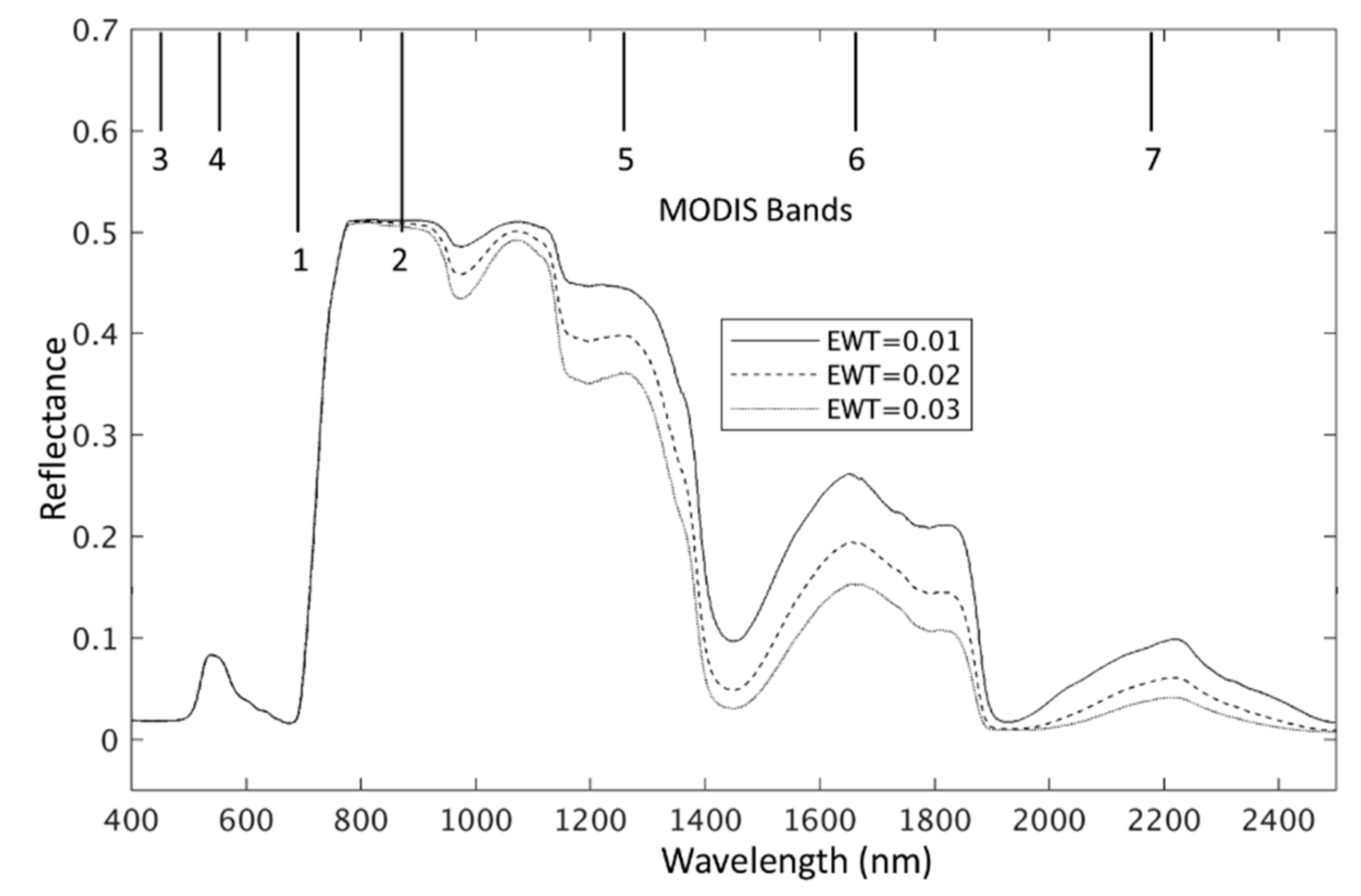The normalized difference vegetation index (NDVI) has been widely applied to monitor vegetation conditions and has been assimilated into the WCM to take the effects of the canopy on soil surface backscattering into consideration [48,49]. However, the NDVI is not the most suitable VI to be assimilated in the WCM, mainly because it is calculated based on the reflectance of the red band and the near-infrared band. The variation of the canopy’s influence on surface backscattering is mainly based on the VWC, while the red band in not that sensitive to VWC compared with shortwave infrared bands, as shown in Figure 1 [55]. Previous studies pointed out that two VIs, the normalized difference water index (NDWI), and the normalized difference infrared index (NDII) can be applied to monitor canopy VWC for various vegetation types with good results through linear or nonlinear models since they target the strong water absorption features of shortwave-infrared bands [53,54,55,56,57,58]. In this study, we applied both NDWI and NDII in the WCM to estimate SSM by considering the influence of vegetation canopy backscattering. Bao et al. 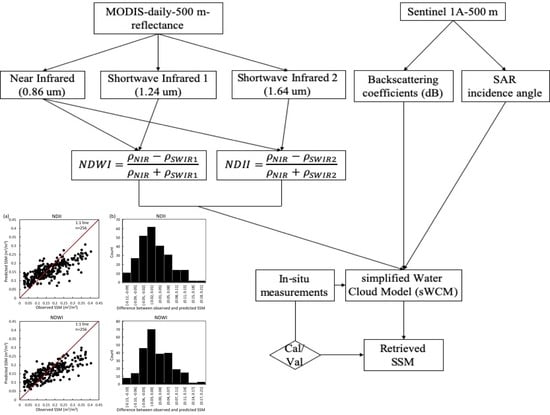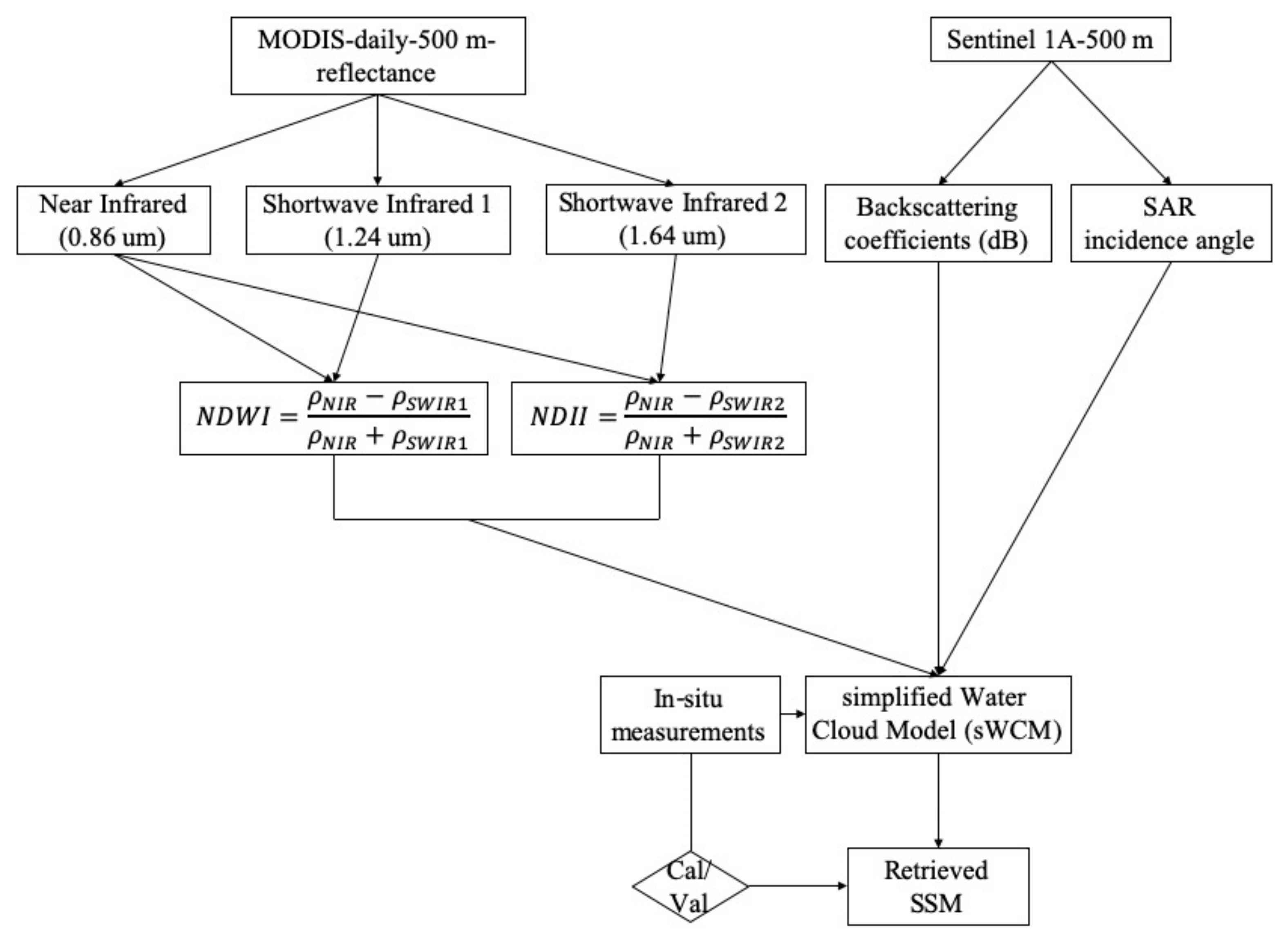tried to use Landsat retrieved VI to estimate VWC [49]. However, with Landsat 8 has the 16-day revisit cycle, and Sentinel-1A with the 12-day revisit cycle, there is always a 2–6 day time interval between Landsat 8 and Sentinel overpassing day, which makes it a big issue to fill the time gap. Landsat 8 is very sensitive to cloud cover, only limited valid satellite observations can be collected. In this study, we applied the daily MODIS reflectance products instead of combining the Sentinel-1 products on the same observing.

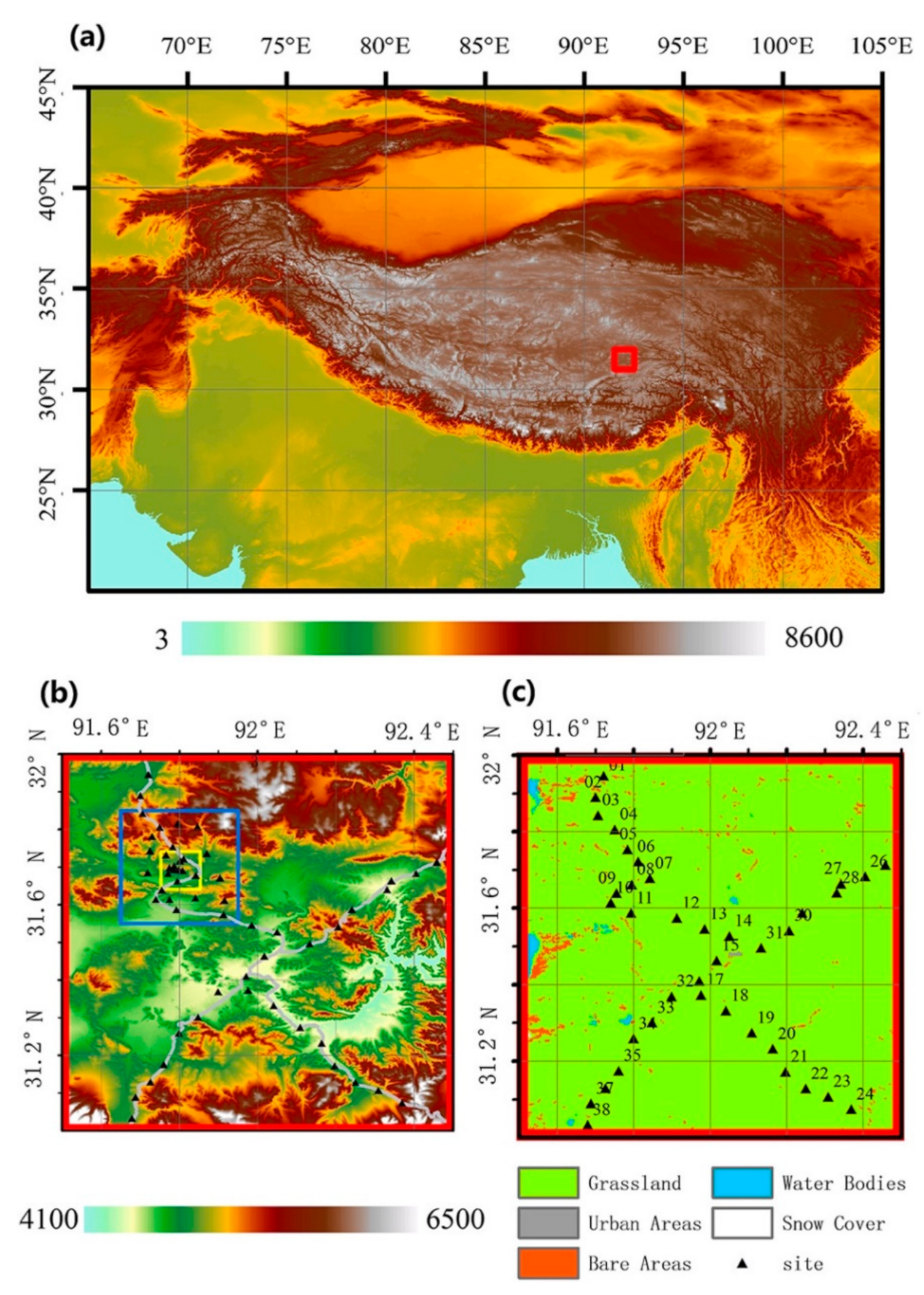
The Tibetan Plateau, the highest plateau on earth, contains a large amount of permafrost soil, widely distributed. The energy and water dynamics on this plateau is very sensitive to the climate change on the Asian continent and, subsequently, on a global scale. TP makes the monsoon on its southwestern side weaken in the summer, while the drought in central Asia consequently intensifies. The heat rising by TP in summer strengthens atmospheric circulation, and the SM condition in TP acts as an amplifier for the drought in central Asia and the monsoon in East Asia. Against the background of a changing climate, the thawing of the permafrost layer with grassland as the main vegetation type will considerably impact the water dynamics on the TP. Based on previous studies, the soil energy–water distribution and freezing–thawing processes vary spatially, and estimating SM at high spatial and temporal resolution is of great importance to develop protection measures for the plateau [59,60]. In this context, we estimated volumetric SSM (m³/m³) with vegetation cover (grassland) in the central of the TP, based on a simplified WCM (sWCM) through the soil backscattering coefficient and signal incident angle, which can be extracted from Sentinel-1 products. Since in the winter (from December to February) the soil was completely frozen, the study was conducted in spring, summer, and winter (from March to November). To eliminate the impact of backscattering coefficients from vegetation canopy, we integrate VI (NDII and NDWI) in the WCM. Both NDII and NDWI can be derived through MODIS shortwave infrared and near infrared bands. To better understand soil properties on the TP, including ST and SM at various depths, an in situ measurement network has been built in Naqu, the center of the TP, providing temporal continuous ST and SM data at four depths. We validated the retrieval method with ground measurements to demonstrate the feasibility and performance.

2. Study Area

TP is the highest plateau in the world with an average elevation of over 4000 m above sea level. Our study area is located within the center of the TP (31–32 °N,91.5–92.5 °E), covering about 10,000 km². As shown in Figure 2a,b, the study area is relatively flat, with several hills distributed. As shown in Figure 2c, over 95% of the study area is grassland, mainly alpine grasslands, but also prairie and meadows [60,61]. The growing season is short, allowing a grass height of only several centimeters [7,60], facilitating the application of remote sensing techniques in this area. The soil types are mainly silt and sand, with a clay content of less than 10%, resulting in a high drainage effect. The climate is semiarid, with an annual precipitation of about 500 mm, mostly concentrated in summer. According to long-term records, around 75% of the precipitation occurs from June to August [7,60,61]. SM shows a strong seasonal behavior, especially in terms of SSM. The annual freeze/thaw cycle considerably influences the soil water dynamics in the area, impacting SSM measurements. The annual freeze and thaw cycle of the study area starts to freeze in October, and it starts to thaw in January. From December to February, the soil surface is fully frozen. Therefore, the ground measurements were conducted from March and November.

3. Data and Methodology

3.1. Data

We applied TERRA MODIS reflectance to generate two vegetation indices (VI) since one of the shortwave infrared bands of MODIS, band 6, has broken down and cannot be applied to calculate NDII. The Sentinel-1A SAR incident angle and backscattering coefficients of the land surface were combined with each VI separately to build the sWCM. Two thirds of the in situ SSM measurements collected from the CTP-SMTMN were used to train the sWCM proposed in this study, while one third of the measurements was applied for model validation.

3.1.1. In Situ Measurements

Based on the significance of the TP for the global climate, several in situ measurement networks have been established there in the last few decades to investigate the soil–vegetation–atmosphere cycle and its relationship with the local climate [61]. In this study, we used in situ data collected from a multiscale soil moisture and temperature monitoring network in the central Tibetan Plateau (CTP-SMTMN) established by the Data Assimilation and Modeling Center for Tibetan Multi-Spheres (DAM) to evaluate SSM. There are 56 sampling sites in total at three spatial scales, measuring SM and ST at three spatial scales (1°, 0.3°, 0.1°) and four depths (0–5, 10, 20, 40 cm) from 1 August 2010 to 30 June 2016. The sensors automatically measured SM and ST every 30 minutes, calculating the average values for the past 30 minutes. The in situ measurements were validated by taking 10 undisturbed soil samples from different stations [60]. We used a large-scale network in this study, and randomly selected observations of 18 sampling sites to train the model proposed in this study; we also used observations of another eight sampling sites to validate the results retrieved by the sWCM. The geolocation of the sampling sites used for training and validation are listed in

Table 1. Geolocations of 18 sampling sites used for model training.

Site #	Longitude (°E)	Latitude (°N)	Altitude (m)	Major Soil Type
BC05	92.20	31.17	4548	Sand (49.46%)
CD02	92.41	31.68	4612	Silt (57.98%)
CD03	92.34	31.66	4518	Silt (51.59%)
CD06	92.21	31.54	4769	Silt (50.85%)
MS3475	91.72	31.95	4637	Sand (62.02%)
MS3482	91.70	31.89	4713	Silt (64.89%)
MS3488	91.71	31.84	4799	Sand (56.52%)
MS3494	91.75	31.81	4818	Silt (56.20%)
MS3501	91.78	31.75	4723	Silt (54.95%)
MS3518	91.79	31.66	4574	Sand (55.13%)
MS3527	91.74	31.61	4552	Sand (66.44%)
MS3533	91.79	31.59	4539	Silt (60.85%)
MS3545	91.91	31.57	4671	Sand (54.55%)
MS3614	91.76	31.17	4633	Sand (48.84%)
MS3620	91.73	31.13	4765	Sand (48.68%)
MS3627	91.69	31.09	4736	Sand (71.69%)
MS3633	91.68	31.03	4675	Sand (51.81%)
MSBJ	91.90	31.37	4505	Sand (58.77%)

and

Table 2. Geolocations of eight sampling sites used for model validation.

Site #	Longitude (°E)	Latitude (°N)	Altitude (m)	Major Soil Type
BC03	92.31	31.11	4690	Silt (61.05%)
BC04	92.25	31.13	4609	Sand (56.13%)
BC08	92.04	31.33	4470	Sand (63.52%)
MS3523	91.75	31.64	4570	Sand (47.43%)
MS3501	91.78	31.75	4723	Silt (54.95%)
MS3552	91.98	31.55	4574	Silt (57.71%)
MS3559	92.05	31.53	4516	Sand (55.22%)
MS3603	91.80	31.26	4630	Silt (48.54%)

, respectively.

3.1.2. MODIS

We applied TERRA MODIS in this study. The MODIS is a land surface monitoring sensor launched by the National Aeronautics and Space Administration (NASA) on board the AQAU and TERRA satellites of the Earth Observing System (EOS) mission. MODIS has 36 spectral bands in total, monitoring land surface properties, ocean properties, atmosphere properties, among others. In this study, one near-infrared band (band 2) and two shortwave-infrared bands (band 5 and band 6) were chosen. We selected the MODIS daily 500-m surface reflectance products (MOD09GA) band 2 (841–876 μm) and band 6 (1628–1652 μm) to calculate NDII, band 2, and band 5 (1230–1250 μm) to calculate NDWI. The VIs were combined with Sentinel measurements in the sWCM to estimate vegetated SSM.

3.1.3. Sentinel-1 SAR

Since only the Sentinel-1A product covered our area in 2015, it was selected for our study. Compared with the MODIS product, the main advantage of Sentinel-1 is they can be acquired under all weather conditions, and Sentinel-1 radar sensors are not affected by cloud cover. Sentinel-1 carries a C-band (5.4 GHz) SAR sensor with multi-polarization imaging capability, which supports both single polarization (HH, VV) and dual polarization (HH + HV, VV + VH). There are four imaging modes (stripmap model (SM), interferometric wide swath (IW), extra-wide swath (EW), and wave mode (WM)) for the Sentinel product, which mainly differentiate in the stripe width. The SM, IW, and EW are available in both single and dual polarization, while WV is only available in single polarization. The IW swath mode is the main acquisition mode over land and satisfied the majority of service requirements; for this reason, it was selected in our study. We applied the VV IW backscattering coefficients and incident angle measurement in the model proposed above to estimate SSM (https://www.asf.alaska.edu/sar-data-sets/sentinel-1/).

3.2. Methodology

We used one MODIS near-infrared band and two shortwave-infrared bands to calculate NDWI and NDII to represent VWC; the backscattering coefficients and incident angle were extracted from sentinel-1A SAR products. These parameters were assimilated into the simplified WCM (sWCM) to monitor SSM combining in situ measurements, as illustrated in Figure 3. Two-thirds of the ground measurements were used to train the model, while one-third were applied for model validation. For this, we randomly selected 18 sampling sites from CTP-SMTMN to train the semi-empirical sWCM and eight sampling sites for model validation.

The MODIS level-3 reflectance products were processed with the MODIS reprojection tool (MRT) conducted by NASA to subset the study area and projected to the UTM WGS84 46 zone with a 500-m spatial resolution. In addition, the Sentinel application platform (SNAP) was used to conduct the radiometric calibration/terrain calibration and to obtain the incident angle and backscattering coefficients that are required in the sWCM. The backscattering coefficients were generated through a linear conversion of the intensity of the microwave signal. Similar as in MODIS processing, SAR images were subset first to select the study area and were projected to UTM projection with a 500-m spatial resolution.

The main difference between NDII and NDWI is the wavelength of the selected shortwave-infrared band. The NDII applied near-infrared band with a wavelength of 860 μm and the shortwave-infrared band with a wavelength of 1640 μm as illustrated in Equation (1), while NDWI applied the same near-infrared band and shortwave infrared band with a wavelength of 1240 μm as illustrated in Equation (2). We calculated both NDII and NDWI through the MODIS reflectance product and applied them in the WCM separately to the estimated SSM:

$$\begin{array}{c}NDII=\frac{{\rho }_{nir}\left(860 \mu m\right)-{\rho }_{swir1}\left(1640 \mu m\right)}{{\rho }_{nir}\left(860 \mu m\right)+{\rho }_{swir1}\left(1640 \mu m\right)}\end{array}$$

(1)

$$\begin{array}{c}NDWI=\frac{{\rho }_{nir}\left(860 \mu m\right)-{\rho }_{swir2}\left(1240 \mu m\right)}{{\rho }_{nir}\left(860 \mu m\right)+{\rho }_{swir2}\left(1240 \mu m\right)}\end{array}$$

(2)

where ${\rho }_{nir}$ represents the reflectance of the near-infrared bands, ${\rho }_{swir}$, ${\rho }_{swir2}$represents the reflectance of two shortwave-infrared bands separately.

There is a linear relationship between these two vegetation indices and the VWC, which has been verified by several studies conducted in agricultural and grassland areas [54,57,58]:

$$\begin{array}{c}VWC=a\ast VI+b\end{array}$$

(3)

where a and b are empirical parameters in the linear model.

To better describe the backscattering of the soil and vegetation in vegetated areas, the original WCM adapted in this study, proposed by Attema and Ulaby, is based on the radiation transport model, considering the vegetation canopy to be uniform, with horizontal clouds, and ignoring multiple scattering. The backscattering coefficient monitored by SAR C-band signals composes surface soil scattering and scattering reflected from the vegetation; the WCM is illustrated using Equations (4)–(6):

$$\begin{array}{c}{\sigma }^0={\sigma }_{veg}^0+c\ast {\sigma }_{soil}^0\end{array}$$

(4)

$$\begin{array}{c}{\sigma }_{veg}^0=A\ast VWC\ast \cos \left(\theta \right)\ast \left(1-C\right)\end{array}$$

(5)

$$\begin{array}{c}C=\exp \left(-2\ast B\ast VWC\ast \sec \left(\theta \right)\right)\end{array}$$

(6)

where ${\sigma }^0$ is the surface backscattering, ${\sigma }_{veg}^0$ represents the vegetation canopy backscattering, ${\sigma }_{soil}^0$ represents surface soil backscattering, $\theta$ represents the SAR incident angle, and VWC can be estimated from Equation (1) to Equation (3). In this model, A and B are two empirical parameters that are applied to simulate the backscattering of vegetated surfaces as a function of the soil backscattering and the VWC. Previous studies have pointed out that the empirical parameters can be set as A equals to 0.0855 and B equals to 0.0126 at VV polarization through model assimilation [35].

Previous studies have shown that there is a good linear correlation between the soil backscattering coefficient and SSM. Therefore, the soil backscattering coefficient can be described by soil volumetric moisture SSM (Equation (7)) [48,49]:

$$\begin{array}{c}SSM=c\ast {\sigma }_{soil}^0+d\end{array}$$

(7)

where c and d are empirical parameters in the linear model.

The coefficient of determination (R²), bias, the root-mean-square error (RMSE), and unbiased RMSE were applied to evaluate the retrieved SSM results based on in situ measurements. These evaluators mentioned above were calculated via Equations (8)–(11):

$$\begin{array}{c}{R}^2=\frac{{{\displaystyle \sum }}_{i=1}^n{\left(P_i-\overline{O}\right)}^2}{{{\displaystyle \sum }}_{i=1}^n{\left(O_i-\overline{O}\right)}^2}\end{array}$$

(8)

$$\begin{array}{c}bias=\frac{{{\displaystyle \sum }}_{i=1}^n\left(O_i-P_i\right)}{n}\end{array}$$

(9)

$$\begin{array}{c}RMSE=\sqrt{\frac{1}{n}{\displaystyle \sum }_{i=1}^n{\left(O_i-P_i\right)}^2}\end{array}$$

(10)

$$\begin{array}{c}ubRMSE=\sqrt{{\left(RMSE\right)}^2-{\left(bias\right)}^2}\end{array}.$$

(11)

where n is the number of observations for validation, P is the predicted results, O is the in situ observation, and $\overline{O}$ average of all observed value.

4. Results and Discussion

We estimated vegetated SSM within the central TP through sWCM combining multi-source satellite observations (MOD09 and Sentinel-1A SAR) and in situ measurements from CTP-SMTMN. In situ measurements were also applied to validate the monitoring results. Based on the statistical results obtained for 2015 (

Table 3. Statistical results of the methods proposed in this study (all sites), with R² (coefficient determination), RMSE (root-mean-square error) (m³/m³), ubRMSE (unbiased root-mean-square error) (m³/m³), and bias (m³/m³).

Vegetation Index Applied	R2	RMSE (m3/m3)	ubRMSE (m3/m3)	bias (m3/m3)
NDII	0.4513	0.0609	0.0603	0.0085
NDWI	0.4264	0.0613	0.0607	0.0083

), the sWCM integrating MODIS and SAR observations can be applied to effectively retrieve SSM in the study area. Both NDII and NDWI were suitable (R > 0.6) and can be integrated into the sWCM for SSM monitoring. The NDII worked relatively better, with a higher R², a lower RMSE, and a lower ubRMSE. Both NDII-sWCM and NDWI-sWCM slightly overestimated SSM with positive bias values over the study.

Table 4. Statistical results of NDII-sWCM (normalized difference infrared index- simplified water-cloud model) for each validation sites, with R² (coefficient determination), RMSE (root-mean-square error) (m³/m³), ubRMSE (unbiased root-mean-square error) (m³/m³), and bias (m³/m³).

Site #	RMSE (m3/m3)	ubRMSE (m3/m3)	bias (m3/m3)
BC03	0.0591	0.0589	−0.0051
BC04	0.087	0.0610	0.0620
BC08	0.0656	0.0654	0.0043
MS3501	0.0926	0.0470	0.0798
MS3523	0.0368	0.0368	−0.0005
MS3552	0.0347	0.0346	−0.0020
MS3559	0.0407	0.0392	−0.0112
MS3603	0.0389	0.0363	−0.0141

and

Table 5. Statistical results of NDWI-sWCM (normalized difference water index- simplified water-cloud model) for each validation sites, with R² (coefficient determination), RMSE (root-mean-square error) (m³/m³), ubRMSE (unbiased root-mean-square-error) (m³/m³), and bias (m³/m³).

Site #	RMSE (m3/m3)	ubRMSE (m3/m3)	bias (m3/m3)
BC03	0.0564	0.0553	0.0112
BC04	0.0941	0.0681	0.0650
BC08	0.0724	0.0507	−0.0521
MS3501	0.0839	0.0441	0.0714
MS3523	0.0308	0.0296	−0.0087
MS3552	0.0389	0.0389	0.0009
MS3559	0.0415	0.0407	−0.008
MS3603	0.0395	0.0371	0.0143

are the statistical results of NDII-sWCM and NDWI-sWCM, respectively.

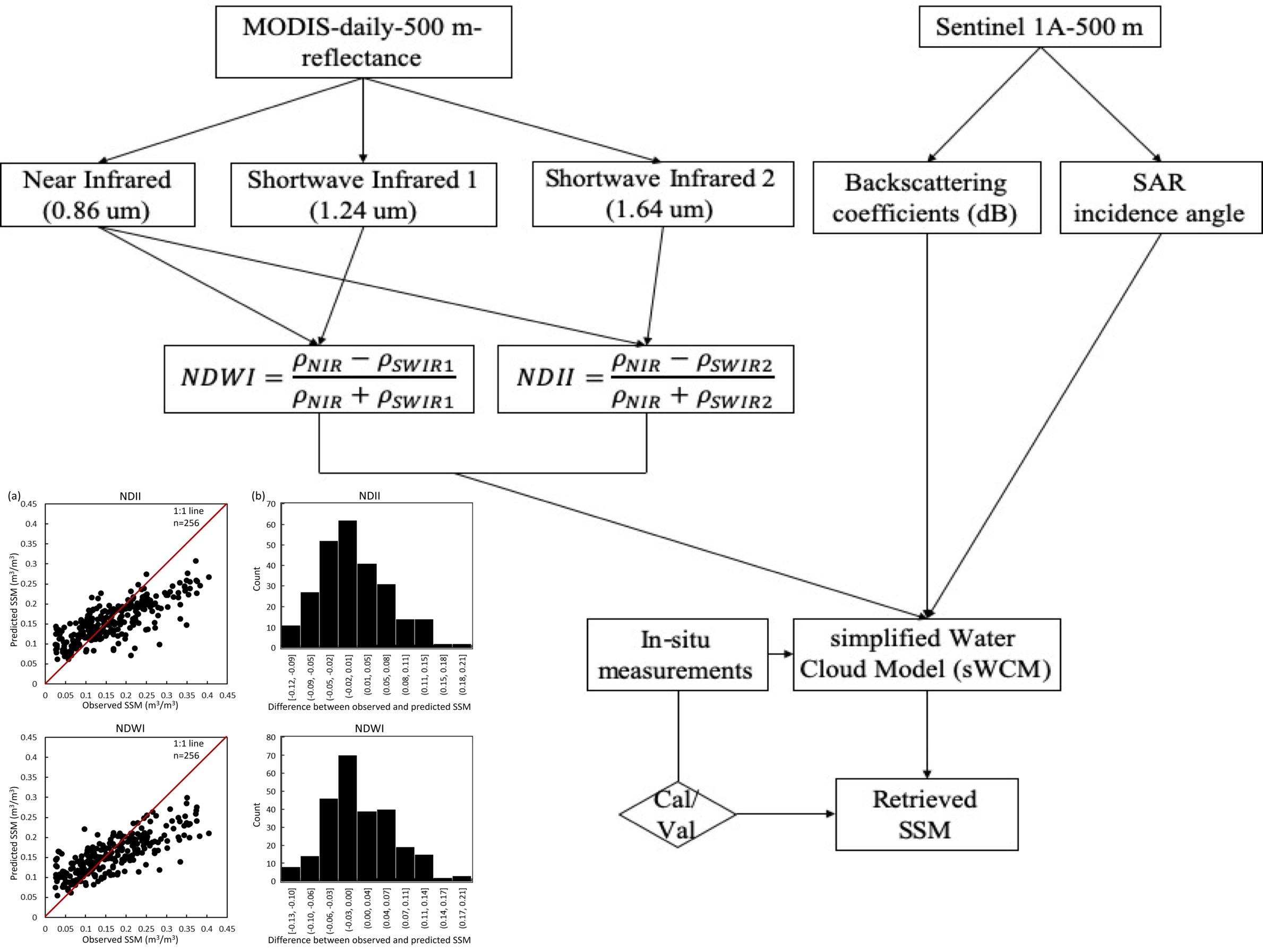
Figure 4a illustrates the scatterplots between observed and predicted SSM values, considering VI as NDII or NDWI separately (with 1:1 red line shown). Both NDII and NDWI overestimated SSM under low SSM conditions (in situ SSM < 0.15 m³/m³), and both VIs underestimated SSM under high SSM conditions (in situ SSM > 0.2 m³/m³). Figure 4b represents the histogram of the differences between observed and predicted SSM values, the value accumulated (over 70%) between −0.05 to 0.05 m³/m³ for NDII, between −0.06 to 0.07 m³/m³ for NDWI.

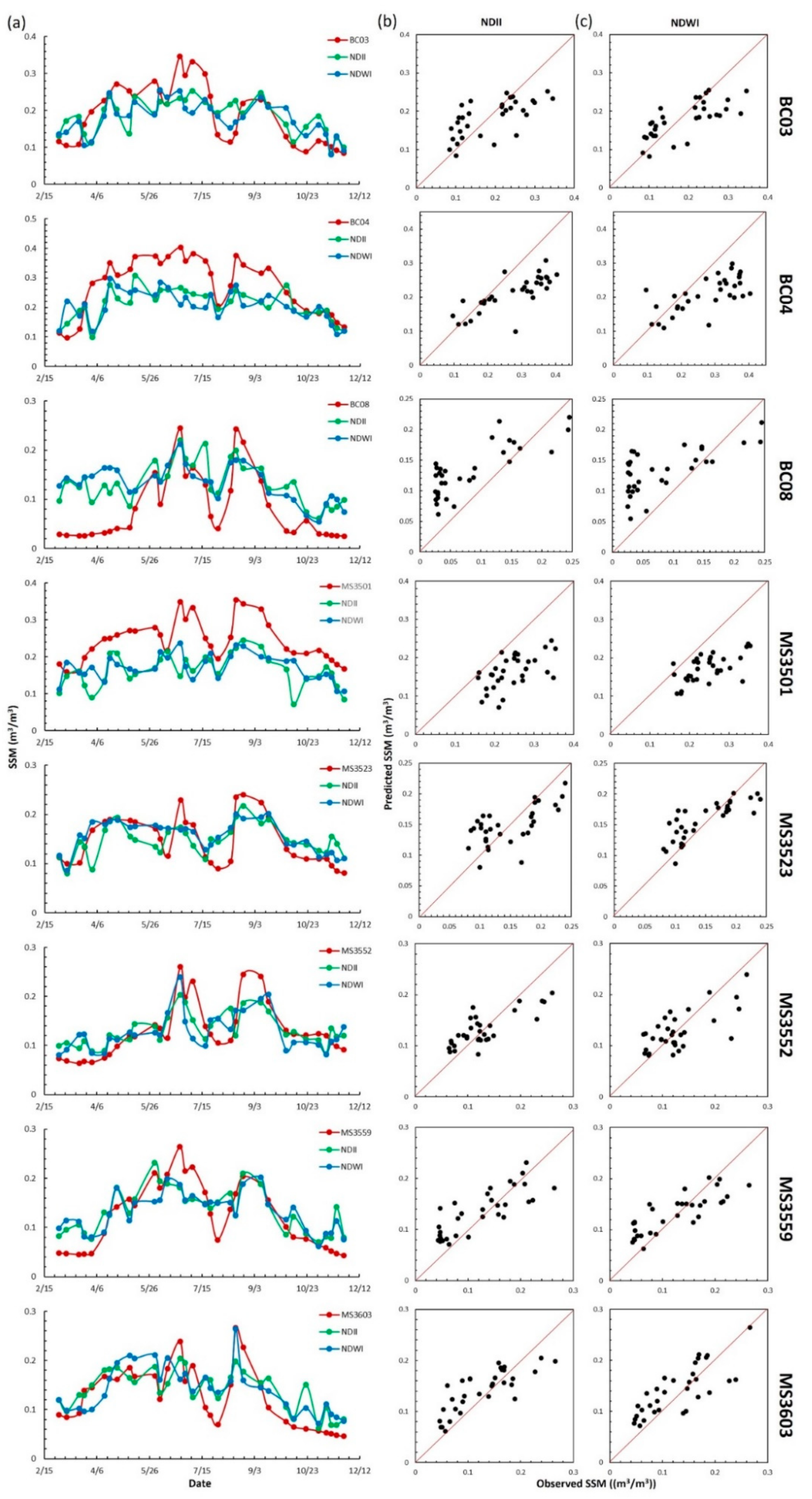
Figure 5a shows the time series of observed and predicted SSM values for eight validation sites separately. The red line represents the observed SSM values, green line represents the predicted SSM values with NDII integrated in sWCM, blue line represents the predicted SSM values with NDWI integrated in sWCM. For sites MS3552 and MS3603, the trend of predicted SSM (NDII-sWCM and NDWI-sWCM) matched the observed SSM quite well. For all sites, summer (May to August) has the highest SSM values which is consistent with the information provided above, that summer has the most precipitation within the year. Observed SSM values drop rapidly at the beginning of August for all sites, predicted SSM values of some sites drop rapidly at the same time. Such situation is not understood yet. Figure 5b,c illustrates the scatter plot between observed and predicted SSM values when NDII or NDWI were applied in the sWCM separately. In one site (BC08), sWCM overestimated SSM for the whole study period; while in two sites (BC04 and MS3501), sWCM underestimated SSM for most of the study period. In three sites (BC03, MS3523, and MS3552), SSM was overestimated when it was low and underestimated when it was high, which is consistent with the results from Figure 4. In two sites (MS3559 and MS3603), the scatterplots were distributed along the 1:1 red line. When the same parameters were applied, different validation sites yielded different results.

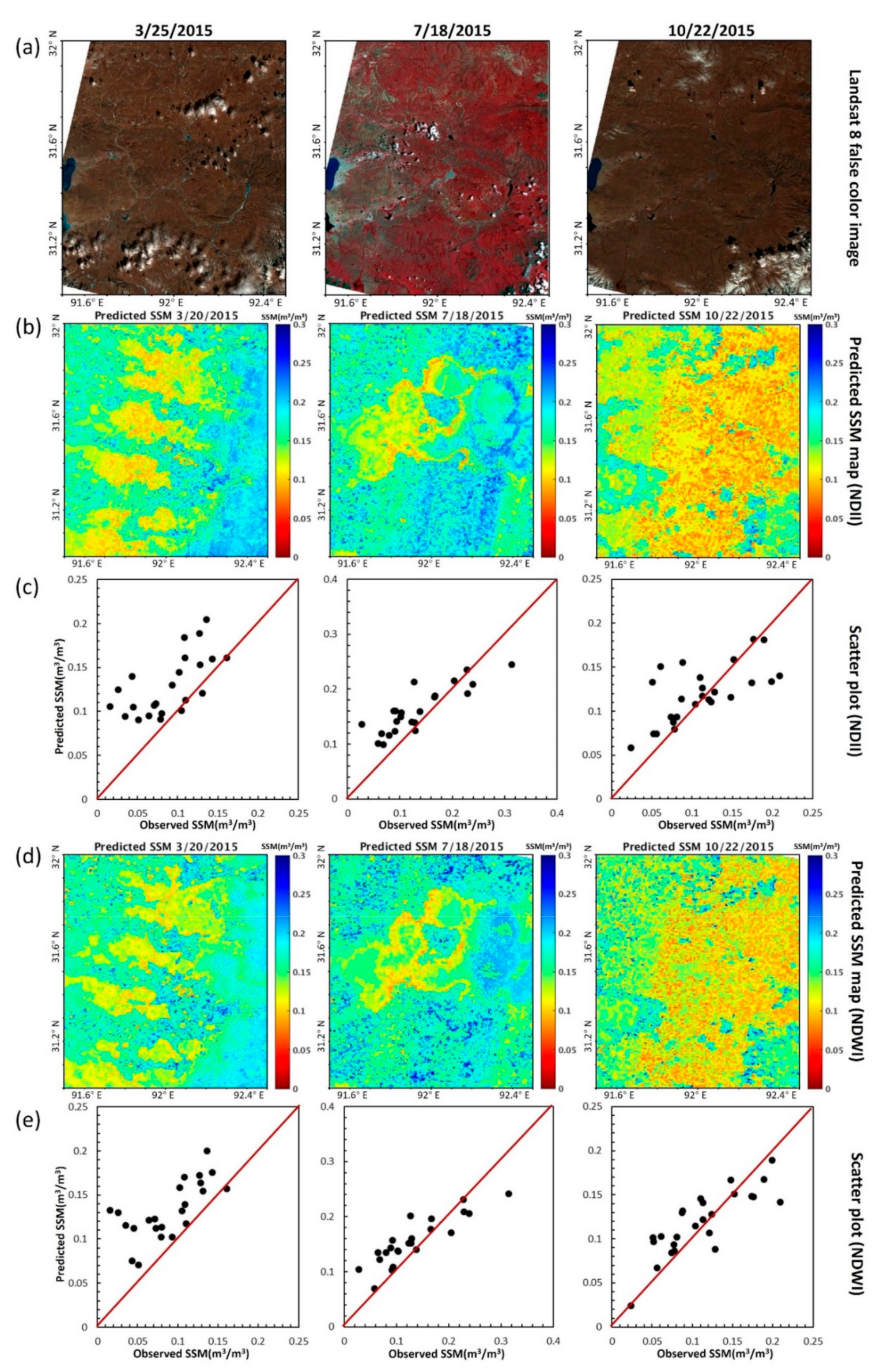
Figure 6a shows the Landsat 8 false color image using the reflectance band (band1) as red, the shortwave-infrared band (band2) as green, and the near-infrared band (band3) as blue, where red indicates regions with vegetation cover and brown indicates bare soil. From left to right, the images acquired are on 25 May, 18 July, and 22 October. Based on the false color images, in May and October, the study area contained mostly bare soil, while in July, it was fully covered by grass. Figure 6b,d, from left to right, are the generated SSM images when NDII or NDWI were integrated in the sWCM separately. Figure 6c,e show the scatter plots between observed and predicted SSM values when NDII or NDWI were applied in the sWCM, respectively. In spring, both NDII and NDWI overestimated SSM. In summer and autumn, the distribution was along the 1:1 red line and the scatterplots were also accumulated along the 1:1 red line, suggesting that the model works better for soil with vegetation cover compared with bare soil. We observed a spatial-temporal pattern of SSM distribution, with the highest and lowest levels in summer and winter, respectively. Most likely, this is because the active layer starts to thaw in spring, resulting in a rapid increase in SSM. In contrast, in autumn and winter, the soil is mostly frozen, with decreased SSM levels. In spring, the eastern part of the study area showed relatively high SSM values when compared to the western part, while in summer, SSM was lowest in the central part. In winter, the lowest levels were observed for the central and eastern parts. Both images generated by NDII-sWCM and NDWI-sWCM illustrate the same distribution. The NDII-sWCM show lower SSM values compared to the NDWI-sWCM for spring, summer, and autumn.

Although the model proposed in this study achieved good results in the grassland area in TP, we recognize that there are some uncertainties. First, there were uncertainties from satellite measurements, as the MODIS solar bands have associated atmospheric uncertainties. Second, some uncertainties were associated with the ground observations, mainly caused by technique design and experimental design, although calibration and validation were conducted. Third, we estimated the backscattering of the vegetation canopy mainly based on the VWC, but there are other factors that also affect the surface backscattering of active microwave signals such as soil surface roughness. Fourth, the WCM only considers the surface backscattering composed of backscattering from soil and vegetation and assumes there is no reflection within the vegetation canopy. Such assumption can, however, not be made for the “real world”. Soil texture and soil roughness are important factors that affect the backscattering of C-band signals, and omitting such factors may cause uncertainties in the retrieved SSM values when there is a vegetation cover. In addition, both NDII-sWCM and NDWI-sWCM were more suitable when there was a vegetation cover, and the model may need to be revised in this regard. From the scatter plots shown in Figure 4a, we recognized that sWCM underestimates SSM under high SSM conditions in summer and overestimates SSM under low SSM conditions in spring and autumn. The uncertainties within field experiments may induce the monitoring errors. From time series shown in Figure 5a, we see that although the average in situ SSM value is relatively high in summer, for each sampling site the SSM observations vary a lot. There are days for some sites with extremely low SSM values, while other sites with relatively high SSM observations. Besides that, both MODIS and Sentinel-1A only measure the land surface properties, there may be a delay for surface condition change caused by SSM, and it may not be timely observed by satellite sensors. Although the soil temperature is above 0 °C in March and November within the study area, there may exist ice crystals in the soil, the heat absorption or release within the phase change of water may also affect SSM monitoring. In this study, we analyzed the study period together, while the empirical parameters in the sWCM varies under different conditions. If different seasons were studied separately, the monitoring results may be improved.

5. Conclusions

We mapped SSM at a 500-m resolution for a vegetated area (grassland) of the TP during the non-frozen period (March to November in 2015), combining TERRA MODIS and Sentinel-1 SAR products using the sWCM proposed in this study. The method is based on the relationship between SSM and SAR C-band backscattering, which is based on the soil dielectric variation due to changes in the water content. The impact of vegetation canopy backscattering on the signal SAR received can be dealt with by integrating two VIs (NDII and NDWI) into the WCM, resulting in the models NDII-sWCM and NDWI-sWCM. Both models are well suited for vegetation SSM monitoring, with NDII-sWCM showing better results.

The main contributions of this study are: 1) monitoring of the SSM in a high-latitude permafrost region by combining optical and microwave products during the non-frozen period; 2) elimination of the effects of vegetation canopy backscattering on SAR by assimilating two VIs in the original WCM, resulting in the two simplified water-cloud models NDII-sWCM and NDWI-sWCM. The retrieved SSM values were validated by in situ measurements from CTP-SMTMN. Both NDII and NDWI can be applied in the sWCM to retrieve SSM values for vegetated areas; 3) determination of the temporal and spatial patterns of SSM within the study area from March to November 2015. The central TP showed the highest values in summer and the lowest ones in winter, indicating that the spatial distribution of SSM varies throughout the year. The retrieved 500-m SSM values for vegetated areas are of great importance for further ecosystem and climate research over TP, since the soil water content plays a key role in the water cycle and energy transfer between land and atmosphere via evapotranspiration.