Combination of Linear Regression Lines to Understand the Response of Sentinel-1 Dual Polarization SAR Data with Crop Phenology—Case Study in Miyazaki, Japan

Abstract

This study investigated the relationship between backscattering coefficients of a synthetic aperture radar (SAR) and the four biophysical parameters of rice crops—plant height, green vegetation cover, leaf area index, and total dry biomass. A paddy rice field in Miyazaki, Japan was studied from April to July of 2018, which is the rice cultivation season. The SAR backscattering coefficients were provided by Sentinel-1 satellite. Backscattering coefficients of two polarization settings—VH (vertical transmitting, horizontal receiving) and VV (vertical transmitting, vertical receiving)—were investigated. Plant height, green vegetation cover, leaf area index, and total dry biomass were measured at ground level, on the same dates as satellite image acquisition. Polynomial regression lines indicated relationships between backscattering coefficients and plant biophysical parameters of the rice crop. The biophysical parameters had stronger relationship to VH than to VV polarization. A disadvantage of adopting polynomial regression equations is that the equation can have two biophysical parameter solutions for a particular backscattering coefficient value, which prevents simple conversion from backscattering coefficients to plant biophysical parameters. To overcome this disadvantage, the relationships between backscattering coefficients and the plant biophysical parameters were expressed using a combination of two linear regression lines, one line for the first sub-period and the other for the second sub-period during the entire cultivation period. Following this approach, all four plant biophysical parameters were accurately estimated from the SAR backscattering coefficient, especially with VH polarization, from the date of transplanting to about two months, until the mid-reproductive stage. However, backscattering coefficients saturate after two months from the transplanting, and became insensitive to the further developments in plant biophysical parameters. This research indicates that SAR can effectively and accurately monitor rice crop biophysical parameters, but only up to the mid reproductive stage.

1. Introduction

Rice is a staple food, feeding approximately half of the world’s population. Estimates indicate that, by the mid-twenty first century, one of the biggest challenges will be to feed the nine billion people of the world [1]. Therefore, to address this challenge, cereal grain production, especially systematic rice monitoring, plays an important role in sustainable development and ecological planning. Several different types of remote sensing technologies could be used to measure rice growth parameters including: leaf area index (LAI), plant height, biomass, and canopy [2,3]. Better monitoring of these parameters could help us better manage the crop development conditions and ultimately increase rice production. Remote sensing monitoring from different platforms, ranging from the field level to satellite, can provide information that is useful to identify the status and condition of various plant and soil parameters throughout the growing season [4]. Examples of this include the following: early season information about soil fertility and moisture conditions, mid-season crop monitoring for pest and disease management, and growth trajectory analyses and yield estimation throughout the growing season. Remote sensing data also provide a convenient method for relating point observations to spatial management plans [4]. Satellite remote sensing has proven to play a key role in supporting food security initiatives, and the community has achieved significant progress so far based on this technology. Optical remote sensing has been utilized for agricultural decision support systems via crops monitoring, such as by using the vegetation related products of Moderate Resolution Imaging Spectroradiometer (MODIS), combined with agro-metrology metrics such as precipitation, temperature, solar radiation, and soil moisture [5]. Examples of these tools are found in several literatures [6,7,8,9,10,11].

Landsat and its relevant derivative indices have spectral bands sensitive to rice paddy conditions [12,13]; however, phenological differences between scenes and low temporal frequency in historical archives have limited mapping of rice at moderate scales over large areas [5]. More than 70% of rice production is during the monsoon or rainy season [14], when cloud cover is extensive [15]. Cloudy regions such as South Asia, often have periods of no or few clear-sky Landsat scenes [5]. A lack of high temporal frequency of optical imagery is a limitation on rice cultivation mapping over large regions. In the case of our study area, only one clear-sky Landsat image was available during the entire cultivation season of paddy rice in 2018 (April to July), and the image was just before harvest. Clear-sky high-resolution optical images are rarely available from the beginning to the mid cultivation season, because the cultivation is conducted during rainy season. This is an example of the limitation in phenological monitoring of rice crop using optical sensors.

Compared with optical sensors, synthetic aperture radar (SAR) can monitor surfaces in any weather conditions, which is particularly useful for mapping and monitoring rice in South and Southeast Asia, where frequent cloud cover and precipitation are expected during the cultivation seasons [5,12]. The SAR system transmits electromagnetic pulses and receives the echoes of the backscattered signal from the Earth’s surface. Microwave is used for SAR monitoring. Typical wavelengths adopted by satellite-SAR monitoring are 2.5–4 cm (X-band; such as adopted by TerraSAR-X satellite), 4–8 cm (C-band; such as adopted by Sentinel-1 satellite), and 15–30 cm (L-band; such as adopted by ALOS-2 satellite). The amplitude and phase of the backscattered signal changes by the physical characteristics of the surface (such as surface geometry and roughness), and the electrical permittivity [16]. For rice applications, SAR observations at the relevant configuration are sensitive to growth stages, biomass development, plant height, leaf-ground double bounce, soil moisture, and inundation frequency and duration [15,17]. During the rice transplantation period, the surface contribution of a rice paddy causes low backscatter. In the plant tillering period, the volumes of haulm and the leaves increase, and the backscatter response increases with more interaction and volume scattering. Consequently, as crops peak and approach harvest, it causes a decrease in backscatter. This makes SAR particularly useful for mapping rice extent, inundation, and cropping intensity, considering dynamic range and scattering mechanisms of the rice life cycle. The interaction mechanism between the radar waves and vegetation canopy has three components: (1) volume scattering, (2) scattering from the ground made by vegetation layer, and (3) multiple scattering between the volume and ground [18]. X- and C-bands are suitable to retrieve canopy biophysical parameters because images produced from short wavelength SAR, such as X- and C-bands, mainly interacts with the top portion of the canopy layer [19]. The relationship between rice growth parameters and radar backscattering coefficients was studied by Kurosu et al. [20]. They used the C-band VV (i.e., vertical transmitting, vertical receiving) polarization data from the European Remote Sensing (ERS-1) satellite. However, few studies investigated using C-band SAR data. These studies have mainly focused on the relationship between the backscatter coefficients from rice fields and rice growth parameters. Moreover, HH (i.e., horizontal transmitting, horizontal receiving) or VV and the ratio of HH/VV backscattered coefficients are frequently used data sets in the past studies that indicate high correlations with rice growth stages [18,21]. In all these studies, the cross polarized HV (i.e., horizontal transmitting, vertical receiving) or VH (the reverse of HV) backscatter was rarely focused on, possibly because of the limited availability of SAR data in terms of time series and polarization. Sentinel-1 radar platform lunched by the European Space Agency is able to provide timely and precise high-resolution data [22]. Le Toan et al. reported that, for X-band SAR data of HH and VV polarization, both HH and VV increased because of the increment in the vegetation cover vertical structures, but VV is more sensitive to changes in vegetation cover during the vegetative stages [23]. This idea is further supported by Mansaray et al.—even though VV polarization produces higher backscatter coefficients values, VH polarization constantly increases and is more sustained compared with VV, where saturation is reached during the tillering stage [24].

In this study, we introduce the monitoring of rice growth parameters using multi-temporal Sentinel-1 VH and VV polarization SAR images. Plant height, green vegetation cover, LAI, and the total dry biomass were acquired by fieldwork, and the coefficient of determination (R²) between the parameters and the backscattering coefficient derived from SAR data were investigated. While previous studies typically analyzed the relationship between plant biophysical parameters and the SAR backscattering coefficients using a single linear or polynomial regression line, this study attempts to express the relationship using the combination of two linear-regression lines, which is unique to this study. The two-linear-line approach taken in this study helps to clarify the turning-point of the response of SAR backscattering signals to rice plant phenology. Also, the approach has the potential to easily estimate the plant biophysical parameters by SAR backscattering coefficients.

2. Materials and Methods

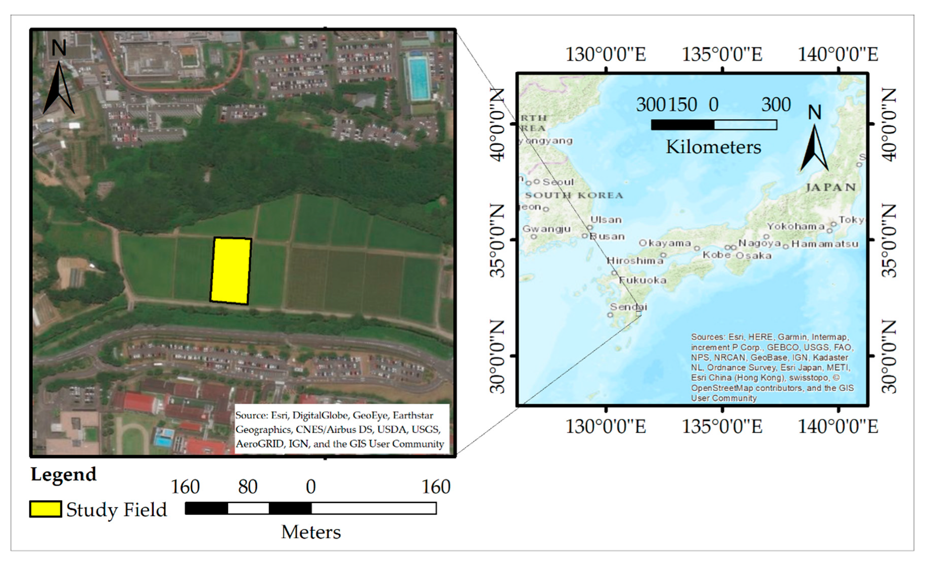
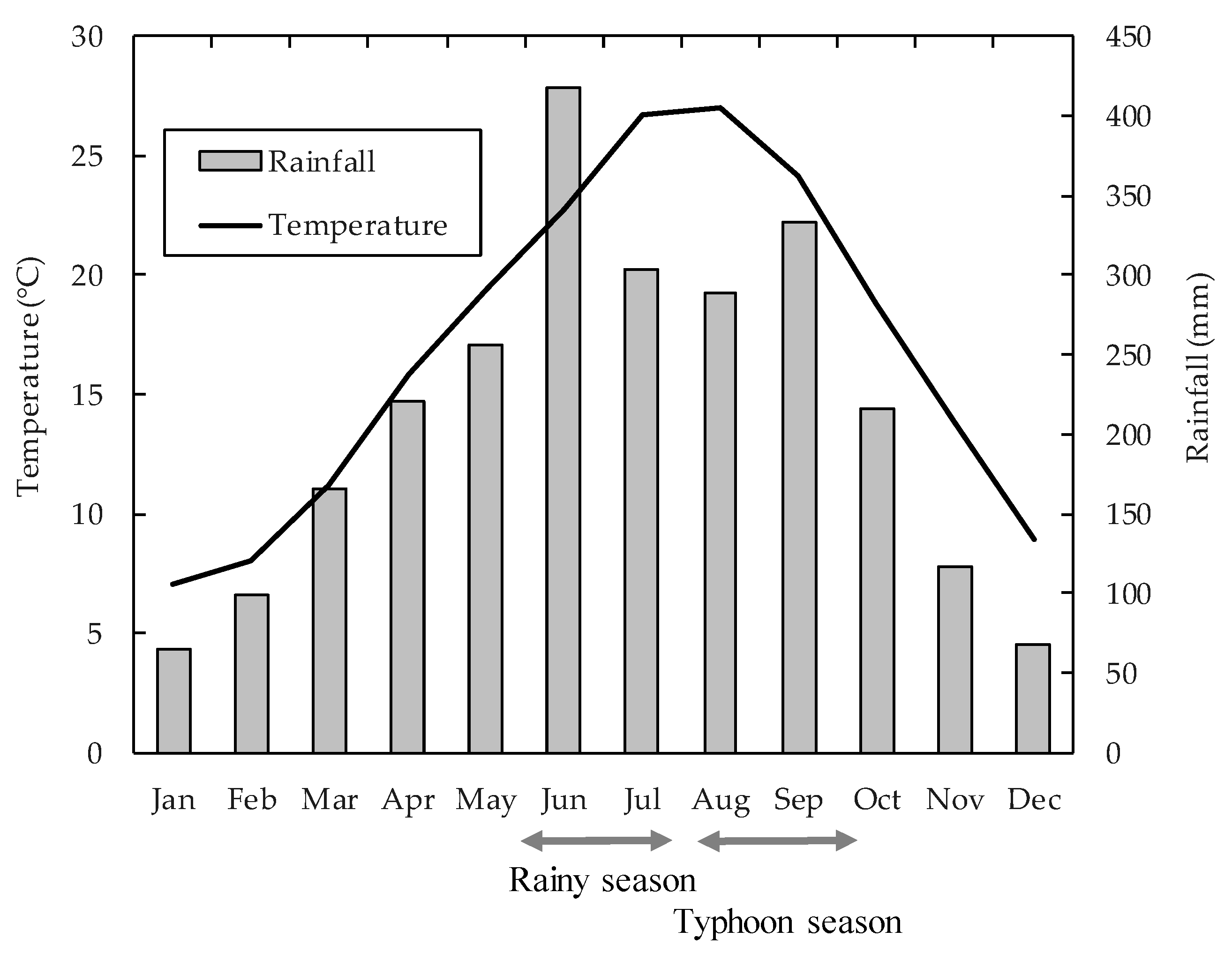
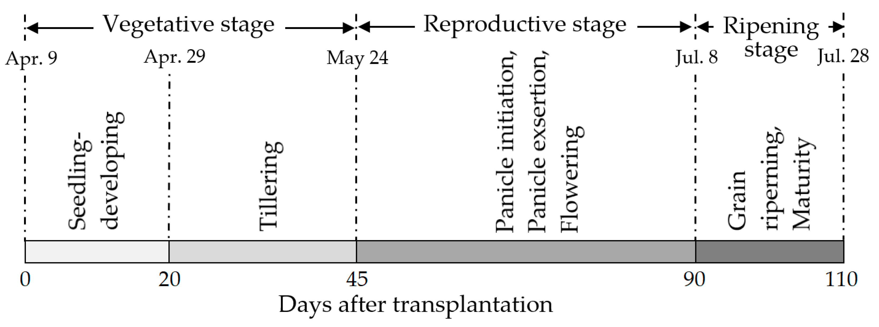
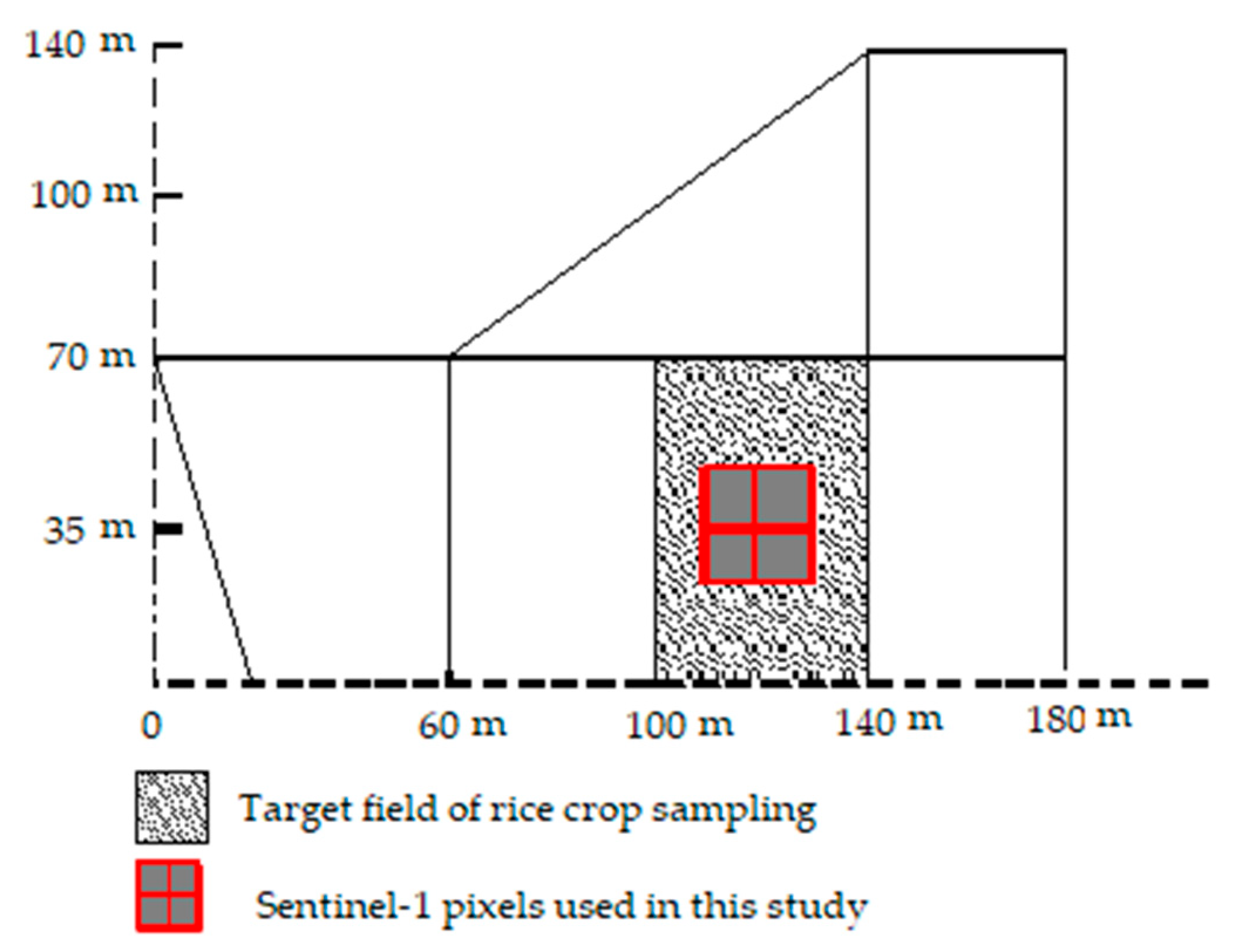
2.1. Study Area

The study field is in the Kibana Agricultural Science Station of the University of Miyazaki, in the Miyazaki prefecture of Japan (Figure 1). The study area lies at a base elevation of approximately 21 m above sea level and it is located at 31°50′14″ north and 131°23′56″ east. The climate of Miyazaki is humid subtropical, with hot and humid summers and cool winters. The average annual temperature is 17.1 °C, and annual precipitation is 2550 mm. Figure 2 shows the monthly average air temperature and rainfall in Miyazaki. The primary rainy season is from early June to mid-July. The season is called as “plum rain” and a large amount of the precipitation is a result of the East Asian monsoon system. In 2018, more than half of the days in June had recorded precipitation around the study area. The monsoon rain is a fundamental water resource for paddy rice cultivation in this area. Another peak of monthly precipitation appears in August to September, which is typically from short-term heavy rains brought by typhoons. Rice is the major staple food in Japan. Popular Japanese rice varieties, Oryza sativa ‘Koshihikari’ and ‘Hinohikari’, are most commonly cultivated around the study area. The first variety, which was planted in the study field, is typically planted in early season (transplants in late March to early April and harvest in late July) for the purpose of avoiding the risk of damage by typhoons in late summer; the later variety is planted in normal season (transplants in June and harvest in October). Figure 3 represents the rice development stages in the study area during 2018, determined by actual field surveys, following the framework of rice development stages used by Wu et al. [25]. The vegetative stage lasts for about 45 days, while the reproductive and flowering stages last for 45 and 20 days, respectively. The number of days slightly changes by year and farmer, depending on the weather conditions and cultivation practices.

2.2. Data Acquisition and Analysis

This study compares Sentinel-1 VH and VV backscattering coefficients with ground-measured biophysical parameters of a rice crop, to investigate the potential and limitations in estimating the biophysical parameters used by satellite SAR monitoring.

Table 1. Data used in this study. VH, vertical transmitting, horizontal receiving; VV, vertical transmitting, vertical receiving; LAI, leaf area index.

Data Type	Items	Data Acquisition Dates in 2018
Satellite images	Sentinel-1A, VH and VV polarization images	10 April, 22 April, 4 May, 16 May, 28 May, 9 June, 21 June, 4 July, 15 July, and 27 July
Ground-measured biophysical parameters of rice crop	Plant height Green vegetation cover LAI Total dry biomass	Same as above

summarizes the data used in this study.

2.2.1. Satellite Images

Ten Sentinel-1A time series images of the study area were acquired for the entire cultivation season from April to July 2018. The dates of the image acquisitions are given in Table 1. Sentinel-1 ground range detected (GRD) data of dual polarization (VH and VV polarization), acquired with interferometric wide (IW) mode, were used in this study. The GRD image products with the IW mode are provided by 10 m × 10 m pixel size, but the reference spatial resolution is 20 m × 22 m (range and azimuth directions, respectively), because the product is created by the multi-look procedure of IW images [26]. The acquired SAR images were preprocessed using ESA’s open source Sentinel-1 Toolbox [21]. The process includes radiometric calibration, terrain flattening, and geometric correction. Topographic variations can dominate the radiometric backscatter signal strongly because of the local area illuminated within each azimuth and slant range [27]. The reference area used within the beta naught (β⁰), sigma naught (σ⁰), and gamma naught (γ⁰) backscatter conventions is described by Small [28]. Each convention differs in their choice of definition. The β⁰ convention is the slant range plane itself [27]. The contents of images conforming to its convention are not subjected to modifications based on ellipsoid or terrain Earth models [28]. σ⁰ is the ground as modeled by an ellipsoidal Earth. For γ⁰, the area is the projection in the plane perpendicular to the slant range direction [29]. In our study, first, the radiometry of the SAR backscatter product was transformed into β⁰ backscatter convention, as is also recommended by Small et al. [30]. Secondly, the range Doppler terrain correction was applied. In this process, once the DEM integration was completed, the normalization was performed by converting β⁰ to γ⁰. In this study, the averages of VH and VV polarization backscatter signals read by four pixels from the center of the crop sampling field were used. The locations of the sampling pixels are shown in Figure 4. The study area was composed of five paddy rice fields that were all managed similarly. Considering the 20 × 22 m effective resolution of Sentinel-1A GRD images, the sampled SAR backscatter signals used in this study are not affected by surface conditions outside of the study area.

2.2.2. Ground Measurements of Plant Biophysical Parameters

Field surveys were conducted simultaneously with the dates of satellite image acquisitions, to obtain ground-measured plant height, green vegetation cover, LAI, and total dry biomass of rice crop. The actual field conditions during the cultivation period are shown in Figure 5. Representative plant height for an image date was determined by averaging the measurements at ten different locations in the study field. The standard deviations for the 10 samples, indicating the spatial variation of the plant height, were small (1 to 4 cm) in the vegetative and reproductive stages, and large (7 to 10 cm) in ripening stage. The spatial heterogeneity of plant height in the ripening stage was the result of different degrees of rice ears hanging. For green vegetation cover, ten photo image samples were taken from 70 cm above the top of the plant canopy, and the average fractional green canopy cover of rice plant was analyzed by a smartphone application, Canopeo [31]. The fractional green canopy cover is a key variable for determining canopy development, light interception, and evapotranspiration. The average standard deviation of 10 samples was 6%. In each observation, four plant hills that represent the average conditions of the field were sampled for measurements of LAI and dry biomass. ImageJ software [32] was used to compute LAI values by sampled leaves after scanning.

2.2.3. Data Analysis

The ground-based biophysical parameters were compared with VH and VV polarization backscattering coefficients of Sentinel-1A, to analyze the relationship between plant biophysical parameters and the SAR backscattering coefficients. The relationships were analyzed using two types of regressions. The first approach describes the relationship with a single polynomial regression equation determined by the least-square method, which is a traditional method of statistical analysis popularly used in this type of study. Another method attempts to describe the relationship by the combination of two linear regression lines. The concept of the two-linear-lines method is illustrated in Figure 6. The basic assumption of this approach is that the SAR backscattering coefficients first linearly increases as the rice plant develops (first period in Figure 6), and then the backscattering coefficient reaches a saturation level at a specific date termed the “turning point” during the cultivation season. In this research, the turning point is defined as the point where the R² of the linear regression for the first period reaches its maximum. The R² of the linear regression for the second period (Figure 6) is expected to be a small value, because the SAR backscattering coefficient is saturated in the second period, and thus the backscattering coefficients no longer explain the further changes in plant biophysical parameters.

3. Results and Discussion

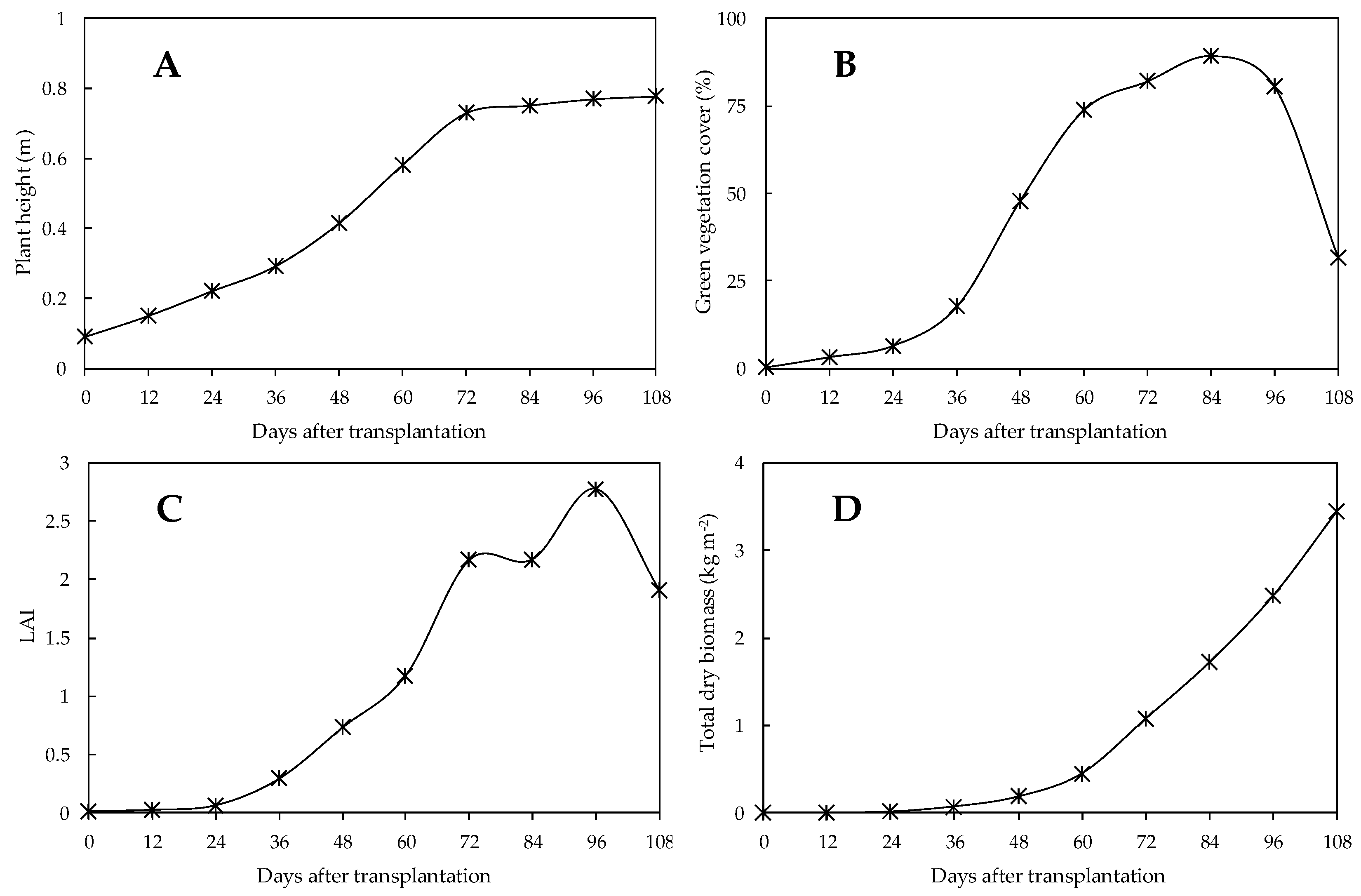
3.1. Temporal Changes in Plant Biophysical Parameters

Figure 7 shows ground-measured biophysical parameters of the rice crop (plant height, green vegetation cover, LAI, and total dry biomass) in the study field. Plant height (Figure 7A) constantly increased until around 72 days after transplant (middle of reproductive stage). The green vegetation cover (Figure 7B) gradually increased in the early vegetative stage, and then rapidly increased during the late vegetative stages. The green vegetation cover maintained at maximum during the reproductive stage, and then rapidly dropped during the ripening stage when the leaves turned yellow. LAI (Figure 7C) had a similar trend as the green vegetation cover, with some delays in the timing. The total dry biomass (Figure 7D) did not significantly increase during the vegetative stage, and constantly increased during the reproductive and ripening stages.

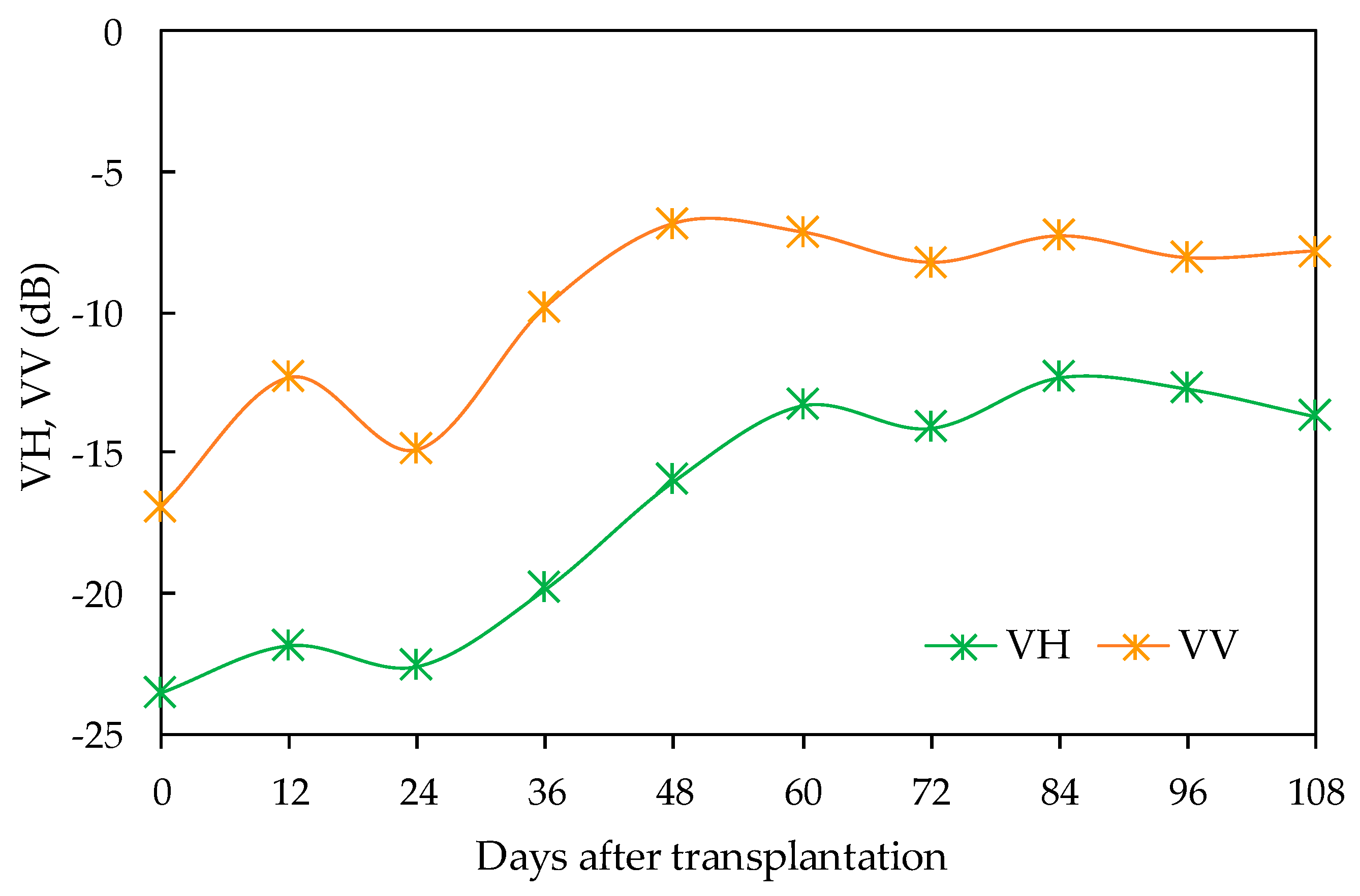
3.2. Transitions in VH- and VV-bands Backscattering Coefficients

Figure 8 shows the temporal variation in VH- and VV-bands’ backscattering coefficients. The numbers are the averages of four pixels from the center of the study field (Figure 4). Throughout the cultivation season, VV is higher than VH. Both VH and VV backscattering coefficients were the lowest during the initial period of rice cultivation. During this period, green vegetation cover was low (Figure 7B), and the dominant surface observed by satellite is the water surface flooded in the paddy field. The backscattering coefficients increased during the late vegetative stage, and became stable after 48 days (VV) or 60 days (VH). This trend in the backscattering coefficients agrees with those in previous studies [2,25,33].

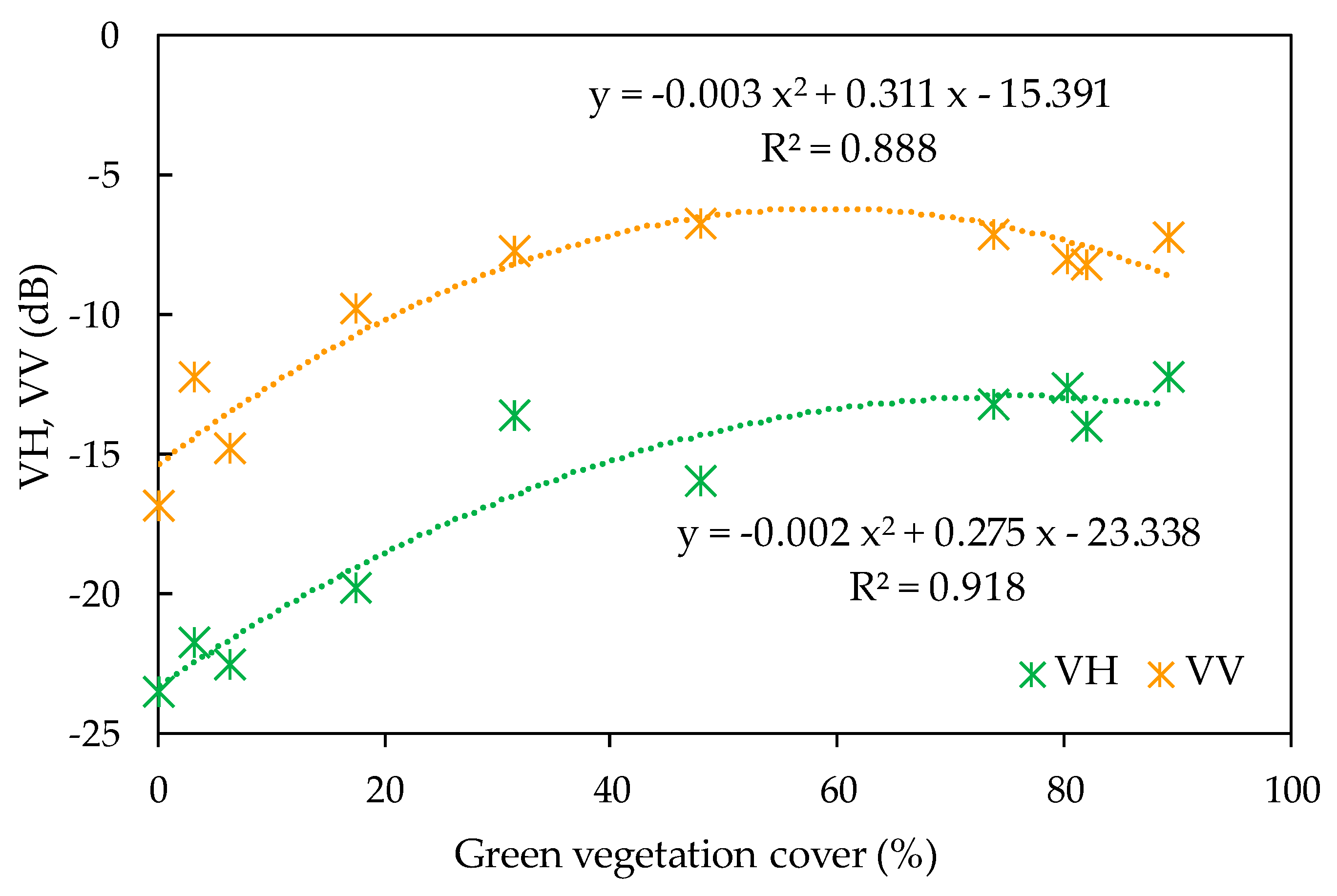
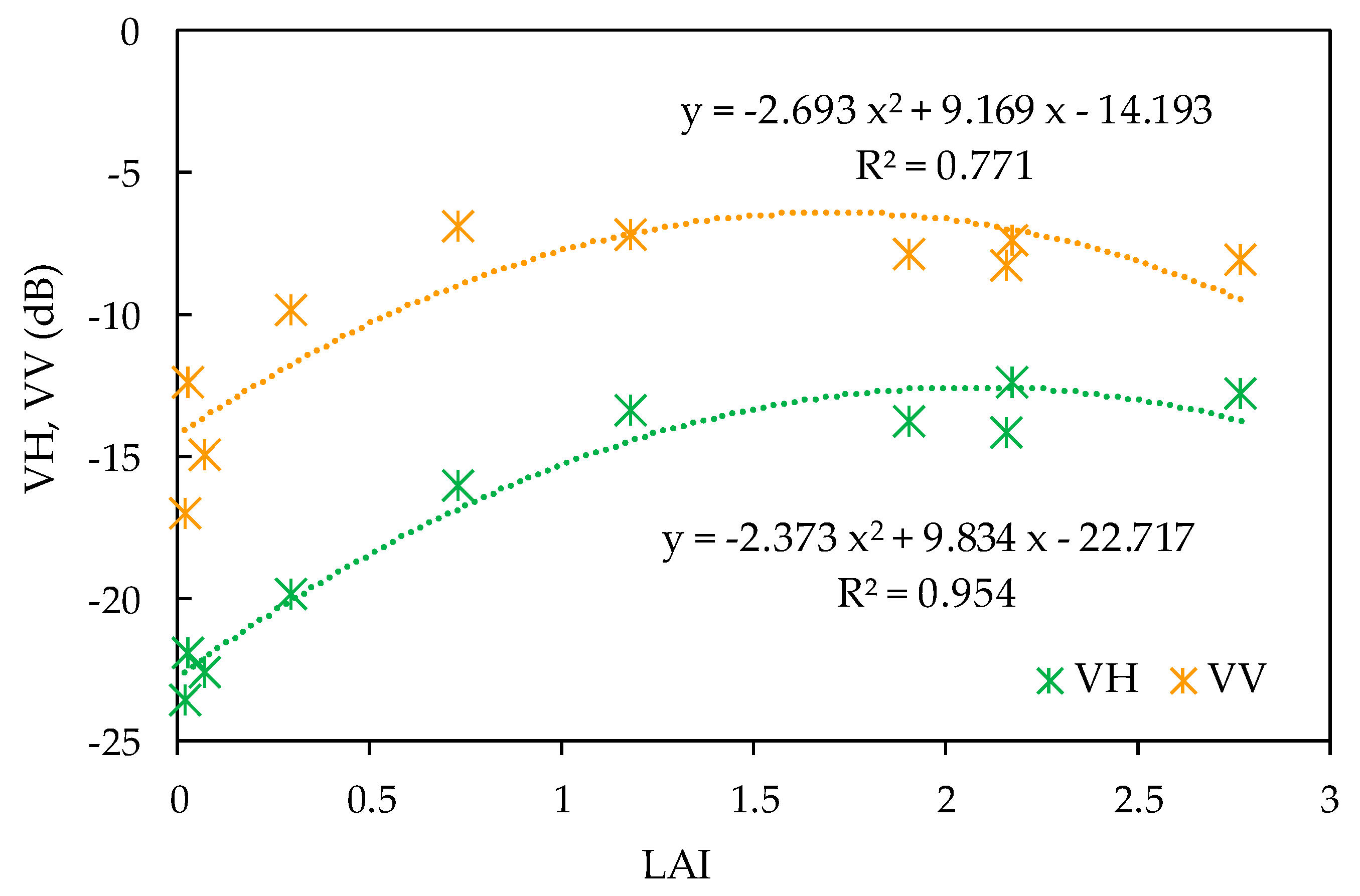
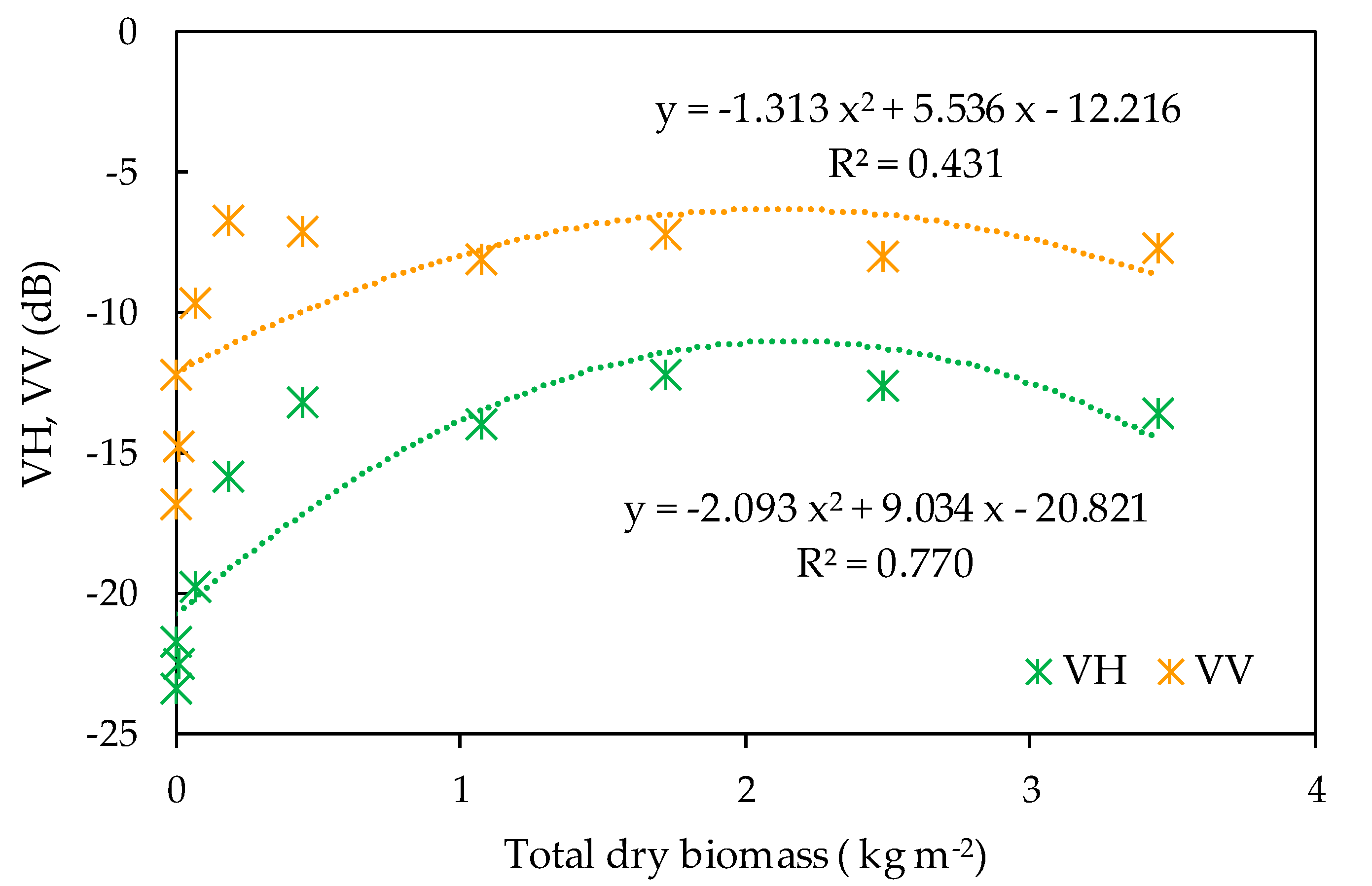
3.3. Relationship between Backscatter and Rice Biophysical Parameters Expressed with Polynomial Regression

The relationship between VH or VV and the plant biophysical parameters, with single polynomial regression lines, is shown in Figure 9, Figure 10, Figure 11 and Figure 12. Our results from the polynomial regression agree with the results reported by Chakraborty et al. [19], where they studied rice crop biophysical parameters, that is, crop height, using SAR data obtained by Radarsat. They found that polynomial relationships are the most appropriate to link plant height and SAR backscattering coefficients. They obtained coefficients of determination between backscatter and plant height, where R² = 0.694, 0.693, 0.527, and 0.947 for beam S-1, S-5, S-6, and S-7, respectively, while in our case, R² = 0.952 and 0.874 for VH and VV, respectively (Figure 9). In a similar type of study, Le Toan et al. studied the relationship between backscatter and rice crop parameters, that is, plant height and biomass, using ERS-1 data [34], demonstrating a high-performance description by polynomial regression. R² values shown in Figure 9, Figure 10, Figure 11 and Figure 12 indicate that VH is superior to VV. Compared with VV, VH backscattering coefficients have a much stronger relationship to all of the tested biophysical parameters, where plant height, green vegetation cover, and LAI versus VH had an R² greater than 0.9 (Figure 9, Figure 10 and Figure 11). Compared with these three biophysical parameters, total dry biomass had a weaker relationship to backscattering coefficients (Figure 12). Total dry biomass is constantly low during the vegetative stage, but the backscattering coefficients change significantly during the period (Figure 7D and Figure 8). In the following reproductive and ripening stages, total dry biomass increases significantly, but the backscattering coefficients values are stable. Therefore, it is difficult to correlate the total dry biomass and backscattering coefficients.

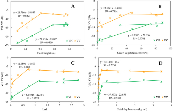
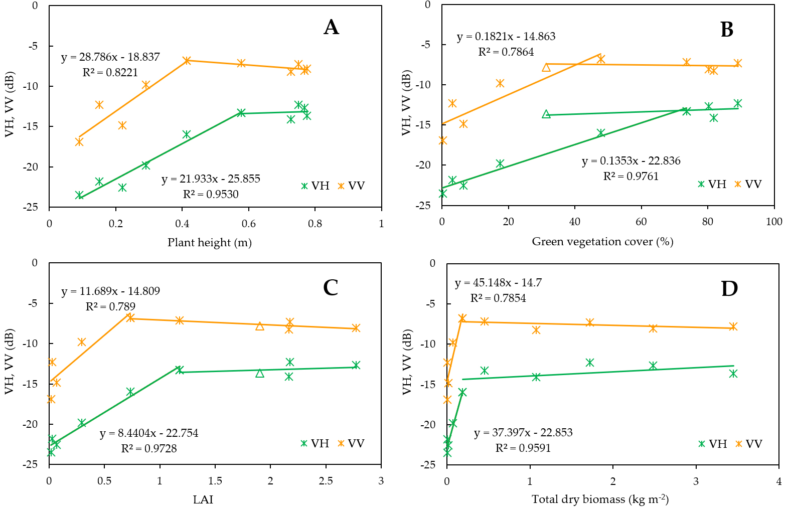
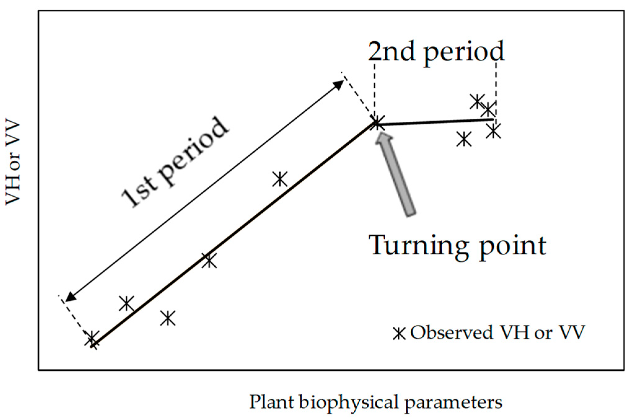
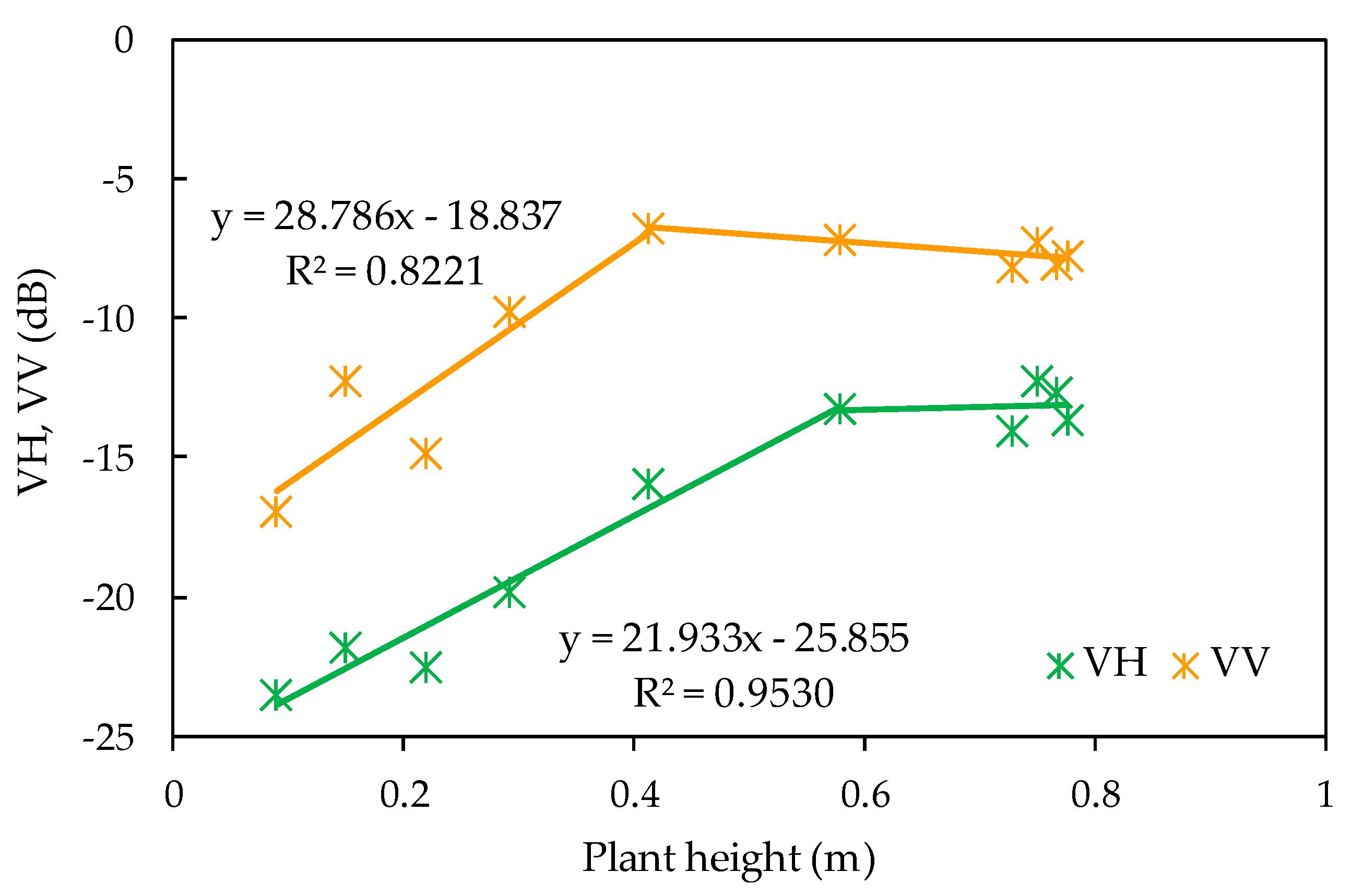
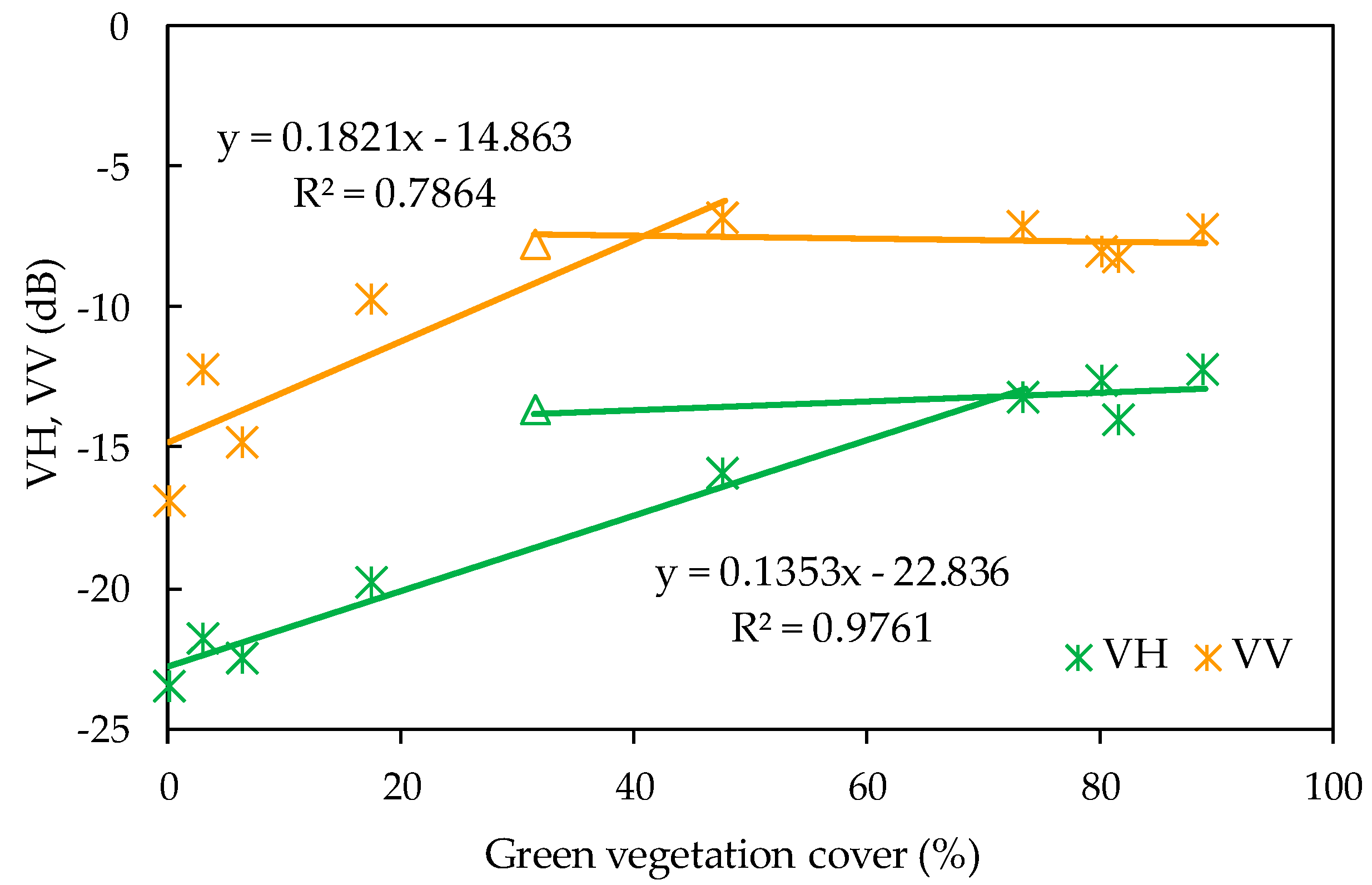
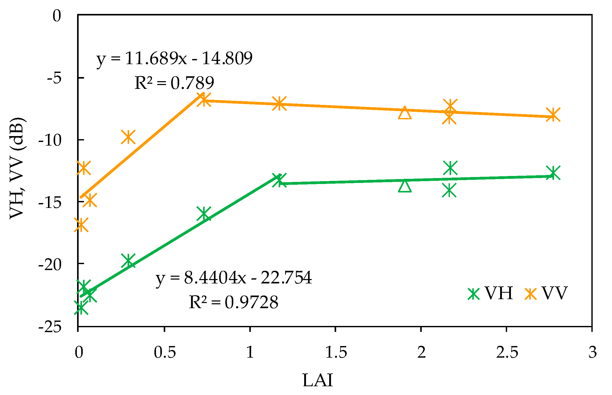
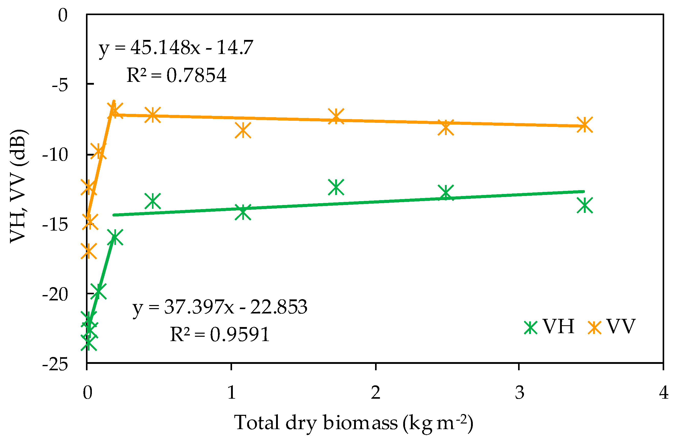
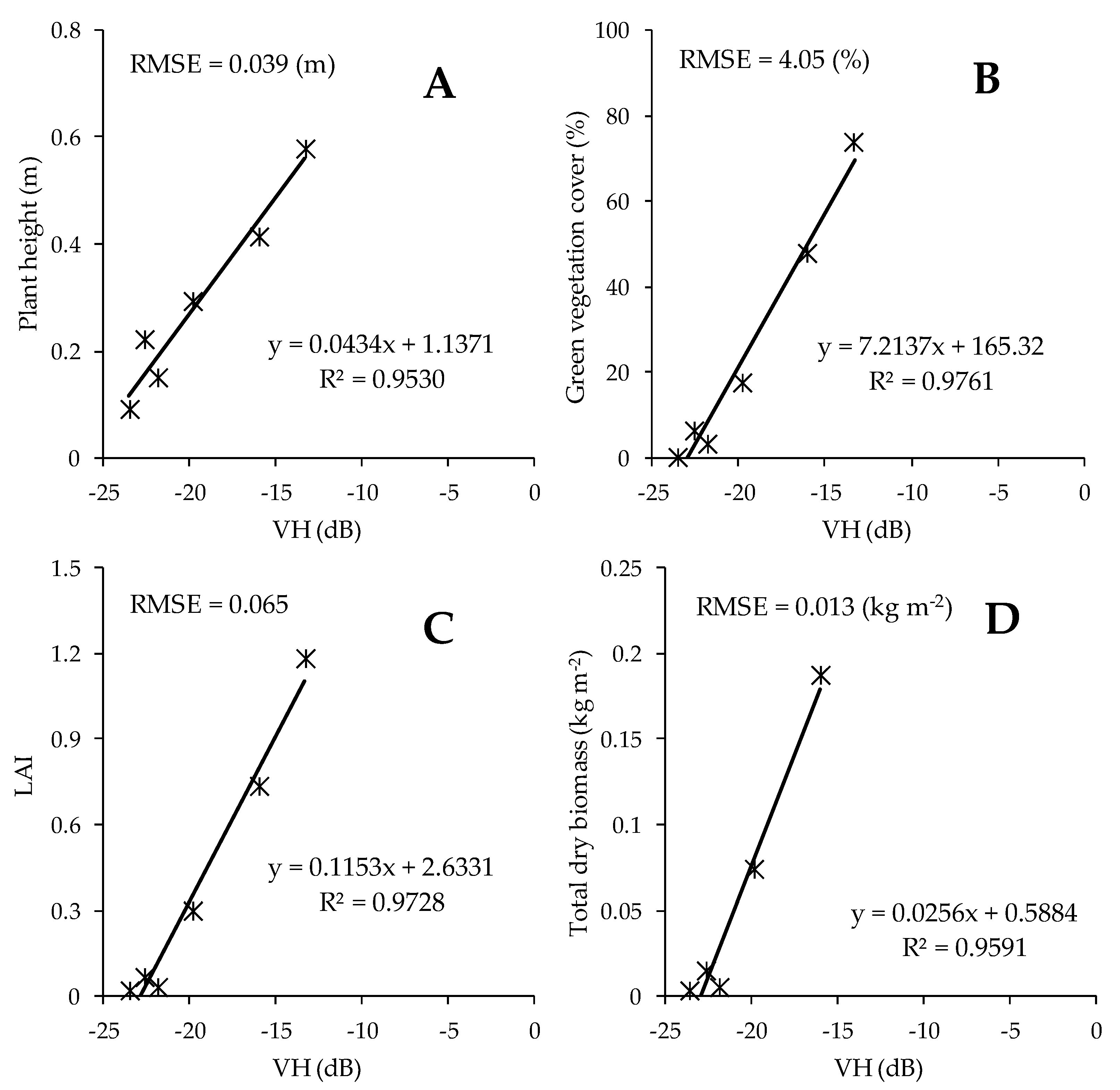
3.4. Relationship between Backscattering Coefficients and Rice Biophysical Parameters Expressed by Two Linear Regression Lines

Even though the polynomial regression reasonably expresses the relationship between backscattering coefficients and the biophysical parameters, except the total dry biomass, the polynomial approach has an operational inconvenience for rice crop monitoring by satellite SAR. The polynomial equation accepts two solutions for a specific backscattering coefficient value. For example, VH = −13 dB can either take LAI = 1.6 or 2.5 (Figure 11), which is inconvenient when estimating LAI by satellite-observed backscattering coefficients. As a unique attempt by this study, Figure 13, Figure 14, Figure 15 and Figure 16 show the relationship between VH or VV and plant biophysical parameters by a combination of two linear regression lines. The regression equations shown in the figures are for the linear regressions of the first periods, where the first period is defined in Figure 6. Data plot by triangles, appearing in Figure 14 and Figure 15, are the data for the last day of ground observation, where some reductions of green vegetation cover and LAI were confirmed by plant senescence (Figure 7B,C). Such data were treated as the data for second period.

By the analysis of R² values, the “turning point” for all combinations of biophysical parameters and VV was 48 days after transplant, which is the beginning of the reproductive stage. The turning point is later in most combinations with VH and was 60 days after transplant (the mid-reproductive stage). Compared with VV, VH has higher R² values, and has a later turning point (meaning that VH has higher tolerance to saturation), indicating that VH is superior to monitor the rice crop. The nearly horizontal regression lines in the second stages indicated that both VH and VV backscatter coefficients were saturated after passing the turning point. Further changes in biophysical parameters after the turning point cannot be described by SAR monitoring.

Table 2. Statistical summary of the linear regression lines.

Combination	First Period		Second Period
	p-Value	R2	p-Value	R2
Plant height and VH	0.01	0.953	0.834	0.017
Green vegetation cover and VH	<0.001	0.976	0.446	0.204
LAI and VH	<0.001	0.973	0.610	0.097
Total dry biomass and VH	0.04	0.959	0.314	0.249
Plant height and VV	0.034	0.822	0.061	0.626
Green vegetation cover and VV	0.045	0.786	0.698	0.041
LAI and VV	0.044	0.789	0.045	0.674
Total dry biomass and VV	0.045	0.785	0.22	0.346

shows the summary of significant test for the regression lines with the R² values of the lines. The linear regression lines are statistically significant (p-value < 0.05) for all combinations during the first period, but not in the second period (p-values > 0.05) except the combination of LAI monitored by VV (p = 0.045). In the first period, p-values are smaller (i.e., more significant) in VH than VV for all biophysical parameters, indicating that VH is superior to monitor the rice crop. Compared with the polynomial approach, the two linear regression approach better described the relationship between biophysical parameters and SAR backscattering coefficients, especially with VH. The lines visually fit well to the scatter plot, even for total dry biomass, which was difficult to describe with the polynomial line.

Figure 9, Figure 10, Figure 11, Figure 12, Figure 13, Figure 14, Figure 15 and Figure 16 show the backscattering coefficients as the y-axis, which is a typical format in similar studies. However, backscattering coefficients should be the explanatory variable and the biophysical parameters should be the objective variables when estimating plant biophysical parameters by satellite-SAR monitoring. Figure 17 shows the relationship between VH and the biophysical parameters for the first period, where the biophysical parameters are plotted as the y-axis. A caution to use with the regression equation (shown in Figure 17), for predicting plant biophysical parameters in operation, is that the minimum number of the biophysical parameters should be limited as zero, because negative numbers of these parameters do not have any physical meaning. The linear regression accurately reproduced the biophysical parameters for the first period, with a root mean square error (RMSE) = 0.039 m for plant height, 4.05% for green vegetation cover, 0.065 for LAI, and 0.013 kg m⁻² for total dry biomass. However, this approach is not applicable after about 60 days from transplant, owing to saturation of the backscattering coefficients of VH in late cultivation season. Rice crop biophysical monitoring by SAR is very effective, but only up to mid reproductive stages.

While this study demonstrated the potential and the limitation in applicability of the combination of linear regression lines, sensitivity of the calibrated constants in the estimation equation to a variation of field conditions (e.g., different field, year, region, variety of rice crop) has not been evaluated. Future study topics include the application of the suggested methodology to different years and/or locations to investigate how the relationship between SAR backscatter coefficients and the rice biophysical parameters are sensitive to the field management and yearly change of the weather condition. Enhancing the number of ground sampling is another future topic to better stabilize the data for analysis.

4. Conclusions

The objectives of this research were to study the relationship between SAR backscattering coefficients and rice crop biophysical parameters using Sentinel-1 satellite imagery, and to suggest an approach to evaluate plant biophysical parameters of rice crop using a combination of linear regression lines. Setting a study area in paddy rice fields in Miyazaki, Japan, ground measurements were conducted for plant height, green vegetation cover, LAI, and the total dry biomass of rice crop, every 12 days, simultaneously to the Sentinel-1A satellite SAR observations. Relationships between the plant biophysical parameters and SAR backscattering coefficients (VH and VV polarization) were analyzed. The results indicated that SAR backscattering coefficients linearly increase as plant biophysical parameters develop, until the “turning point,” which is 48 (VV) or 60 (VH) days after transplant. The timing corresponds to the beginning of the mid reproductive stages. During the period from transplant to the turning point, plant height, green vegetation cover, LAI, and total dry biomass were precisely described by SAR monitoring, especially with VH polarization. The performance of crop monitoring by SAR was very high during the period; RMSE in estimations of these four biophysical parameters by VH backscattering coefficients were 0.039 m for plant height, 4.05% for green vegetation cover, 0.065 for LAI, and 0.013 kg m⁻² for total dry biomass. However, backscattering coefficients saturate after the day of the turning point, and become insensitive to further developments of the plant biophysical parameters. Specifically, this research indicates that rice crop monitoring of biophysical properties by SAR is very effective, but only up to mid reproductive stages. Future study includes a sensitivity analysis of regression equations for field management.

References

1. Sasaki, T.; Ashikari, M. Rice Genomics, Genetics and Breeding; Sasaki, T., Ashikari, M., Eds.; Springer Singapore: Singapore, 2018; ISBN 978-981-10-7460-8. [Google Scholar]
2. Chen, J.; Lin, H.; Pei, Z. Application of ENVISAT ASAR data in mapping rice crop growth in Southern China. IEEE Geosci. Remote Sens. Lett. 2007, 4, 431–435. [Google Scholar] [CrossRef]
3. Liew, S.C.; Kam, S.P.; Tuong, T.P.; Chen, P.; Minh, V.Q.; Lim, H. Application of multitemporal ERS-2 synthetic aperture radar in delineating rice cropping systems in the Mekong River Delta, Vietnam. IEEE Trans. Geosci. Remote Sens. 1998, 36, 1412–1420. [Google Scholar] [CrossRef]
4. Brisco, B.; Brown, R.J.; Hirose, T.; McNairn, H.; Staenz, K. Precision agriculture and the role of remote sensing: A review. Can. J. Remote Sens. 2014, 24, 315–327. [Google Scholar] [CrossRef]
5. Torbick, N.; Chowdhury, D.; Salas, W.; Qi, J. Monitoring rice agriculture across Myanmar using time series Sentinel-1 assisted by Landsat-8 and PALSAR-2. Remote Sens. 2017, 9, 119. [Google Scholar] [CrossRef] [Green Version]
6. Shaw, D.J. Global information and early warning system. In World Food Security; Palgrave Macmillan: London, UK, 2007; pp. 163–164. [Google Scholar]
7. MARS Explorer—JRC Science Hub—European Commission. Available online: http://www.marsop.info/en/web/mars-explorer/home (accessed on 22 October 2019).
8. CropMonitor. Available online: http://www.cropmonitor.co.uk/ (accessed on 22 October 2019).
9. CropWatch. Available online: http://cloud.cropwatch.com.cn/ (accessed on 22 October 2019).
10. UN-SPIDER (United Nations Platform for Space-based Information for Disaster Management and Emergency Response). Available online: http://www.unoosa.org/oosa/en/ourwork/un-spider/index.html (accessed on 22 October 2019).
11. FEWS NET (Famine Early Warning Systems Network). Available online: https://fews.net/ (accessed on 22 October 2019).
12. Torbick, N.; Salas, W. Mapping agricultural wetlands in the Sacramento Valley, USA with satellite remote sensing. Wetl. Ecol. Manag. 2015, 23, 79–94. [Google Scholar] [CrossRef]
13. Zhou, Y.; Xiao, X.; Qin, Y.; Dong, J.; Zhang, G.; Kou, W.; Jin, C.; Wang, J.; Li, X. Mapping paddy rice planting area in rice-wetland coexistent areas through analysis of Landsat 8 OLI and MODIS images. Int. J. Appl. Earth Obs. Geoinf. 2016, 46, 1–12. [Google Scholar] [CrossRef] [Green Version]
14. Huke, R.E.; Huke, E.H. Rice Area by Type of Culture: South, Southeast, and East Asia. A Review and Updated Data Base; IRRI: Manila, Philippines, 1997; ISBN 9712200922. [Google Scholar]
15. Nelson, A.; Setiyono, T.; Rala, A.; Quicho, E.; Raviz, J.; Abonete, P.; Maunahan, A.; Garcia, C.; Bhatti, H.; Villano, L.; et al. Towards an operational SAR-based rice monitoring system in Asia: Examples from 13 demonstration sites across Asia in the RIICE project. Remote Sens. 2014, 6, 10773–10812. [Google Scholar] [CrossRef] [Green Version]
16. Moreira, A.; Prats-Iraola, P.; Younis, M.; Krieger, G.; Hajnsek, I.; Papathanassiou, K.P. A tutorial on synthetic aperture radar. IEEE Geosci. Remote Sens. Mag. 2013, 1, 6–43. [Google Scholar] [CrossRef] [Green Version]
17. Chen, C.; Mcnairn, H. A neural network integrated approach for rice crop monitoring. Int. J. Remote Sens. 2006, 27, 1367–1393. [Google Scholar] [CrossRef]
18. Bouvet, A.; Le Toan, T.; Lam-Dao, N. Monitoring of the rice cropping system in the Mekong Delta using ENVISAT/ASAR dual polarization data. IEEE Trans. Geosci. Remote Sens. 2009, 47, 517–526. [Google Scholar] [CrossRef] [Green Version]
19. Chakraborty, M.; Manjunath, K.R.; Panigrahy, S.; Kundu, N.; Parihar, J.S. Rice crop parameter retrieval using multi-temporal, multi-incidence angle Radarsat SAR data. ISPRS J. Photogramm. Remote Sens. 2005, 59, 310–322. [Google Scholar] [CrossRef]
20. Kurosu, T.; Fujita, M.; Chiba, K. Monitoring of rice crop growth from space using the ERS-1 C-band SAR. IEEE Trans. Geosci. Remote Sens. 1995, 33, 1092–1096. [Google Scholar] [CrossRef]
21. Nguyen, D.B.; Gruber, A.; Wagner, W. Mapping rice extent and cropping scheme in the Mekong Delta using Sentinel-1A data. Remote Sens. Lett. 2016, 7, 1209–1218. [Google Scholar] [CrossRef]
22. Rucci, A.; Ferretti, A.; Guarnieri, A.M.; Rocca, F. Sentinel 1 SAR interferometry applications: The outlook for sub millimeter measurements. Remote Sens. Environ. 2012, 120, 156–163. [Google Scholar] [CrossRef]
23. Le Toan, T.; Laur, H.; Mougin, E.; Lopes, A. Multitemporal and dual-polarization observations of agricultural vegetation covers by X-band SAR images. IEEE Trans. Geosci. Remote Sens. 1989, 27, 709–718. [Google Scholar] [CrossRef]
24. Mansaray, L.R.; Zhang, D.; Zhou, Z.; Huang, J. Evaluating the potential of temporal Sentinel-1A data for paddy rice discrimination at local scales. Remote Sens. Lett. 2017, 8, 967–976. [Google Scholar] [CrossRef]
25. Wu, F.; Wang, C.; Zhang, H.; Zhang, B.; Tang, Y. Rice crop monitoring in South China with RADARSAT-2 quad-polarization SAR data. IEEE Geosci. Remote Sens. Lett. 2011, 8, 196–200. [Google Scholar] [CrossRef]
26. Bourbigot, M.; Johnsen, H.; Piantanida, R. Sentinel-1 Product Definition. Document Number: S1-RS-MDA-52-7440 S-1 MPC Nomenclature: DI-MPC-PB, S-1 MPC Reference: MPC-0239. Available online: https://sentinel.esa.int/documents/247904/1877131/Sentinel-1-Product-Definition (accessed on 10 October 2019).
27. Atwood, D.K.; Small, D.; Gens, R. Improving PolSAR land cover classification with radiometric correction of the coherency matrix. IEEE J. Sel. Top. Appl. Earth Obs. Remote Sens. 2012, 5, 848–856. [Google Scholar] [CrossRef]
28. Small, D. Flattening gamma: Radiometric terrain correction for SAR imagery. IEEE Trans. Geosci. Remote Sens. 2011, 49, 3081–3093. [Google Scholar] [CrossRef]
29. Small, D.; Miranda, N.; Meier, E. A revised radiometric normalisation standard for SAR. In Proceedings of the 2009 IEEE International on Geoscience and Remote Sensing Symposium (IGARSS), Cape Town, South Africa, 12–17 July 2009; pp. 566–569. [Google Scholar]
30. Small, D.; Jehle, M.; Schubert, A.; Meier, E. Accurate geometric correction for normalisation of PALSAR radiometry. In Proceedings of the ALOS 2008 Symposium, Rhodes, Greece, 3–7 November 2008; p. 7. [Google Scholar]
31. Patrignani, A.; Ochsner, T.E. Canopeo: A powerful new tool for measuring fractional green canopy cover. Agron. J. 2015, 107, 2312–2320. [Google Scholar] [CrossRef] [Green Version]
32. Abramoff, M.D.; Magalhães, P.J.; Ram, S.J. Image processing with ImageJ. Biophotonics Int. 2004, 11, 36–42. [Google Scholar]
33. Shao, Y.; Fan, X.; Liu, H.; Xiao, J.; Ross, S.; Brisco, B.; Brown, R.; Staples, G. Rice monitoring and production estimation using multitemporal RADARSAT. Remote Sens. Environ. 2001, 76, 310–325. [Google Scholar] [CrossRef]
34. Le Toan, T.; Ribbes, F.; Wang, L.F.; Floury, N.; Ding, K.H.; Kong, J.A.; Fujita, M.; Kurosu, T. Rice crop mapping and monitoring using ERS-1 data based on experiment and modeling results. IEEE Trans. Geosci. Remote Sens. 1997, 35, 41–56. [Google Scholar] [CrossRef]
Figure 1. Location of study site.
Remotesensing 12 00189 g001
Figure 2. Monthly average air temperature and rainfall in Miyazaki, Japan.
Remotesensing 12 00189 g002
Figure 3. Rice crop growth stages in the study area in 2018.
Remotesensing 12 00189 g003
Figure 4. Location of sampling pixels in the study field.
Remotesensing 12 00189 g004
Figure 5. Photos of study field during the study period.
Remotesensing 12 00189 g005
Figure 6. Diagram expressing the relationship between plant biophysical parameters and synthetic aperture radar (SAR) backscatter signals using two linear regression lines. VH, vertical transmitting, horizontal receiving; VV, vertical transmitting, vertical receiving.
Remotesensing 12 00189 g006
Figure 7. Ground measured temporal variations in (A) plant height, (B) green vegetation cover, (C) leaf area index (LAI), and (D) total dry biomass, after transplantation.
Remotesensing 12 00189 g007
Figure 8. Temporal variation in SAR backscattering coefficients after transplantation.
Remotesensing 12 00189 g008
Figure 9. Backscattering coefficients as a function of plant height, expressed by polynomial regressions.
Remotesensing 12 00189 g009
Figure 10. Backscattering coefficients as a function of green vegetation cover, expressed by polynomial regressions.
Remotesensing 12 00189 g010
Figure 11. Backscattering coefficients as a function of LAI, expressed by polynomial regressions.
Remotesensing 12 00189 g011
Figure 12. Backscattering coefficients as a function of total dry biomass, expressed by polynomial regressions.
Remotesensing 12 00189 g012
Figure 13. Backscattering coefficients as a function of plant height, expressed by a combination of two linear regressions.
Remotesensing 12 00189 g013
Figure 14. Backscattering coefficients as a function of green vegetation cover, expressed by a combination of two linear regressions.
Remotesensing 12 00189 g014
Figure 15. Backscattering coefficients as a function of LAI, expressed by a combination of two linear regressions.
Remotesensing 12 00189 g015
Figure 16. Backscattering coefficients as a function of total dry biomass, expressed by a combination of two linear regressions.
Remotesensing 12 00189 g016
Figure 17. Plant biophysical parameters (A); plant height, (B); green vegetation cover, (C); leaf area index, (D); total dry biomass) expressed by VH backscattering coefficients for the first period before the turning point. RMSE, root mean square error.
Remotesensing 12 00189 g017