Article

Predicting Carbon Accumulation in Temperate Forests of Ontario, Canada Using a LiDAR-Initialized Growth-and-Yield Model

by
Paulina T. Marczak
1,*,
Karin Y. Van Ewijk
1,
Paul M. Treitz
1,
Neal A. Scott
1 and
Donald C.E. Robinson
2
1
Department of Geography and Planning, Queen’s University, Kingston, ON K7L 3N6, Canada
2
ESSA Technologies, Vancouver, BC V6J 5C6, Canada
*
Author to whom correspondence should be addressed.
Submission received: 2 December 2019 / Revised: 23 December 2019 / Accepted: 3 January 2020 / Published: 6 January 2020
(This article belongs to the Special Issue Remote Sensing of Forest Growth in a Changing Climate)

Abstract

:
Climate warming has led to an urgent need for improved estimates of carbon accumulation in uneven-aged, mixed temperate forests, where high uncertainty remains. We investigated the feasibility of using LiDAR-derived forest attributes to initialize a growth and yield (G&Y) model in complex stands at the Petawawa Research Forest (PRF) in eastern Ontario, Canada; i.e., can G&Y models based on LiDAR provide accurate predictions of aboveground carbon accumulation in complex forests compared to traditional inventory-based estimates? Applying a local G&Y model, we forecasted aboveground carbon stock (tons/ha) and accumulation (tons/ha/yr) using recurring plot measurements from 2012–2016, FVS1. We applied statistical predictors derived from LiDAR to predict stem density (SD), stem diameter distribution (SDD), and basal area distribution (BA_dist). These data, along with measured species abundance, were used to initialize a second model (FVS2). A third model was tested using LiDAR-initialized tree lists and photo-interpreted estimates of species abundance (i.e., FVS3). The carbon stock projections for 2016 from the inventory-based G&Y model) were equivalent to validation carbon stocks measured in 2016 at all size-class levels (p < 0.05), while LiDAR-based G&Y models were not. None of the models were equivalent to validation data for accumulation (p > 0.05). At the plot level, LiDAR-based predictions of carbon accumulation over a nine-year period did not differ when using either inventory or photo-interpreted species (p < 0.05). Using a constant mortality rate, we also found statistical equivalency of inventory and photo-interpreted accumulation models for all size classes ≥17 cm. These results suggest that more precise information is needed on tree characteristics than we could derive from LiDAR, but that plot-level species information is not as critical for predictions of carbon accumulation in mixed-species forests. Further work is needed on the use of LiDAR to quantify stand properties before this technique can be used to replace recurring plot measurements to quantify carbon accumulation.

Graphical Abstract

1. Introduction

Forests play a key role in the global carbon cycle, storing 80% of all terrestrial aboveground carbon [1] and contribute substantially to the total annual global terrestrial carbon sink (3.0 ± 0.8 GtC/yr) [2] with recent estimates placing the net global forest sink at 1.1 ± 0.8 GtC/yr [3]. Sustainable forest management (SFM) practices could be developed to enhance rates of carbon sequestration in forests (e.g., [4]). To account for the impact of SFM practices on rates of carbon storage over large areas, spatially comprehensive techniques are needed to quantify carbon stocks (tons/ha) and predict carbon stock changes (tons/ha/yr). This would allow forest managers to (i) make more informed management decisions and; (ii) enhance the use of forests to limit the rate of climate warming [5].
Predictions of aboveground forest carbon accumulation (i.e., tree growth) are often made by applying statistical models of forest growth and yield (G&Y) to plot-level inventory data [6]. The key challenge is the extrapolation of plot-level data over larger areas. Plot-scale forest inventories often have limited point sampling, high cost, and limited personnel [5,7]. These G&Y models may require inputs of tree-level diameter-at-breast height (DBH), species, site quality, and other attributes to project future carbon accumulation [8]. To apply G&Y models over large areas, remote sensing methods would be required to collect spatially-explicit (i.e., “wall-to-wall”) data that can be used to initialize G&Y models. Spatially comprehensive estimates of biomass and growth would support SFM, especially in complex forests with multiple tree ages (i.e., size classes) and species [9].
Light detection and ranging (LiDAR; also referred to as airborne laser scanning; ALS) is an active remote sensing system that generates a 3-D point cloud from which statistical metrics defining vertical and horizontal forest structure are derived [10,11]. In this discrete return system, a pulse of laser light travels to the object, where the time of travel to and from the object for each individual laser pulse is recorded to determine the distance, referred to as pulsed ranging [12]. A discrete-return sensor can transmit up to five returns; when a laser pulse hits the bare ground or a dense object, only a single return is recorded [11,13]. Conversely, when the pulse travels through a forest canopy, some component energy can intercept various components of the understory, as well as the ground, resulting in multiple returns [11]. The metrics, which statistically describe the point cloud (e.g., percentiles, density) can be used as independent variables to predict stem diameter distribution (SDD; i.e., the number of stems/ha across a set of diameter size classes), stem density (SD; stems/ha for a given plot), species abundance, and other attributes needed to initialize G&Y models [9,13,14]. Studies that predict SDD from LiDAR have been limited; this can be partially attributed to the low accuracy of predicting multiple response variables, which complicate model calibration and validation [14]. SDD is thus often weighted by basal area (BA); i.e., the cross-sectional area of a tree at breast height across a hectare, in m2/ha) due to the intrinsic quadratic relationship between DBH and BA [15]; BA distribution (BA_dist) (i.e., the value of the summed individual-tree BA across a hectare in a distributed range, e.g., size classes, in m2/ha), gives greater importance to larger trees and improves predictions, thus is often used in SDD studies [16,17]. Previous studies have initialized local G&Y models using LiDAR-predicted variables to evaluate BA_dist as a proxy for growth [5], or map present aboveground carbon density using predictions of SDD [18]. Others have used process-based modelling to evaluate its effectiveness in single-species forests/plantations for BA_dist growth [19] and biomass [20]. Zhang et al. (2018) [21] used repeat LiDAR surveys to calibrate biomass change. Thus, the application of LiDAR to quantify stand characteristics for the initialization of G&Y models has the potential for predicting carbon accumulation in uneven-aged mixedwood temperate forests.
Area-based approaches (ABAs) to quantify SDD and BA_dist using LiDAR metrics include both parametric and non-parametric techniques. Parametric techniques assume that the data conforms to a given probability density function (PDF; [22]) such as the Weibull distribution, which has been used extensively to predict SDD and BA_dist [23,24]. Some have alluded to predicting future growth based on moderate success predicting SDD and other stand attributes across a landscape using parametric approaches (e.g., [18]). However, modelling of SDD and BA_dist in complex forests has proven to be more challenging. As a result, non-parametric techniques such as k-nearest neighbours (k-NN) and random forests (RF) are becoming increasingly popular [5,8,25,26]. Non-parametric techniques offer the advantage of identifying important variables using variable reduction techniques and eliminating those variables with high collinearity, thus promoting them for LiDAR-based applications in complex forests [14,27].
To date, the application of non-parametric approaches to create tree lists and project G&Y models for carbon accumulation has been limited, and, to the best of our knowledge, virtually non-existent in complex forests with mixed species and age structures. For the purposes of this study, we defined tree lists as lists of species-assigned stem diameters for the number of trees in a stand, excluding site class or height. A previous study used k-NN imputation to parameterize the Forest Vegetation Simulator (FVS; [28]) over a large forested area in Oregon, finding that k-NN exhibited higher accuracy for larger trees and concluded that LiDAR could be used for spatially explicit BA_dist projections [5]. Tompalski et al. (2018) [29] used an ABA approach to find the best matching yield curves compared to those generated by a locally parameterized model. Others report predictions of single-tree attributes including SDD, but do not compare projections of future growth (e.g., [14,30]). Many studies that have used the RF non-parametric algorithm found it stronger at predicting forest attributes than other non-parametric approaches, including k-NN [14,30,31], however, there remains no consensus on a preferred model across conditions [8]. Application of RF for predicting forest attributes in complex stands (i.e., mixedwood, uneven-aged) is increasing given it alleviates several challenges associated with parametric techniques, including: (i) the need for significant a priori knowledge to properly parameterize models; (ii) collinearity between predictors; and (iii) overfitting when a large number of predictor variables are used [14]. Whereas parametric models must be highly parameterized to predict complex SDDs and often require forest type stratification to improve model accuracy, RF is not constrained by these requirements [24,31,32,33]. Predicting species abundance, a requirement in initializing many G&Y models, has also proved to be challenging in mixedwood forests due to increased structural complexity, coupled with the challenges of accurately normalizing LiDAR strength of return (i.e., intensity [34,35]), although advances have been made (e.g., [36,37]). However, the error associated with an imprecise or inaccurate characterization of species abundance on growth estimates remains unclear, as studies do not typically compare any potential changes in accuracy using inventory-derived species abundance compared to predictions from LiDAR for G&Y models (e.g., [5,38,39]).
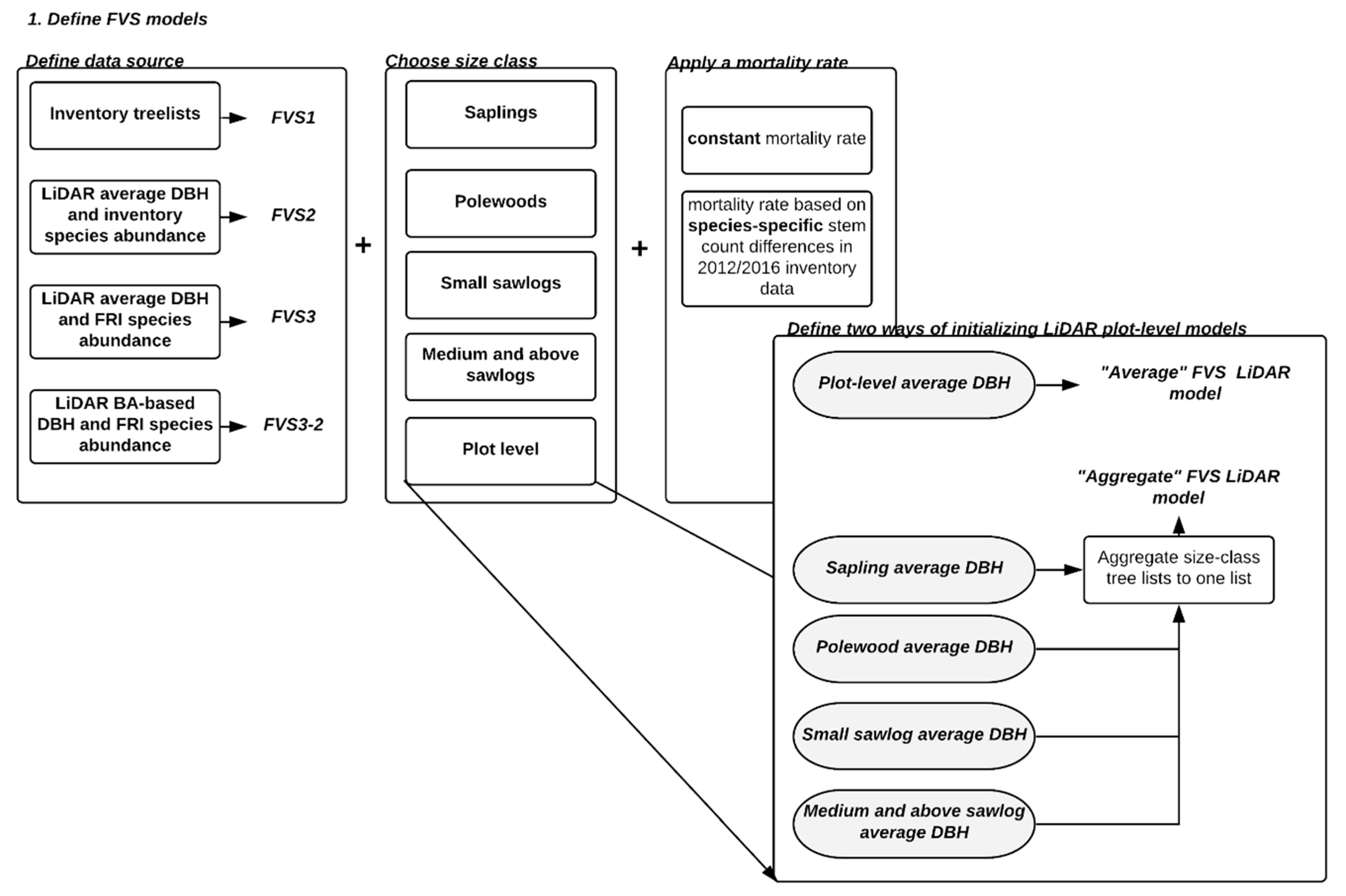
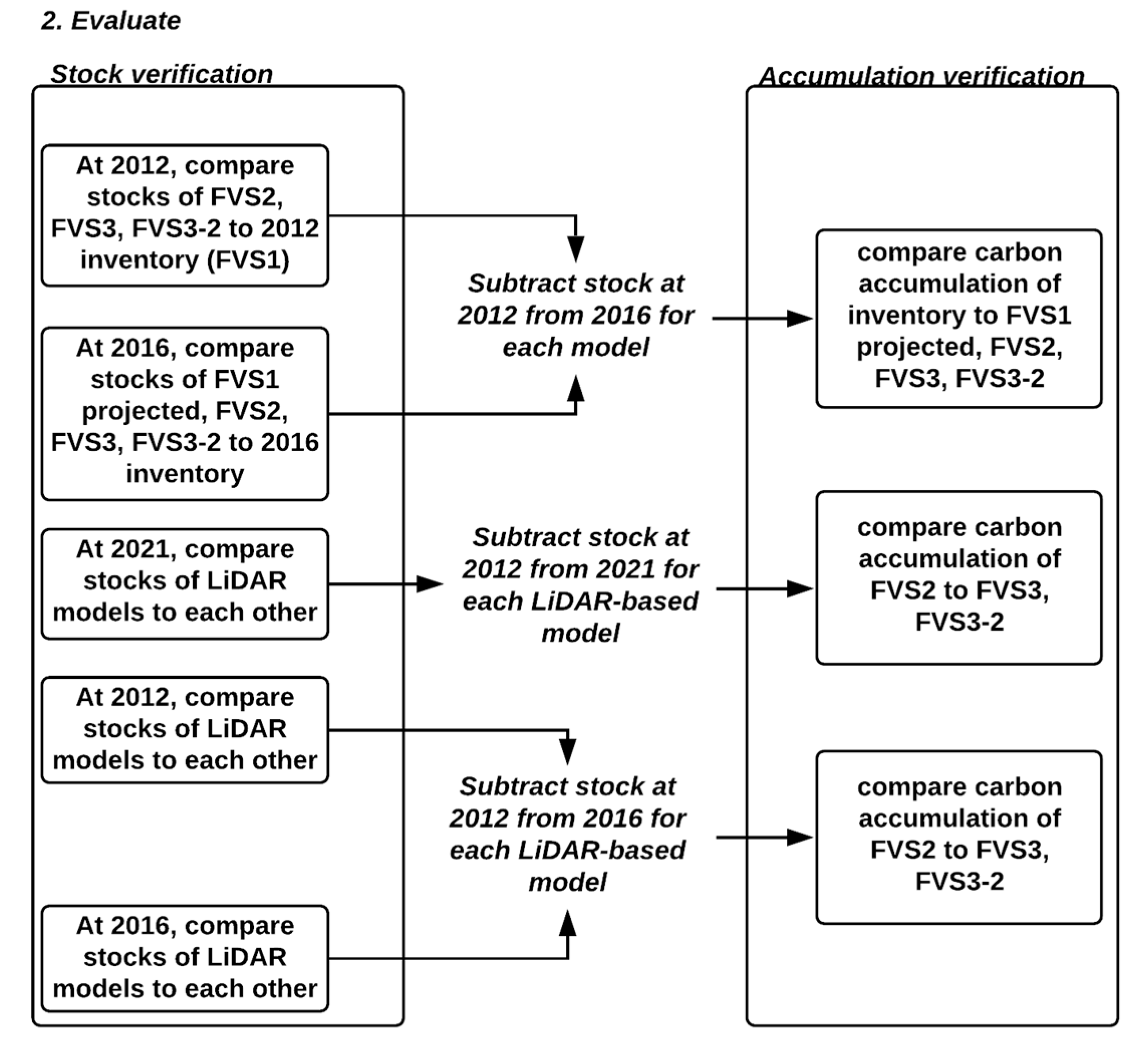
In general, predicting tree growth, specifically using ABAs, has a number of challenges due to the need to disaggregate size class-level predictions to tree-level, apply this across a larger area, and then impute or otherwise obtain species abundance. In this study, we tested the initialization of a LiDAR-derived G&Y model using average diameter tree lists combined with a suite of G&Y model specifications and tests of different approaches to quantify species abundance. We used estimates of BA_dist and SDD/SD to initialize an individual tree-based G&Y model (i.e., FVSOntario) to investigate the feasibility of forecasting carbon accumulation (i.e., the difference in carbon stock between years) in an uneven-aged, mixedwood forest (i.e., the Great Lakes - St. Lawrence forest). Our objectives were: (1) initialize a baseline G&Y model (i.e., FVS1) using plot-based diameter-at-breast-height (DBH) measures and species abundance data; (2) initialize a second G&Y model (i.e., FVS2) based on LiDAR-derived size-class DBH estimates and plot-based species abundance data; (3) initialize a third model (i.e., FVS3) using LiDAR-derived size-class DBH estimates and species abundance data inferred from the Forest Resource Inventory (FRI); (4) initialize a fourth model using BA_dist and median size-class range values to evaluate the effect of modelling without SDD (i.e., FVS3-2), and (5) compare predicted carbon accumulation for the different models to inventory-based estimates of carbon accumulation. We compared stocks at model initialization to 2012 inventory validation data (i.e., FVS1), projected stocks for all the models after a four-year simulation to 2016 inventory validation data, and further compared LiDAR model outputs at 2021.

2. Materials and Methods

2.1. Overview

For Objective 1, size class bins were defined as trees with DBH ranging from: 8–17 cm (saplings), 17–26 cm (polewoods), 26–38 cm (small sawlogs), and 38 cm and above (medium and above sawlogs). The number of individuals per size-class and plot-level tree lists (by species) were extracted from 2012/13 inventory DBH and species abundance data. For FVS2 (LiDAR-initialized tree lists and inventory-based species abundance), input variables (i.e., SDD, SD, and BA_dist) were predicted from 2012 LiDAR data using a non-parametric algorithm (i.e., RF, [40] and independently optimized predictor variables. To obtain tree lists, we divided estimates of BA_dist by SD (plot-level) or SDD (size-class level) to obtain average diameter and number of stems per plot, combined with species abundance from inventory measures. For Objective 3 (FVS3; LiDAR-initialized tree lists and FRI species abundance), LiDAR-based DBH (FVS2) was combined with photo-interpreted FRI-based species abundance and used to create input tree lists. For objective 4, determining the sensitivity of precise SDD predictions on model performance was tested by using mid-range DBH values for each size class to construct tree lists, in conjunction with predicted BA_dist for estimates of SDD and FRI-based species abundance (i.e., FVS3-2). Each model was then projected forward for four years to predict carbon stocks in 2016, and accumulation (measured as the difference between 2012 and 2016 carbon stocks). Finally, for Objective 5, we evaluated equivalency in accumulation and stock at multiple times using a regression-based equivalence test (i.e., the Robinson test, [41]). For carbon stocks, we evaluated the inventory-based projections against LiDAR-based models for 2012 and 2016, then we compared inventory and LiDAR-based projections to the 2016 inventory measures of carbon stock. For accumulation at the 2016 mark, we compared all projected models to accumulation derived from field data (i.e., field-measured tree list data converted to differences in carbon stock using the FVSOntario model between 2012–2016). Measures of species influence on carbon accumulation (i.e., significant differences between FVS2 and FVS3/FVS3-2) were evaluated for 2016 and 2021 using the same regression-based equivalence test. Lastly, the same test was applied for carbon accumulation and carbon stocks at 2021 (i.e., year nine) to determine if there were any longer-term stabilization effects on G&Y model predictions.

2.2. Study Area

The Petawawa Research Forest (PRF; 45°59′52.0″N, 77°25′39.6″W) is the older of two National Research Forests in Canada (Figure 1) [42]. PRF was established in 1918 to experiment with forest management practices for the Great Lakes - St. Lawrence Forest Region (GLSL). Located in eastern Ontario, it is 100 km2 in size and has mean annual precipitation and temperature of 859 mm and 5.6 °C, respectively [43]. The area lies on the lower reaches of the Precambrian Shield and is strongly influenced by glaciation and post-glacial outwashing, ranging in elevation from 140 to 280 m above sea level. The terrain is one of sandy plains; imposing hills and shallow, sandy soils, as well as bedrock outcrops; or gently rolling hills and deep loamy sand with boulders [44].
The GLSL is considered a transition zone between the northern boreal forests and southern deciduous forests [45]. The GLSL region experiences natural disturbances such as fire and downbursts/windthrow at an intermediate frequency. Other disturbances impacting forest structure include land-use change, insect outbreaks and fire suppression [45]. Percentage species composition at PRF include 32% white pine (P. strobus), 23% trembling aspen (P. tremuloides), 11% oak (Quercus spp.), 10% red pine (P. resinosa), 8% white birch (B. papyrifera), 5% maple (Acer spp.), 5% white spruce (P. glauca), 4% other conifers, and 2% other hardwoods [45,46]. Various silvicultural practices, including shelterwood harvesting, thinning, competition control (i.e., removal of excess trees), tree planting and scarification regeneration also influence present and future forest stand structure in parts of the forest [45,47].

2.3. FVSOntario

Forest Vegetation Simulator Ontario (FVSOntario; version 3.03.0006) is an empirical, single-tree, G&Y model parameterized for the climate and species of Ontario [48,49]. In the 1990s, suitable G&Y models were being considered for Ontario’s G&Y Program that would predict tree and stand growth better than traditional stand tables (i.e., [50]). The Forest Vegetation Simulator (FVS, [28]) was identified as a potential fit as it was able to account for a range of silvicultural treatments, species, and forest conditions; while meeting additional criteria as outlined in Woods and Robinson [49]. Results of the model evaluation of the FVS US Lake States (LS) variant indicated poor representation of growth for Ontario-specific scenarios [51]. FVSOntario was consequently developed based on multiple calibrations and validation efforts within the Boreal and Great Lakes - St. Lawrence forest regions in combination with the British Columbia variant (PrognosisBC) user interface [48,49,52].
FVSOntario contains an extension based on the US Fire and Fuels Extension (FFE, [53]) that uses individual tree lists as input and converts DBH measurements to estimates of carbon stock (metric tons/ha) using species-specific biomass conversion equations developed by Jenkins et al. (2003) [54]. This process was automated using a batch script that ran the FFE extension (i.e., the carbon submodel) used to calculate estimates of carbon stocks [55].

2.4. Field Data Collection

Inventory BA_dist and SD/SDD were derived from tree mensuration data for the size classes at the plot level, with summary statistics shown in Table 1. These data were collected for 75 circular plots (radius = 14.1 m; area = 625 m2) during the summers of 2012/2013 with re-measurement in 2016/2017 as part of this study [56,57]. Plots were selected using a stratified random sampling design; i.e., stands were selected randomly within 15 previously identified forest type strata. Plot centre locations were recorded using an SX Blue II GPS (UTM NAD83 Zone 18). Mensuration data were collected for all trees with DBH ≥ 8 cm whose centres were within the radius of the plot. Plot-level data included overall stand description (coniferous plantation, natural-deciduous canopy, natural-pine dominated canopy or natural-mixed complex canopy), origin (natural/planted), and development stage/canopy layering (stem exclusion, understory re-initiation, and old-growth). Tree-level data included DBH, species, status (live, dead, live veteran, or removed), origin (natural, planted, layering, coppice, or unknown), crown class (intermediate, co-dominant, dominant, emergent/veteran, suppressed, and anomaly), health class (healthy, minor defoliation, major defoliation, or complete defoliation), tree height for a subset of trees (height to live foliage and total tree), and decay class (1-branches still present, 5-bark completely off and no branches) for standing dead trees. The base of the live crown and total tree heights were recorded for a selection of dominant and co-dominant species using a Vertex™ hypsometer (Långsele, Sweden). Each tree in the resulting calibration data (i.e., inventory tree lists used to initialize FVS1) was then manually inspected for abnormal growth patterns. A small number of trees had a negative diameter increment in our data, however, these decreases were only attributed to dying or decayed trees and were thus included in measurements [58].

2.5. LiDAR Data Collection and Processing

LiDAR data were collected by Leading Edge Geomatics (Oromocto, NB) on 17–20 August 2012 using the Riegl Q680i sensor with a horizontal accuracy of ~0.18 m RMSE over an average flying height of 725 m a.g.l. The sensor collected data in the shortwave infrared (SWIR; 1550 nm) and possessed an average sampling density of 11.9 pulses/m2. The LiDAR data were first height-normalized using the vendor-provided 0.5 m spatial resolution digital elevation model (DEM) and the open-access Fusion software package v.3.7 [59].
A standard suite of predictive metrics describing height and intensity was generated for each of the 75 plots using the rLiDAR package in R [60,61]. Based on all returns, metrics included the proportion of first and all returns, percentiles, statistical descriptors of central tendency for height and intensity (e.g., mean, mode), spread (e.g., skewness, kurtosis), and descriptors of canopy versus non-canopy hits. Intensity-based metrics were included to enhance the potential for characterizing SDD [14]. Typically, intensity normalization requires a priori knowledge of return-scale observed range [14,62]. Although intensity could not be normalized as range information was not provided by the vendor, previous studies have suggested non-normalized intensity metrics may be useful predictors in modelling SDD [14], although normalization could improve predictive accuracy ([63,64] as cited in [14]). Following the recommendation of White et al. (2013) [11], all metrics were generated using a 1.37 m minimum height threshold (i.e., the minht parameter). Returns below this threshold were excluded. A minimum canopy threshold of 2 m was also set to represent the lower portion of the canopy for canopy-specific metrics (i.e., the above parameter; [65]).

2.6. Growth Modelling

2.6.1. SDD, SD, and BA_dist Prediction

Individual tree measurements of DBH were placed into discrete size classes (i.e., SDD), similar to the operational forest management classes as outlined in Shang et al. (2017) [14] (Table 2). Prediction within these size classes provides relevant harvesting information to inform forest management strategies. The large and extra-large sawlog classes were grouped into a ‘medium and above’ class to better represent the low relative total BA_dist in these size classes; these classes are generally reserved for more productive forests [66].
We then calculated individual tree BA (m2/ha) by converting measures of DBH (modified from [67]; Equation (1); S1).
Basal Area = ((πDBH2)/40,000)/0.0625,
Observed BA_dist was calculated by aggregating individual tree BA to the appropriate size classes.
The R package randomForest [40,68] was used to predict SDD, SD, and BA_dist, based on the predictor variables derived from LiDAR. RF iteratively and randomly samples variables to create a large group (i.e., forest) of classification and regression trees (CARTs) [25]. Metrics that did not correlate (−0.70 < R >0.70) with other selected metrics were selected for input into final BA_dist models. RF has its own internal measure of validation, referred to as the out-of-bag (OOB) error rate. This is applied by running samples originally left out of the tree, i.e., the OOB samples, and evaluating the accuracy [69]. The two user-defined parameters in RF, mtry (i.e., the number of predictor variables to try) and ntree (i.e., the number of RFs to run), was set to 1/3 and 500, respectively.

2.6.2. Constructing Tree Lists

Following RF predictions, we could now construct tree lists (Figure 2). Average DBH for FVS2 and FVS3 was first calculated (Equations (2) and (3), S1):
Average DBH at size-class level = √(((BA_distPRED/SDDPRED)*40,000)/π),
Average DBH at plot level = √(((BA_distPRED/SDPRED)*40,000)/π),
We also used the size-class specific predicted SDD (scaled by plot radius, i.e., 0.0625 ha, to represent per-plot tree list counts) as the number of trees for FVS2 and FVS3. At the plot level, we used scaled SD to populate tree lists.
Because constructing tree lists using this method sometimes resulted in unrealistic values, we tested an approach using the estimated median DBH in each size class and removed SDD to test enhancements in model estimates (i.e., FVS3-2). For instance, the range of DBH in the sapling size class is from 8–17 cm. Thus, the mid-range value of 12.5 cm was used. Accordingly, a value of 21.5 cm was used for polewoods, and 32 cm for small sawlogs. For medium and above sawlogs (i.e., stems greater than 38 cm), the upper reference value was set to the Ontario-specific upper limit of large sawlogs (i.e., 60 cm, [66]). Thus, DBH was set to 49 cm. For plot-level comparisons, a midrange value of 34 cm (i.e., the median between 8 cm and 60 cm) was used. To obtain the stem count for the tree lists, we used our predictions of BA_dist along with these median values, converted to individual-BA (Equation (4)):
Number of stems = (BA_dist)/(mid-range individual-tree BA),
Tree lists additionally required species types associated with each stem. The first two models (i.e., FVS1 and FVS2) used measures of inventory-derived species abundance in addition to average DBH predicted from BA_dist/SDD/SD. To apply species abundance on an individual tree basis for FVS2, we simply multiplied an individual species’ abundance by the total number of stems in a given class.
FVS3 and FVS3-2 used species abundance estimated from FRI data, which estimate species in 10 percent increments from trained forest managers’ photo-interpretation of high-resolution imagery. Where forest plots intersected multiple FRI polygons, an average abundance was calculated. Two additional plots had over 90% of the area in one respective polygon, thus the species abundance for that polygon was used. Individual tree species were assigned by multiplying the individual species’ abundance by the total number of stems in that class.

2.6.3. Parameterizing Growth Scenarios

There were two alternative ways to construct the LiDAR-based plot-level G&Y models. Firstly, average-DBH tree lists were constructed based on the results of LiDAR predictions for SD and BA_dist at the plot level (i.e., FVS2, FVS3, or FVS3-2 Average). An additional method using the aggregate of size-class level tree lists was applied to build a second iteration of the plot-level models (i.e., FVS2, FVS3, or FVS3-2 Aggregate).
FVSOntario estimates mortality using internal model logic, however, this often resulted in sudden tree die-off when using high predictions of SDD from LiDAR-based models. The model may alternatively be parameterized with user-defined mortality. We first used a constant annual mortality rate of 40% based on volume estimates, henceforth referred to as the constant mortality rate [70]. We also tested mortality based on the net difference in stem count from the 2012/2016 inventory data, where the net difference in all stems for a given species is representative of that species’ mortality rate. Although there was a potential of stems appearing in 2016 that were not large enough to be included in inventory in 2012, we found no instance of this scenario anywhere in the inventory data. Thus, we used a species-specific annual mortality rate for the five most dominant species and an average of these mortalities (weighted by the number of stems) for subsequent species. Based on these inventory stem count changes, species-specific mortality was 1.8% P. strobus, 1.5% P. glauca, 3.5% A. balsamea, 0.3% P. resinosa, 0.5% Q. rubra, and approximate average mortality of 1.5% applied to all other species. Projections were run for nine years on a yearly interval using separate initializations for both the constant and species-specific mortalities. Table 3 outlines the names and data used for the plot-level model and Figure 3 summarizes the overall construction of each FVS model.

2.7. Accuracy Assessments

RF-based predictions of SD, SDD, and BA_dist were evaluated based on the cross-validation coefficient of determination (R2), R, RMSE, rRMSE, sRMSD, bias, and the Balanced Error Index (BEI, [14], S2) compared to inventory-based measures. Negative values of bias indicate an underestimation of the LiDAR-based models compared to inventory measurements, and positive values indicate overestimation. Ten-fold cross-validation was applied to assess accuracy using the randomForest rfcv function in R [69] due to low sample size (n = 75; see similar approaches in plot sizes of 54, [16]; 115, [24]; 144, [71]). A cross-validation RMSE (RMSEcv) was calculated based on the average error from each repeated test to determine model stability (i.e., overfitting), where a close agreement between RMSE and RMSEcv would indicate minimal overfitting and good predictive performance [72]. An external measure of R2 (R2cv) was generated using cross-validation results. BEI was used to assess an overall goodness-of-fit of SDD models, where values closer to 0 represent a better fit, while values closer to 1 signify a poor fit.
G&Y models were validated using the regression-based equivalence test, i.e., the Robinson test (R package equivalence, [41]) and the graphical procedures and functions by Fekety (2019) [73]. This test is valid for non-parametric distributions given its bootstrap design, which builds confidence intervals (CIs) by estimating the coverage probability of the intervals [41]. Additionally, initial validation of carbon accumulation and carbon stock using a non-parametric analysis of variance (ANOVA; i.e., a Friedman test) could not reject the null hypothesis of similar groups for LiDAR models to inventory data for certain size classes with low sample size (i.e., n). Visualization of the projections showed a large spread of values, strongly suggesting the groups were dissimilar and that the test power was not high enough (e.g., perhaps due to inadequate sample size). Furthermore, recent LiDAR-based forest attribute studies have used the Robinson test as an indicator of model performance (e.g., [5,74,75,76]). The test was used to evaluate the null hypothesis of dissimilar slopes (i.e., proportionality; if model predictions are equivalent to the validation data, the regression will have a slope approaching 1) and intercept (i.e., model bias). The test region of equivalence was set to ±25% of the mean intercept and ±25% for slope; the null hypothesis of dissimilarity being rejected if the resulting slope and intercept contain two joint one-sided 95% CIs at a level of α = 0.05 [73].
Firstly, for the year 2012, carbon stocks from the LiDAR-based models (i.e., FVS2, FVS3, FVS3-2) were validated with inventory-derived carbon stocks (i.e., FVS1). In 2016, carbon stock projections (i.e., FVS1-projected, FVS2, FVS3, FVS3-2) were validated to 2016 inventory data following the approach of Gough et al. (2008) [77]. Carbon accumulation from 2012–2016 was evaluated using constant and species-specific mortality rates. To determine the sensitivity of using FRI-based species abundance, we also evaluated carbon stock equivalency between FVS2 and FVS3 in 2012, 2016, and 2021, and similarly for 2012–2016 and 2012–2021 accumulation. G&Y model predictions for 2012 and 2016 were then also compared using RMSE, rRMSE, sRMSD, R, and percent bias. We evaluated the G&Y model predictions by forest type to investigate whether carbon accumulation and stocks were better predicted in certain forest conditions (e.g., less structural complexity). Thus, predictions were blocked according to forest types common in Ontario and which there were sufficient data across PRF, including red and white pine (PIN; n = 34), conifer upland (CU; n = 8), conifer lowland (CL; n = 4), mixedwood (MX; n = 9), intolerant hardwood (i.e., poplar and white birch; INT; n = 6) or tolerant hardwood (THW; n = 14 [78]). Figure 4 summarizes these evaluation measures.
All statistical analyses were performed using the R programming environment (v.3.5.0) [61]; with scripts coded in the Sublime Text environment (v.3.1.1) [79] and sent to the R executable using the R-Box extension (v.1) [80]. An example walkthrough of the modeling process is available in S3.

3. Results

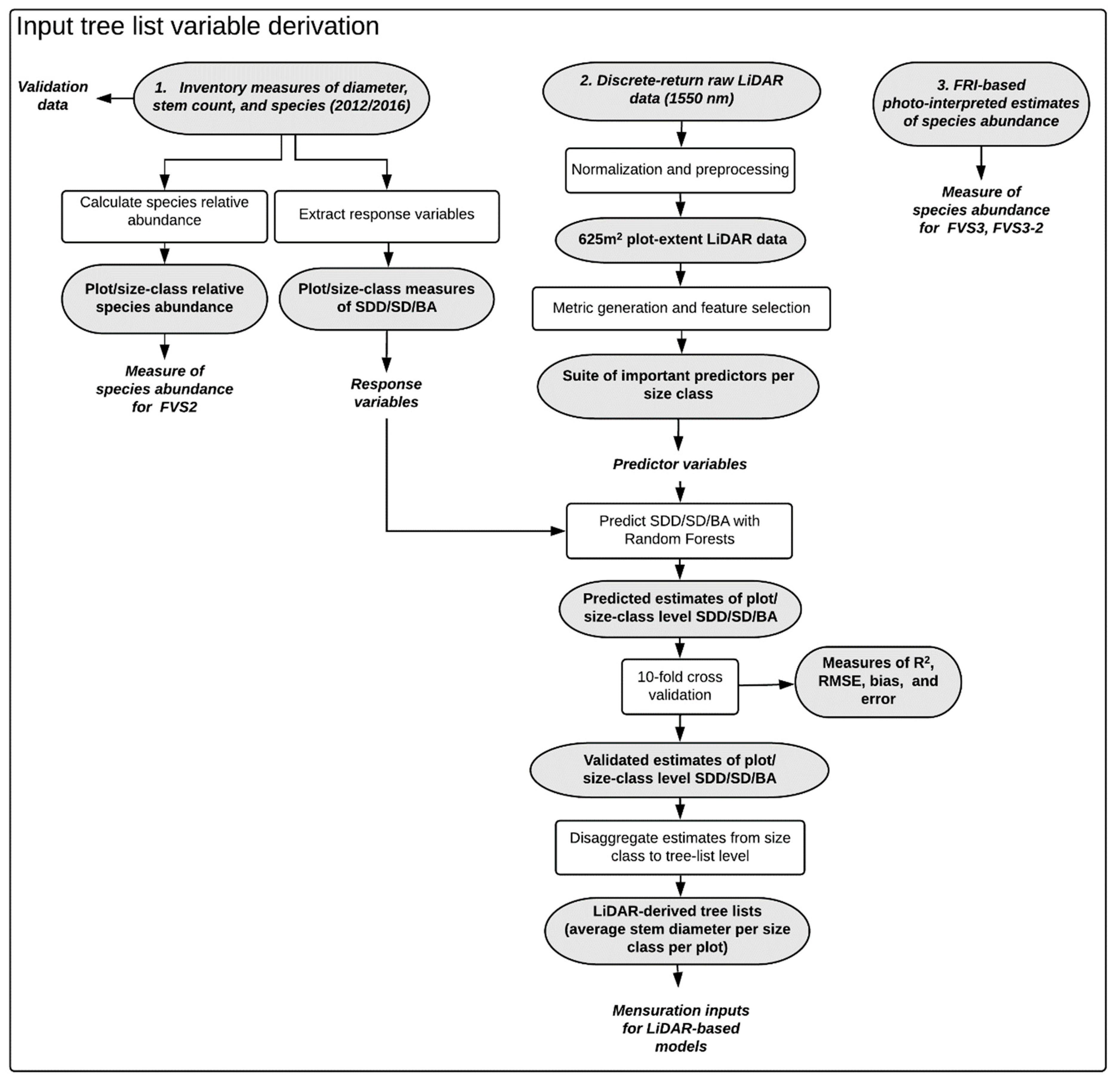
3.1. Deriving Tree Lists

Differences between RMSE and RMSEcv were small, indicating the SDD, SD, and BA_dist models were stable (
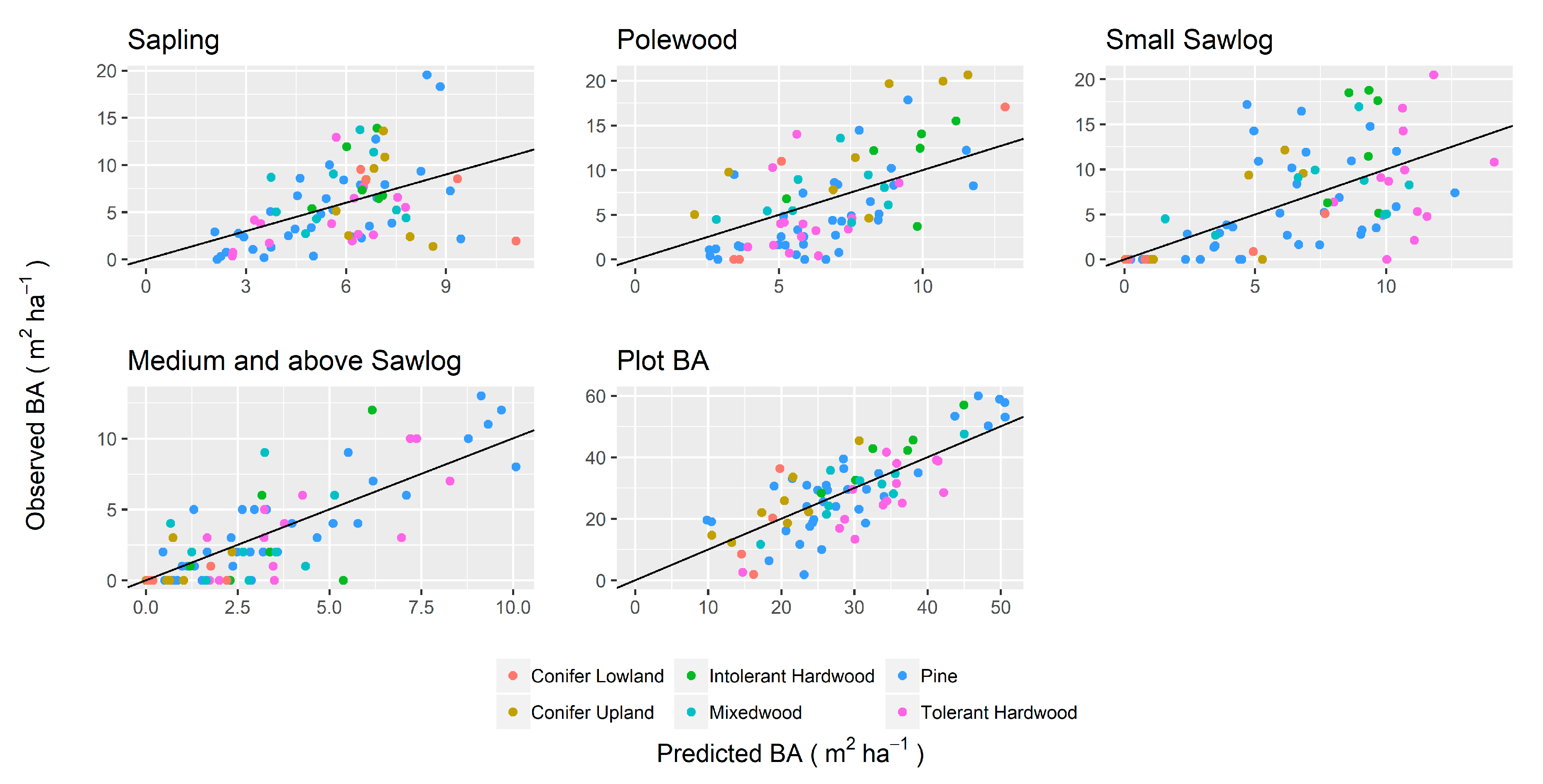
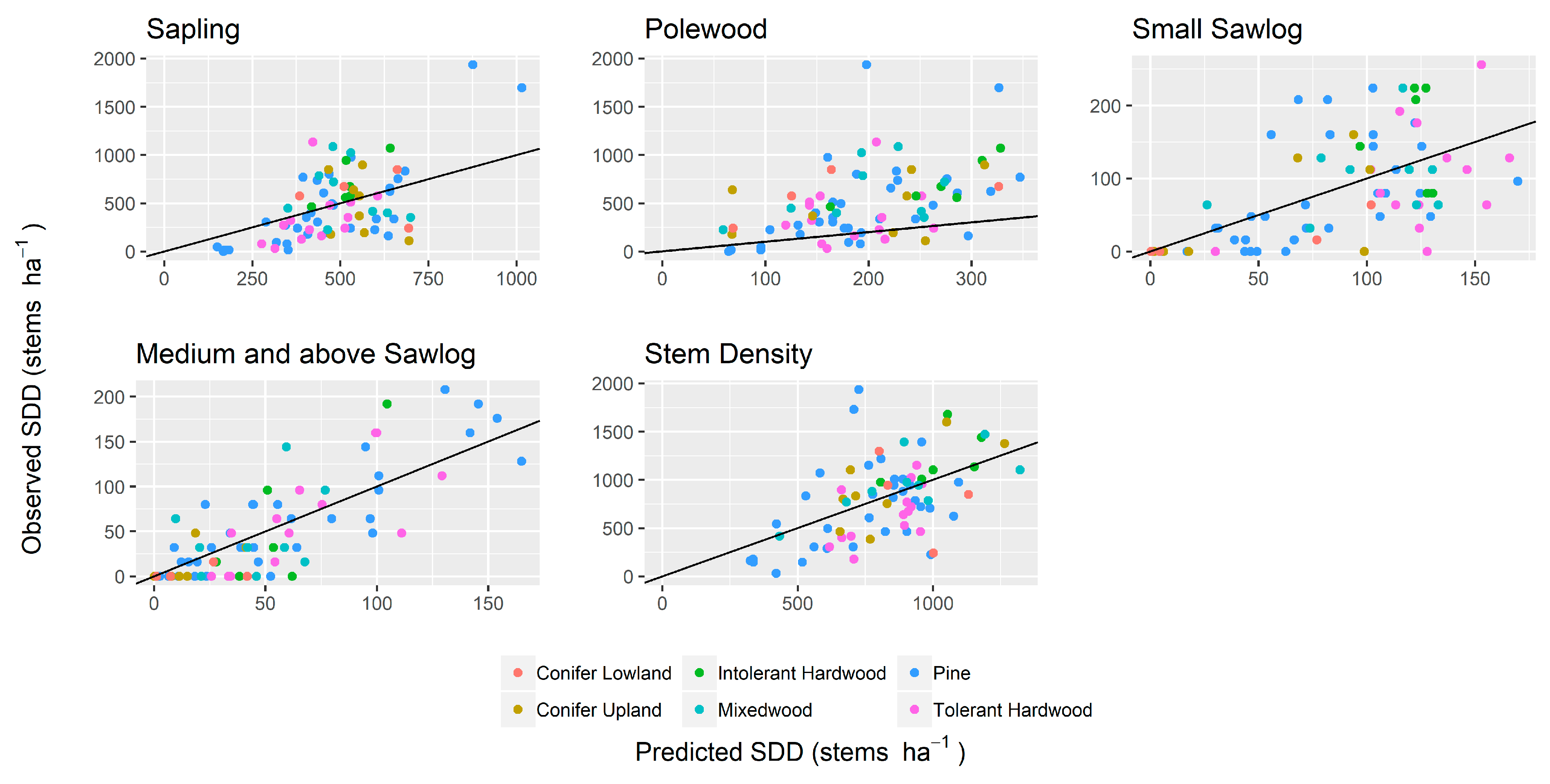
Table 4). BA_dist was predicted with moderate accuracy, with plot-level predictions and medium and above sawlogs having the highest predictive accuracy in the model validation. rRMSE was lower for BA_dist than SDD/SD, indicating that BA_dist was better predicted relative to the mean value. However, both predictions had higher sRMSD (i.e., higher standard deviations of errors). In general, BEI was high, i.e., 0.84, 0.67, 0.34, 0.75, 0.76, and 0.64, for PIN, THW, INT, CU, CL, and MX, respectively (0.73 averaged over the four size classes). Observed and predicted values of BA_dist and SD/SDD by forest type are presented in Figure 5 and Figure 6 respectively.
We omitted the FVS3-2 model from the further discussion due to poor results. To investigate LiDAR-projected carbon accumulation values compared to FVS1 projections, additional comparisons were made to FVS1 for both carbon stocks and accumulation at the plot and size-class level to investigate any statistical equivalence; none of the models showed a statistical equivalence of proportionality (p > 0.05) for either mortality rate, although some had equivalent means. Additional comparisons were made for carbon accumulation. Interestingly, while we did find that the means yielded equivalent results at both mortality rates, proportionality remained underpredicted by the LiDAR-based models.

3.2. G&Y Modelling for Carbon Stocks at Model Initialization and Four-Year Projection

When compared to initial (2012) validation carbon stocks (i.e., FVS1 initialization), we found low correlation across all plot-level models and generally high deviations from the mean and spread of variation (
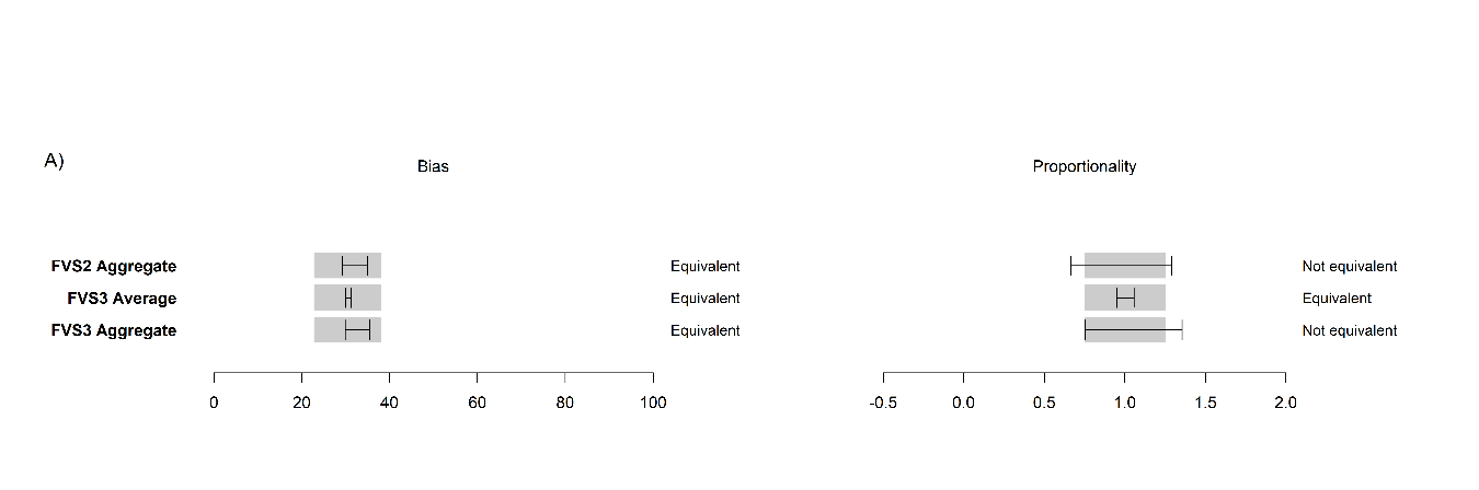
Table 5). The plot-level model with the highest correlation was FVS3 aggregate (R = 0.16), slightly higher than the FVS2 aggregate equivalent (R = 0.12); this stayed relatively consistent when projected to 2016. LiDAR-initialized models generally had a low bias, while aggregate and average models had similar bias across inventory versus FRI species models.
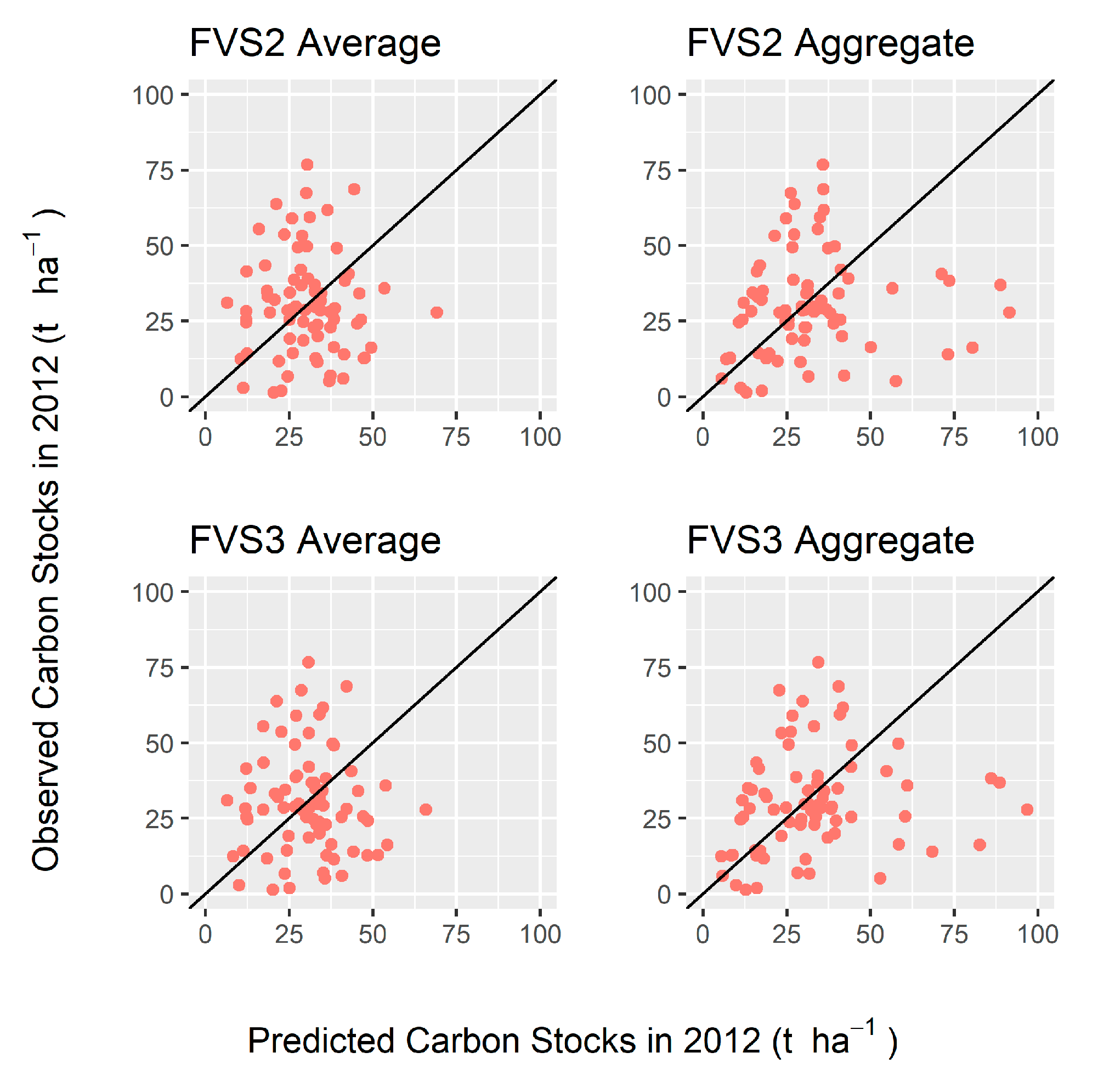
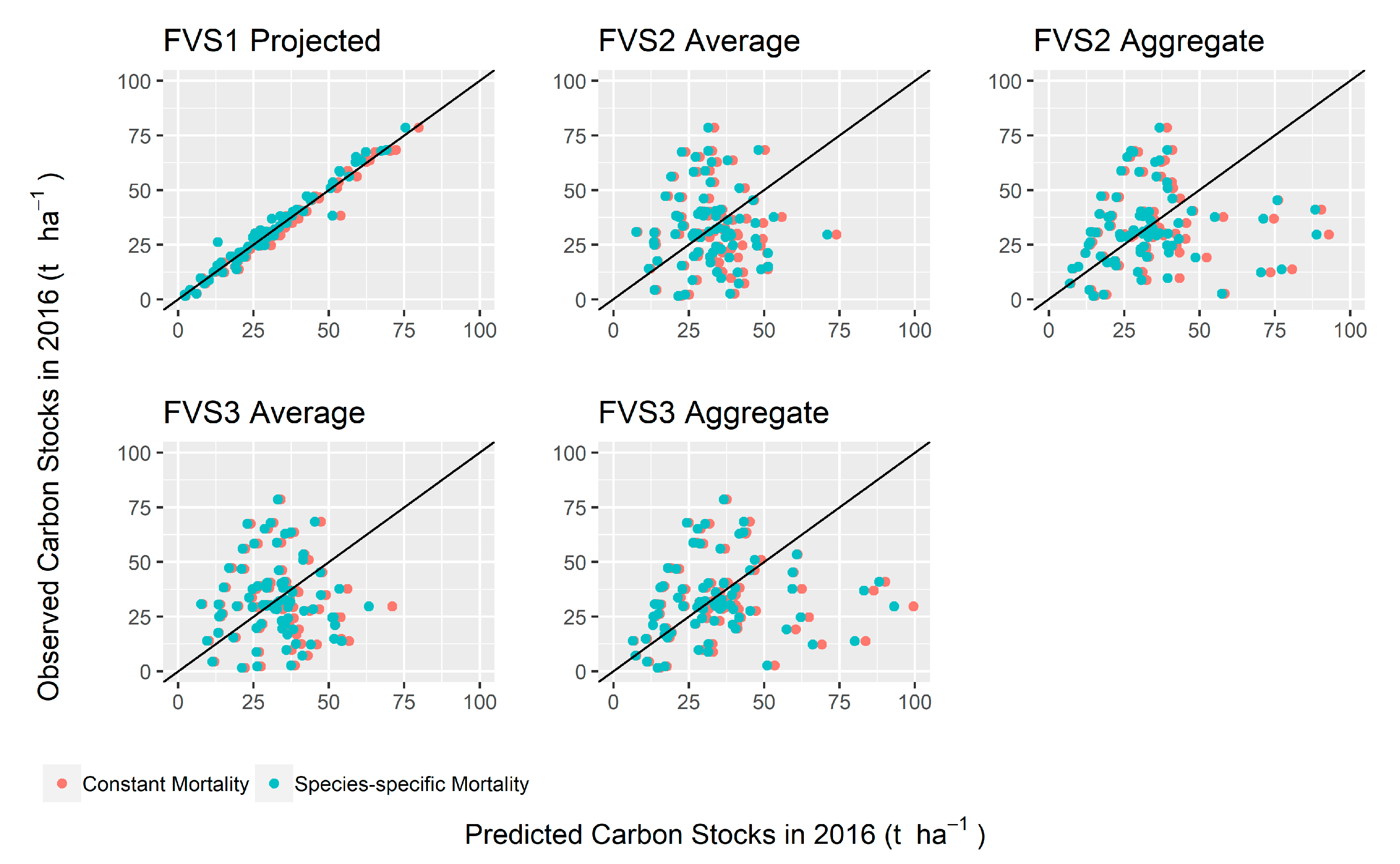
The equivalent FVS average models were not correlated for 2012 or 2016. None of the models were proportionally equivalent to inventory carbon stocks but were statistically unbiased. FVS2 and FVS3 aggregate models had high heteroscedasticity in observed versus predicted values (Figure 7), becoming increasingly variable at higher carbon stocks; this did not stabilize in 2016 (
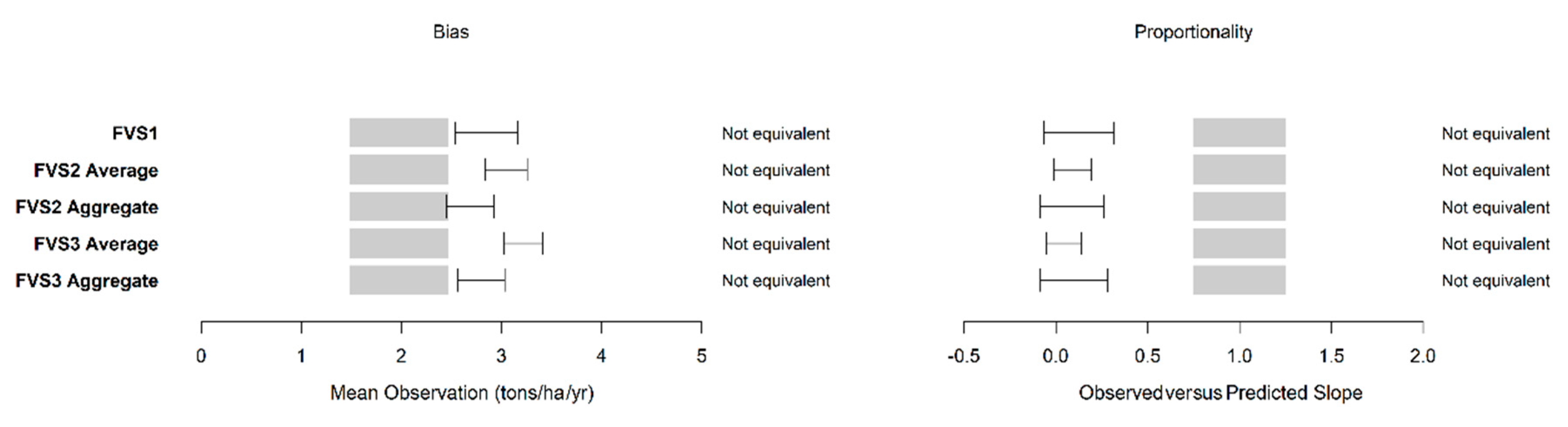
Figure 8). FVS1-projected was statistically equivalent to inventory measures of carbon stocks for 2016 for bias and proportionality at both constant and species-specific mortality rates (R = 0.99, 0.98, respectively). There was no statistical difference between projected values of carbon stock in 2016 for either mortality scenarios for LiDAR-initialized models, referring to the range of CIs within proportionality.
At a size-class level, projections varied widely across both years (Table 6). None of the LiDAR-initialized size-class models were proportionally equivalent to the inventory carbon stocks for either year and were generally highly skewed from the mean and had a high spread of variance; models remained stable in 2016. Mortality rates had negligible effects on the overall model accuracy and bias.
FVS1 was equivalent in both bias and proportionality to 2016 inventory carbon stocks, except for the polewood size class at constant mortality where proportionality was closer to the 0.0−0.3 range (i.e., consistently underpredicting) where a value of 0.75 is the minimum CI range considered equivalent. FVS1 saplings at both mortality rates were proportionally equivalent but not equivalent in bias.
On a forest-type level, there were some variances in correlation in 2012, especially for the CU group (n = 8; R = 0.70 for FVS2 Aggregate; R = 0.76 for FVS3 aggregate). Generally, groups were consistent with overall results, with a high spread of variation that ranged from rRMSE = 0.39 for FVS3 aggregate in the INT group (n = 6), to 2.42 in the FVS2 aggregate CL group (n = 9). For 2016, these correlations remained relatively consistent (CU FV2 aggregate R = 0.73 at constant mortality; FVS3 aggregate R = 0.79 at both mortality rates). For size classes, forest types still had high deviations from observed values at both years. Carbon stocks for CU medium and above sawlogs had a moderate correlation with inventory data for both inventory and photo-interpreted (FRI) species models in 2012 (R = 0.42, 0.43, respectively), however, these values were extremely far from the observed mean and had a high spread of variance (rRMSEmax = 12.91; sRMSDmax = 6.77). THW small sawlogs had similar correlations (i.e., R = 0.37 and 0.34, for FVS2 and FVS3, respectively), with lower deviations from the mean and lower spread of variance (rRMSEmax = 0.83; sRMSD%max = 1.01). INT saplings had a higher correlation for FVS3 at R = 0.57, and had a similar trend in mean and spread of variation, at rRMSE = 0.94 and sRMSD = 2.88.

3.3. G&Y Modelling of Carbon Accumulation (2012 to 2016)

Carbon accumulation predictions were highly biased and had high rRMSEs and sRMSDs (
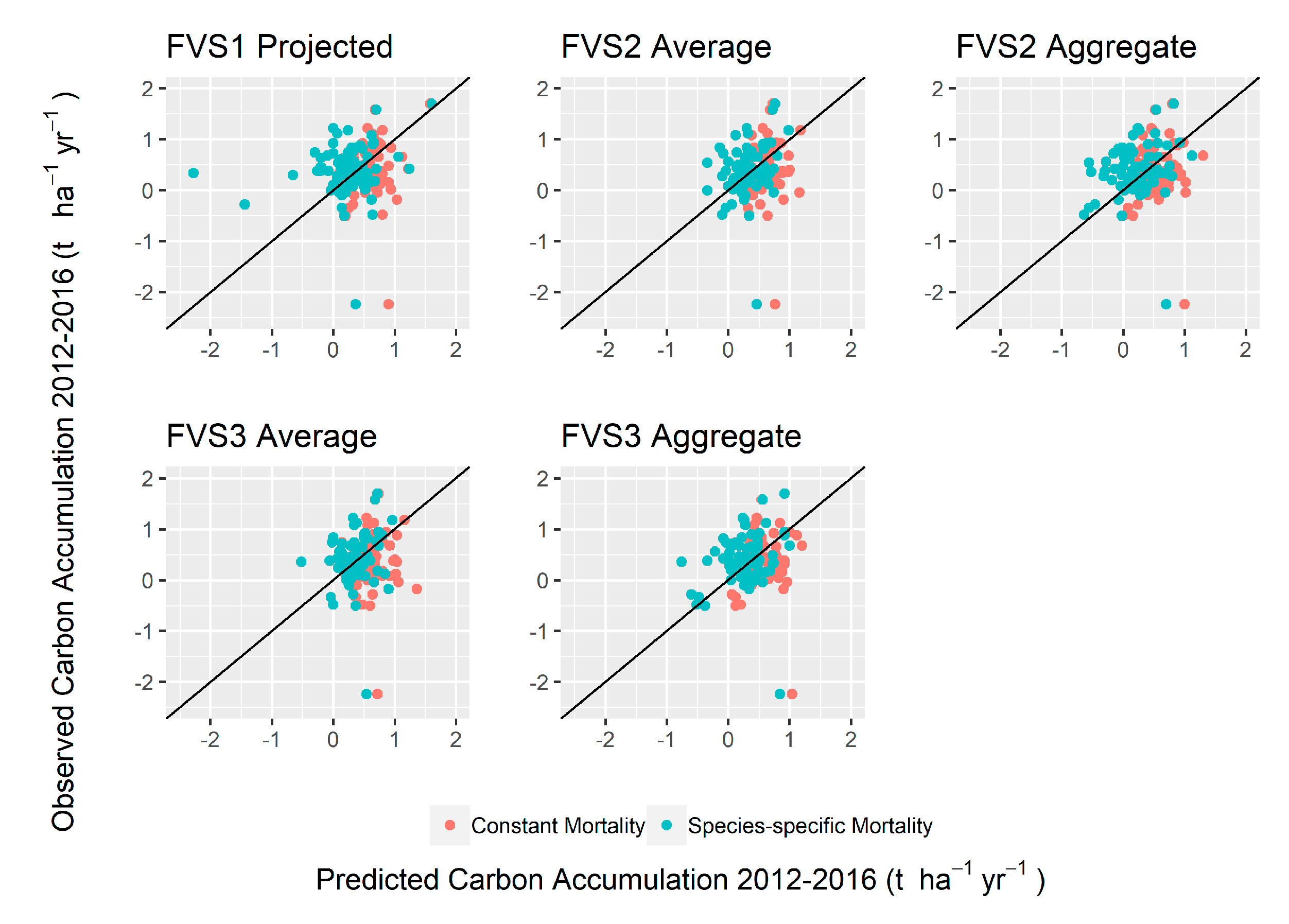
Table 7). In contrast to carbon stock projections, carbon accumulation was not statistically equivalent for the baseline FVS1-projected model for either bias or proportionality to measured inventory-based accumulation at either mortality rate, where a constant mortality rate generally overpredicted, and a species-specific mortality rate underpredicted mean accumulation (Figure 9).
Correlation between LiDAR-initialized model values and inventory rates were comparable to 2012/2016 carbon stock projections (e.g., 2012 FVS2 aggregate R = 0.16; 2016 R = 0.11; accumulation constant mortality R = 0.13, species-specific mortality = 0.17), with comparable spreads of variation (i.e., sRMSD), however, predictions were considerably higher than the observed means (i.e., higher rRMSE). Compared to predictions of carbon stock, accumulation predictions were either largely systematically over or under-predicted. Accumulation appeared consistent across both FVS1 and LiDAR-initialized models, with the exception of a few outliers for FVS1 (Figure 10).
At the size-class level, none of the models were proportionally equivalent to inventory-based accumulation, although some models were statistically equivalent to the mean (i.e., the models were equivalent in bias). RMSE was still high for all groups, although some models had high correlations and similar distributions of values visually.
On a forest type level, some incremental improvements in correlation and error were observed, while some models were several orders of magnitude under- or over-predicted versus the mean observation. Specifically, the accumulation from INTconstant, CLconstant, and CLspecies-specific forest types all had rRMSEs greater than ±5.00. The strongest predictions were for the PIN type, with the FVS1 mean approaching an rRMSE of 0.78 for constant mortality and 1.01 for species-specific mortality, comparable to 0.78 for the FVS3 aggregate constant mortality model, and 0.88 for the species-specific model; bias was generally positive for constant mortality (FVS1 bias = 15.5%) and negative for species-specific mortality (FVS1 bias = −41.13%).

3.4. Influence of Species Designation on Carbon Stock Predictions

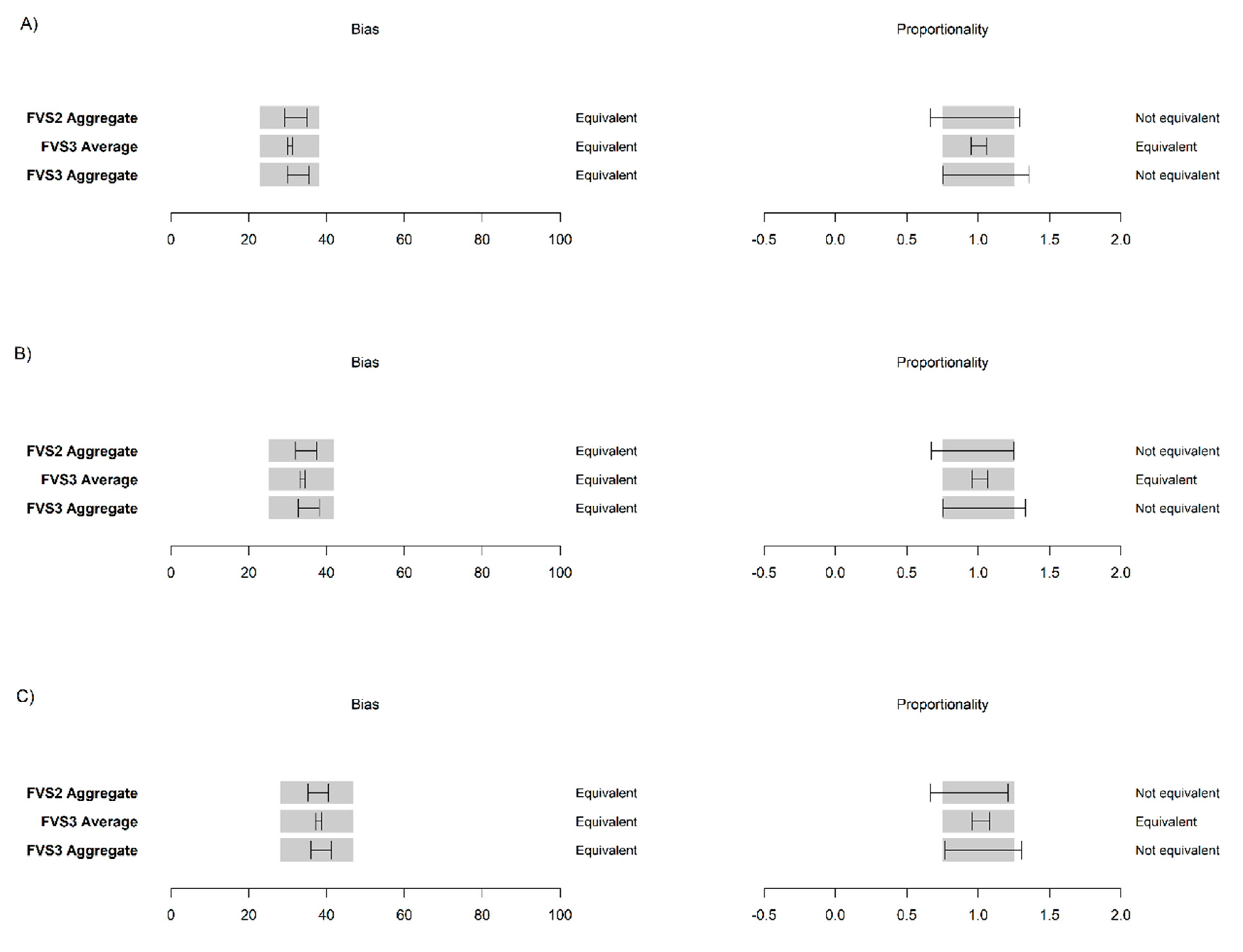
At the plot-level, FVS2 was statistically equivalent to FVS3 for 2012, 2016, and a nine-year projection at both mortality rates, shown here for FVS2 average at constant mortality (Figure 11, S4).
At the size-class level, predictions were more varied. Medium and above sawlogs were not equivalent in proportionality (p > 0.05) for 2012, 2016, or 2021, however, they were equivalent in bias for both years. In contrast, small sawlogs and polewoods were found to be equivalent in bias and proportionality in all three years at both mortality rates for FVS2 to FVS3 equivalent models. Testing constant mortality, carbon stock projections grouped by forest types held equivalency for 2016 except for the INT and MX types. We did not test by size class due to the insufficient number of plots needed to perform a meaningful statistical equivalence test.

3.5. Influence of Species Designation on Carbon Accumulation Predictions

Carbon accumulation was generally not equivalent when compared between LiDAR-initialized models at the plot level. FVS2 aggregate models were equivalent to FVS3 aggregate models at the constant mortality level for 2016 and 2021, but not for species-specific mortality. Similar trends were observed at the size class level. Medium and above size class accumulation rates were equivalent for 2016 and 2021 for constant mortality, but were not equivalent for species-specific mortality, while saplings were not equivalent at either rate at either year. Small sawlogs and polewoods were equivalent at both years in both bias and proportionality for constant mortality, but not for species-specific mortality. Accumulation by forest type (i.e., PIN, THW, INT, CU/CL, MX) did not retain proportional equivalency for constant mortality for 2016 and thus was not examined for 2021.

4. Discussion

To the best of the authors’ knowledge, no study has projected carbon accumulation in mixed temperate stands using local G&Y models from LiDAR-initialized tree lists and photo-interpreted species abundance data. We determined the utility of LiDAR-initialized G&Y models to improve estimates of carbon accumulation and carbon stocks in an understudied mixedwood temperate forest compared to projections using inventory data. We also sought to understand the importance of precise species abundance data on predictions of carbon accumulation and carbon stock using a locally-tailored model.
Equivalence testing indicated that neither FVS2- nor FVS3-based carbon accumulation or carbon stocks at any size class and at the plot level were equivalent to inventory-initialized estimates at a four and nine-year projection, emphasizing the difficulty in parameterizing models for complex temperate forests with moderate-to-poor SDD/SD and BA_dist predictions. Inventory-based FVS1 predictions were equivalent for carbon stocks, but failed to maintain equivalency for 2012−2016 accumulation compared with validation data, signifying that accumulation is more sensitive to precise parameterization than carbon stocks. A key finding was that FVS2 and FVS3 (i.e., inventory-based measures of species abundance and photo-interpreted species, respectively) were equivalent for most size classes and at the plot level (p < 0.05). They were also generally equivalent when examined at a forest type level for carbon stocks, but not for accumulation. This finding suggests that predictions of species abundance from LiDAR (e.g., [5,81]) may possibly be replaced in studies where photo-interpreted estimates are available for the purpose of improving carbon stock estimates and broad accumulation estimates. Testing mortality rates showed that the constant mortality rate was more effective due to the high variability that species-specific rates caused, especially for photo-interpreted parameterization. Furthermore, these data are spatially-explicit and can be used in conjunction with LiDAR data to initialize tree-lists and map carbon accumulation at the forest level.

4.1. Assessment of BA_dist, SDD, and SD Attribute Predictions

Model predictions of BA_dist were better than SDD and SD predictions. Results were favourable in comparison to other studies that predicted BA_dist from LiDAR in similar forest types; i.e., Spriggs et al. (2017) [18] reported an rRMSE of 22% and 33% in sugar maple and mixedwood plots, respectively (plot size = 2500 m2), Vauhkonen & Mehtätalo (2014) [82] reported an rRMSE of 13–68% (Scots Pine plantations; plot size = 400 m2), Lamb et al. (2017) [83] reported an rRMSE of 36.6% in spruce plantations; compared to 29% in this study.
Falkowski et al. (2010) [5] used a k-NN/RF imputation approach to predict SDD/SD and BA_dist in a conifer-dominated forest, achieving a correlation of 0.88, considerably higher than our findings (R = 0.62), while their best-performing SD model performing similarly to ours (R = 0.29; R = 0.28, respectively). Our small trees had lower correlations compared to their best sapling model (R = 0.49, compared to R = 0.32 in this study) although our definition of sapling was more constrained (i.e., 8–17 cm DBH, versus 8–18 cm). Although not evaluated in this study, they also reported that none of the measured forest inventory variables, including total BA_dist and SD, were proportionally equivalent to validation data at the ±20% equivalence level (p < 0.05). Spriggs et al. (2017) [18] discussed the difficulty in predicting smaller stems, particularly in closed canopies where understory returns are limited. Hudak et al. (2008) [25] reported a high correlation (R = 0.80) for BA_dist in a similar mixed conifer forest, comparable to the results reported here (R = 0.79). Using an ITC approach, Lindberg et al. (2010) [84] achieved rRMSEs of 37% for SD in a mixedwood forest, close to the 43% reported here, while Vauhkonen and Mehtätalo (2014) [82] reported an rRMSE of 27.6% for SD.
RF is a common non-parametric algorithm used in forestry attribute prediction [75]. The challenge encountered in this study was the difficulty in accurately predicting SDD and BA_dist values when there was an absence of trees for a given size class. This was most pronounced for medium and above trees across all forest types resulting in an over-prediction of carbon stock values for a considerable proportion of plots. Here, we saw a consistent bias in our observed and predicted values, where a considerable number of plots had no medium or above diameter trees, but the RF model for BA_dist and SDD predicted the presence of trees. This could be due to the inherent characteristic of RF to average predicted values, where a prediction of zero is unlikely in RF regression trees. Shang et al. (2016) [85] suggested that in attribute prediction, larger size classes could be pooled together to improve model performance of SDD predictions. Following this directive, sRMSD for medium and above size classes was 59%, considerably lower than the sRMSD reported for their 38–50, 50–62, and 62 and above size classes (sRMSD = 78, 80, and 89%, respectively). However, we found that following this protocol ultimately did not translate to statistically equivalent measures of carbon stock or accumulation to inventory data.
The SDD model selected intensity metrics for smaller size classes, and height-based metrics for larger size classes. In similar studies where intensity metrics have been used, they have also been selected as important for smaller size classes [14]. Although intensity helped in predicting these small size classes (as measured by %IncMSE), it ultimately did not lead to proportional equivalency for carbon stocks or accumulation. Conversely for BA_dist, only height variables were selected and still resulted in a considerable decrease in G&Y model accuracy (i.e., FVS3-2).

4.2. Assessment of G&Y Models

Again, to our knowledge no studies have forecasted carbon accumulation using a predicted average-DBH tree list from LiDAR. Some studies have compared remeasurement data from repeat LiDAR surveys to derive carbon accumulation; Hudak et al. (2012) [76] used repeat LiDAR surveys to quantify carbon accumulation over a six-year period by subtracting LiDAR-predicted biomass, and Økseter et al. (2015) [86] used similar techniques for an 11-year period. In general, our LiDAR-initialized models projecting carbon stock were not equivalent to the inventory stocks in proportionality, regardless of the type of plot-level tree list initialization (i.e., using plot-level SD and BA_dist, or using an aggregated list from size-class level predictions) or whether looking at the size-class level. However, aggregate models had a consistently higher spread of values and a consistent underprediction of larger carbon stock plots than average models. Accumulation was more sensitive; our LiDAR-initialized models consistently over- or under-reporting accumulation rates, indicating mortality was not ideally parameterized and should be more carefully considered. Perhaps the addition of an ‘average’ rate could have improved the mean accumulation results. Since results were similar regardless of species abundance data used and regardless of mortality, it implies that further refinement is needed in creating accurate DBH for G&Y model initialization and that perhaps using a distribution of DBH values may improve modeling results. Indeed, perhaps more information is needed that goes beyond the ability of LiDAR to provide for carbon stocks or accumulation, and that integration of more ancillary data is necessary, such as aerial photography, Sentinel-2 A or other remotely-sensed data to provide stronger initial estimates of BA_dist and SD/SDD prior to G&Y modeling [87,88].
Our findings indicate an agreement of carbon stock values for FVS1 at the plot and size-class level with validation data (except for saplings). However, none of the FVS1-projected accumulation models were equivalent to inventory measures. Similarly, Hudak et al. (2012) [76] reported more variability in accumulation when extracted from biomass predictions. Accumulation appeared to be in agreement when looking at observed versus predicted values between FVS1 and LiDAR-based models, with similar rRMSEs (e.g., rRMSEPIN = 77.8% for FVS1; 86.50% for FVS2 aggregate at constant mortality), suggesting that some mechanistic growth patterns were consistent (Figure 6). Because our subsequent equivalence testing indicated the models were still dissimilar proportionally, we stratified the plot-level accumulation models by forest type to identify any consistencies with FVS1 projections, however, this further reduced the accuracy of accumulation results from LiDAR models and means became statistically dissimilar, in addition to the already statistically dissimilar proportionalities. Looking at the highest deviations in plot-level accumulation across model types (Figure 6), we examined five plots that were clear visual outliers, two of which were consistent across model types. For constant mortality, plot number 026, an intolerant hardwood type consisting mainly of B. papyrifera, P. grandidentata, A. rubrum, and A. saccharum had a predicted accumulation rate of 0.9 Mg/ha/yr, compared to an actual rate of 2.24 Mg/ha/yr. For FVS1, these extreme deviations typically occurred at species-specific mortality rates and within CU and INT groups (e.g., plot number 075 predicted 0.34 Mg/ha/yr versus −2.28 Mg/ha/yr CU; plot number 026 −0.36 Mg/ha/yr versus −2.24 Mg/ha/yr INT). Studies have previously identified conifers as being difficult to capture with LiDAR due to the reflective properties of crowns, however, these inaccuracies were also present in the inventory model [18]. Given that these outliers were generally more pronounced with species-specific mortality rates, it is likely that our models did not parameterize ideal rates for specific hardwoods and that future consideration of mortality rate should be more carefully reviewed.
We did not expect to see statistical equivalencies for carbon stock and accumulation forecasts for FVS2 and FVS3 (meanFVS2STOCK2016_CONST = 33.48 tons/ha, meanFVS3STOCK2016 = 33.74 tons/ha, meanFVS2ACCUMULATION_CONST = 3.22 tons/ha/yr, meanFVS3ACCUMULATION_CONST = 3.22 tons/ha/yr).The majority of photo-interpreted species data was from 2009, with a smaller proportion from 2014. This two-to-three-year age gap between LiDAR and species abundance data collection suggests that the species composition played less of a role in initializing the G&Y models compared to DBH, even for a G&Y model that includes species-specific allometric equations. This emphasizes the need for a renewed call on accurate inputs of DBH as the primary driving factor of a more accurate carbon accumulation forecast. We also expected less of an agreement as the model was projected into 2021, however, the LiDAR-based models still retained statistical equivalency for specific combinations; i.e., accumulation models retained equivalency for the aggregate model with constant mortality over the nine-year scenario, suggesting that better predictions of larger size classes influenced the consistency of carbon accumulation predictions. We did find some discrepancies between LiDAR-based models for certain size classes. Because saplings grow at a faster rate, we did not expect photo-interpreted species to be proportionally equivalent as growth occurs at a faster rate for young trees, thus precise parameterization of species would have more influence here. There was a closer agreement between FVS2 and FVS3 at species-specific mortality for medium and above carbon stocks; however, this size class only retained accumulation equivalency at a constant mortality rate. Because a species-specific mortality rate coupled with an imprecise species characterization could further skew values, the use of the constant mortality rate is preferred. Ultimately, future work could also compare the results of forest attribute modeling with LiDAR-derived species abundance and photo-interpreted estimates for potential model improvement.
As species abundance is data and resource-intensive to calibrate due to the high range of forest conditions needed to be captured [89], it may be prohibitive to initialize models based on remotely-sensed predictions. Previous studies at PRF have attained varying levels of success in species abundance modelling (e.g., classification accuracies of 64% P. strobus, 53.7% Q. rubra, 79% P. resinosa, 49% B. papyrifera, 79.9% A. saccharum, 33.5% A. rubrum, 51% P. glauca, Gougeon and Leckie, 2011 [90], using an ITC approach; R = 0.69, 0.74, 0.85, 0.53, 0.73 for P. strobus, P. resinosa, P. glauca, P. betula/populus, Acer spp., van Ewijk et al., 2014 [81], using boosted regression trees [BRTs]). Falkowski et al. (2010) [5] found that predicting species abundance did not produce statistically equivalent results to inventory measurements (p < 0.05), however, projections of BA_dist initialized using FVS still followed similar trends to inventory-initialized projections. Thus, using photo-interpreted species abundance may be preferred in complex forests where individual-tree species information is required for G&Y model initialization and for which these data are available. Falkowski et al. (2010) [5] also demonstrated that it may be possible to achieve statistically equivalent results of growth when using non-inventory-equivalent predicted species abundance with BA_dist projections, rather than estimating tree lists and explicitly projecting carbon stock values. This also suggests that the allometric equations we used in converting diameter to carbon stock may introduce large amounts of error, thereby requiring further refinement.
The removal of the less accurate SDD in predictions and using only BA_dist (i.e., FVS3-2) resulted in statistically different models on average that were less effective than the combined SDD/BA_dist plots, implying that regardless of the low SDD accuracy, it remained a key component in obtaining more accurate tree lists. However, other attributes, such as quadratic mean diameter (QMD) could also be used instead of SDD to further improve predictions, given that QMD has shown improved predictions compared to SDD (e.g., [9]). Another alternative could be using a predicted distribution of values, capturing a higher range of diameters than the mean (i.e., PDFs; Olofsson et al., 2008 [91]). Unpublished work by van Ewijk (2015) [92] used height-diameter relationships to estimate diameters from LiDAR-derived height distributions, albeit discovering that this characterization was not sufficient for generating accurate tree lists for FVSOntario initialization.
Given that we had plots with negative accumulation for some years in the validation data, we additionally tested whether the removal of negative mortality would improve model estimates for both inventory and LiDAR-based models using a constant mortality rate. We found that this did not make a large impact on predicted values and that both the inventory and LiDAR-based models were still not equivalent to the validation data for 2016. This suggested that there were additional underlying mechanisms not captured by the G&Y model.

4.3. Limitations and Future Work

Various considerations in this study may have contributed to errors that propagated throughout the modelling effort. One limitation relates to plot size, which was relatively small (i.e., 625 m2); for instance, Shang et al. (2016) [85] achieved a BEI of 0.49 for 400 m2 plots versus a BEI of 0.39 for 1000 m2 plots. Given our BEI of 0.73, increasing plot size may have decreased our attribute prediction error so long as plot number is not reduced [93]. It is well-established that a larger plot would reduce the ‘edge effect’, or the difference between field-based plot and LIDAR-based characterization of trees in the same radius (i.e., nature of the canopy captured in the point cloud). For instance, a tree right outside the plot boundary but leaning in towards the plot would be excluded from any mention in inventory data; however, the canopy itself would still be captured in the equivalent LiDAR return, thereby influencing LiDAR metrics and the prediction of variables [11,84]. Because forests are complex and the full range of forest dynamics is not yet understood, a modelling approach incorporating a stochastic element could have generated more amenable results [94]. In addition, a larger number of plots would have enabled us to examine more relationships between model parameterizations and predictive success, for instance further comparing carbon stock and accumulation by forest types at each size-class level.
As with any modelling exercise, a variety of conditions and sensitivities may or may not be captured to characterize the full range of effects. Our data were stratified by common forest types of Ontario based on species abundance ranges in our data; however, stratification by NDVI, forest structural groups, aspect, slope, elevation, etc., may have enhanced model performance [75].
While we tested for mortality across all modelling approaches, our value for species-specific mortality rate was chosen somewhat arbitrarily based on the differences between 2012 and 2016 live trees. Because FVSOntario had a limit of maximum stand stocking density [95], using the model-supplied internal mortality logic would often result in a massive die-off of trees due to our sometimes-high predictions of stems, thus we were constrained to a user-defined rate. As our defined mortalities often resulted in either under- or over-predictions of LiDAR-based carbon stock and accumulation, it is recognized as an important parameter. Future work should strive to improve the methodology for selecting the most appropriate mortality rate for G&Y models especially when used with LiDAR-initialized tree lists.
At the same time, other studies examine plantations consisting of commercial tree species, rather than a range of dynamic conditions such as in PRF. Boisvenue et al. (2019) [96] highlight this problem, noting that often, commercial tree species are heavily favoured in sampling, and the use of allometric equations from a limited number of samples often leads to increased error, compounded with the fact that the allometric equation itself may affect estimation of carbon stocks/accumulation. PRF contains a multitude of stem sizes and classes, the smallest of which (<8 cm) were not included in this study, partially due to the assumption that the relative total BA_dist of these trees makes them negligible in carbon accumulation, if not for the fact that their height and relative width make them difficult for LiDAR to capture. We set a height threshold of 1.37 m for this study, below which returns were assumed to be ground returns and ignored in metric calculation. However, smaller (i.e., younger) trees grow faster than large (i.e., older) trees and thus accumulate carbon at a faster rate [88]. The exclusion of these trees in our inventory and in subsequent modelling could be a missing component that contributes to predicted carbon accumulation (i.e., under-estimating carbon accumulation). However, capturing the true proportion of BA_dist and SD/SDD contained within this size class remains challenging given the lack of resources to collect during field campaigns. If a sampled plot contains only one large tree and an abundance of <8 cm DBH trees, it is plausible that these trees accumulate a total amount of carbon large enough for carbon accounting and reporting. There may be a relationship between the proportion of BA_dist in <8 cm trees and canopy metrics that can be explored in a future study to capture the fullest extent possible of the aboveground live carbon domain. Similar work has been reported by Maltamo et al. (2004) [39], using tree height distribution as a proxy for estimation of smaller stems, finding poor accuracy for these suppressed trees.
Although beyond the extent of this modelling exercise, Penner et al. (2015) [31] and Breidenbach et al. (2008) [97] suggested that there are possible improvements in SDD predictions at larger stand or forest levels; extrapolating the FVSOntario model over a larger area may improve predictions of carbon accumulation in a future study, albeit noting the model would need to be modified to allow for spatially-explicit modelling. Previous studies with access to spatially parameterized G&Y models have done this for SD and BA_dist (e.g., [5,89,98]).
Many studies have successfully implemented LiDAR-derived metrics for forest attribute modeling [25,75,87,99,100]. Recent studies have also used LiDAR for mapping aboveground carbon density [23] or using repeat LiDAR surveys to map biomass and establish accumulation rates based on these differences [76,101]. However, without the access of repeat LiDAR for future projections, accumulation is usually implied from rates of BA_dist growth, which limits our ability to fully report on carbon sequestration and gain a more holistic sense of Canada’s potential for sequestration in understudied complex temperate forests. Looking ahead to the future of LiDAR and carbon management, the new successfully launched Global Ecosystem Dynamics Investigation (GEDI) is gaining considerable attention [102]. Given this study’s finding that photo-interpreted estimates from various years can provide equivalent estimates to inventory-level data, future studies should also look to investigate the application of space-based LiDAR and coincident species abundance data for areas with less access to ground data to improve estimates of carbon accumulation.

5. Conclusions

Lidar has been shown to be a valuable and reliable tool in forestry for spatially-explicit modeling of forest stand attributes (e.g., [9,10,16,18,25]). In the context of G&Y modelling, LiDAR-derived tree lists for initializing G&Y models of direct carbon stock and accumulation have not been tested, which could lead to new insights for climate change mitigation in forest management practices. Complex temperate forests remain understudied in G&Y research; improving G&Y techniques in this area could benefit climate change mitigation and sustainable forest management. This study examined methods for improving estimates of carbon accumulation and carbon stock using a LiDAR-derived G&Y model in an uneven-aged, mixedwood forest of Ontario, Canada. Our predictions of forest variables using the non-parametric RF algorithm were found to be comparable to other studies, however, small-diameter trees, particularly saplings and polewoods, were less well predicted by LiDAR. We demonstrated that predicting carbon stocks across a range of size classes and forest types were more accurate than predicting carbon accumulation, but neither model output achieved statistical equivalence across a range of forest types compared to inventory data. Thus, the information demands for accurate G&Y modeling of carbon accumulation in complex stands remain beyond the reach of current LiDAR and nonparametric modeling approaches. However, our findings suggest this gap is also due to high parameterization costs of the G&Y model, such as mortality, and that these remain areas of focus.
Statistical equivalence was achieved between LiDAR-based models, suggesting complex forests could benefit from photo-interpreted estimates to achieve the same results as inventory-derived species abundance, possibly bypassing the need for predicting species information in carbon accumulation studies. However, this area requires further study, including why these consistencies do not hold across forest types. Models tended to perform better using constant mortality rates when initialized with photo-interpreted species, which could be explained by the need to balance imprecise species with a more generalized mortality rate. The potential of using photo-interpreted species abundance estimates for areas where such data exists as a potential replacement or comparison for LiDAR-derived species abundance is a novel contribution in this study.
This study explored the various considerations for establishing a G&Y model in the understudied uneven-aged mixed forests of Ontario. Models are inherently deficient due to the complexity of the systems studied; thus assumptions can be flawed. Additionally, it is important to note that field data may not provide any more “true” estimates than LiDAR models, and come with their own inherent measurement and sampling errors. Future studies should continue to explore what parameters are crucial for improved estimates of complex forest carbon accumulation.

Supplementary Materials

The following are available online at https://0-www-mdpi-com.brum.beds.ac.uk/2072-4292/12/1/201/s1, S1: An explanation of deriving basal area from stem diameter distribution; S2: Explanation of measures of accuracy; S3: A detailed explanation and example of FVS model parameterization, execution, and validation, and S4: Additional tables for model outputs for Figure 11.

Author Contributions

Conceptualization, P.T.M., K.Y.V.E, P.M.T., and N.A.S.; methodology, P.T.M., K.Y.V.E., P.M.T., and N.A.S.; software execution, P.T.M. and D.C.E.R.; validation, P.T.M.; writing—original draft preparation, P.T.M.; writing—review and editing, P.T.M., K.Y.V.E., P.M.T., N.A.S., and D.C.E.R.; supervision, P.M.T. and N.A.S.; funding acquisition, P.M.T. and N.A.S. All authors have read and agreed to the published version of the manuscript.

Funding

This project was funded in part by Queen’s University, the Government of Ontario, and the Natural Sciences and Engineering Research Council (NSERC) Discovery Grant awarded to P.M.T. We are grateful to funding from the NSERC Collaborative Research Development Grant – Assessment of Wood Attributes from Remote Sensing (AWARE) project (P.I. Nicholas Coops) that funded the field data collection in 2016–2017.

Acknowledgments

We are grateful to Advanced Forest Resource Inventory (AFRIT), who provided the LiDAR data for this research. We would also like to thank our Petawawa field team, Karin van Ewijk, Paulina Marczak, Rachel Kuzmich, and Shuhong Lin, and to Alex McVittie for automating the FVSOntario software. Special thanks to Chen Shang for additional analytical support and manuscript comments, and to two anonymous reviewers for their insightful comments.

Conflicts of Interest

The authors declare no conflict of interest. The funders had no role in the design of the study; in the collection, analyses, or interpretation of data; in the writing of the manuscript, or in the decision to publish the results.

References

  1. Jandl, R.; Lindner, M.; Vesterdal, L.; Bauwens, B.; Baritz, R.; Hagedorn, F.; Johnson, D.; Minkkinen, K.; Byrne, K.A. How strongly can forest management influence soil carbon sequestration? Geoderma 2007, 137, 253–268. [Google Scholar] [CrossRef]
  2. Le Quéré, C.; Andrew, R.M.; Friedlingstein, P.; Sitch, S.; Pongratz, J.; Manning, A.C.; Korsbakken, J.I.; Peters, G.P.; Canadell, J.G.; Jackson, R.B.; et al. Global Carbon Budget 2017. Earth Syst. Sci. Data 2018, 10, 405–448. [Google Scholar] [CrossRef] [Green Version]
  3. Pan, Y.; Birdsey, R.A.; Fang, J.; Houghton, R.; Kauppi, P.E.; Kurz, W.A.; Phillips, O.; Shvidenko, A.; Lewis, S.; Canadell, J.; et al. A large and persistent carbon sink in the world’s forests. Science 2011, 333, 988–993. [Google Scholar] [CrossRef] [PubMed] [Green Version]
  4. Scott, N.A.; Rodrigues, C.A.; Hughes, H.; Lee, J.T.; Davidson, E.A.; Dail, D.B.; Malerba, P.; Hollinger, D.Y. Changes in carbon storage and net carbon exchange one year after an initial shelterwood harvest at Howland Forest, ME. Environ. Manag. 2004, 33, S9–S22. [Google Scholar] [CrossRef]
  5. Falkowski, M.J.; Hudak, A.T.; Crookston, N.L.; Gessler, P.E.; Uebler, E.H.; Smith, A.M. Landscape-scale parameterization of a tree-level forest growth model: a k-nearest neighbor imputation approach incorporating LiDAR data. Can. J. For. Res. 2010, 40, 184–199. [Google Scholar] [CrossRef]
  6. Vanclay, J. Forest growth and yield modelling. In Encyclopedia of Environmetrics, 1st ed.; El-Shaarawi, A., Piegorsch, W., Eds.; Wiley: New York, NY, USA, 2002; pp. 811–812. [Google Scholar]
  7. Köhl, M. Forest inventory and monitoring. In Encyclopedia of Forest Sciences, 1st ed.; Burley, J., Evans, J., Youngquist, J., Eds.; Elsevier: New York, NY, USA, 2004; pp. 403–409. [Google Scholar]
  8. Brosofske, K.D.; Froese, R.E.; Falkowski, M.J.; Banskota, A. A review of methods for mapping and prediction of inventory attributes for operational forest management. For. Sci. 2014, 60, 733–756. [Google Scholar] [CrossRef]
  9. Tompalski, P.; Coops, N.C.; White, J.C.; Wulder, M.A. Enhancing forest growth and yield predictions with airborne laser scanning data: increasing spatial detail and optimizing yield curve selection through template matching. Forests 2016, 7, 255. [Google Scholar] [CrossRef] [Green Version]
  10. Lim, K.; Treitz, P.; Baldwin, K.; Morrison, I.; Green, J. LiDAR remote sensing of biophysical properties of tolerant northern hardwood forests. Can. J. Remote Sens. 2003, 29, 658–678. [Google Scholar] [CrossRef]
  11. White, J.; Wulder, M.; Varhola, A.; Vastaranta, M.; Coops, N.; Cook, B.; Pitt, D.; Woods, M. A Best Practices Guide for Generating Forest Inventory Attributes from Airborne Laser Scanning Data Using the Area-Based Approach; Internal Report; Natural Resources Canada, Canadian Forest Service, Canadian Wood Fibre Centre: Victoria, BC, Canada, 2013. [Google Scholar]
  12. Wehr, A.; Lohr, U. Airborne laser scanning—An introduction and overview. ISPRS J. Photogramm. Remote Sens. 1999, 54, 68–82. [Google Scholar] [CrossRef]
  13. Hawbaker, T.J.; Gobakken, T.; Lesak, A.; Trømborg, E.; Contrucci, K.; Radeloff, V. Light detection and ranging-based measures of mixed hardwood forest structure. For. Sci. 2010, 56, 313–326. [Google Scholar]
  14. Shang, C.; Treitz, P.; Caspersen, J.; Jones, T. Estimating stem diameter distributions in a management context for a tolerant hardwood forest using ALS height and intensity data. Can. J. Remote Sens. 2017, 43, 79–94. [Google Scholar] [CrossRef]
  15. Gove, J.H.; Patil, G.P. Modeling the basal area-size distribution of forest stands: a compatible approach. For. Sci. 1998, 44, 285–297. [Google Scholar]
  16. Gobakken, T.; Næsset, E. Estimation of diameter and basal area distributions in coniferous forest by means of airborne laser scanner data. Scan. J. For. Res. 2004, 19, 529–542. [Google Scholar] [CrossRef]
  17. Packalén, P.; Maltamo, M. Estimation of species-specific diameter distributions using airborne laser scanning and aerial photographs. Can. J. For. Res. 2008, 38, 1750–1760. [Google Scholar] [CrossRef]
  18. Spriggs, R.A.; Coomes, D.A.; Jones, T.A.; Caspersen, J.P.; Vanderwel, M.C. An alternative approach to using LiDAR remote sensing data to predict stem diameter distributions across a temperate forest landscape. Remote Sen. 2017, 9, 944. [Google Scholar] [CrossRef] [Green Version]
  19. Härkönen, S.; Tokola, T.; Packalén, P.; Korhonen, L.; Mäkelä, A. Predicting forest growth based on airborne light detection and ranging data, climate data, and a simplified process-based model. Can. J. For. Res. 2013, 43, 364–375. [Google Scholar] [CrossRef]
  20. Taguchi, H.; Endo, T.; Yasuoka, Y. Biomass estimation by coupling LiDAR data with forest growth model in conifer plantation. In Proceedings of the 28th Asian Association of Remote Sensing Conference, Kuala Lampur, Malaysia, 12–16 November 2007; Pusat Remote Sensing Negara: Kuala Lumpur, Malaysia, 2007.
  21. Zhang, Q.; Liang, Y.; He, H. Tree-lists estimation for Chinese boreal forests by integrating Weibull diameter distributions with MODIS-based forest attributes from k-NN imputation. Forests 2018, 9, 758. [Google Scholar] [CrossRef] [Green Version]
  22. Cao, Q.V.; Burkhart, H.E. A segmented distribution approach for modeling diameter frequency data. For. Sci. 1984, 30, 129–137. [Google Scholar]
  23. Poudel, K.P.; Cao, Q.V. Evaluation of methods to predict Weibull parameters for characterizing diameter distributions. For. Sci. 2013, 59, 243. [Google Scholar] [CrossRef]
  24. Thomas, V.; Oliver, R.D.; Lim, K.; Woods, M. LiDAR and Weibull modeling of diameter and basal area. Forest. Chron. 2008, 84, 866–875. [Google Scholar] [CrossRef] [Green Version]
  25. Hudak, A.T.; Crookston, N.L.; Evans, J.S.; Hall, D.E.; Falkowski, M.J. Nearest neighbor imputation of species-level, plot-scale forest structure attributes from LiDAR data. Remote Sens. Environ. 2008, 112, 2232–2245. [Google Scholar] [CrossRef] [Green Version]
  26. Maltamo, M.; Kangas, A. Methods based on k-nearest neighbor regression in the prediction of basal area diameter distribution. Can. J. For. Res. 1998, 28, 1107–1115. [Google Scholar] [CrossRef]
  27. Penner, M.; Pitt, D.G.; Woods, M.E. Parametric vs. nonparametric LiDAR models for operational forest inventory in boreal Ontario. Can. J. Remote Sens. 2013, 39, 426–443. [Google Scholar]
  28. Crookston, N.L.; Dixon, G.E. The forest vegetation simulator: A review of its structure, content, and applications. Comp. Electron. Agric. 2005, 49, 60–80. [Google Scholar] [CrossRef]
  29. Tompalski, P.; Coops, N.; Marshall, P.; White, J.; Wulder, M.; Bailey, T. Combining multi-date airborne laser scanning and digital aerial photogrammetric data for forest growth and yield modelling. Remote Sen. 2018, 10, 347. [Google Scholar] [CrossRef] [Green Version]
  30. Vauhkonen, J.; Korpela, I.; Maltamo, M.; Tokola, T. Imputation of single-tree attributes using airborne laser scanning-based height, intensity, and alpha shape metrics. Remote Sens. Environ. 2010, 114, 1263–1276. [Google Scholar] [CrossRef]
  31. Penner, M.; Woods, M.; Pitt, D.G. A comparison of airborne laser scanning and image point cloud derived tree size class distribution models in boreal Ontario. Forests 2015, 6, 4034–4054. [Google Scholar] [CrossRef] [Green Version]
  32. Pitt, D.G.; Woods, M.; Penner, M. A comparison of point clouds derived from stereo imagery and airborne laser scanning for the area-based estimation of forest inventory attributes in boreal Ontario. Can. J. Remote Sens. 2014, 40, 214–232. [Google Scholar] [CrossRef]
  33. Rodriguez-Galiano, V.F.; Ghimire, B.; Rogan, J.; Chica-Olmo, M.; Rigol-Sanchez, J.P. An assessment of the effectiveness of a random forest classifier for land-cover classification. ISPRS J. Photogramm. Remote Sens. 2012, 67, 93–104. [Google Scholar] [CrossRef]
  34. Kukkonen, M.; Maltamo, M.; Korhonen, L.; Packalén, P. Comparison of multispectral airborne laser scanning and stereo matching of aerial images as a single sensor solution to forest inventories by tree species. Remote Sens. Environ. 2019, 231, 111208. [Google Scholar] [CrossRef]
  35. White, J.C.; Coops, N.C.; Wulder, M.A.; Vastaranta, M.; Hilker, T.; Tompalski, P. Remote sensing technologies for enhancing forest inventories: A review. Can. J. Remote Sens. 2016, 42, 619–641. [Google Scholar] [CrossRef] [Green Version]
  36. Yan, W.Y.; Shaker, A. Radiometric normalization of overlapping LiDAR intensity data for reduction of striping noise. Int. J. Digit. Earth 2016, 9, 649–661. [Google Scholar] [CrossRef]
  37. Yan, W.Y.; Shaker, A. Airborne LiDAR intensity banding: Cause and solution. ISPRS J. Photogramm. Remote Sens. 2018, 142, 301–310. [Google Scholar] [CrossRef]
  38. Bollandsås, O.M.; Hanssen, K.H.; Marthiniussen, S.; Næsset, E. Measures of spatial forest structure derived from airborne laser data are associated with natural regeneration patterns in an uneven-aged spruce forest. For. Ecol. Manag. 2008, 255, 953–961. [Google Scholar] [CrossRef]
  39. Maltamo, M.; Eerikäinen, K.; Pitkänen, J.; Hyyppä, J.; Vehmas, M. Estimation of timber volume and stem density based on scanning laser altimetry and expected tree size distribution functions. Remote Sens. Environ. 2004, 90, 319–330. [Google Scholar] [CrossRef]
  40. Breiman, L. Random forests. Mach. Learn. 2001, 45, 5–32. [Google Scholar] [CrossRef] [Green Version]
  41. Robinson, A.P.; Duursma, R.A.; Marshall, J.D. A regression-based equivalence test for model validation: shifting the burden of proof. Tree Physiol. 2005, 25, 903–913. [Google Scholar] [CrossRef]
  42. National research forests. Available online: http://www.nrcan.gc.ca/forests/research-centres/nrf/13171#petawawa (accessed on 15 January 2018).
  43. Chalk River AECL 1981 to 2010 Canadian Climate Normals Station Data. Available online: http://climate.weather.gc.ca/climate_normals/results_1981_2010_e.html?searchType=stnProv&lstProvince=ON&txtCentralLatMin=0&txtCentralLatSec=0&txtCentralLongMin=0&txtCentralLongSec=0&stnID=4243&dispBack=0 (accessed on 1 November 2017).
  44. Treitz, P.; Lim, K.; Woods, M.; Pitt, D.; Nesbitt, D.; Etheridge, D. LiDAR sampling density for forest resource inventories in Ontario, Canada. Remote Sens. 2012, 4, 830–848. [Google Scholar] [CrossRef] [Green Version]
  45. Wetzel, S.; Swift, D.E.; Burgess, D.; Robinson, C. Research in Canada’s national research forests—Past, present and future. For. Ecol. Manag. 2011, 261, 893–899. [Google Scholar] [CrossRef]
  46. Place, I.C.M. 1918–1993, 75 Years of Research in the Woods. A History of Petawawa Forest Experiment Station and Petawawa National Forestry Institute; General Store Publishing House: Burnstown, ON, Canada, 2002; pp. 5–6. [Google Scholar]
  47. Carleton, T.J. Old growth in the Great Lakes forest. Environ. Rev. 2003, 11, S115–S134. [Google Scholar] [CrossRef]
  48. Lacerte, V.; Larocque, G.R.; Woods, M.; Parton, W.J.; Penner, M. Calibration of the forest vegetation simulator (FVS) model for the main forest species of Ontario, Canada. Ecol. Model. 2006, 199, 336–349. [Google Scholar] [CrossRef]
  49. Woods, M.; Robinson, D. Development of FVSOntario: A Forest Vegetation Simulator variant and application software for Ontario. In Proceedings of the USDA Forest Service Proceedings RMRS-P-54, Third Forest Vegetation Simulator Conference, Fort Collins, CO, USA, 13–15 February 2007; Havis, R.N., Crookston, N.L., Eds.; US Department of Agriculture, Forest Service, Rocky Mountain Research Station: Fort Collins, CO, USA, 2008. [Google Scholar]
  50. Plonski, W.L. Normal Yield Tables (Metric) for Major Forest Species of Ontario; Internal Report; Ontario Ministry of Natural Resources: Toronto, ON, Canada, 1974. [Google Scholar]
  51. Lacerte, V.; Larocque, G.R.; Woods, M.; Parton, W.J.; Penner, M. Testing the Lake States variant of FVS (Forest Vegetation Simulator) for the main forest types of northern Ontario. Forest. Chron. 2004, 80, 495–506. [Google Scholar] [CrossRef] [Green Version]
  52. Woods, M.; Penner, M. Revised FVSOntario Model Forms Based on an Expanded Ontario Data Set; Internal Report; Ontario Ministry of Natural Resources: North Bay, ON, Canada, 2007.
  53. Rebain, S.; Reinhardt, E.; Crookston, N.; Beukema, S.; Kurz, W.; Greenough, J.; Robinson, D.; Lutes, D. The Fire and Fuels Extension to the Forest Vegetation Simulator: Updated Model Documentation; U.S. Department of Agriculture: Fort Collins, CO, USA, 2016.
  54. Jenkins, J.; Chojnacky, D.; Heath, L.; Birdsey, R.A. National-scale biomass estimators for United States tree species. For Sci. 2003, 49, 12–35. [Google Scholar]
  55. McVittie, A. FVSAutomator. Available online: https://github.com/mcvittal/FVSAutomator (accessed on 10 January 2019).
  56. Penner, M.; Woods, M. LiDAR Stand-Level Predictions for the PRF. Unpublished.
  57. Van Ewijk, K.Y.; Treitz, P.; Woods, M.; Jones, T.; Caspersen, J. Forest site and type variability in ALS-based forest resource inventory attribute predictions over three Ontario forest sites. Forests 2019, 10, 226. [Google Scholar] [CrossRef] [Green Version]
  58. Agee, J.K.; Huff, M.H. Fuel succession in a western hemlock/Douglas-fir forest. Can. J. For. Res. 1987, 17, 697–704. [Google Scholar] [CrossRef]
  59. McGaughey, R. FUSION/LDV: Software for LiDAR Data Analysis and Visualization; Version 3.7; USDA Forest Service: Seattle, WA, USA, 2018.
  60. Silva, C.; Crookston, N.; Hudak, A.; Vierling, L.; Klauberg, A. rLIDAR: LiDAR Data Processing and Visualizatio, Version 0.1.1. Available online: https://CRAN.R-project.org/package=rLiDAR (accessed on 28 November 2017).
  61. R Core Team. R: A Language and Environment for Statistical Computing, Version 3.5.0; R Foundation for Statistical Computing: Vienna, Austria, 2018. [Google Scholar]
  62. Luzum, B.; Starek, M.; Slatton, K.C. Normalizing ALSM intensities; Internal Report; Geosensing Engineering and Mapping (GEM) Civil and Coastal Engineering Department, University of Florida: Gainesville, FL, USA, 2004. [Google Scholar]
  63. Yan, W.Y.; Shaker, A.; Habib, A.; Kersting, A.P. Improving classification accuracy of airborne LiDAR intensity data by geometric calibration and radiometric correction. ISPRS J. Photogramm. Remote Sens. 2012, 67, 35–44. [Google Scholar] [CrossRef]
  64. Donoghue, D.N.; Watt, P.J.; Cox, N.J.; Wilson, J. Remote sensing of species mixtures in conifer plantations using LiDAR height and intensity data. Remote Sens. Environ. 2007, 110, 509–522. [Google Scholar] [CrossRef]
  65. Shi, Y.; Wang, T.; Skidmore, A.K.; Heurich, M. Important LiDAR metrics for discriminating forest tree species in Central Europe. ISPRS J. Photogramm. Remote Sens. 2018, 137, 163–174. [Google Scholar] [CrossRef]
  66. Ontario Ministry of Natural Resources [OMNR]. Ontario Tree Marking Guide; Technical Report for Ontario Ministry of Natural Resources: Toronto, ON, Canada, 2004. [Google Scholar]
  67. Lim, K.; Treitz, P.; Wulder, M.; St-Onge, B.; Flood, M. LiDAR remote sensing of forest structure. Prog. Phys. Geogr. 2003, 27, 88–106. [Google Scholar] [CrossRef] [Green Version]
  68. Breiman, L.; Cutler, A.; Liaw, A.; Wiener, M. Breiman and Cutler’s Random Forests for Classification and Regression, Version 4.6-14. Available online: https://CRAN.R-project.org/package=randomForest (accessed on 26 March 2018).
  69. Liaw, A.; Wiener, M. Classification and regression by randomForest. R News 2002, 2, 18–22. [Google Scholar]
  70. Burgess, D.; Robinson, C.; Wetzel, S. Eastern white pine response to release 30 years after partial harvesting in pine mixedwood forests. For. Ecol. Manag. 2005, 209, 117–129. [Google Scholar] [CrossRef]
  71. Næsset, E. Predicting forest stand characteristics with airborne scanning laser using a practical two-stage procedure and field data. Remote Sens. Environ. 2002, 80, 88–99. [Google Scholar] [CrossRef]
  72. Andersen, H.E.; McGaughey, R.J.; Reutebuch, S.E. Estimating forest canopy fuel parameters using LiDAR data. Remote Sens. Environ. 2005, 94, 441–449. [Google Scholar] [CrossRef]
  73. Fekety, P. Procedures for Obtaining Graphical Outputs of Equiv.Boot from Equivalence Package; Version 1.0. [R code].
  74. Falkowski, M.J.; Smith, A.M.; Gessler, P.E.; Hudak, A.T.; Vierling, L.A.; Evans, J.S. The influence of conifer forest canopy cover on the accuracy of two individual tree measurement algorithms using LiDAR data. Can. J. Remote Sens. 2008, 34, S338–S350. [Google Scholar] [CrossRef]
  75. Fekety, P.A.; Falkowski, M.J.; Hudak, A.T.; Jain, T.B.; Evans, J.S. Transferability of LiDAR-derived basal area and stem density models within a Northern Idaho Ecoregion. Can. J. Remote Sens. 2018, 44, 131–143. [Google Scholar] [CrossRef]
  76. Hudak, A.T.; Strand, E.K.; Vierling, L.A.; Byrne, J.C.; Eitel, J.U.; Martinuzzi, S.; Falkowski, M.J. Quantifying aboveground forest carbon pools and fluxes from repeat LiDAR surveys. Remote Sens. Environ. 2012, 123, 25–40. [Google Scholar] [CrossRef] [Green Version]
  77. Gough, C.M.; Vogel, C.S.; Schmid, H.P.; Curtis, P.S. Controls on annual forest carbon storage: lessons from the past and predictions for the future. Bioscience 2008, 58, 609–622. [Google Scholar] [CrossRef] [Green Version]
  78. OMNR. State of Ontario’s Natural Resources- Forests 2016; Internal Report; Ontario Ministry of Natural Resources: Sault Ste. Marie, ON, Canada, 2018.
  79. Sublime HQ Party Ltd. Sublime Text; Version 3.1.1; Sublime HQ Party Ltd.: Sydney, Australia, 2018. [Google Scholar]
  80. Lai, R. R Package for Sublime Text 3; Version 1. Available online: https://github.com/randy3k/R-Box (accessed on 23 September 2017).
  81. Van Ewijk, K.Y.; Randin, C.F.; Treitz, P.M.; Scott, N.A. Predicting fine-scale tree species abundance patterns using biotic variables derived from LiDAR and high spatial resolution imagery. Remote Sens. Environ. 2014, 150, 120–131. [Google Scholar] [CrossRef]
  82. Vauhkonen, J.; Mehtätalo, L. Matching remotely sensed and field-measured tree size distributions. Can. J. For. Res. 2014, 45, 353–363. [Google Scholar] [CrossRef]
  83. Lamb, S.M.; MacLean, D.A.; Hennigar, C.R.; Pitt, D.G. Imputing tree lists for New Brunswick spruce plantations through nearest-neighbor matching of airborne laser scan and inventory plot data. Can. J. Remote Sens. 2017, 43, 269–285. [Google Scholar] [CrossRef]
  84. Lindberg, E.; Holmgren, J.; Olofsson, K.; Wallerman, J.; Olsson, H. Estimation of tree lists from airborne laser scanning by combining single-tree and area-based methods. Int. J. Remote Sens. 2010, 31, 1175–1192. [Google Scholar] [CrossRef] [Green Version]
  85. Shang, C.; Jones, T.; Treitz, P. Effect of size and number of calibration plots on the estimation of stem diameter distributions using airborne laser scanning. In Proceedings of the 2016 IEEE International Geoscience and Remote Sensing Symposium, Beijing, China, 10–15 July 2016; Institute of Electrical and Electronics Engineers: Piscataway, NJ, USA, 2016; pp. 1753–1756. [Google Scholar]
  86. Økseter, R.; Bollandsås, O.M.; Gobakken, T.; Næsset, E. Modeling and predicting aboveground biomass change in young forest using multi-temporal airborne laser scanner data. Scand. J. For. Res. 2015, 30, 458–469. [Google Scholar] [CrossRef]
  87. Peuhkurinen, J.; Maltamo, M.; Malinen, J. Estimating species-specific diameter distributions and saw log recoveries of boreal forests from airborne laser scanning data and aerial photographs: A distribution-based approach. Silva Fenn. 2008, 42, 625–641. [Google Scholar] [CrossRef] [Green Version]
  88. Shang, C.; Treitz, P.; Caspersen, J.; Jones, T. Estimation of forest structural and compositional variables using ALS data and multi-seasonal satellite imagery. Int. J. Appl. Earth Obs. Geoinf. 2019, 78, 360–371. [Google Scholar] [CrossRef]
  89. Lamb, S.M.; MacLean, D.A.; Hennigar, C.R.; Pitt, D.G. Forecasting forest inventory using imputed tree lists for LiDAR grid cells and a tree-list growth model. Forests 2018, 9, 167. [Google Scholar] [CrossRef] [Green Version]
  90. Gougeon, F.A.; Leckie, D.G. ITC Analyses of the Petawawa Research Forest from Satellite and Aerial Data; Internal Report; Natural Resources Canada, Canadian Forest Service: Victoria, BC, Canada, 2011.
  91. Olofsson, K.; Lindberg, E.; Holmgren, J. A method for linking field-surveyed and aerial-detected single trees using cross correlation of position images and the optimization of weighted tree list graphs. In Proceedings of the SilviLaser 2008: 8th International Conference on LiDAR Applications in Forest Assessment and Inventory, Edinburgh, UK, 17–19 September 2008; pp. 95–104. [Google Scholar]
  92. Van Ewijk, K.Y. Estimating Forest Structure from LiDAR and High Spatial Resolution Imagery for the Prediction of Succession and Species Composition. Ph.D. Dissertation, Queen’s University, Kingston, ON, Canada, April 2015. [Google Scholar]
  93. Fassnacht, F.E.; Latifi, H.; Hartig, F. Using synthetic data to evaluate the benefits of large field plots for forest biomass estimation with LiDAR. Remote Sens. Environ. 2018, 213, 115–128. [Google Scholar] [CrossRef]
  94. Fox, J.C.; Ades, P.K.; Bi, H. Stochastic structure and individual-tree growth models. For. Ecol. Manag. 2001, 154, 261–276. [Google Scholar] [CrossRef]
  95. Dixon, G. Essential FVS: A User’s Guide to the Forest Vegetation Simulator; Internal Report; US Department of Agriculture, Forest Service, Forest Management Service Center: Fort Collins, CO, USA, 2005.
  96. Boisvenue, C.; White, J.C. Information needs of next-generation forest carbon models: opportunities for remote sensing science. Remote Sens. 2019, 11, 463. [Google Scholar] [CrossRef] [Green Version]
  97. Breidenbach, J.; Gläser, C.; Schmidt, M. Estimation of diameter distributions by means of airborne laser scanner data. Can. J. For. Res. 2008, 38, 1611–1620. [Google Scholar] [CrossRef]
  98. Woods, M.; Pitt, D.; Penner, M.; Lim, K.; Nesbitt, D.; Etheridge, D.; Treitz, P. Operational implementation of a LiDAR inventory in Boreal Ontario. Forest. Chron. 2011, 87, 512–528. [Google Scholar] [CrossRef]
  99. Saad, R.; Wallerman, J.; Lämås, T. Estimating stem diameter distributions from airborne laser scanning data and their effects on long term forest management planning. Scand. J. For. Res. 2015, 30, 186–196. [Google Scholar] [CrossRef] [Green Version]
  100. Van Ewijk, K.Y.; Treitz, P.M.; Scott, N.A. Characterizing forest succession in Central Ontario using LiDAR-derived indices. Photogramm. Eng. Remote Sens. 2011, 77, 261–269. [Google Scholar] [CrossRef]
  101. Zhao, K.; Suarez, J.C.; Garcia, M.; Hu, T.; Wang, C.; Londo, A. Utility of multitemporal lidar for forest and carbon monitoring: Tree growth, biomass dynamics, and carbon flux. Remote Sens. Environ 2018, 204, 883–897. [Google Scholar] [CrossRef]
  102. Kellner, J. Active remote sensing of 3D structure for ecosystem and surface-topography studies. In Proceedings of the American Geophysical Union Fall Meeting, San Francisco, CA, USA, 9–13 December 2019. [Google Scholar]
Figure 1. Petawawa Research Forest location in Ontario, Canada (45°59′52.0″N, 77°25′39.6″W) and plot locations.
Remotesensing 12 00201 g001
Figure 2. Methodological overview for derivation of variables necessary to initialize G&Y models. Starting input data are italicized. Inputs are in light grey, outputs are in white, and secondary outputs are in italics.
Remotesensing 12 00201 g002
Figure 3. An overview of FVS models and parameterizations used.
Remotesensing 12 00201 g003
Figure 4. Overview of evaluation process for carbon stocks and carbon accumulation.
Remotesensing 12 00201 g004
Figure 5. Predictive accuracy for BA_dist based on random forests modelling.
Remotesensing 12 00201 g005
Figure 6. Predictive accuracy for SDD/SD based on random forests modelling.
Remotesensing 12 00201 g006
Figure 7. Actual versus predicted carbon stocks across model types in 2012 to FVS1, i.e., inventory estimates (black line is 1-to-1). Quantitative results are presented in Table 5.
Remotesensing 12 00201 g007
Figure 8. Actual versus predicted carbon stocks across model types in 2016 compared to 2016 inventory data (black line is 1-to-1). Quantitative results are presented in Table 5.
Remotesensing 12 00201 g008
Figure 9. Results of bootstrapped equivalence tests of carbon accumulation across model types (constant mortality). Grey area represents the validation mean region of equivalence (95% confidence interval) for bias (i.e., whether observed and predicted means are equivalent), and a one-to-one line for the test of proportionality, while the black bars represent the range of the confidence interval outputted by the bootstrapped test. To be considered equivalent, the black bars must be completely contained within the equivalence region. Quantitative results are presented in Table 7.
Remotesensing 12 00201 g009
Figure 10. Actual versus predicted of yearly carbon accumulation across model types (black line is 1-to-1). Quantitative results are presented in Table 7.
Remotesensing 12 00201 g010
Figure 11. Results of bootstrapped equivalence tests of carbon stocks across plot-level models to FVS-2 average at (A) 2012, (B) 2016, and (C) 2021 (constant mortality).
Remotesensing 12 00201 g011
Table 1. Descriptive statistics for Petawawa Research Forest inventory data used for FVS1 model tree-list construction (n = 75; brackets indicate the second smallest value).
Forest Stand AttributeAverageMinMaxStandard Deviation
BA_dist (m2/ha)28.791.8559.9813.43
BA_dist Medium and above sawlogs (m2/ha)10.000 (1.87)49.3012.25
BA_dist Small sawlogs (m2/ha)6.490 (0.87)20.485.74
BA_dist Polewoods (m2/ha)6.430 (0.40)20.675.34
BA_dist Saplings (m2/ha)5.860 (0.19)19.544.26
SD (stems/ha)810.45321936415.40
SDD Medium and above sawlogs (stems/ha)50.130 (16)20856.06
SDD Small sawlogs (stems/ha)83.200 (16)25672.17
SDD Polewoods (stems/ha)188.370 (16)704161.64
SDD Saplings (stems/ha)488.750 (16)1936365.77
Table 2. Diameter Class Bins.
Minimum Value DBH (cm)Diameter Class
8.00Sapling
17.01Polewood
26.01Small Sawlog
38.01Medium and above Sawlog
Table 3. Summary of FVS models.
Overall ModelName of ModelLiDAR Variables Used for Tree List ConstructionSpecies Data Used for Tree List ConstructionAggregate or Average? (Plot-Level LiDAR-Based Only)Mortality Rate Applied
FVS1FVS1 at 2012N/A; 2012 inventory data2012 inventory dataN/AN/A
FVS1FVS1-projected (constant mortality)N/A; 2012 inventory data2012 inventory dataN/AConstant
FVS1FVS1-projected (species-specific mortality)N/A; 2012 inventory data2012 inventory dataN/ASpecies-specific
FVS2/2021 validationFVS2 Average (constant mortality)BA_dist; SD2012 inventory dataAverageConstant
FVS2/2021 validationFVS2 Average (species-specific mortality)BA_dist; SD2012 inventory dataAverageSpecies-specific
FVS2/2021 validationFVS2 Aggregate (constant mortality)BA_dist; SD2012 inventory dataAggregateConstant
FVS2/2021 validationFVS2 Aggregate (species-specific mortality)BA_dist; SD2012 inventory dataAggregateSpecies-specific
FVS3FVS3 Average (constant mortality)BA_dist; SDFRI dataAverageConstant
FVS3FVS3 Average (species-specific mortality)BA_dist; SDFRI dataAverageSpecies-specific
FVS3FVS3 Aggregate (constant mortality)BA_dist; SDFRI dataAggregateConstant
FVS3FVS3 Aggregate (species-specific mortality)BA_dist; SDFRI dataAggregateSpecies-specific
FVS3-2FVS3-2 Average (constant mortality)BA_dist; SDFRI dataAverageConstant
FVS3-2FVS3-2 Average (species-specific mortality)BA_dist; SDFRI dataAverageSpecies-specific
FVS3-2FVS3-2 Aggregate (constant mortality)BA_dist; SDFRI dataAggregateConstant
FVS3-2FVS3-2 Aggregate (species-specific mortality)BA_dist; SDFRI dataAggregateSpecies-specific
2016 validation2016 validationN/A; 2016 inventory data2016 inventory dataN/AN/A
Table 4. Overall accuracy measures for SDD, SD, and BA_dist predicted values. Mean observed value can be found in Table 1.
Size ClassRMSERMSEcvrRMSEsRMSDPseudo-R2R2 cvRBias (%)Mean
BA_dist (m2/ha)8.528.320.290.620.600.620.790.8028.39
BA_dist Saplings (m2/ha)3.853.790.650.890.170.190.45−0.705.90
BA_dist Polewoods (m2/ha)4.284.200.650.790.350.370.642.996.66
BA_dist Small Sawlogs (m2/ha)4.694.790.740.830.320.290.552.786.64
BA_dist Medium and above Sawlogs (m2/ha)2.162.080.660.590.620.650.811.1410.01
SD (stems/ha)365.02350.430.430.840.220.280.401.58823.25
SDD Saplings (stems/ha)301.18302.450.620.820.330.320.190.19489.69
SDD Polewoods (stems/ha)143.39143.790.760.880.180.210.393.32194.63
SDD Small Sawlogs (stems/ha)59.0859.090.720.830.330.330.593.3685.99
SDD Medium and above sawlogs (stems/ha)34.5233.220.660.590.620.670.810.9350.60
Table 5. Measures of accuracy and precision for initial carbon stocks in plot-level models compared to in-situ carbon stocks for year 2012 (All forest types). Carbon stock values for 2016 appear in brackets, with constant and species-specific mortality, respectively. Mean observed values were 30.49, 33.40 for 2012 and 2016, respectively. This table represents values for Figure 7 and Figure 8.
ModelRMSErRMSEsRMSDRBias (%)Mean
FVS1N/A (2.88; 3.32)N/A (0.09; 0.10)N/A (0.17; 0.19)N/A (0.99; 0.98)N/A (2.86; −2.45)30.49 (33.40; 31.67)
FVS2 Aggregate23.18 (23.36; 22.83)0.76 (0.72; 0.70)1.37 (1.35; 1.32)0.12 (0.11; 0.11)4.84 (6.71; 2.05)31.97 (34.65; 33.12 )
FVS2 Average20.34 (20.58; 20.32)0.67 (0.63; 0.66)1.20 (1.19; 1.18)−0.01 (0.01; 0.01)−0.30 (3.13; −1.41)30.40 (33.48; 32.01)
FVS3 Aggregate23.44 (23.72; 22.96)0.77 (0.73; 0.70)1.39 (1.37; 1.33)0.16 (0.15; 0.16)7.89 (9.98; 5.68)32.90 (35.71; 34.31)
FVS3 Average20.60 (20.91; 20.46)0.68 (0.64; 0.63)1.22 (1.21; 1.19)−0.02 (0.01; 0.01)0.07 (3.91; −0.29)30.52 (33.74; 32.37)
Table 6. Measures of accuracy and precision for initial carbon stocks in size-class level models compared to in-situ carbon stocks for the year 2012. Carbon stock values for 2016 appear in brackets, with constant and species-specific mortality, respectively. The means of observed values for 2012 are represented in the FVS1 column. For 2016, inventory stocks were observed to be 13.34, 7.88, 6.08, and 5.02 tons/ha, for medium and above sawlogs, small sawlogs, polewoods, and saplings, respectively.
ModelRMSErRMSEsRMSDRBias (%)Mean
FVS1 Medium and above SawlogsN/A (1.36; 1.78)N/A (0.10; 0.13)N/A (0.08; 0.11)N/A (0.99; 0.99)N/A (0.23; −4.06)12.77(13.47; 12.80)
FVS2 Medium and above Sawlogs23.24 (23.72; 23.36)1.82 (1.78; 1.75)1.47 (1.42; 1.40)0.00 (0.02; 0.01)1.63 (1.16; −3.08)12.98(13.50; 12.93)
FVS3 Medium and above Sawlogs22.50 (22.98; 22.62)1.76 (1.72; 1.69)1.42 (1.38; 1.35)0.01 (0.05; 0.05)3.15 (2.85; −0.89)13.17(14.35; 13.23)
FVS1 Small SawlogsN/A (1.73; 1.80)N/A (0.22; 0.23)N/A (0.22; 0.23)N/A (0.98; 0.97)N/A (1.93; −2.13)7.39(8.03; 7.71)
FVS2 Small Sawlogs8.92 (9.94; 9.21)1.21 (1.19; 1.17)1.23 (1.22; 1.20)−0.01 (0.00; 0.07)−2.67 (−4.43; 3.35)7.19(7.91; 7.53)
FVS3 Small Sawlogs8.95 (9.44; 9.28)1.21 (1.20; 1.18)1.23 (1.21; 1.26)0.06 (0.07; 0.07)−0.34 (3.35; −0.58)7.36(8.15; 7.84)
FVS1 PolewoodsN/A (1.86; 1.41)N/A (0.30; 0.23)N/A (0.35; 0.26)N/A (0.94; 0.96)N/A (−0.62; −2.16)5.66(6.18; 6.09)
FVS2 Polewoods5.76 (6.38; 6.20)1.01 (1.03; 1.00)1.20 (1.19; 1.16)0.04 (0.04; 0.04)19.74 (25.12; 19.23)6.78(7.78; 7.42)
FVS3 Polewoods5.71 (6.37; 6.21)1.01 (1.02; 1.00)1.19 (1.19; 1.16)0.07 (0.07; 0.07)22.03 (28.25; 23.06)6.90(7.98; 7.66)
FVS1 SaplingsN/A (1.65; 1.35)N/A (0.33; 0.27)N/A (0.41; 0.34)N/A (0.97; 0.98)N/A (23.82; 18.05)4.36(6.21; 5.92)
FVS2 Saplings3.98 (4.94; 4.78)0.91 (0.99; 0.98)1.24 (1.24; 1.20)−0.07 (−0.04; −0.03)14.14 (35.81; 29.80)4.97(6.81; 6.51)
FVS3 Saplings4.16 (5.50; 5.30)0.95 (1.10; 1.06)1.29 (1.38; 1.34)0.11 (0.12; 0.12)19.95 (43.54; 37.93)5.23(7.20; 6.92)
Table 7. Measures of accuracy and precision for carbon accumulation in plot-level models compared to 2016−2012 inventory-based accumulation. Species-specific mortality values follow in brackets (All forest types). Mean observed carbon accumulation was 1.97 tons/ha/yr.
ModelRMSErRMSEsRMSDRBias (%)Mean
FVS1-Projected2.88 (3.32)1.46 (1.68)1.11 (1.28)0.15 (0.17)47.09 (−40.27)2.90(1.18)
FVS2 Aggregate2.89 (2.99)1.46 (1.51)1.11 (1.15)0.06 (0.17)35.61 (−41.08)2.68(1.16)
FVS2 Average2.85 (2.59)1.44 (1.31)1.10 (1.00)0.13 (0.26)56.15 (−18.65)3.22(1.61)
FVS3 Aggregate2.92 (2.88)1.48 (1.46)1.13 (1.11)0.05 (0.19)42.30 (−28.44)2.81(1.41)
FVS3 Average2.97 (2.65)1.51 (1.34)1.15 (1.02)0.07 (0.18)63.18 (−5.95)3.22(1.86)

