The t-SNE Algorithm as a Tool to Improve the Quality of Reference Data Used in Accurate Mapping of Heterogeneous Non-Forest Vegetation


Abstract
:
1. Introduction
2. Materials and Methods
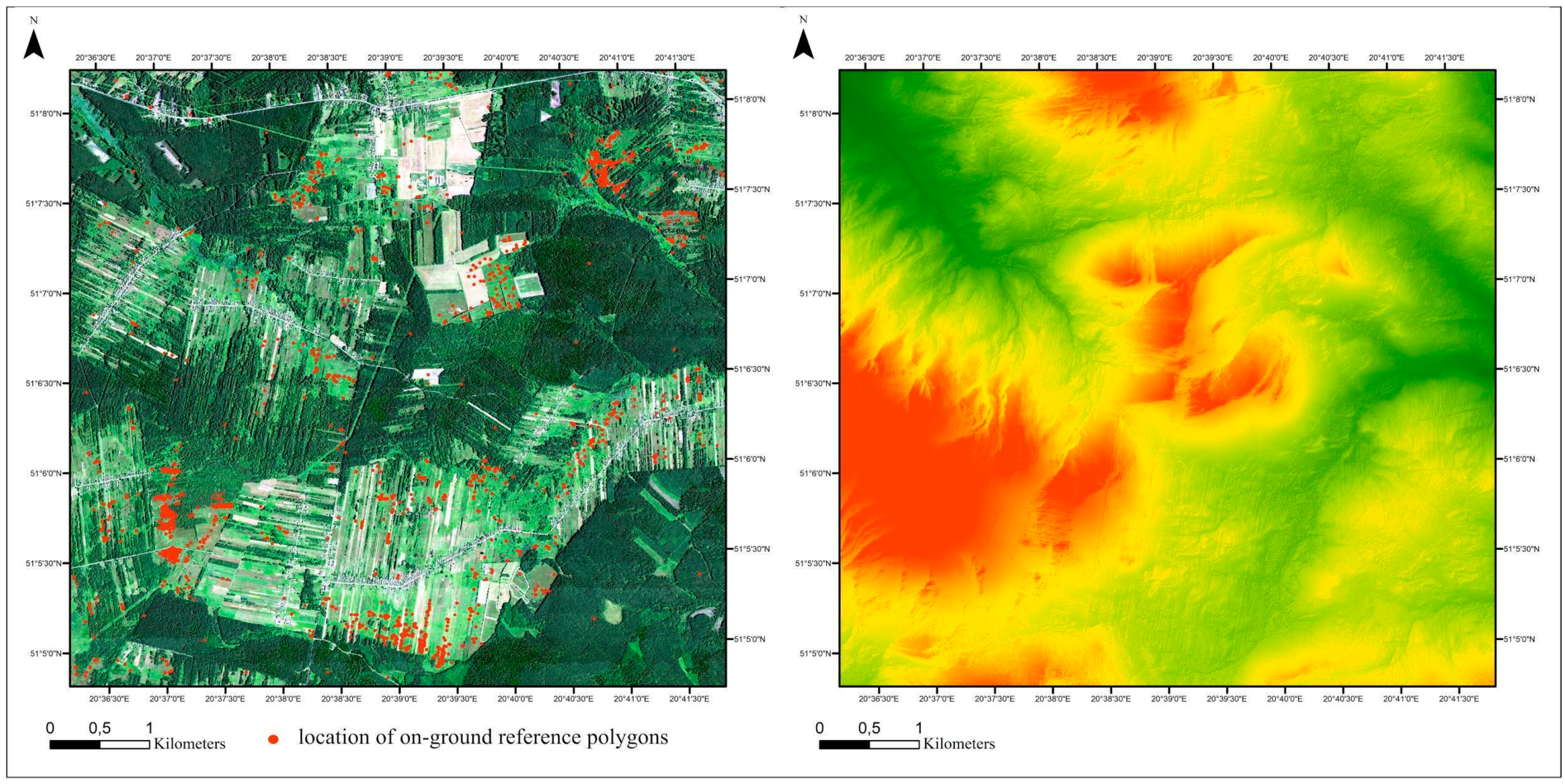
2.1. Study Area and Object of the Study
2.2. Data Acquisition
2.2.1. On-Ground Reference Data
2.2.2. Remote-Sensing Data Acquisition
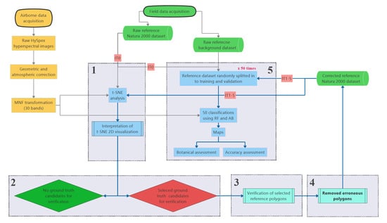
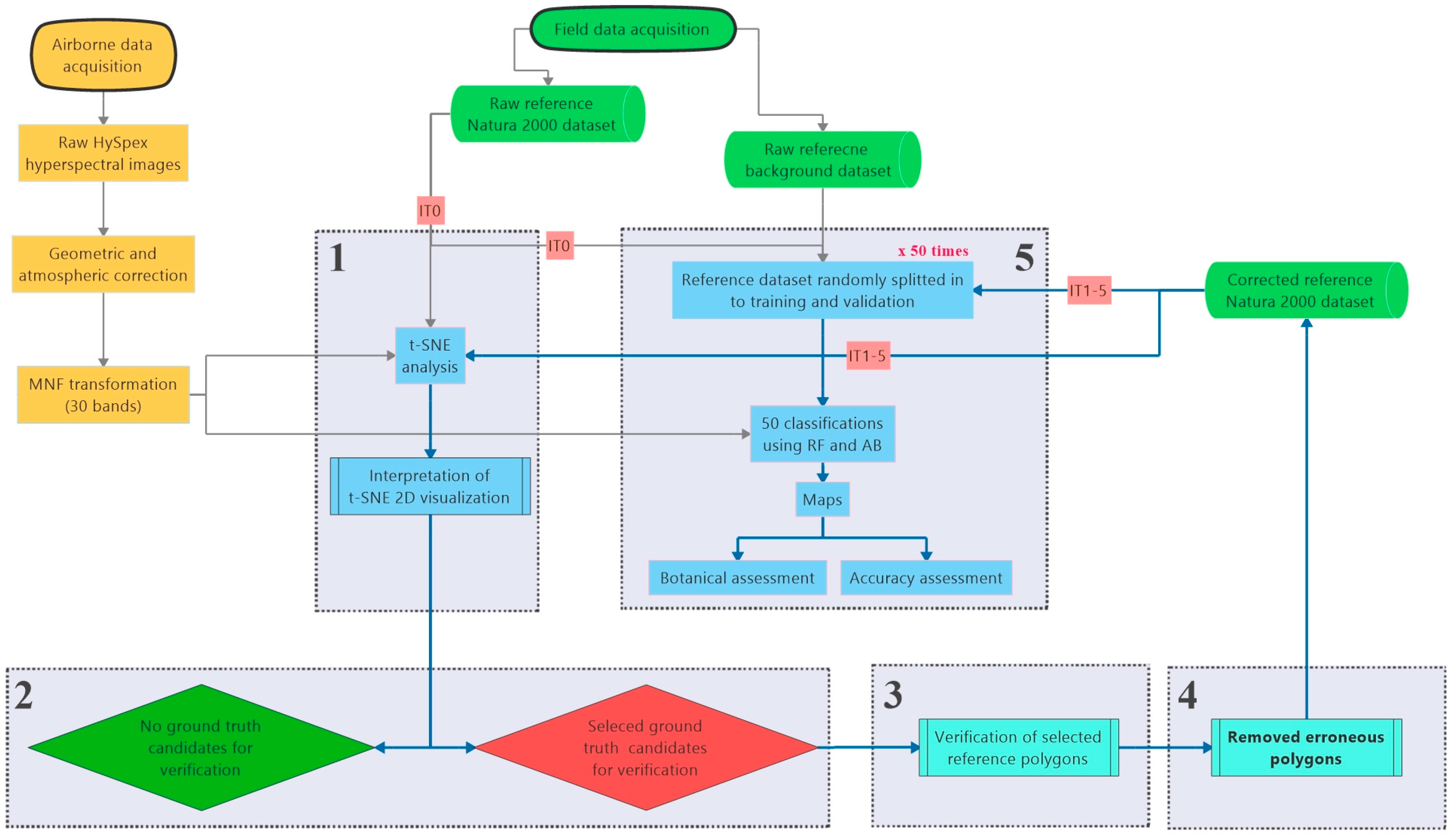
2.3. Analysis Workflow
2.3.1. Generating t-SNE Based Visualization of Reference Dataset
2.3.2. Visual Interpretation of t-SNE Plots to Select Candidate Polygons for Verification
2.3.3. Verification of Candidate Ground Truth Polygons and Removal of Erroneous Reference
2.3.4. Classification and Validation
2.3.5. Botanical Assessment of Classification Products (Maps)
3. Results
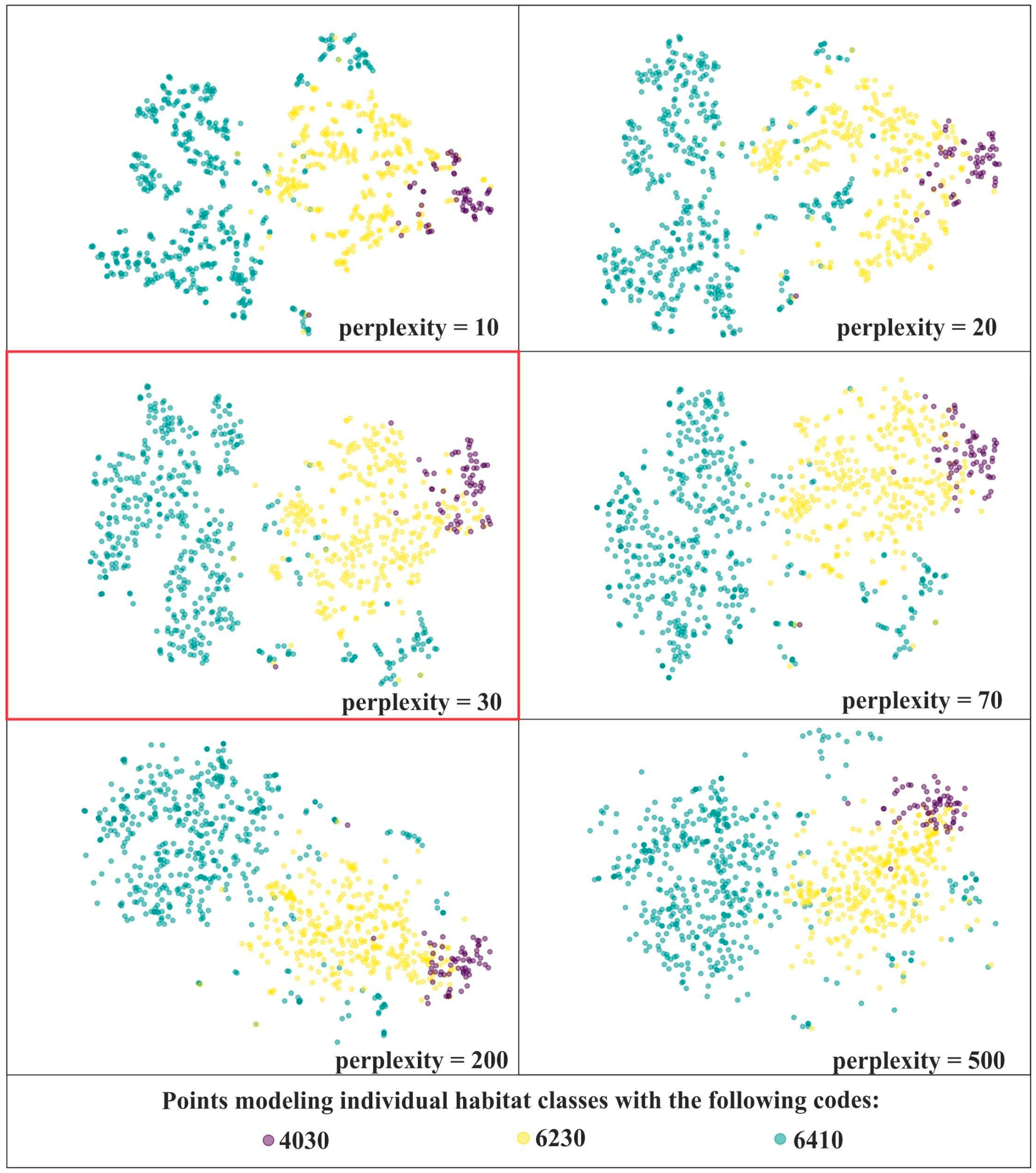
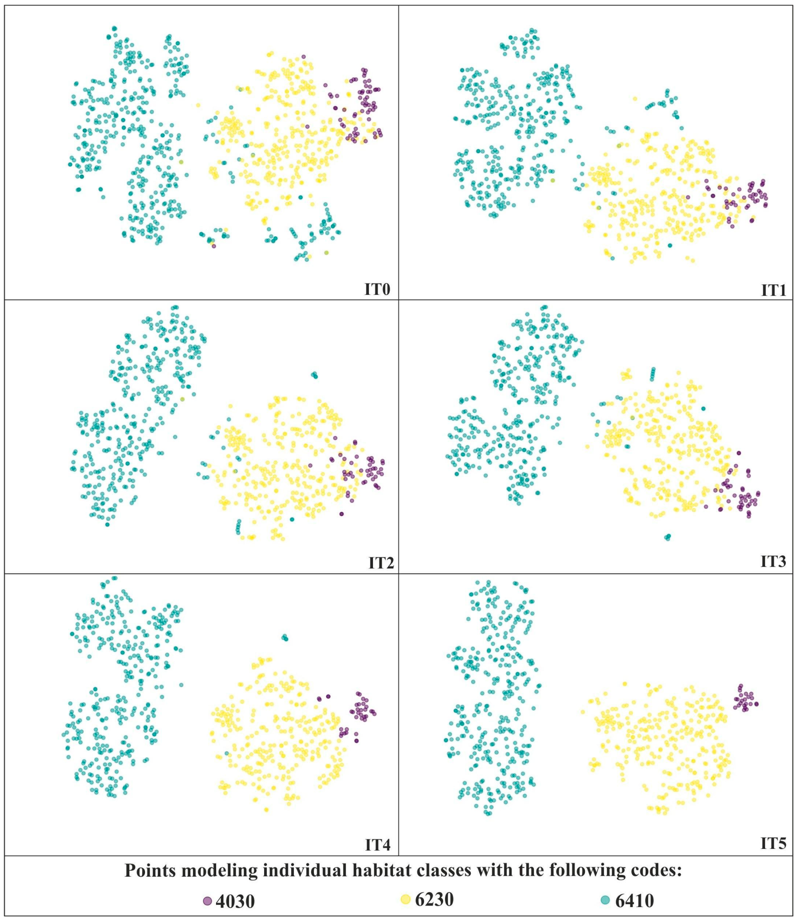
3.1. Results of the t-SNE Analysis
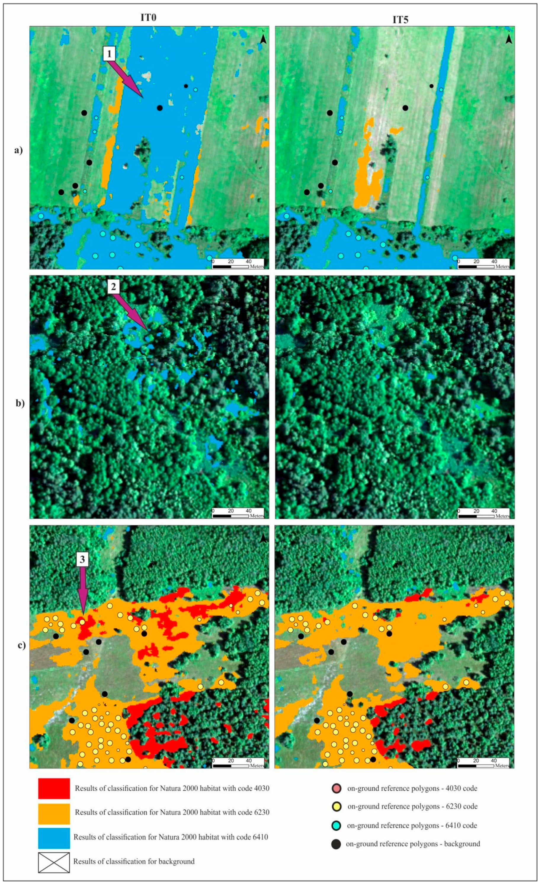
3.2. Effectiveness of Our Workflow
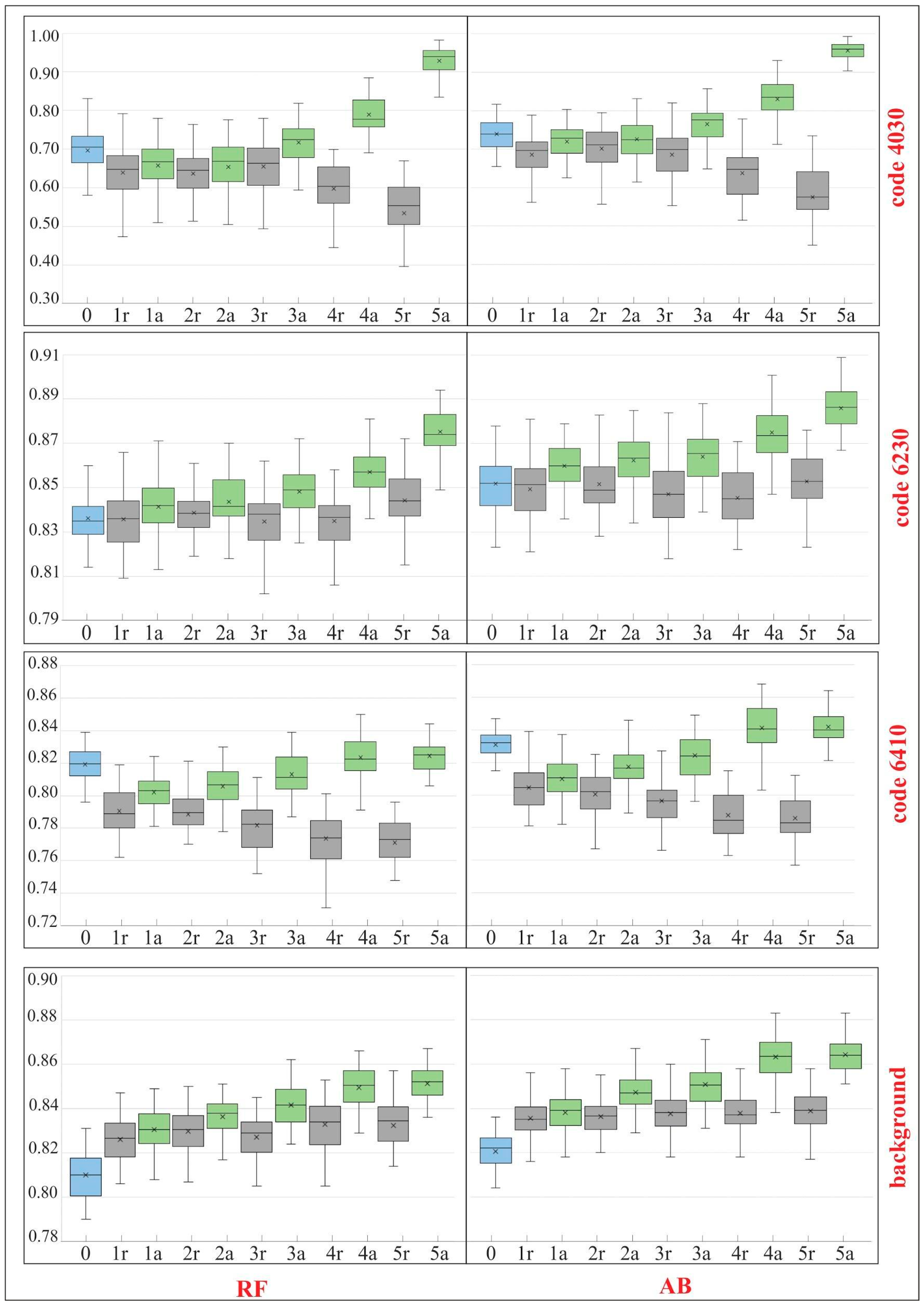
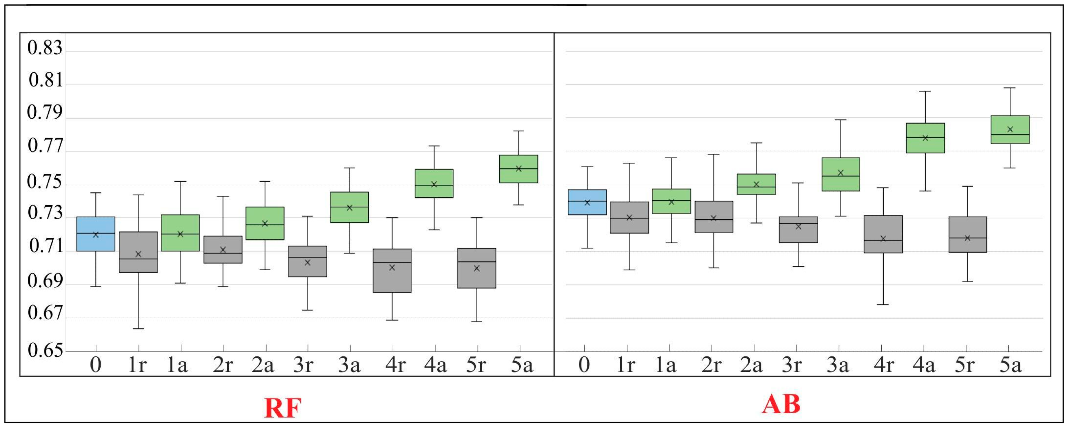
3.3. Results of the RF and AB Classification Obtained at Various Stages of the On-Ground Reference Dataset Modification
3.4. Interpretation of Results
4. Discussion
4.1. Evaluation of the t-SNE Algorithm Applicability to the Improvement of the On-Ground Reference Dataset Quality
4.2. Impact of the On-Ground Reference Dataset Modification on the Results of Classification of Selected Natura 2000 Habitats
5. Conclusions
Author Contributions
Funding
Conflicts of Interest
References
- Foody, G.M.; Pal, M.; Rocchini, D.; Garzon-Lopez, C.; Bastin, L. The sensitivity of mapping methods to reference data quality: Training supervised image classifications with imperfect reference data. ISPRS Int. J. Geo-Inf. 2016, 5, 199. [Google Scholar] [CrossRef] [Green Version]
- Lillesand, T.M.; Kiefer, R.W. Remote Sensing and Image Interpretation, 3rd ed.; John Wiley & Sons: New York, NY, USA, 1994. [Google Scholar]
- Mellor, A.; Boukir, S.; Haywood, A.; Jones, S. Exploring issues of training data imbalance and mislabelling on random forest performance for large area land cover classification using the ensemble margin. ISPRS J. Photogramm. Remote Sens. 2015, 105, 155–168. [Google Scholar] [CrossRef]
- Costa, H.; Foody, G.M.; Jiménez, S.; Silva, L. Impacts of species misidentification on species distribution modeling with presence-only data. ISPRS Int. J. Geo-Inf. 2015, 4, 2496–2518. [Google Scholar] [CrossRef] [Green Version]
- Mather, P.M. Computer Processing of Remotely-Sensed Images: An Introduction, 3rd ed.; John Wiley and Sons: Chichester, UK, 2004. [Google Scholar]
- Congalton, R.G.; Green, K. Assessing the Accuracy of Remotely Sensed Data: Principles and Practices; CRC Press: Boca Raton, FL, USA, 2008. [Google Scholar]
- Foody, G.M.; Mathur, A.; Sanchez-Hernandez, C.; Boyd, D.S. Training set size requirements for the classification of a specific class. Remote Sens. Environ. 2006, 104, 1–14. [Google Scholar] [CrossRef]
- Ge, Y.; Bai, H.; Wang, J.; Cao, F. Assessing the quality of training data in the supervised classification of remotely sensed imagery: A correlation analysis. J. Spat. Sci. 2012, 57, 135–152. [Google Scholar] [CrossRef]
- Pelletier, C.; Valero, S.; Inglada, J.; Champion, N.; Sicre, C.M.; Dedieu, G. Effect of training class label noise on classification performances for land cover mapping with satellite image time series. Remote Sens. 2017, 9, 173. [Google Scholar] [CrossRef] [Green Version]
- Guo, L. Margin Framework for Ensemble Classifiers. Application to Remote Sensing Data. Ph.D. Thesis, University of Bordeaux, Bordeaux, France, 2011. [Google Scholar]
- Kopeć, K.; Wylazłowska, J.; Niedzielko, J.; Jarocińska, A.; Borzuchowski, J.; Piórkowski, H.; Błońska, A.; Niedzielko, M.; Halladin-Dąbrowska, A.; Michalska-Hejduk, D.; et al. Auxiliary work in WP3 under the programme “Natural Environment, Agriculture and Forestry” BIOSTRATEG II.: The innovative approach supporting monitoring of non-forest Natura 2000 habitats, using remote sensing methods (HabitARS). Unpublished work.
- Ramaswamy, S.; Rastogi, R.; Shim KAIST, K. Efficient algorithms for mining outliers from large data sets. In Proceedings of the 2000 ACM SIGMOD International Conference on Management of Data, Dallas, TX, USA, 15–18 May 2000. [Google Scholar]
- Liu, F.T.; Ting, K.M.; Zhou, Z.-H. Isolation-based anomaly detection. ACM Trans. Knowl. Discov. Data 2012, 6, 3. [Google Scholar] [CrossRef]
- Breunig, M.M.; Kriegel, H.-P.; Ng, R.T.; Sander, J. LOF: Identifying density-based local outliers. In Proceedings of the 2000 ACM SIGMOD International Conference on Management of Data, Dallas, TX, USA, 15–18 May 2000. [Google Scholar]
- Büschenfeld, T.; Ostermann, J. Automatic refinement of training data for classification of satellite imagery. In Proceedings of the PISPRS Annals of the Photogrammetry, Remote Sensing and Spatial Information Sciences, Melbourne, Australia, 25 August–1 September 2012. [Google Scholar]
- Kavzoglu, T. Increasing the accuracy of neural network classification using refined training data. Environ. Model. Softw. 2009, 24, 850–858. [Google Scholar] [CrossRef]
- Mather, P.M. Computational Methods of Multivariate Analysis in Physical Geography; John Wiley and Sons: Chichester, UK, 1976. [Google Scholar]
- Van Der Maaten, L.; Hinton, G. Visualizing data using t-SNE. J. Mach. Learn. Res. 2008, 9, 2579–2605. [Google Scholar]
- Zhang, J.; Chen, L.; Zhuo, L.; Liang, X.; Li, J. An efficient hyperspectral image retrieval method: Deep spectral-spatial feature extraction with DCGAN and dimensionality reduction using t-SNE-based NM hashing. Remote Sens. 2018, 10, 271. [Google Scholar] [CrossRef] [Green Version]
- Zhong, Z.; Li, J.; Ma, L.; Jiang, H.; Zhao, H. Deep residual networks for hyperspectral image classification. In Proceedings of the IEEE International Geoscience and Remote Sensing Symposium (IGARSS), Fort Worth, TX, USA, 23–28 July 2017. [Google Scholar]
- Dai, X.; Guo, S.; Li, X. Novel hyperspectral image classification method based on the t-SNE and AdaBoost algorithms. In Proceedings of the Association of American Geographers Annual Meeting, New Orleans, LA, USA, 10–14 April 2018. [Google Scholar]
- Zhang, L.; Zhong, Y.; Huang, B.; Gong, J.; Li, P. Dimensionality reduction based on clonal selection for hyperspectral imagery. IEEE Trans. Geosci. Remote Sens. 2007, 45, 4172–4186. [Google Scholar] [CrossRef]
- Halladin-Dąbrowska, A.; Kania, A.; Sławik, Ł.; Niedzielko, J.; Borzuchowski, J.; Wylazłowska, J.; Michalska-Hejduka, D.; Kopeć, D. The t-SNE Machine Learning Algorithm As A Novel Tool Supporting The Classification Of Non-forest Natura 2000 Habitats. In Proceedings of the Sixth International Conference on Remote Sensing and Geoinformation of Environment, Paphos, Cyprus, 26–29 March 2018. [Google Scholar]
- Kania, A. Interactive tool for real-time delivery of remote sensing based vegetation maps and support of botanical data collection. In Proceedings of the 10th International Conference on Ecological Informatics. Translating Ecological Data into Knowledge and Decisions in a Rapidly Changing World, Jena, Germany, 24–28 September 2018; pp. 59–60. [Google Scholar]
- Chan, W.; Spanhove, T.; Ma, J.; Vanden Borre, J.; Paelinckx, D.; Canters, F. Natura 2000 habitat identification and conservation status assessment with superresolution enhanced hyperspectral (CHRIS/PROBA) imagery. In Proceedings of the GEOBIA 2010-Geographic Object-Based Image Analysis, Ghent, Belgium, 29 June–2 July 2010. [Google Scholar]
- Folleco, A.; Khoshgoftaar, T.M.; Hulse, J.; Van Bullard, L. Identifying learners robust to low quality data. In Proceedings of the IEEE International Conference on Information Reuse and Integration, Las Vegas, NV, USA, 13–15 July 2008. [Google Scholar] [CrossRef]
- Rodriguez-Galiano, V.; Ghimire, B.; Rogan, J.; Chica-Olmo, M.; Rigol-Sanchez, J. An assessment of the effectiveness of a random forest classifier for land-cover classification. ISPRS J. Photogramm. Remote Sens. 2012, 67, 93–104. [Google Scholar] [CrossRef]
- Sun, B.; Chen, S.; Wang, J.; Chen, H. A robust multi-class AdaBoost algorithm for mislabeled noisy data. Knowl.-Based Syst. 2016, 102, 87–102. [Google Scholar] [CrossRef]
- Banfield, R.E.; Hall, L.O.; Bowyer, K.W.; Kegelmeyer, W.P. A Comparison of decision tree ensemble creation techniques. IEEE Trans. Pattern. Anal. Mach. Intell. 2007, 29, 173–180. [Google Scholar] [CrossRef]
- Dietterich, T.G. An experimental comparison of three methods for constructing ensembles of decision trees: Bagging, boosting, and randomization. Mach. Learn. 2000, 40, 139–157. [Google Scholar] [CrossRef]
- Sławik, Ł.; Niedzielko, J.; Kania, A.; Piórkowski, H.; Kopeć, D. Multiple flights or single flight instrument fusion of hyperspectral and ALS data? A comparison of their performance for vegetation mapping. Remote Sens. 2019, 11, 970. [Google Scholar] [CrossRef] [Green Version]
- ENVI API Programming Guide. Harris Geospatial Solutions Documentation Center. Available online: http://www.harrisgeospatial.com/docs/ProgrammingGuideIntroduction.html (accessed on 8 February 2019).
- Millard, K.; Richardson, M. Wetland mapping with LiDAR derivatives, SAR polarimetric decompositions, and LiDAR-SAR fusion using a random forest classifier. Can. J. Remote Sens. 2013, 39, 290–307. [Google Scholar] [CrossRef]
- Van Der Maaten, L.; Courville, A.; Fergus, R.; Manning, C. Accelerating t-SNE using tree-based algorithms. J Mach. Learn. Res. 2014, 15, 3221–3245. [Google Scholar]
- Vegetation Classification Studio Software, Version 2.13/hb. Available online: http://www.definity.pl/vcs (accessed on 5 September 2019).
- Cohen, J. A Coefficient of Agreement for Nominal Scales. Educ. Psychol. Meas. 1960, 20, 37–46. [Google Scholar] [CrossRef]
- Gonçalves, J.; Henriques, R.; Alves, P.; Sousa-Silva, R.; Monteiro, A.T.; Lomba, Â.; Marcos, B.; Honrado, J. Evaluating an unmanned aerial vehicle-based approach for assessing habitat extent and condition in fine-scale early successional mountain mosaics. Appl. Veg. Sci. 2016, 19, 132–146. [Google Scholar] [CrossRef] [Green Version]
- Buck, O.; Millán, V.E.G.; Klink, A.; Pakzad, K. Using information layers for mapping grassland habitat distribution at local to regional scales. Int. J. Appl. Earth Obs. Geoinf. 2015, 37, 83–89. [Google Scholar] [CrossRef]
- Stenzel, S.; Feilhauer, H.; Mack, B.; Metz, A.; Schmidtlein, S. Remote sensing of scattered natura 2000 habitats using a one-class classifier. Int. J. Appl. Earth Obs. Geoinf. 2014, 33, 211–217. [Google Scholar] [CrossRef]
- Schuster, C.; Schmidt, T.; Conrad, C.; Kleinschmit, B.; Förster, M. Grassland habitat mapping by intra-annual time series analysis -Comparison of RapidEye and TerraSAR-X satellite data. Int. J. Appl. Earth Obs. Geoinf. 2015, 34, 25–34. [Google Scholar] [CrossRef]
- Zlinszky, A.; Schroiff, A.; Kania, A.; Deák, B.; Mücke, W.; Vári, Á.; Székely, B.; Pfeifer, N. Categorizing grassland vegetation with full-waveform airborne laser scanning: A feasibility study for detecting natura 2000 habitat types. Remote Sens. 2014, 6, 8056–8087. [Google Scholar] [CrossRef] [Green Version]
- Breiman, L. Random Forests. Mach. Learn. 2001, 45, 5–32. [Google Scholar] [CrossRef] [Green Version]
- Agjee, N.H.; Mutanga, O.; Peerbhay, K.; Ismail, R. The Impact of Simulated Spectral Noise on Random Forest and Oblique Random Forest Classification Performance. J. Spectrosc. 2018, 2018, 8316918. [Google Scholar] [CrossRef] [Green Version]


| Analyzed Characteristic | Natura 2000 Habitat Code 4030 | Natura 2000 Habitat Code 6230 | Natura 2000 Habitat Code 6410 |
|---|---|---|---|
| Species richness and dominant species diversity between habitat patches | low | medium | very high |
| Variability in dominant species composition within a habitat patch between different years | low | low | very high |
| Dominant species composition similarity with other analyzed types of Natura 2000 habitats | some patches very similar to Natura 2000 Habitat with code 6230 | some patches very similar to Natura 2000 Habitat with code 4030; sporadically small similarity to Natura 2000 Habitat with code 6410 | sporadically small similarity to Natura 2000 Habitat with code 6230 |
| Dominant species composition similarity with other types of vegetation that may form the background | none | small | relatively high |
| Possibility of photointerpretation on high-resolution orthophoto maps in natural colors (RGB) | partial | none | none |
| Year of Data Acquisition | Number of Established Polygons for Each Natura 2000 Habitat and from Background Class | ||||
|---|---|---|---|---|---|
| Code 4030 | Code 6230 | Code 6410 | Background | Total | |
| 2016 | 0 | 169 | 158 | 43 | 370 |
| 2017 | 63 | 157 | 314 | 572 | 1106 |
| Total | 63 | 326 | 472 | 615 | 1476 |
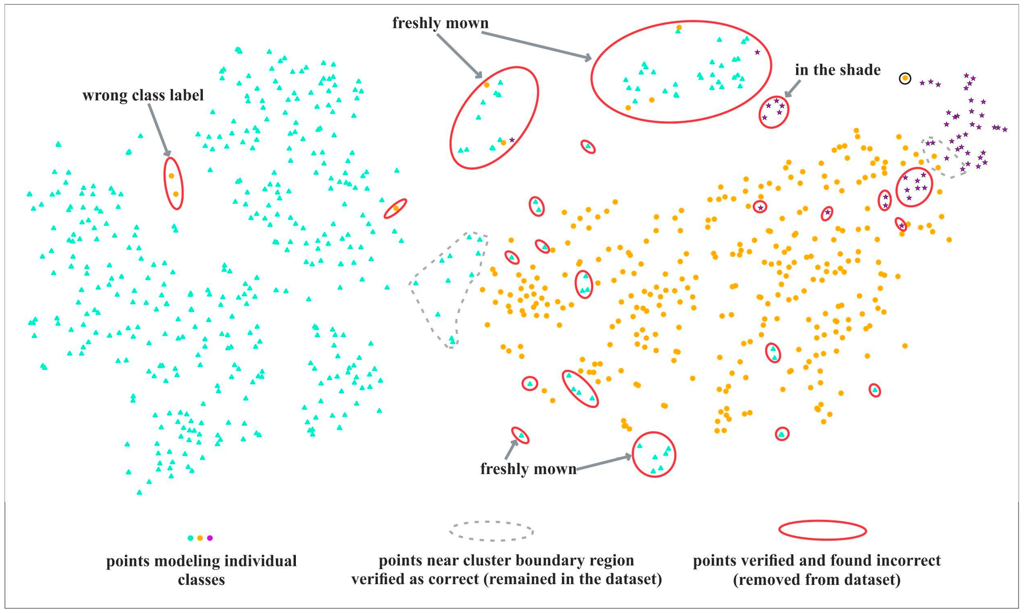
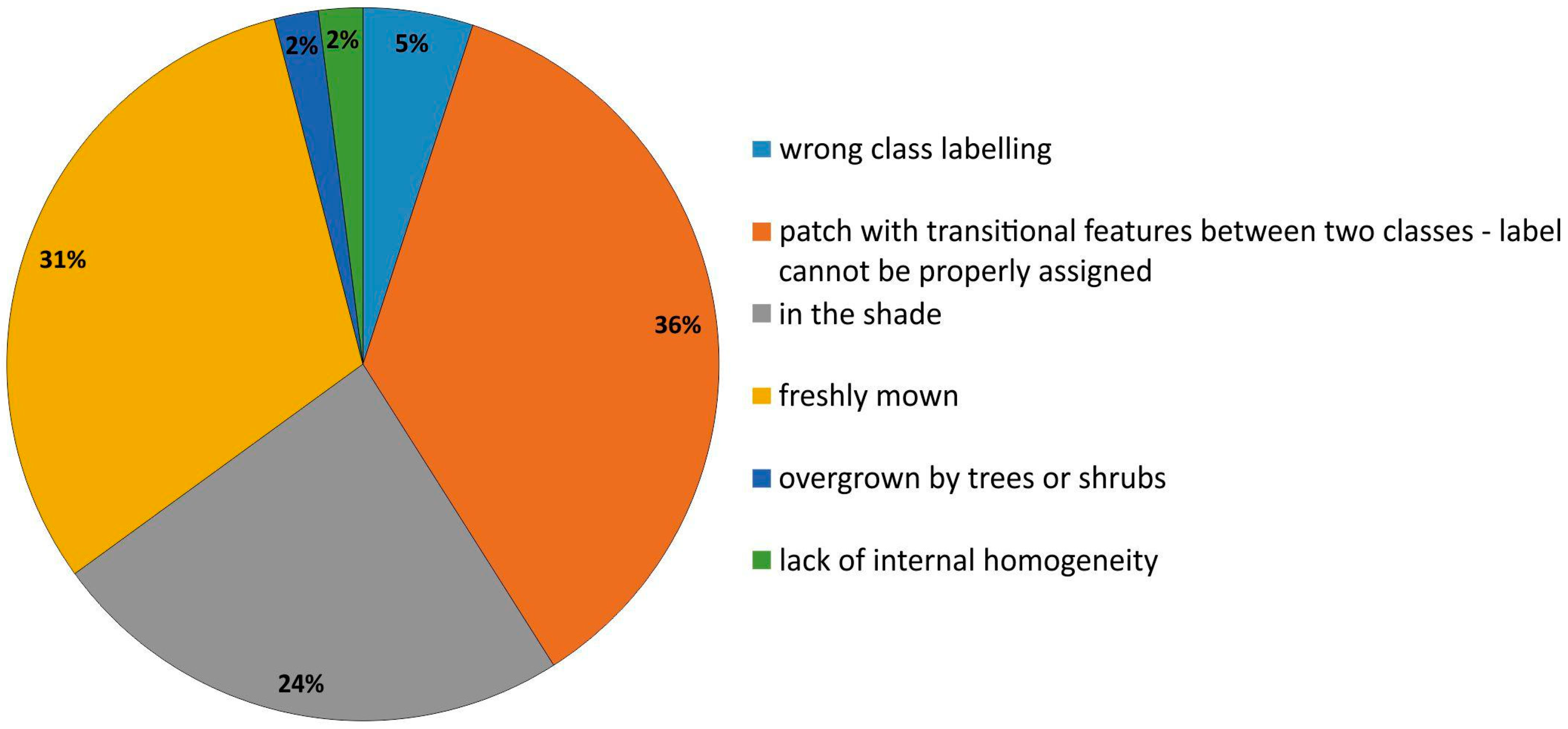
| Visual Artifact/Pattern on t-SNE Plot | Definition of a Given Type of Artifact | Possible Cause/Effect/Rationale in Reference Database |
|---|---|---|
 | Single elements of differing class among a dense cluster of another class | Wrong/switched class label |
| Atypical and/or rare case of polygon, very similar in its properties to another class | ||
  | Element of differing class on the boundary region of different class cluster | Wrong/switched class label |
| Might be a correct reference item, with a similar species composition or structure to another class | ||
| The type of boundary—smooth or clearly defined—shall correspond to the nature of the difference between vegetation classes. Smooth transition with similarly-spaced points on class boundary indicates smooth, gradual transition between vegetation classes. Clearly distinct boundaries with visible spacing between clusters indicates vegetation classes with clearly differing spectral properties. If boundary type on t-SNE plots is different from expected—a closer analysis might be suggested to understand the reason for the difference. | ||
 | Small clusters of homogeneous class formed outside of main/dominant cluster | Could be valid subclasses within the class |
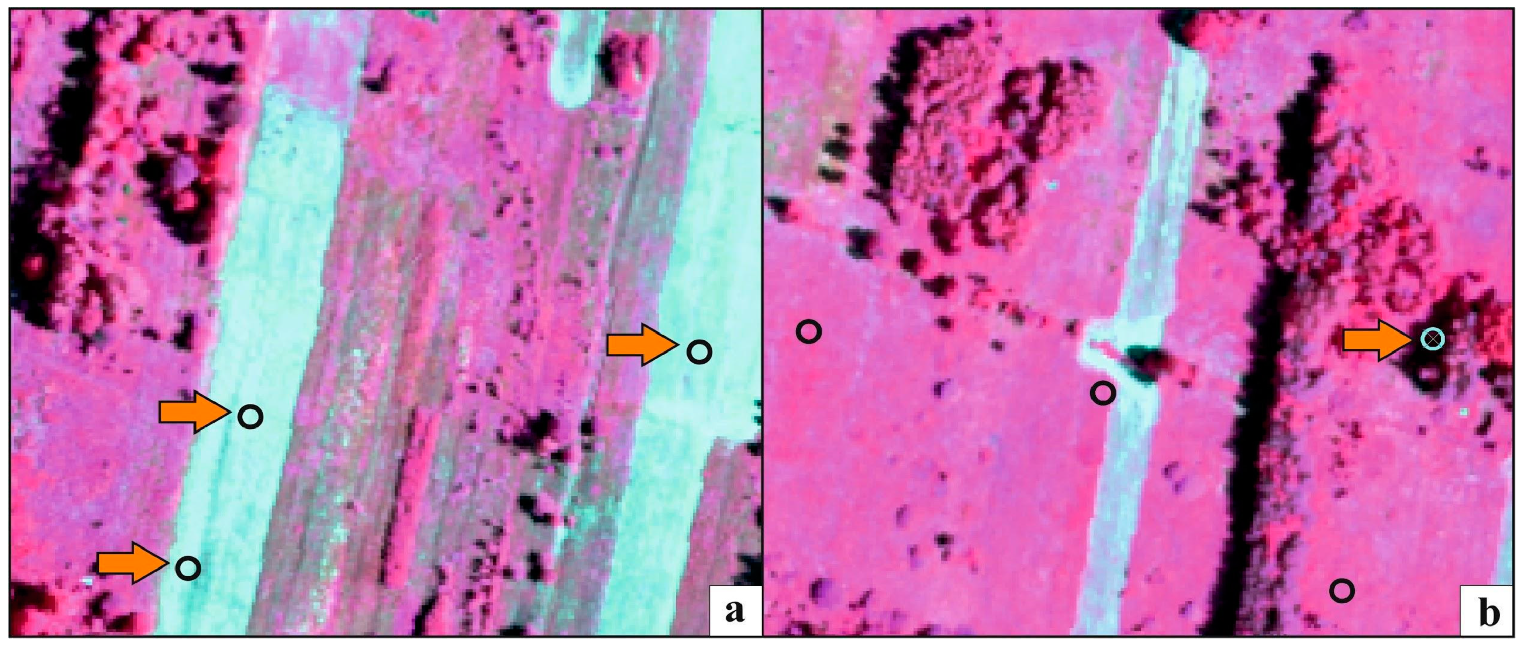
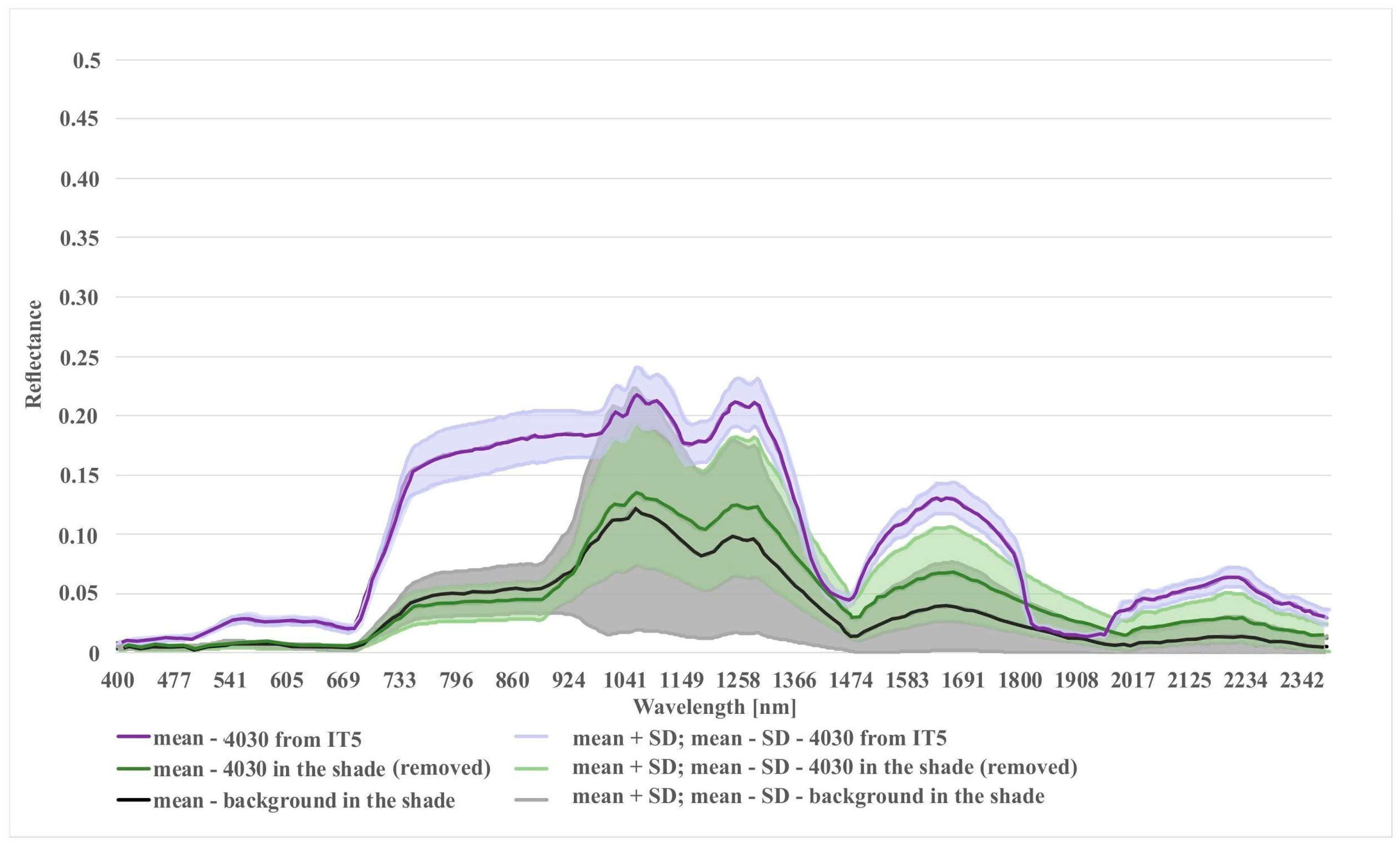
| Atypical cases (in our analysis many of them were due to being in the shadow) | ||
 | Small, and clearly disjoint clusters composed of multiple classes | Might hint at a subclass, often having a common characteristic (between multiple classes); typical case is polygons (of potentially varied classes) located in the shade |
| Class Name/Natura 2000 Code | The Number of On-Ground Reference Polygon Errors Identified and Removed in Iterations IT1–IT5 | Total Errors Removed/Total Polygons Before Workflow (Raw Dataset) | |||||
|---|---|---|---|---|---|---|---|
| IT0 | IT1 | IT2 | IT3 | IT4 | IT5 | ||
| 4030 | 0 | 18 | 0 | 1 | 8 | 13 | 40/63 |
| 6230 | 0 | 24 | 2 | 12 | 9 | 0 | 47/326 |
| 6410 | 0 | 91 | 12 | 3 | 18 | 5 | 129/472 |
| Background 1 | 0 | 0 | 0 | 0 | 0 | 0 | 0/615 |
| Total | 0 | 133 | 14 | 16 | 35 | 18 | 216/1476 |
| On-Ground Reference Data [%]: RF/AB | ||||||
|---|---|---|---|---|---|---|
| Iteration | Class | 4030 | 6230 | 6410 | background | PA [%] |
| IT0 (raw, unmodified reference database) | 4030 | 83/87 | 7/4 | 0/0 | 0/0 | 62/72 |
| 6230 | 17/13 | 85/86 | 1/1 | 6/5 | 82/86 | |
| 6410 | 0/0 | 0/1 | 80/79 | 12/10 | 83/88 | |
| background | 0/0 | 8/9 | 19/20 | 81/85 | 82/79 | |
| UA [%] | 83/87 | 85/86 | 80/79 | 81/85 | ||
| IT5 (after our workflow) | 4030 | 100/99 | 0/0 | 0/0 | 0/0 | 87/95 |
| 6230 | 0/1 | 90/87 | 0/1 | 5/4 | 87/90 | |
| 6410 | 0/0 | 0/0 | 80/81 | 8/7 | 86/88 | |
| background | 0/0 | 10/13 | 20/19 | 87/89 | 85/84 | |
| UA [%] | 100/99 | 90/87 | 80/81 | 87/89 | ||
© 2019 by the authors. Licensee MDPI, Basel, Switzerland. This article is an open access article distributed under the terms and conditions of the Creative Commons Attribution (CC BY) license (http://creativecommons.org/licenses/by/4.0/).
Share and Cite
Halladin-Dąbrowska, A.; Kania, A.; Kopeć, D. The t-SNE Algorithm as a Tool to Improve the Quality of Reference Data Used in Accurate Mapping of Heterogeneous Non-Forest Vegetation. Remote Sens. 2020, 12, 39. https://0-doi-org.brum.beds.ac.uk/10.3390/rs12010039
Halladin-Dąbrowska A, Kania A, Kopeć D. The t-SNE Algorithm as a Tool to Improve the Quality of Reference Data Used in Accurate Mapping of Heterogeneous Non-Forest Vegetation. Remote Sensing. 2020; 12(1):39. https://0-doi-org.brum.beds.ac.uk/10.3390/rs12010039
Chicago/Turabian StyleHalladin-Dąbrowska, Anna, Adam Kania, and Dominik Kopeć. 2020. "The t-SNE Algorithm as a Tool to Improve the Quality of Reference Data Used in Accurate Mapping of Heterogeneous Non-Forest Vegetation" Remote Sensing 12, no. 1: 39. https://0-doi-org.brum.beds.ac.uk/10.3390/rs12010039