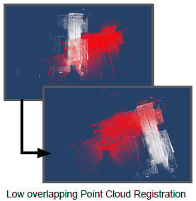
Low Overlapping Point Cloud Registration Using Line Features Detection


National Institute of Advanced Industrial Science and Technology, Tokyo 135-0064, Japan
*
Author to whom correspondence should be addressed.
†
Current address: College of Science and Engineering, The University of Edinburgh, Edinburgh, UK.
Remote Sens. 2020, 12(1), 61; https://0-doi-org.brum.beds.ac.uk/10.3390/rs12010061
Submission received: 26 November 2019
/
Revised: 17 December 2019
/
Accepted: 19 December 2019
/
Published: 23 December 2019
(This article belongs to the Special Issue Point Cloud Processing in Remote Sensing)
Abstract
:Modern robotic exploratory strategies assume multi-agent cooperation that raises a need for an effective exchange of acquired scans of the environment with the absence of a reliable global positioning system. In such situations, agents compare the scans of the outside world to determine if they overlap in some region, and if they do so, they determine the right matching between them. The process of matching multiple point-cloud scans is called point-cloud registration. Using the existing point-cloud registration approaches, a good match between any two-point-clouds is achieved if and only if there exists a large overlap between them, however, this limits the advantage of using multiple robots, for instance, for time-effective 3D mapping. Hence, a point-cloud registration approach is highly desirable if it can work with low overlapping scans. This work proposes a novel solution for the point-cloud registration problem with a very low overlapping area between the two scans. In doing so, no initial relative positions of the point-clouds are assumed. Most of the state-of-the-art point-cloud registration approaches iteratively match keypoints in the scans, which is computationally expensive. In contrast to the traditional approaches, a more efficient line-features-based point-cloud registration approach is proposed in this work. This approach, besides reducing the computational cost, avoids the problem of high false-positive rate of existing keypoint detection algorithms, which becomes especially significant in low overlapping point-cloud registration. The effectiveness of the proposed approach is demonstrated with the help of experiments.
1. Introduction
Point cloud registration is the process of aligning two or more point-clouds by estimating the relative transformation between them. Point cloud registration is an important part of computer vision algorithms, 3D mapping and 3D scene reconstruction, to name a few. Three-dimensional mapping of the surrounding environment using a multi-robot system is an established research area. A multi-robot system has the potential to improve the efficiency of 3D mapping over a single robot. Authors in [1,2] presented new approaches for multi-robot martial cave explorations. Among the novel concepts in autonomous robotics explorations presented in their work is sophisticated coordination autonomy. This requires peer-to-peer communication between agents that allows scouting rovers to explore beyond the reach of their telecommunication resources. In case two agents meet at a sufficient distance from each other, either by chance or deliberately, the exchange of information about explored environment should happen reliably and effectively. Assuming no global localization system is available, it is tempting to merge the world models based on areas of their intersection. This problem becomes especially complex if the state-of-the-art LiDAR mapping technique is used. Even though an extensive research in the area of point-cloud registration has been done (see Section 2), the case where the ratio of an overlapping area is significantly small, has not yet been explored. Hence, this work proposes an approach for point-cloud registration with an overlapping area between two scans as low as 20% (As suggested by our experiments).
Our proposed approach assumes the existence of straight edges in the 3D scans, which in most environments is a reasonable assumption. In offices, one can find desks, monitors, chair legs, etc. In urban areas, such objects include buildings, pavements, road signs, lamps or in the case of the outdoors such objects include trees, branches, sharp rocks, karst formations in caves, etc. We propose the use of edge detection followed by Hough transform to detect lines in the two-point-clouds which need to be merged.
For an arbitrary area of a point-cloud scan P, the set of lines serves as a global descriptor of A provided . Generally speaking, in order to find a transformation, we do not need to run exhaustive calculations to create and pair-wise match the local descriptors of keypoints in two scans as proposed in [3] or in other state-of-the-art point-cloud registration approaches [4]. In contrast, our work proposes the use of a trial-and-error method, where the evaluation of a match is much more efficient. The key idea is to prune the search space by finding the transformation parameters one by one rather than searching throughout the whole parameter space. This is achieved by performing the matching phase in the following three main steps.
All the three matchings are performed by minimizing a fitness function based on pairwise dot products between directional vectors of lines detected in the two given scans. In parallel with this, the following two assumptions are made.
- The gravity vector is known prior to running our outline and, hence, only rotation around z-axis is required to find correct rotations of the scans relative to each other. This is a reasonable assumption in the majority of real-world scenarios because all the LiDAR scanners are equipped with a gyroscope sensor and their output is correctly aligned with gravity vector pointing in the negative direction of z-axis.
- No scans need to be translated in a vertical direction. This assumption greatly simplifies the presentation of the idea and derivation of mathematical formulas at the cost of its applicability to a larger problem domain. We aim to motivate the more general solution, which allows translation over all three x, y and z-axes and can be implemented as an extension to this work.
We believe that the results, even in the presence of the above assumptions, are of a real-world use for a number of problems, e.g., merging indoor scans of the same floor in a building or a simple outdoor environment with a straight ground.
The rest of the paper is organized as follows. Section 2 discusses the related work. In Section 3, our proposed point-cloud registration approach using line features is presented. Section 4 presents the experimental evaluation of the proposed approach while Section 5 discusses in detail the proposed approach’s parameters tuning. Section 6 concludes our paper by highlighting some of the limitations of this work and discussing interesting future directions.
2. Related Work
To the best of our knowledge, very little work on the problem of merging two-point-clouds, where the overlapping area is much smaller than any of their corresponding sizes, has been done. One of the most related work in this area has been done by Jiří Hörner in [3]. Their method uses a similar approach to the point-cloud registration problem and has recently gained a lot of attention in research [5,6], i.e., they presented an algorithm based on matching keypoints with calculated corresponding geometrical descriptors around them. This explicitly introduces the general assumption of a point-cloud registration problem; that the size of an overlapping area is very large and only a minor correction in translation and rotation is sought [4]. Generally, the solution in a high overlapping point-cloud consists of keypoints detection [7,8,9], descriptors calculation [10,11,12] around each of the keypoints and running an Iterative Closest Point (ICP) algorithm [13,14] to find a transformation that pair-wise matches the individual descriptors. When the overlapping area is small, as in our case, it is difficult to reliably find the matching keypoints in the two-point-clouds, which is an essential step in almost all of the existing point-cloud registration approaches. Besides, there exists two more problems with the ICP algorithm being used by majority of the above discussed works. (1) ICP is an iterative algorithm and the quality of results strongly depends on an initial configuration, which in our case might be too far from the one leading to a reasonable solution since we do not assume any initial alignment (2) the convergence accuracy is strongly correlated to the ratio of an overlapping area with the value of 50% being critical [15].
To tackle this problem, several approaches have been suggested. For instance, Ref. [16] explores correlations between Extended Gaussian Images [17] in Fourier Transform domain to find a crude alignment, which is later refined by ICP and accepts as low as 45% partial overlap. Go-ICP [18] uses a branch-and-bound scheme to search 3D motion space and guarantees to return globally optimal solutions disregarding an initial configuration. As pointed out by [19], this method becomes computationally too complex if the overlap gets below 70%. Moreover, Go-ICP has been tested only on small point-cloud scans and the scalability is unlikely due to its complexity. Super 4PCS [20] aims to reach globally optimal solutions as well. According to experiments in [19], it can produce reasonable results for scans with overlapping ratios as low as 30%, however, it suffers from instability, i.e., variance of accuracy of results is high. [19] proposes a method to use hidden Markov random fields to capture the fact that most of the time, the non-correspondences appear close to each other. The comparison of [19] with Go-ICP [18] and Super 4PCS [20] suggests only a negligible improvement over minimum ratio of an overlap that is required for the algorithm to work accurately. However, the results show that the approach benefits from the greater stability compared to the other two methods, i.e., it has lower variance in its results.
Wu et al. [15] proposed a modified version of the registration method with the use of the LM-ICP method which can converge with lower overlapping ratios between point-clouds and demonstrated the approach on cases with 37% and 44% overlapping ratios. Their method evaluates pair-wise similarities between sampled points in two given point-clouds by calculating mean and Gaussian curvatures of local surrounding surfaces. Because of an exponential rise of the number of possible pairs, this method is not scalable to larger, possibly indoor or outdoor environments.
Other approaches to the problem include optimization via genetic algorithms [21,22,23] and demonstrate good results for as low as 50% overlap between two-point-clouds. However, their performance has been only evaluated on registration of CAD models and their generalization to real-world scene registration is rather questionable due to the problems of local optima and of a slow convergence time with an increasing amount of data.
The closest approach to our work is [24] where planar surfaces are detected via RANSAC. As opposed to our idea, the planar surfaces are then intersected obtaining keypoints around which descriptors are calculated, which is the main drawback of the work due to the complexity of descriptor computation. A geometric constrained matching between them is then performed obtaining a coarse alignment. Another interesting work worth mentioning is [25] which can be used to augment existing point-cloud registration methods with an Expectation Maximization procedure which estimates overlapping regions by considering LiDAR sensor field-of-view with little computational overhead.
Our proposed approach deals with the aforementioned problems of ICP, namely, dependence on an initial configuration and deterioration of results due to many false positive keypoint matchings as a consequence of a large non-overlapping area. It is achieved by: (1) avoiding keypoint detection approach and considering “line shapes” in data as features to be matched, (2) using a technique whose search results do not depend on initial configuration and which is not generally influenced by local false positive matching between features, as our work considers the relative positions of detected features globally, and (3) performing a geometric constrained alignment search with similar ideas as in [24], however, by using more complex features than points, our search method gets simplified, as one can avoid tedious descriptor calculations and use geometric properties of features such as a comparison criterion.
3. Point Cloud Registration Using Line Features Detection
Given two-point-clouds and with a small overlap, we wish to register them by applying a series of appropriate transformations. Our idea is to tackle the complexity of the problem in two main steps.
- Obtain a simplified representation of point-clouds by extracting line features from them, obtaining two sets of lines and respectively.
- Find a transformation such that best matches with .
In this work we restrict to be a function of rotation angle around z-axis and two translation parameters over -plane. This results in finding an approximate solution to the following optimization problem:
where × denotes Cartesian product and is a function rewarding for a very close match between lines a and b, but returning zero otherwise. The goal of this work is to propose an efficient method for the optimization problem (Equation (1)) and to find an effective implementation of the function.
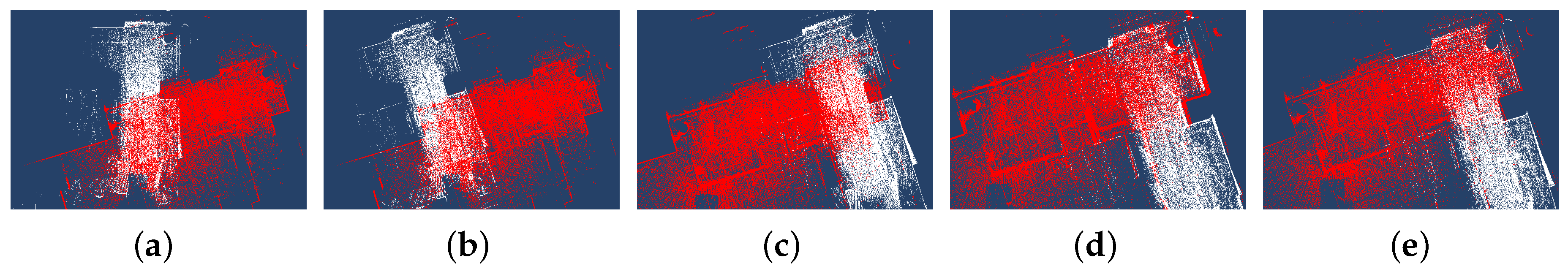
Algorithm 1 gives an outline of the proposed approach. Gaussian filter (lines 1–2) reduces the density of point-clouds so that the subsequent Sharp Features Detector (lines 3–4) provides less noisy extraction of points corresponding to sharp features. The output is filtered again by StatisticalOutlierFilter (which is part of the PCL library, see http://docs.point-clouds.org/1.7.1/classpcl_1_1_statistical_outlier_removal.html.) (lines 5–6) prior to a Line Detector (lines 7–8), which detects straight line features. The filtering steps are crucial in our outline as our method is sensitive to the output of the Line Detection algorithm (see Section 3.1). In the rest of the Algorithm 1, a search is performed to determine the optimal line features alignment. Possible alignment angles between and are found (line 10) by ignoring origins of lines in and and iteratively evaluating pair-wise cosine similarities for angle in small steps. Best candidates are then propagated for further calculation of the translational alignment over -plane. The search is performed on a surface of a geometric object fitted around point-cloud , where intersections of and with the surface are matched. This brings an advantage of effective match evaluation. The evaluation fitness function considers only positions of intersection points of lines and the objects surface. If an appropriate geometric object is chosen, we gain the advantage of the possibility of determining alignments over x and y axes one by one. That is, both the alignments are searched, avoiding a computationally expensive approach to perform search in a two-dimensional space. Both PossibleYTranslations and BestXTranslation use the aforementioned technique and are discused in Section 3.5.1 and Section 3.5.2 respectively. Refer to Figure 1 for illustration of the approach where given two unaligned point-clouds, the results for angle search, y-alignment, x-alignment and -refinement are plotted, respectively.
| Algorithm 1: Outline of our approach. |
 |
3.1. Line Detection
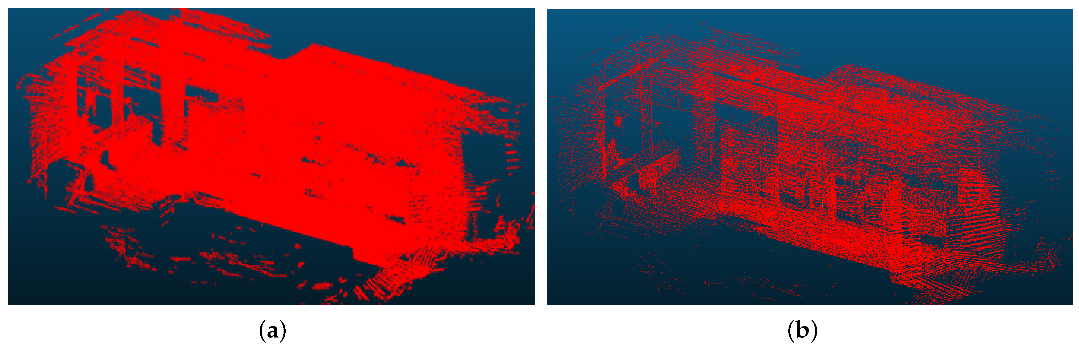
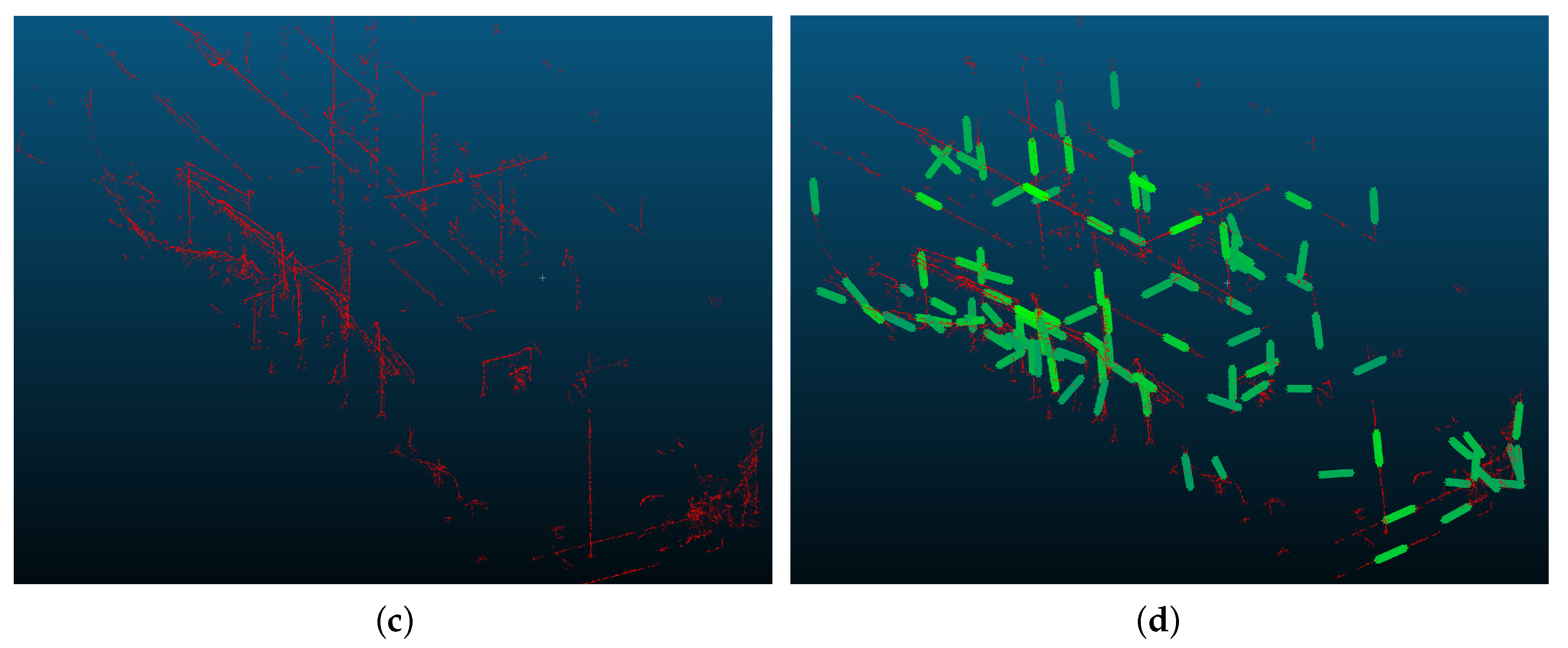
We use Hough Transform to find the sets and of the form where , are translation and direction vectors of a line m in point-cloud i respectively. In order to improve the accuracy and complexity of the method prior to line extraction, we extract subsets of both and which only contain points located on sharp features in the point-clouds (see the corresponding red points in Figure 2). This is because the line features of the point-cloud datasets are subsets of points lying on edges of arbitrary objects. Hence, points lying on smooth areas (e.g., in planar surfaces) can be omitted from the calculation.
3.1.1. Sharp Features Detection
An approach proposed by D. Bazazian, et al. [26] is used to detect points corresponding to sharp features, preceded by a convolution operation with a Gaussian kernel to improve the results. For each point , the surface variation as proposed by [27] is calculated as follows:
where are eigenvalues of the co-variance matrix of the point p k-neighborhood. All points with are considered to be subsets of smooth areas and are discarded from and , where denotes user-defined threshold and is obtained experimentally using the procedure given by authors in [26]. Finally, in order to lower noise in the output the StatisticalOutlierFilter is applied to discard points outside dense areas.
3.1.2. Line Features Detection
After the subsets and containing points corresponding to sharp features are identified, we proceed to find line features in them. We discretize the Hough parameter space by the method of [28] based on a tessellation of an icosahedron. This is followed by a modified version of Hough transform algorithm, which is applied iteratively and corrected by least squares error line fitting [28]. These two improvements results in greater accuracy. In order to avoid the exponential rise in the complexity in the subsequent steps, we limit the maximum number of line detection to 80 per scan. This number demonstrated to be sufficiently large for all of our experimental datasets.
3.2. Transformation Search
Once and are obtained an affine transformation is determined, such that best matches with . It can be decomposed as
Transformation matrix translates a point-cloud by a specified amount over the -plane, while rotates the point-cloud around the z-axis. The strength of our method lies in searching for the parameters x, y, , one by one, instead of considering their span as a search space. This results in a significant reduction in computational complexity.
We do not propose a global evaluation of which remains an interesting question for future research. Instead, in our step by step method where parameters x, y, are searched one by one, each parameter is rated according to its own fitness function, considering the parameters found in the previous steps as well. A small set of best rated possible values is then propagated to the next step to prune the search space of the parameters to be determined next. The fitness functions , , corresponding to the three parameters are defined in the following sections.
3.3. Determining Rotation between Point-Clouds
A rotation around the z-axis is found prior to searching for translation parameters. In our work, we do not consider rotations around other axes, which is sufficient in most, if not all, situations, as all LiDAR sensors determine the vector by the built-in gyroscope and orientate the point-cloud gravity downwards. We relax the problem by ignoring the origins of lines in and and find such that the nearest-neighborhood pair-wise cosine similarities between vectors of and are minimized, where is a 3D rotational matrix around z-axis. More specifically, assuming that direction vectors and are normalized, we define a fitness function as shown in Equation (2).
where × denotes a Cartesian product. By making sufficiently small, this product of scaled and shifted Gaussian functions rewards for a matching pairs of vectors whilst not matching pairs have almost no influence on the fitness value. This property is desirable because most vectors from and do not overlap by definition of the problem and hence the ideal algorithm would ignore them. We iteratively find best approximations of and for each of the best candidates, we run the steps described in the following sections.
3.4. Constructing a New Search Space
Once an angle between point-clouds has been determined, we proceed to find translation over the -plane. In our solution, we omit the translation over the z-axis in order to keep the proposed solution simple and present the idea more clearly. We leave a more general solution considering the translation over the z-axis as an interesting future research problem. We believe that this does not limit the applicability of our work in many real-world cases, e.g., matching indoor spaces on the same building floor or matching outdoor environments with a ground present.
The proposed approach avoids searching in a 3D space and avoids exhaustive repetitive calculations involving origins and directions of vectors. The key idea is to construct a geometrical object around a point-cloud and use its surface as a 2D transformed search space, where points correspond to intersections of vectors with this geometrical object.
3.4.1. Object Shape Selection
There are many choices for an object to be wrapped around a point-cloud. A naive solution is to use a plane (e.g., -plane underneath ). This choice involves a serious problem. Suppose there are two detected line features, one in point-cloud , another in such that their angles with the plane and are relatively small. Moreover, suppose they are sufficiently close to each other, i.e., , but . Hence we want our algorithm to recognize them as a potential match. However, even though , since the distance between the corresponding intersection points of the lines and the plane can get very large. Therefore, these two lines might be ignored by our algorithm despite the fact that they are very close to each other. Furthermore, as an angle of an arbitrary line with the plane tends to zero, the corresponding intersection point on the plane would tend to complex infinity and make the bounds of the search space extremely large. As a result, in practice many lines would need to be omitted from calculation resulting in a poor accuracy. The ideal solution for us seems to use a sphere constructed around , which completely solves this problem. However, as argued in Section 3.4.1, this makes the problem too complex to solve at this stage. We leave it as another possible extension of our work and focus on a simpler solution, that only partially solves the aforementioned problem, yet provides good results.
3.4.2. Fitting a Parabolic Cylinder
In case a parabolic cylinder is used as the shape of the wrapping object, only the lines with direction vectors parallel to the axis of the parabolic cylinder (i.e., the line ) are discarded from computation. For example, suppose we construct a parabolic cylinder with Equation (3).
where constants K and H are chosen such that all vectors of are guaranteed to intersect unless they are parallel to it. This is further discussed in Appendix A.2. For each we can hence find a constant t such that
See Appendix A.1 for more details about the solution to (4). Suppose are two such solutions. By Appendix A.2, either at least one of the solutions is real and left hand side of Equation (4) gives a point of intersection with or both the solutions tend to infinity. Hence vectors with for some threshold T are discarded from the following computations. Moreover, lowering T ignores position vectors of with a long distance to their points of intersections with in the directions of their direction vectors and, hence, lowers the noise in the output of the Line Detection stage for the future stages of calculation.
We can minimize the number of discarded vectors by rotating by angle around the z-axis. In order to simplify equations, suppose we rotate the point-clouds and by around the z-axis prior to the construction of to achieve the identical effect. Generally, most, if not all, of the possible values of should work unless we expect majority of line features to point in approximately the same direction. In this case, the value of can be set according to a domain-specific knowledge and we do not need to search for an optimal value of , which minimizes a number of omitted vectors as part of the algorithm. In our experiments, we found that ≥ vectors were preserved if we set to be an angle of with y-axis. Where and are eigenvectors of co-variance matrices and (Section 3.1) that correspond to largest eigenvalues found by Principal Component Analysis and T is a distance between two lines, i.e., intersections of and -plane. Here, we premised that many line features are either parallel or orthogonal to the scanning direction (e.g., wall edges, orientation of windows, etc.).
3.5. Translation Search Using Parabolic Cylinder Approach
Once a new search space has been constructed, we begin to find transformations over both the -axes on this space separately.
3.5.1. Finding First Translational Parameter
Algorithm 2 repeatedly calculates intersections of lines and a parabolic cylinder. It is, hence, essential that the implementation of these operations should be vectorized.
Suppose is a set of lines, where and stand for origin and direction vectors, respectively. Consider a parabolic cylinder representation from Equation (3). We propose the following linear time algorithm to find best candidates for alignment over the y-axis between corresponding point-clouds.
| Algorithm 2: Determining best translation over y-axis. |
 |
Details about used in the Algorithm 2 can be found in Appendix A.1. The algorithm uses fitness function (Equation (5)) which ignores dis-alignment on x-axis and uses arc length between nearest neighbors from and as a distance metric. Let,
where are y-coordinates of an intersection points on . We engineer in the manner similar to Equation (2).
The nearest neighbor function is implemented as a binary tree search and is discussed in Appendix B. is a distance between two lines of intersection of C and -plane. Scaling of by the distance between intersection point from the origin of a corresponding vector and C demonstrated to improve the accuracy of results, since this makes the sensitivity of score, i.e., the width of the Gaussian, takes into account the effect of amplification of inaccuracy, whose significance increases with the distance from line origins to their corresponding intersections (see Section 5.2 for details). The is a length of a shortest curve lying on projected onto -plane between points and . Hence it ignores the x-coordinates of the points and calculate the arc length assuming they share the same x-coordinate. Let be an equation of as in (3). Then the arc length can be expressed as
3.5.2. Determining Second Translational Parameter
Once the list of angles and translations over y-axis with highest fitness are determined, they are used to find the final remaining transformation over x-axis (see Algorithm 3). Just like in Algorithm 2, we determine the translation by an iterative search in small steps over all possible x-transformations and return an alignment with the highest fitness value.
| Algorithm 3: Determining best translations over x-axis. |
 |
The fitness function is a modified version of Equation (5). The modification lies in considering only difference in x-coordinates of nearest neighbors instead of the y-coordinate. One might argue that both the coordinates should be used for the determination of the final alignment. Although such an approach certainly improves accuracy, it complicates the nearest neighbor search. Our experiments show that we can still get sensible results by considering translations over both axes separately, i.e., finding them one by one instead of considering them as a pair while gaining a computational time speedup by using a binary search tree as discussed in Appendix B.
4. Experimental Evaluation
This section summarizes the coarse alignment search results and the post-ICP correction results. The experiments are conducted on the dataset generated at our research center, i.e., AIRC, AIST, Japan.
4.1. Dataset Description
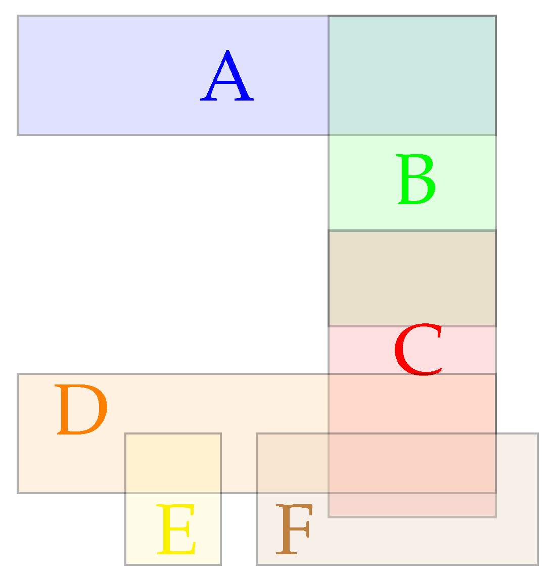
We acquired multiple point-cloud scans of the 8th floor of AIST, Tokyo Waterfront Area building using Kaarta Contour scanner, downsampled by the device with 0.5 cm resolution (The dataset used in the experiments can be downloaded from project repository https://github.com/Milos9304/LowOverlapPCRegistration.). The scanned environment imitates a typical household interior and the objects include various type of furniture, windows, sofa, television, bed, bathtub, etc. Overall, we perform six scans. Figure 3 shows the relative positions of each scans and Table 1 shows the overlapping ratios of the neighboring scans. Table 2 shows the corresponding sizes of each scan in number of points and in number of points after edge detection. The overlapping area of the neighboring scans is computed as follows:
4.2. Experimental Settings
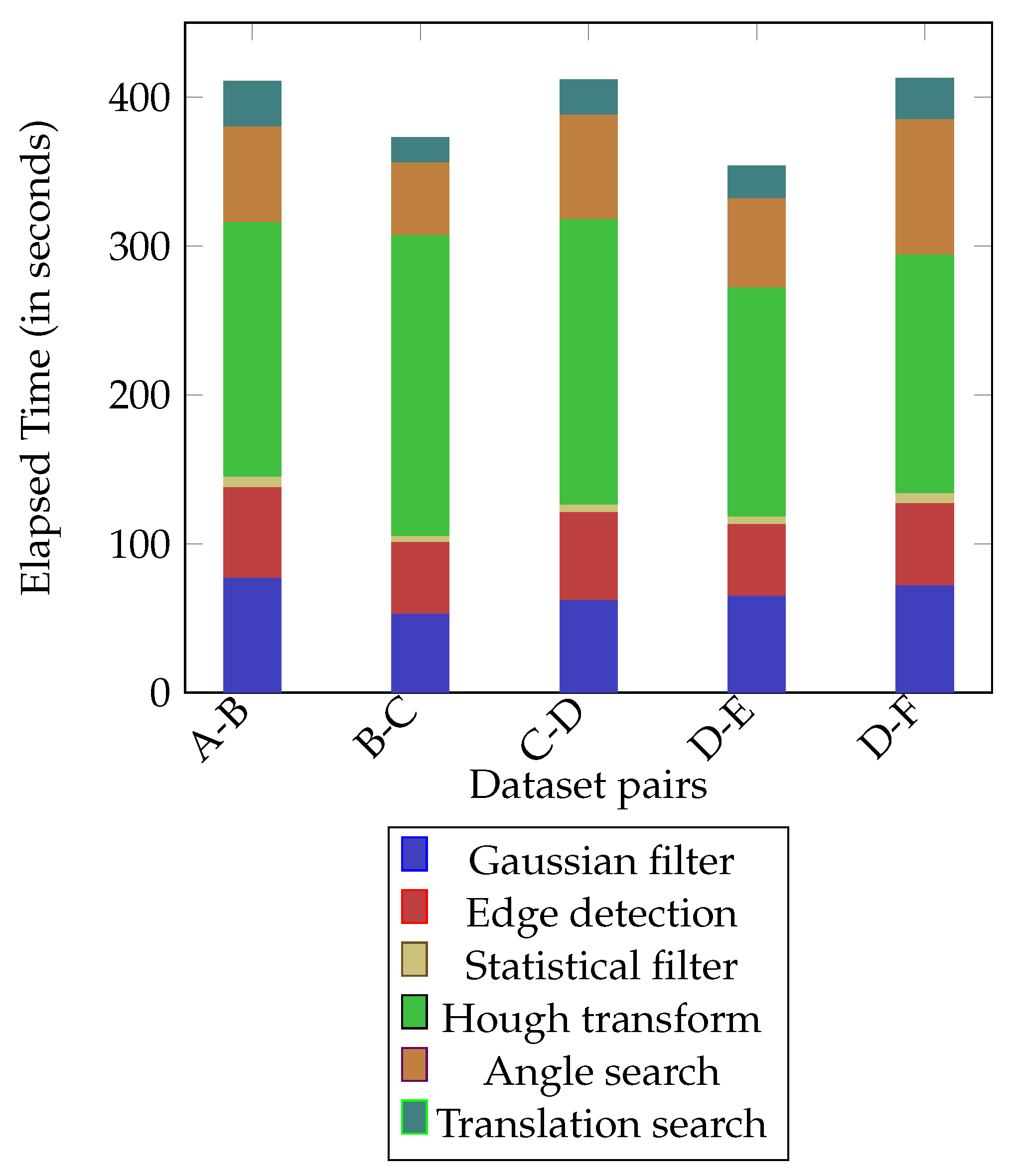
The experiments are performed on a Mac OS 10.13.6 machine with 3.3 GHz Intel Core i5 processor and 32 GB of RAM. We consider pairs of point-clouds from Table 1 and plot the runtime of each part of our algorithm in Figure 4. After a transformation is found and a merge is performed, we further run ICP algorithm just on the overlapping part to see if the results get improved. We discuss the results empirically and include the corresponding images in Figure 5. The left image shows the resulting alignment before ICP refinement and the right one after ICP refinement.
4.2.1. Parameter Tuning
Our approach requires many hyperparameters to be tuned in order to work correctly. We believe that the optimal setting is correlated with specification of input data like its density, noise, etc. The issue can be relaxed by using more aggressive preprocessing techniques like downsampling or upsampling to get desired densities and using various noise removal techniques [29]. In our experiments, we discovered that performing a Gaussian convolution filter with 3 cm radius improved the results of the subsequent Sharp Features detector with the parameter values experimentally computed and specified in [26]. The statistical outlier removal filter (which is part of the PCL library, see http://docs.point-clouds.org/1.7.1/classpcl_1_1_statistical_outlier_removal.html.) using 50-nearest neighbors with standard deviation multiplicator 0.05 is then applied to remove noise and outliers prior to running Hough Transform [28], which is a very important part of our outline. It must be tuned to achieve high precision and recall, otherwise, as discussed in Section 5, incorrect settings appear to deteriorate results significantly. Our experiments suggested to use different settings than the default ones with a step-width of 3 cm in -plane, minimum number of 300 votes per line and a maximum of 80 lines detected per scan, which avoids the exponential complexity in our approach. Moreover, in our experiments, it was sufficient to use the angle with the highest score and its 180-degrees rotated pair since the algorithm does not take the orientation of line features into account. The five best scored translations over the y-axis were propagated to the final stage, where corresponding x-translations were determined and the one with highest combined score has been chosen as the resulting alignment. The major difficulty turned out to be determining value in the fitness functions given by Equations (5) and (7), see Section 5.1 for details.
4.3. Experimental Results
The results, both before and after an ICP refinement are plotted in Figure 5 for each of the scan pairs of our dataset. Correspondingly, Table 3 summarizes the determined parameters of our approach and the ideal ones estimated by a manual alignment. It can be observed that our implementation worked for overlap ratios greater than 20%. For the smaller overlaps, one can observe that even though the resulting match was not accurate, the output was sensible. We believe that upon improving specific algorithms used in our outline, the approach would generalize over even lower overlapping ratios. See Section 5 for a general overview of discovered problems and their proposed solutions. Note that the optimal values of used in the fitness functions and had to be experimentally determined for each point-cloud pair separately (see Table 4). Hence, the current implementation of our work does not seem to generalize well over various different point-cloud pairs and futher improvements are required. See Section 5.1 for discussion about this issue and a proposed approach for the automatization of the process. Observe that the rotation search worked accurately in all the experiments. However, the accuracy of the search of translations over the y and x-axes is not satisfactory. The results can be summarized as follows:
- A–B and B–C: Our algorithm was capable of finding a close approximate alignment, which was corrected to a perfect fit after ICP refinement on the overlapping area.
- C–D: This pair is an example of failure of our algorithm to provide sufficiently good alignment, which could be corrected by ICP into a totally satisfactory result. Note, that even though the algorithm failed for the C-D pair, the result is still a reasonable approximation of the optimal transformation, suggesting further modifications can fix the issue.
- D–E: Both angle and translation over y-axis were calculated accurately. However, the final search for x-alignment failed. Exploring the dataset more closely, we found that similar line features occur periodically over the scan, which confuses the algorithm. Even though our approach is vulnerable to periodically occurring line features, an improved line detector algorithm can help to discard the false positive alignments.
- D–F: Another match that could be successfully refined by ICP into a correct alignment has been found. However, observe a large misalignment over y-axis prior to ICP correction which confirms that further modifications need to done. Also note that the value which resulted in correct match in this case is the same used for pairs A–B and B–C and resulted in accurate results (Table 4), suggesting that it is possible to improve our method to infer it automatically, as discussed in Section 5.1.
5. Discussion
In this section we discuss the shortcomings of our approach and their possible solutions. We are of the opinion that upon solving these individual problems the algorithm can be generalized for different types of data and provide reliable results such as in cases a) and b) of Figure 5.
5.1. Determining the Parameter
As pointed out in Section 4.2.1 the value of has a significant influence on the accuracy of the result. Assuming an ideal result of a line detector in both scans and , the value of can be theoretically set as close to zero as possible and hence, providing larger accuracy and reliability by successfully ignoring all the false line matches. By ideal result of a line detector, we mean extraction of all significant line features in scans with no inaccuracy in line position and direction. However, since the ideal result is very unlikely to be achieved, the value of should be large enough to accommodate the inaccuracies between positive matching pairs of lines, but at the same time small enough to ignore most of the false matches. Hence, we believe that a highly accurate line detector algorithm is an essential step to reduce the problem of determination of the parameter and, hence, generalize over wider variety of data. Moreover, as demonstrated in Equations (5) and (7) we used dynamic adjustment for each of the line pair by taking into account the distance from origins of the lines to their intersections on the quadratic surface constructed around . This is a naive approach that we did not test extensively, but we empirically observed improvements in our results. As discussed earlier, right value of has a crucial impact on the algorithm and, hence, this adjustment requires more serious attention.
5.2. Determining the Shape of the Geometrical Object Wrapped around
This work proposes to construct a geometrical object and then search for a transformation that best matches intersections of detected lines in scans and with the object. This significantly improves efficiency as evaluation of pair-wise matches given by a Cartesian product (Equation (1)) is not generally required and it should be sufficient to consider only its nearest neighbor on the 2D surface of the object. This can be found more efficiently using a binary search tree (see Appendix B). Our first try was to consider a plane as an object , but in the experiments, we found that the number of lines that had to be filtered out, i.e., those which were approximately parallel to the plane, was too large and resulting in poor results. Moreover, the issue of inaccuracy demonstrated to be amplified seriously in this case, i.e., a small difference in the line angle determined by line detection algorithm results in a large distance between corresponding intersection points if the lines are not approximately orthogonal to the plane.
Hence, the object should ideally wrap the point-clouds closely from each side (e.g., ideally a sphere), but should also allow efficient calculation of intersection points as in Appendix A.1. Furthermore, the object should enable the pruning of the search space by allowing to fix a translation over one particular axis, and once it has been found to proceed to the second one. This issue turned out to be complicated to overcome using a sphere due to complexity of mathematical formulas, although certainly not impossible. Using a parabolic cylinder we found a sufficient compromise that is easy to express mathematically despite its drawback that the lines parallel to it must be discarded from computation, although this is not so problematic to the extent as when a plane is being used.
We believe that the choice of a right shape not only minimizes the number of lines that need to be discarded but also most likely affects the way the value of (see Section 5.1) needs to be calculated, hence a wise choice of the object is another aspect of the work to be explored in more details.
5.3. Determining the Parameters of the Geometrical Object Wrapped around
As already pointed out, discarding lines due to not having an intersection point with the object O deteriorates the results and should be avoided. Hence the size of O needs to be large enough to minimize this effect, but at the same time small enough to minimize the aforementioned problem of inaccuracy amplification. See Appendix A.2 for our solution to this issue in case a parabolic cylinder is used.
Finding the ideal orientation of O seems to be more problematic. In addition to the constraints mentioned above, it is desirable that O is oriented in a way that the search ranges over both the y-axis and x-axis are approximately equal. If this is not the case, a search over a short range is less sensitive than the search over the larger one and these subsequent searches do not appear to fit well with each other during our experiments. We use a naive approach using Principal Component Analysis, in which we find eigenvectors of covariance matrices of the scans and . When projected on the -plane, we orientate the parabolic cylinder in a way that it is parallel to sum of the projected eigenvectors with the least eigenvalues. This method is also expected to minimize the number of discarded vectors in scans if they are parallel or orthogonal to the scanning direction. However, this assumption might not generalize well and we believe that more sophisticated methods are needed to improve the approach.
6. Conclusions and Future Work
This work introduces a novel method for point-cloud data registration with small overlapping regions. It suggests a different approach rather than modifying existing methods on matching detected keypoints by the ICP algorithm. Although such methods have demonstrated to work well with almost totally overlapping scans, they are not effective in case of the problem of low overlapping scans. The key concept adopted by this work is to reduce the representation of scans by detecting line features in them and to perform a search to match the largest number of lines. In order to prune a large transformation parameter space, the parameters are found one by one with the resultant fitness being a combination of fitness functions of its individual parameters. A quadratic surface fitting around the scans is suggested as a new search space for the parameters, where feature coordinates correspond to the intersections of lines and the surface. This achieves an effective evaluation of the pairwise matches between detected lines. The results suggest the rationality of our approach, as correct transformations amongst a subset of our dataset pairs were approximately determined. Running a subsequent ICP algorithm to refine them could find the exact optimal alignments down to a 20% overlapping area ratio and to the best of our knowledge, this is the least overlapping ratio for which a point-cloud registration technique has demonstrated to work. An interesting feature of the algorithm is that it has a bounded computational time of transformation search, provided that we bound the number of features detected in the scans. This is a reasonable relaxation if we can guarantee that they are evenly distributed over the scans. Hence, if such an efficient feature detector is designed, the approach scales with the same rate as the feature detector. Moreover, the method is very straightforward, i.e., it consists of subsequent steps independent of each other and, hence, it is easy to improve as modifying any of its components are expected to result in an overall increase in accuracy and/or performance. Therefore, we believe that despite the current instability of the approach, improving its individual components has a great potential to produce a fast, simple and reliable approach for partially overlapping point-cloud registration.
Our work can be extended by addressing its shortcomings discussed in detail in the discussion section. Our approach relies strongly on the preprocessing steps and the line detection algorithm. These steps not only influence accuracy of results of our proposed method of transformation search, but also make up to 75% of algorithm runtime, suggesting that using a more sophisticated method for line detection in terms of both speed and accuracy is a key step to make our method effective and applicable in real-world settings even without further ICP refinement. Secondly, our approach requires a large number of hyperparameters which must be tuned to get accurate results across different input pairs. This forced us to use different sensitivity values () in fitness functions for each dataset pair, hence, losing the generalization. Hence, the detection of parameter () is another important and interesting future research direction.
Author Contributions
Conceptualization, M.P., S.A.S. and K.-S.K.; methodology, M.P. and S.A.S.; software, M.P.; validation, M.P. and S.A.S.; formal analysis, M.P.; investigation, M.P. and S.A.S.; resources, M.P. and S.A.S.; data curation, M.P.; writing—original draft preparation, M.P. and S.A.S.; writing—review and editing, M.P. and S.A.S.; visualization, M.P.; supervision, S.A.S. and K.-S.K.; project administration, S.A.S. and K.-S.K.; funding acquisition, K.-S.K. All authors have read and agreed to the published version of the manuscript.
Funding
This work is partially supported by the project commissioned by the New Energy and Industrial Technology Development Organization (NEDO).
Conflicts of Interest
The authors declare no conflict of interest.
Appendix A. Parabolic Cylinder
Let
be an equation of a parabolic cylinder in a three dimensional space, where . In this appendix we propose a way to find its parameters K and H and derive an equation used in Algorithms 2 and 3 under its name , which calculates coefficients useful for fast determination of intersection points of lines and the parabolic cylinder in a program loop cycle.
Appendix A.1. Finding Intersection of Lines and Parabolic Cylinder
Suppose is set of lines for which we are interested to find points of intersection with and let
with being position vector of s and its direction vector. As depicted in (Algorithm 2), we keep increasing by small steps in a loop cycle and hence we are interesting to express the formula for t in terms of , where with being the original alignment of s without any shift along y-axis. s has an intersection with of the form
if and only if
Solving for t we derive a quadratic equation
which can be simplified into a form
where
Since calculation of does not involve parameter , they can be calculated prior to executing a loop cycle, where only (A2) gets evaluated.
Appendix A.2. Determining Parameters of Parabolic Cylinder
When determining parameters H and K of parabolic cylinder , we should not aim for high parameters in order to minimize mean distance from origins of lines to their intersection points with so that the inaccuracies in line directions returned by LineDetector algorithm (Section 3.1) do not amplify significantly. At the same time no vector from a set of lines should be discarded from our outline due to having no intersection point with unless it is parallel to it, i.e., unless . The parabolic cylinder is being constructed around point-cloud , see (Algorithm 1). Since is static and only is shifted during our algorithm, when determining an intersection of with it is sufficient to set and evaluate
hence
Suppose without loss of generality, that . If this is not the case, just multiply direction vector of a by getting a modified expression of the same line. Hence is a sufficient condition for a to have an itersection with , or more generally, letting
ensures all vectors of have common solution with unless they are parallel to it and discarded from computational baseline. Accordingly, may be arbitrary in ideal case, where no inaccuracies are propagated in the computation. However, finding an optimal value of K helps to leverage the aforementioned problem of amplifying inaccuracies. In our experiments the best value that seemed to work reasonably well was setting it such that the distance between intersection lines of and -plane was approximately similar to length of bounding box of (see Algorithm 1) in y-axis direction . Following this reasoning, let in and in Equation (3) to achieve the desired setting. In this case, the value of K is obtained as
| Algorithm A1: Construction of binary search tree used in our implementation. |
 |
Appendix B. Binary Nearest Neighbor Search
This appendix section discusses details about functions and used in fitness functions (5) and (7) with the purpose of finding nearest neighboring intersection point on in y and x directions respectively. Because of their usage in loop cycles, their implementation is critical for the overall speed of the algorithm. For the sake of discussion, let denote any of y or x direction. In addition to returning a nearest neighbor, also its direction from corresponding line origin is returned and used as a scaling factor of standard deviation (see Equations (5) and (7)) to tackle the issue of inaccuracy amplification. The construction of the binary search tree (see Algorithm A1) is rather a standard one, with a minor modification, that a condition at the root node selects between two halves of the quadratic cylinder bisected by a line passing through all the points with the highest coordinates in z-axis (i.e., on the top of it in a parallel direction) to distinguish what side of the cylinder is used for neighborhood search.
References
- Fraeman, A.A.; Castillo-Rogez, J.C.; Wyatt, E.J.; Chien, S.A.; Herzig, S.J.; Gao, J.L.; Troesch, M.; Vaquero, T.S.; Walsh, W.B.; Belov, K.V.; et al. Assessing Martian Cave Exploration for the Next Decadal Survey; Mars Exploration Program Analysis Group (MEPAG): Washington, DC, USA, 2018. [Google Scholar]
- Troesch, M.; Vaquero, T.; Byon, A.; Chien, S. A Journey Through an Autonomous Multi-rover Coordination Scenario in Mars Cave Exploration. In Proceedings of the International Conference on Planning and Scheduling (ICAPS 2018) System Demonstrations and Exhibits Track, Delft, The Netherlands, 24–29 June 2018. [Google Scholar]
- Hörner, J. Automatic Point Clouds Merging. Master’s Thesis, Charles University, Faculty of Mathematics and Physics, Prague, Czech Republic, 2018. [Google Scholar]
- Pomerleau, F.; Colas, F.; Siegwart, R. A Review of Point Cloud Registration Algorithms for Mobile Robotics. NOW 2015, 4, 1–104. [Google Scholar] [CrossRef] [Green Version]
- Meng, J.; Li, J.; Gao, X. An accelerated ICP registration algorithm for 3D point cloud data. Proc. SPIE 2019, 10839. [Google Scholar] [CrossRef]
- Kamencay, P.; Sinko, M.; Hudec, R.; Benco, M.; Radil, R. Improved Feature Point Algorithm for 3D Point Cloud Registration. In Proceedings of the 2019 42nd International Conference on Telecommunications and Signal Processing (TSP), Budapest, Hungary, 1–3 July 2019; pp. 517–520. [Google Scholar] [CrossRef]
- Prakhya, S.M.; Liu, B.; Lin, W. Detecting keypoint sets on 3D point clouds via Histogram of Normal Orientations. Pattern Recognit. Lett. 2016, 83, 42–48. [Google Scholar] [CrossRef]
- Li, J.; Lee, G.H. USIP: Unsupervised Stable Interest Point Detection from 3D Point Clouds. arXiv 2019, arXiv:1904.00229. [Google Scholar]
- Tonioni, A.; Salti, S.; Tombari, F.; Spezialetti, R.; Stefano, L.D. Learning to Detect Good 3D Keypoints. Int. J. Comput. Vis. 2018, 126, 1–20. [Google Scholar] [CrossRef]
- Prakhya, S.; Lin, J.; Chandrasekhar, V.; Lin, W.; Liu, B. 3DHoPD: A Fast Low Dimensional 3D Descriptor. IEEE Robot. Autom. Lett. 2017, 2, 1472–1479. [Google Scholar] [CrossRef]
- Seo, J.H.; Kwon, D.S. Learning 3D local surface descriptor for point cloud images of objects in the real-world. Robot. Auton. Syst. 2019, 116, 64–79. [Google Scholar] [CrossRef]
- Prakhya, S.M.; Liu, B.; Lin, W. B-SHOT: A binary feature descriptor for fast and efficient keypoint matching on 3D point clouds. In Proceedings of the IEEE/RSJ International Conference on Intelligent Robots and Systems (IROS), Hamburg, Germany, 28 September–2 October 2015; pp. 1929–1934. [Google Scholar]
- Sharp, G.C.; Lee, S.W.; Wehe, D.K. ICP registration using invariant features. IEEE Trans. Pattern Anal. Mach. Intell. 2002, 24, 90–102. [Google Scholar] [CrossRef] [Green Version]
- He, Y.; Liang, B.; Yang, J.; Li, S.; He, J. An Iterative Closest Points Algorithm for Registration of 3D Laser Scanner Point Clouds with Geometric Features. Sensors 2017, 17, 1862. [Google Scholar] [CrossRef] [PubMed] [Green Version]
- Salvi, J.; Matabosch, C.; Fofi, D.; Forest, J. A review of recent range image registration methods with accuracy evaluation. Image Vis. Comput. 2007, 25, 578–596. [Google Scholar] [CrossRef] [Green Version]
- Makadia, A.; Patterson, A.; Daniilidis, K. Fully Automatic Registration of 3D Point Clouds. In Proceedings of the 2006 IEEE Computer Society Conference on Computer Vision and Pattern Recognition (CVPR’06), New York, NY, USA, 17–22 June 2006; Volume 1, pp. 1297–1304. [Google Scholar] [CrossRef] [Green Version]
- Horn, B.K.P. Extended Gaussian images. Proc. IEEE J. 1984, 72, 1671–1686. [Google Scholar] [CrossRef]
- Yang, J.; Li, H.; Campbell, D.; Jia, Y. Go-ICP: A Globally Optimal Solution to 3D ICP Point-Set Registration. arXiv 2016, arXiv:1605.03344. [Google Scholar] [CrossRef] [PubMed] [Green Version]
- Stechschulte, J.; Ahmed, N.; Heckman, C. Robust low-overlap 3-D point cloud registration for outlier rejection. In Proceedings of the 2019 International Conference on Robotics and Automation (ICRA), Montreal, QC, Canada, 20–24 May 2019; pp. 7143–7149. [Google Scholar] [CrossRef]
- Mellado, N.; Mitra, N.; Aiger, D. Super 4PCS Fast Global Pointcloud Registration via Smart Indexing. Comput. Graph. Forum 2014, 33. [Google Scholar] [CrossRef] [Green Version]
- Torres, D.; Cuevas, F. Three-dimensional Point-cloud Registration using a Genetic Algorithm and the Iterative Closest Point Algorithm. In Proceedings of the International Conference on Evolutionary Computation Theory and Applications (FEC-2011), Paris, France; 24–26 October 2011; pp. 547–552. [Google Scholar]
- Zhang, X.; Yang, B.; Li, Y.; Zuo, C.; Wang, X.; Zhang, W. A method of partially overlapping point clouds registration based on differential evolution algorithm. PLoS ONE 2018, 13, e0209227. [Google Scholar] [CrossRef] [PubMed] [Green Version]
- Silva, L.; Bellon, O.R.P.; Boyer, K.L. Precision Range Image Registration Using a Robust Surface Interpenetration Measure and Enhanced Genetic Algorithms. IEEE Trans. Pattern Anal. Mach. Intell. 2005, 27, 762–776. [Google Scholar] [CrossRef] [PubMed]
- Theiler, P.; Schindler, K. Automatic registration of terrestrial laser scanner point clouds using natural planar surfaces. ISPRS Ann. Photogramm. Remote Sens. Spat. Inf. Sci. 2012, 3, 173–178. [Google Scholar] [CrossRef] [Green Version]
- Eckart, B.; Kim, K.; Kautz, J. EOE: Expected Overlap Estimation over Unstructured Point Cloud Data. In Proceedings of the 2018 International Conference on 3D Vision (3DV), Verona, Italy, 5–8 September 2018; pp. 747–755. [Google Scholar] [CrossRef] [Green Version]
- Bazazian, D.; Casas, J.R.; Ruiz-Hidalgo, J. Fast and Robust Edge Extraction in Unorganized Point Clouds. In Proceedings of the 2015 International Conference on Digital Image Computing: Techniques and Applications (DICTA), Adelaide, SA, Australia, 23–25 November 2015; pp. 1–8. [Google Scholar] [CrossRef] [Green Version]
- Pauly, M.; Gross, M.; Kobbelt, L.P. Efficient simplification of point-sampled surfaces. In Proceedings of the IEEE Visualization (VIS 2002), Boston, MA, USA, 27 October–1 November 2002; pp. 163–170. [Google Scholar] [CrossRef] [Green Version]
- Dalitz, C.; Schramke, T.; Jeltsch, M. Iterative Hough Transform for Line Detection in 3D Point Clouds. Image Process. Line 2017, 7, 184–196. [Google Scholar] [CrossRef] [Green Version]
- Han, X.F.; Jin, J.; Wang, M.J.; Jiang, W.; Gao, L.; Xiao, L. A review of algorithms for filtering the 3D point cloud. Signal Process. Image Commun. 2017, 57. [Google Scholar] [CrossRef]
Figure 1.
Step by step outline of the low overlapping point-cloud registration. (a) original alignment (b) result of rotation search (c) result of translation over y axis (d) result of translation over x axis (e) Iterative Closest Point (ICP) refinement
Figure 1.
Step by step outline of the low overlapping point-cloud registration. (a) original alignment (b) result of rotation search (c) result of translation over y axis (d) result of translation over x axis (e) Iterative Closest Point (ICP) refinement

Figure 2.
Outline of line detection: (a) Original point-cloud scan, (b) Point-cloud after convolution with Gaussian kernel, (c) Result of sharp features extraction and subsequent filteration by StatisticalOutlierFilter, (d) Line detection after edge detection phase. A green unit length marker indicates the corresponding line has been detected. Note that it does not depict any information about line length which is ignored in our approach.


Figure 3.
Relative positions of dataset scans.

Figure 4.
Runtime analysis.

Figure 5.
Results on the dataset pairs. Left image shows resulting alignment before ICP refinement and the right one after ICP refinement. Pairs: (a) A-B, (b) B-C, (c) C-D, (d) D-E, (e) D-F.
Figure 5.
Results on the dataset pairs. Left image shows resulting alignment before ICP refinement and the right one after ICP refinement. Pairs: (a) A-B, (b) B-C, (c) C-D, (d) D-E, (e) D-F.


Table 1.
Overlapping ratios of dataset scans.
| Pair | Overlap Ratio |
|---|---|
| A-B | 20.25% |
| B-C | 29.36% |
| C-D | 16.54% |
| D-E | 15.22% |
| D-F | 26.73% |
Table 2.
Size of point-clouds.
| ID | # Points | # Points after Edge Detection |
|---|---|---|
| A | 2,715,304 | 351,036 |
| B | 1,350,946 | 124,001 |
| D | 1,900,559 | 194,050 |
| E | 1,213,707 | 153,252 |
| F | 1,449,478 | 222,750 |
Table 3.
Parameters obtained by our approach before ICP refinement. Significant errors are colored in red. Angles are in radians and translation distances are in meters.
Table 3.
Parameters obtained by our approach before ICP refinement. Significant errors are colored in red. Angles are in radians and translation distances are in meters.
| Calculated | Target | |||||
|---|---|---|---|---|---|---|
| Angle | Angle | |||||
| A-B | 0.31134 | −1.858 | −7.347 | 0.31121 | −1.818 | −7.496 |
| B-C | 3.10700 | 1.761 | −0.698 | 3.10698 | 3.531 | −0.438 |
| C-D | 1.67724 | 2.840 | −2.308 | 1.67842 | 3.528 | −3.140 |
| D-E | 3.81791 | 0.340 | −1.963 | 3.81785 | 0.824 | −1.890 |
| D-F | 5.3178 | 3.901 | −4.450 | 5.3166 | 3.892 | −4.191 |
Table 4.
Sigma values used in our experiments
| A-B | B-C | C-D | D-E | D-F | |
|---|---|---|---|---|---|
© 2019 by the authors. Licensee MDPI, Basel, Switzerland. This article is an open access article distributed under the terms and conditions of the Creative Commons Attribution (CC BY) license (http://creativecommons.org/licenses/by/4.0/).
Share and Cite
MDPI and ACS Style
Prokop, M.; Shaikh, S.A.; Kim, K.-S. Low Overlapping Point Cloud Registration Using Line Features Detection. Remote Sens. 2020, 12, 61. https://0-doi-org.brum.beds.ac.uk/10.3390/rs12010061
AMA Style
Prokop M, Shaikh SA, Kim K-S. Low Overlapping Point Cloud Registration Using Line Features Detection. Remote Sensing. 2020; 12(1):61. https://0-doi-org.brum.beds.ac.uk/10.3390/rs12010061
Chicago/Turabian StyleProkop, Miloš, Salman Ahmed Shaikh, and Kyoung-Sook Kim. 2020. "Low Overlapping Point Cloud Registration Using Line Features Detection" Remote Sensing 12, no. 1: 61. https://0-doi-org.brum.beds.ac.uk/10.3390/rs12010061
Note that from the first issue of 2016, this journal uses article numbers instead of page numbers. See further details here.