Dimensionality Reduction and Feature Selection for Object-Based Land Cover Classification based on Sentinel-1 and Sentinel-2 Time Series Using Google Earth Engine

Abstract

Mapping Earth’s surface and its rapid changes with remotely sensed data is a crucial task to understand the impact of an increasingly urban world population on the environment. However, the impressive amount of available Earth observation data is only marginally exploited in common classifications. In this study, we use the computational power of Google Earth Engine and Google Cloud Platform to generate an oversized feature set in which we explore feature importance and analyze the influence of dimensionality reduction methods to object-based land cover classification with Support Vector Machines. We propose a methodology to extract the most relevant features and optimize an SVM classifier hyperparameters to achieve higher classification accuracy. The proposed approach is evaluated in two different urban study areas of Stockholm and Beijing. Despite different training set sizes in the two study sites, the averaged feature importance ranking showed similar results for the top-ranking features. In particular, Sentinel-2 NDVI, NDWI, and Sentinel-1 VV temporal means are the highest ranked features and the experiment results strongly indicated that the fusion of these features improved the separability between urban land cover and land use classes. Overall classification accuracies of 94% and 93% were achieved in Stockholm and Beijing study sites, respectively. The test demonstrated the viability of the methodology in a cloud-computing environment to incorporate dimensionality reduction as a key step in the land cover classification process, which we consider essential for the exploitation of the growing Earth observation big data. To encourage further research and development of reliable workflows, we share our datasets and publish the developed Google Earth Engine and Python scripts as free and open-source software.

1. Introduction

Mapping Earth’s surface and its rapid changes with remotely sensed data are a crucial task to help understand the impact of an increasingly urban world population on the environment. The information provided by urban scene classification and change maps are quite important for urban planners, environmental engineers, and decision makers in general. Land Use/Land Cover (LULC) classes are established categorical variables that represent the status of the Earth’s surface in a viable way. In the last couple decades, several studies have investigated the classification of urban scenes using remote sensing data. Remotely sensed data provides cheap, comprehensive, and easy to use source to map the location and the spatial extent of different LULC classes. With its rich information content, multispectral optical images have been used intensively for urban scene classification [1,2,3,4,5,6]. Unlike optical, radar images have lower spectral information content. Nevertheless, these images are not affected by atmospheric and solar illumination conditions. Several studies have shown the potential of these images in urban classification [7,8,9,10,11,12,13]. The successful use of remote sensing data for urban scene classification depends on several considerations (e.g., image spatial resolution, acquisition time, spectral information, classification scheme, etc.). Another factor of crucial importance and that has strong impact on the classification accuracy, in general, is the input features and their quality. It is quite common to use the raw input spectral images (e.g., green, red, NIR, radar cross section, etc.), or/and product derived from these spectral bands (e.g., NDBI, NDVI, NDWI) as input features. Texture measures (e.g., GLCM texture) have also played important role in increasing the discrimination between different LULC classes [14,15]. Features that can be used for scene classification are not restricted to raw image spectral bands or products derived from them. Several studies have shown that combining features extracted from images acquired at different times could help significantly improving the classification accuracy [11,16,17,18,19]. The basic idea is that despite the fact that some LULC classes would look very similar in one season/time, they tend to look quite different in another. By combining images acquired in different times, therefore, it is possible increase classes’ separability.

Because of their different modalities, optical and SAR provide quite different information about earth surface. The response of earth surface materials to the short wavelength energy used by optical sensors depends to a high extent on the biochemical properties of the observed objects. Conversely, radar response is often associated with other factors such as objects geometrical properties (e.g., roughness), and its moisture content. It is therefore natural to think of SAR and optical images as complementary to each other [20]. Several studies have investigated the possibility to improve classification accuracy through the fusion of SAR and optical images [21,22,23]. Fusion can be carried out at the feature, pixel, or information level. The former approach consists of combining features extracted from different data sources into a one augmented feature vector; it can then be an input of any classification algorithm. Because of the simplicity involved, this approach has been the focus of several studies [24,25,26,27,28]. In fact, the multitemporal image classification approach discussed in the previous section can be envisaged as a feature-level fusion technique; this approach was further extended by the fusion of multitemporal and multi-source features extracted from Radarsat-2 and QuickBird images for urban land-cover mapping [29]. Despite the availability of a large selection of features that can be used for the classification task, most studies only consider a few of them. This could be attributed to the fact that in many cases features will be highly correlated, i.e., they contain redundant information. Including such features would serve nothing other than slowing down the classification process. Another reason is that features computation (e.g., GLCM textures) is time consuming and handling large dataset with many features is not easy in common image classification software [30]. For this reason, the analyst faces the problem of selecting few out of hundredth of available features (e.g., spectral band, GLCM textures, and indices). Usually, expert knowledge is used to manually select a few, allegedly promising features, even though numerous algorithms exist that could perform the dimensionality reduction task automatically [31,32,33,34,35,36].

Dimensionality reduction is the process of simplifying the classification task by either transforming the original features to a representation in a set of lower dimensionality (feature extraction) or by removing redundant and irrelevant features (feature selection) [37]. A well-known feature extraction method is principal component analysis (PCA) [38]. It projects the input feature space to a new space in which feature will be uncorrelated. It also compresses (i.e., dimensionality reduction) the information into few output features that contain most of the information available in the original space. Unlike PCA, linear discriminant analysis (LDA) is a supervised feature extraction method that projects the input feature space in a way that maximizes the separation between the classes [39]. With large representative training data, LDA is expected to outperform PCA since it takes samples classes into consideration [40]. Feature selection methods can be grouped into three main categories: filters, wrappers, and embedded methods [37,41]. While filters rank features according to some predefined statistic and remove lowest ranking features, wrappers utilize learning machines to find the best performing subset of features. Embedded methods find optimal feature subsets during training and are integral parts of certain learning machines. In particular, filters are independent of the learning machine and they evaluate feature importance based on data characteristics [42]. Univariate filters compute a feature’s quality individually, assuming independence between the features, while multivariate filters take possible dependencies into account and perform assessment in batches.

The frequent acquisition of satellite imagery leads to an impressive amount of data that is collected and published on a daily basis. An efficient means of access and an infrastructure that allows large-scale processing of this big EO data are needed to fully exploit it. Google Earth Engine (GEE) is a cloud-based platform for planetary-scale geospatial analysis that utilizes the massive computational capabilities of Google’s servers. It facilitates access to geographical and remote sensing data in their “multi-petabyte analysis-ready data catalog” [43]. GEE allows for effective processing through subdivision and distribution of computations. In general, GEE lowers the threshold for large-scale geospatial computation and makes it possible “for everyone” [43]. Though, GEE offers valuable opportunities for EO data analysis it could be vastly enhanced with an integration with Google Cloud Platform (GCP) (https://cloud.google.com/). GCP provides Google Compute Engine, which offers scalable and customizable virtual machines for cloud computing and Google Cloud Storage, a service for storing and accessing data. It allows different types of storage based on the desired access-frequency and the intended use. On GCP, external libraries can be used for further processing and deeper analysis of data derived from GEE. One example is Scikit-learn, an open-source machine learning Python module [44]. It contains a variety of machine learning models for classification, regression, and clustering [45]. Besides implementations of machine learning models, it contains tools for model selection, cross-validation, hyperparameter tuning, and model evaluation as well as dimensionality reduction, feature decomposition, and feature selection.

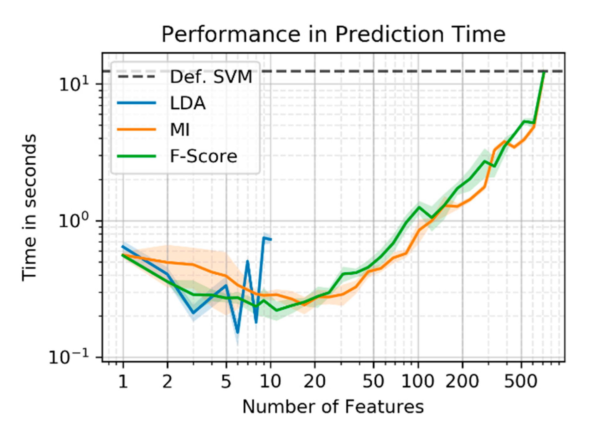
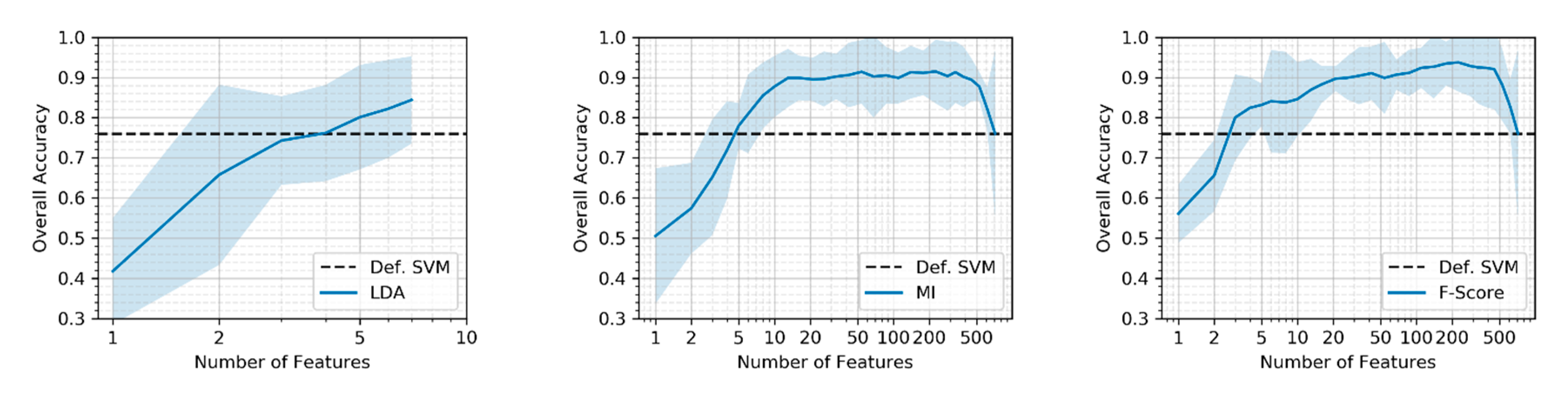
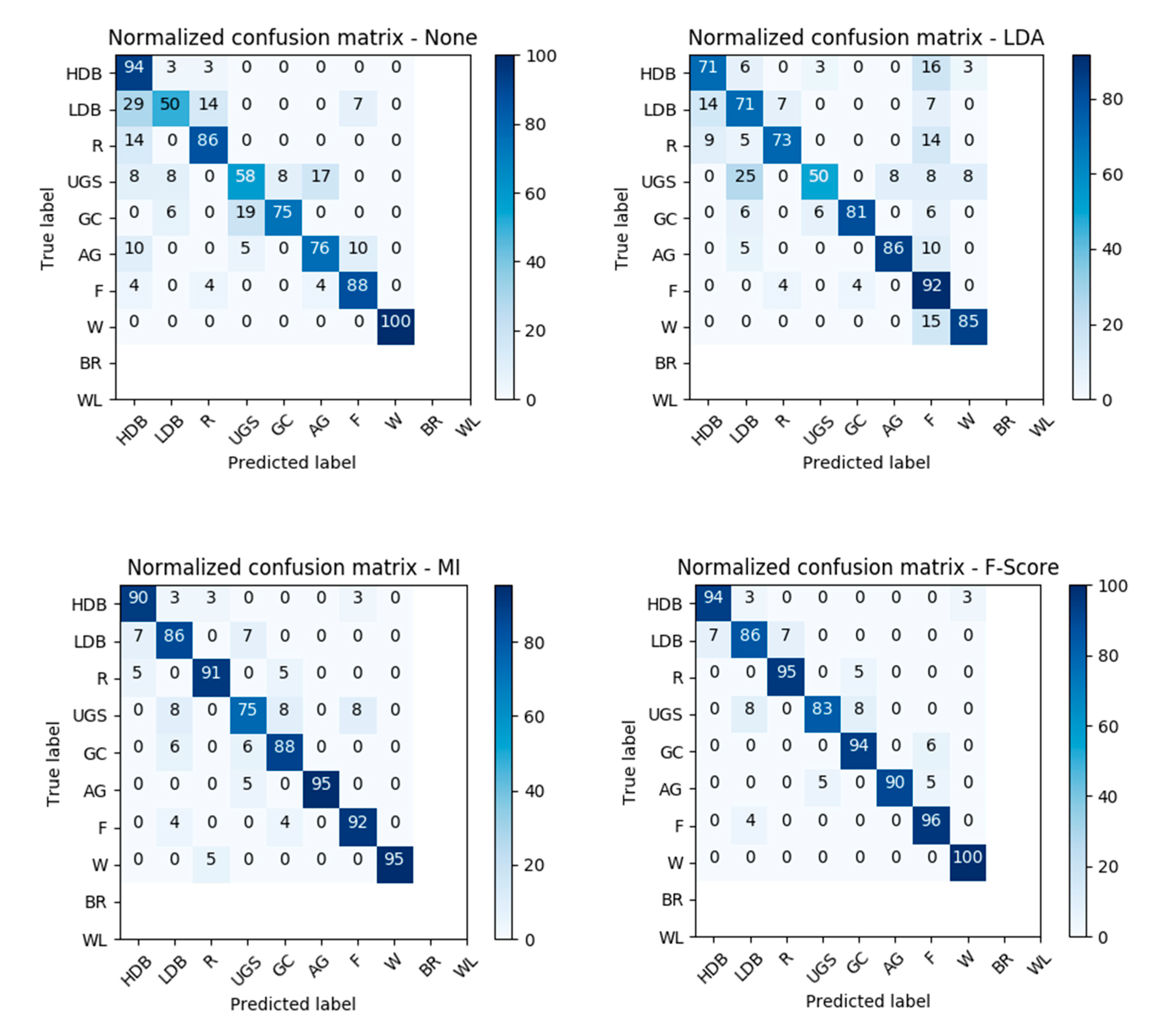
In this study, we will utilize the computational power of Google Earth Engine (GEE) and Google Cloud Platform (GCP) to generate an oversized feature set extracted form Sentinel1 and Sentinel2 multitemporal images. We will explore feature importance and analyze the potential of different dimensionality reduction methods. A large feature set is evaluated to find the most relevant features which discriminate the classes well and thereby contribute most to achieve high classification accuracy. In doing so, we present an automated alternative to the sensitive knowledge-based but tedious and sometimes biased selection of input features. Three methods of dimensionality reduction, i.e., linear discriminant analysis (LDA), mutual information-based (MI), and Fisher-criterion-based (F-Score), will be tested and evaluated. LDA is a feature extraction method that transform the original feature space into a projected space of lower dimensionality. MI and F-score belong to the group of filter-based univariate feature selection methods that rank and filter the features according to some statistic. We evaluate the optimized feature sets against an untreated feature set in terms of classification accuracy, training and prediction performance, data compression, and sensitivity to training set sizes.

For features classification, a support vector machine (SVM) is chosen. SVM is a supervised non-parametric machine learning algorithm [46]. Although it is commonly used for classification tasks, it has also been used for regression. SVM maps the input features space to a higher dimensional space using kernel functions (e.g., radial basis function). The training samples are separated in the new space by a hyperplane (defined by the support vectors) that guarantee the largest margin between the classes. It has been used successfully in different types of remote sensing applications—for example, classification [47,48,49], change detection [50,51,52], and in image fusion [53]. Depending on the size of the training sample, SVM is known for being slow during the training phase. However, the classification phase is quite fast since it only depends on a few training samples known as the support vector. The spatial resolutions of Sentinel-1 (S1) SAR data and Sentinel-2 (S2) MSI sensors are moderate (e.g., 10 m) and the classification will often use the pixel-based approach. Geographic object-based image analysis (GEOBIA) is often applied when using high spatial resolution data [54,55]. However, given the large extent of the study areas, which surpasses even the largest case studies compared in a recent review of object-based methods by a factor of a thousand [56], we adopted an object-based classification even though the analysis will be based on S1 and S2 images. The application of GEOBIA to moderate spatial resolution is not very common, however is not rare either [57]. The object-based paradigm allows us to reduce the computational complexity immensely, and consequently, allow us to put more emphasis on the main goal of this paper, which is the investigation of feature selection for urban scenes classification.

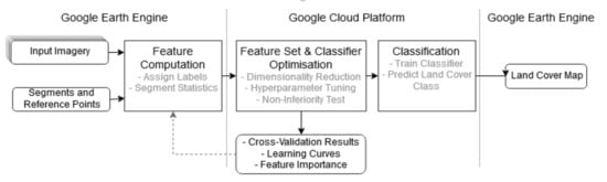
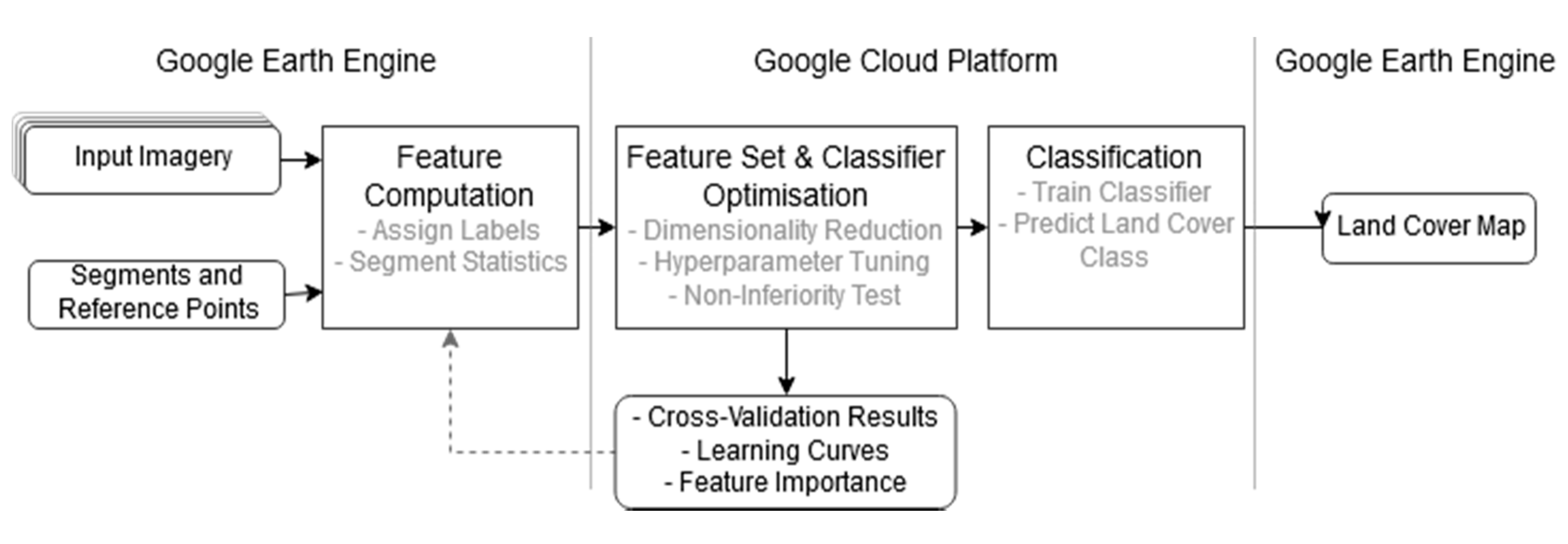
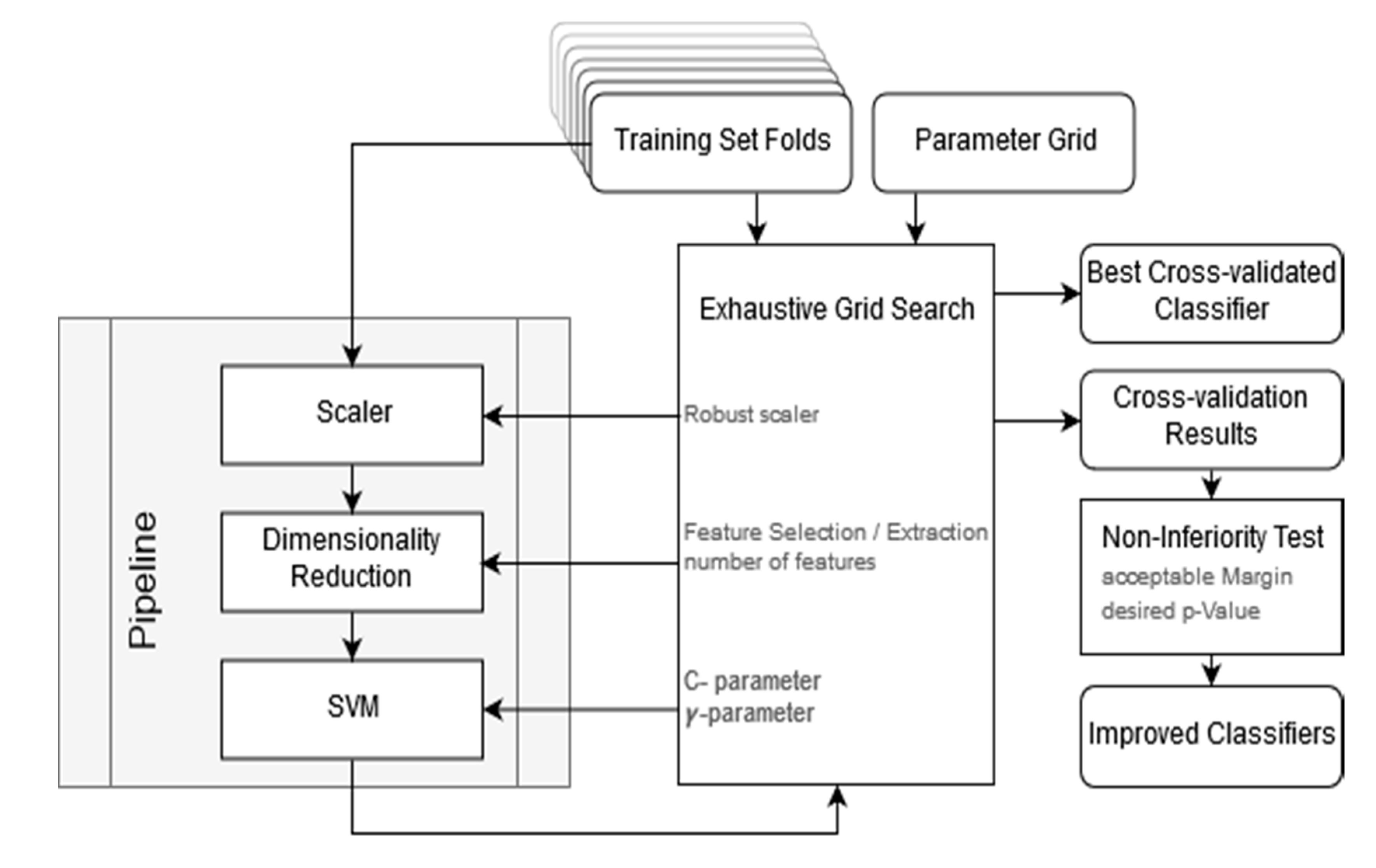
In summary, we provide a framework that derives features from GEE’s data catalogue. We deliver a prototype for GCP that applies dimensionality reduction and feature set optimization methods and tunes the classifier’s hyperparameters in an exhaustive search. Performances on the different feature sets are compared to each other with statistical measures, different visualization methods, and a non-inferiority test for the highest dimensionality reduction satisfying the chosen performance requirements. The overall aim is the exploration of feature importance in the big EO data that are available today. Understanding the feature importance leads to an improved classification accuracy by the removal of irrelevant features and to an increased classification throughput by the reduction of the datasets. We demonstrate the applicability of our methodology in two different study sites (i.e., Stockholm and Beijing) based on a multitemporal stack of S1 and S2 imagery. For the given classification scheme, we find the best feature set that achieve the highest overall accuracy. A further analysis of the feature selection allows us to evaluate the importance of individual features to the classification task.

2. Study Areas and Data Description

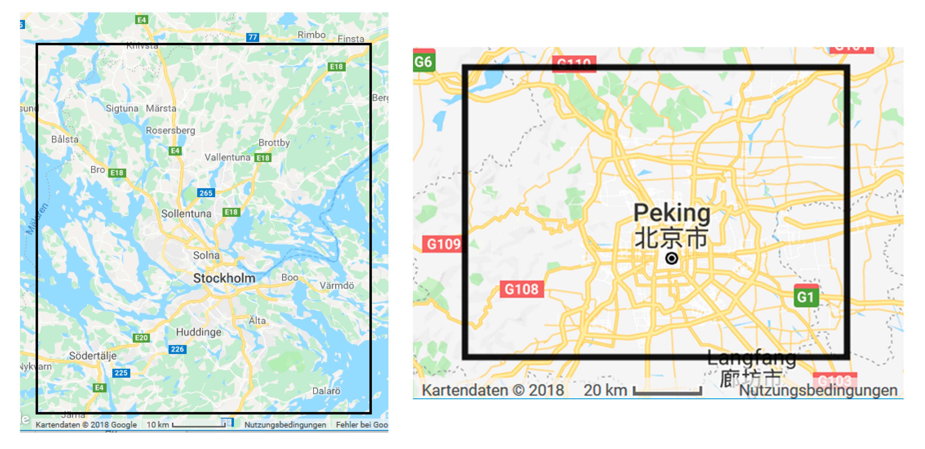
We demonstrate our methodology on two study areas. One is based on a scheme of 10 LULC classes in the urban area of Stockholm, while the other is based on 8 LULC classes scheme in the urban area of Beijing. The study areas are shown in (Figure 1) and cover 450,000 ha in Stockholm and 518,000 ha in Beijing. The classes represent the dominant land cover and land use types in the respective areas as demonstrated in [58,59], and are derived from urban planning applications and urban sprawl monitoring. The classification schemas adopted for the study areas were defined in previous projects [58,59] to monitor the urbanization process and evaluate the corresponding environmental impact;

Table 1. Classification schema in Stockholm and Beijing.

Class	Description	Stockholm		Beijing
		No. Reference Points	No. Sample Segments	No. Reference Points	No. Sample Segments
1-HDB	High-density built-up	1000	986	150	134
2-LDB	Low-density built-up	1000	926	150	54
3-R	Roads and Railroads	1009	166	153	89
4-UGS	Urban green spaces	1045	571	70	63
5-GC	Golf courses	1013	275	80	73
6-AG	Agriculture	1045	866	160	133
7-F	Forests	1000	908	218	175
8-W	Water	1000	780	161	93
9-BR	Bare rock	503	172	None	None
10-WL	Wetlands	500	105	None	None
	Sum:	9115	5755	1142	814

provides an overview of the selected classes. We used reference points that were manually collected by remote sensing experts not involved in this study [58,59] and we divided them in training and validation sets. In Stockholm, these reference points are approximately uniformly distributed over most classes (≈1000 samples per class, except 500 for bare rock and wetlands). In Beijing, there are in general fewer reference points with more imbalanced classes (70 samples for urban green space up to 175 for forests).

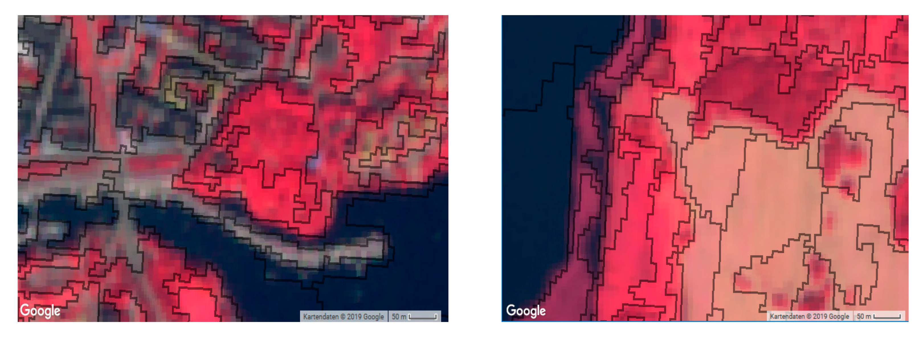
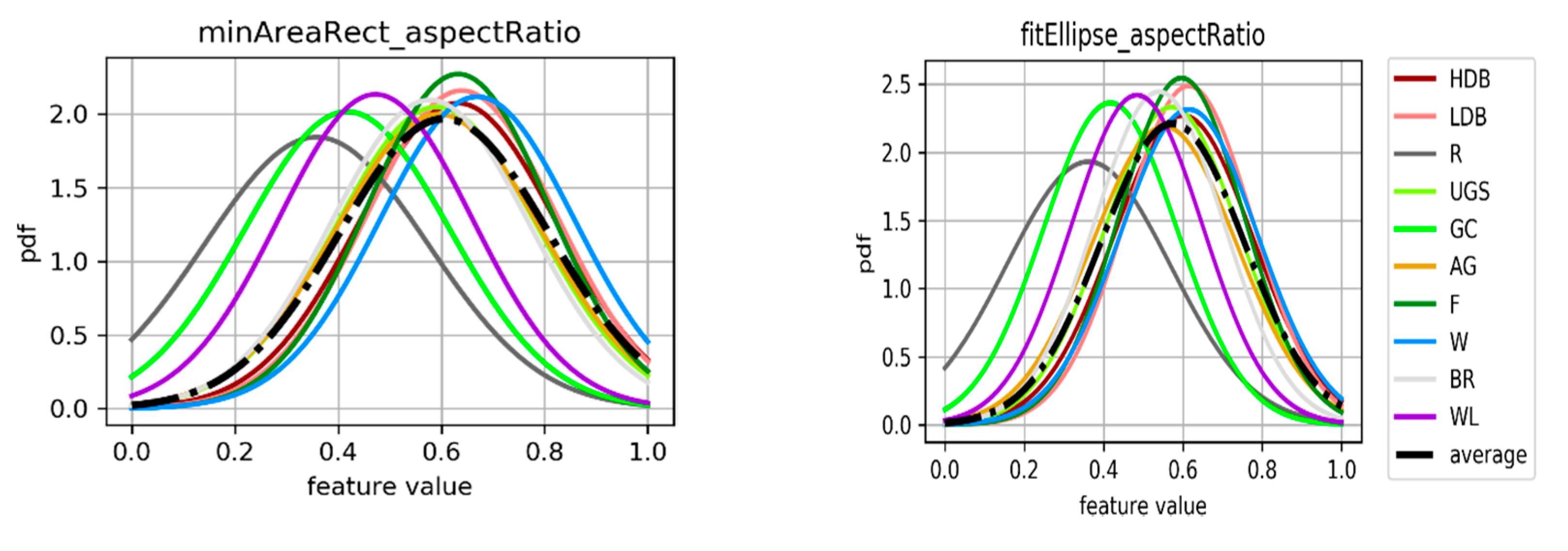
As mentioned earlier, an object-based approach has been adopted in order to reduce the computational burden and focus more on the feature selection and classification. The segmented image-objects should aim to depict the entities of the urban land cover types. For the detection of low-density built-up areas, which are a dense mix of built-up and vegetated pixels, an object-based approach is beneficial. Additionally, the separation of high-density built-up areas and roads can benefit from the geometric properties of the objects (e.g., minimum enclosing circle, minimal area rotated rectangle, and least-squared fitted ellipse).

For both study areas, the segmentation is performed using a multiresolution module of eCognition software [60]. The segmentation is based on the S2 10 m spectral bands. The segments are created using a scale parameter of 50, a shape vs. color ratio of 0.7:0.3 and a compactness vs. smoothness ratio of 0.7:0.3. The parameters were selected based on repeated tests for a subjectively good segmentation (compare Figure 2, Figure 3 and Figure 4). The criteria of this selection were mainly the proper distinction of segments containing LDB (low density built-up) in comparison to UGS (urban green spaces); and R (roads and railroads) in comparison to HDB (high density built-up). The adequacy of a segmentation layout can only be assessed in the context of an application. Consequently, the traditional approach has been to use human expert to evaluate the quality of the segmentation [59]. However, when facing big EO data, the segmentation process and determination of its parameters needs to be automated. Several approaches have been proposed [61,62,63] and should be evaluated for efficient integration in the workflow.

Using the reference data, the segments were labeled based on the class of the reference point located in the segment. Inside Stockholm lies a total of 5800 labeled segments and an additional 200,000 unlabeled segments (~3% labeled). In Beijing 1100 segments are labeled and 458,000 segments are unlabeled (~0.25% labeled). For Stockholm and Beijing, the analysis considers S1 and S2 images from the summer of 2015 and 2016, respectively (

Table 2. Overview of the acquired satellite imagery

Stockholm	Beijing
S1 imagery (15 Ascending, 12 Descending)	S1 imagery (11 Ascending, 18 Descending)
Period: 01-05-2015-–30-09-2015	Period: 01-05-2016–30-09-2016
Polarizations: VV, VH	Polarizations: VV, VH
S2 Imagery (8 Images)	S2 Imagery (11 Images)
Period: 01-06-2015–30-08-2015-	Period: 01-06-2016–30-09-2016
Cloudy pixels: <15%	Cloudy pixels: <15%

). For S1 images, two orbit directions (i.e., ascending and descending) with two polarizations (i.e., VV and VH) are used and treated as individual inputs. Four temporal stacks are created (one for each direction/polarization). Each temporal stack is reduced by computing its temporal mean and standard deviation. This way, the speckle noise is reduced while still capturing temporal variations of the different LULC classes. For each mean and standard deviation image, 17 GLCM texture measures (

Table 3. GLCM texture measures.

Band	Description	Band	Description
asm	angular second moment	contrast	contrast
corr	correlation	var	sum of squares: variance
idm	inverse difference moment	savg	sum average
svar	sum variance	sent	sum entropy
ent	entropy	dvar	difference variance
dent	difference entropy	imcorr1/imcorr2	information measures of correlation 1/2
diss	dissimilarity	inertia	inertia

) estimated with kernel size of 9 × 9 are computed. Finally, for each segment, the mean, standard deviation, max, and min of the abovementioned features are computed (see

Table 4. Overview of all generated features

Sensor	Input layers		Segment Statistics (Mean, Min, Max, Std.Dev)	No. of Features
S1	temporal mean		4 images (Asc/Desc VV/VH)	16
	temporal standard deviation		4 images (Asc/Desc VV/VH)	16
	texture features		8 images 17 GLCM features	544
S2	cloud-free composite		12 spectral bands	48
			2 spectral indices	8
	texture features NIR	10 m bands	1 band 17 GLCM features	68
geometry	minimum enclosing circle		radius, areal difference	2
	minimal area rotated rectangle		height, width, angle, aspect ratio, aereal difference	5
	least-squares-fitted ellipse		major-axis, minor-axis, angle, aspect ratio, areal difference	5
			Sum	712

).

The S2 stack is filtered such that only images with less than 15% cloud cover is included. All S2 spectral bands were resampled to 10 m spatial resolution. In addition to the 12 spectral bands, normalized difference-vegetation and water indices (NDVI, and NDWI) are computed and added to the S2 stack. Additionally, 17 GLCM texture measures are computed for NIR (10 m) spectral band: we could have computed GLCM textures for all S2 spectral band but this would have increased the number of features tremendously (extra 748 features) without adding substantial new information considering the high correlation of texture between the available S2 bands. Moreover, since several S1 textures have been included, choosing only NIR texture will be enough for the objective of this paper. For each segment, four statistics (i.e., mean, standard deviation, min, and max) are computed for all the available images. Finally, 12 features describing the segments’ geometric properties are computed (see Table 4 for details). In total, 712 features are computed in the GEE platform and exported into GCP (see Table 4).

3. Methodology

An overview of our workflow is presented in Figure 3. It consists of three main steps: (1) feature computation, (2) dimensionality reduction and classifier parameters estimation, and (3) classification. In the first step, segments and reference points are imported to GEE and input time series are chosen from GEE’s data catalogue. The segments are labeled based on the reference points. Features are computed as statistics for each segment and exported to GCP. Please refer to the previous section for more details about data preparation and features computation. In the second step, different dimensionality reduction methods are performed, and an exhaustive grid search is used to optimize the classifier hyperparameters [64]. The estimated hyperparameters are then used to train the classifier. The results are analyzed using a non-inferiority test to detect the best classifier using the least number of features. The generated reports and graphs give useful insights that can be used to refine the first step of feature computation and reduce the data load. If a satisfying classifier has been found, in (3) the prediction of the land cover classes is performed, and a resulting land cover map is produced in GEE.

3.1. Feature Set and Classifier Optimization

Step two is the most important step in the abovementioned workflow. Figure 4 shows this step in more details. It mainly consists of features selection/extraction step intertwined with a cross-validated exhaustive grid search for the optimum parameters of the machine learning model, i.e., the SVM. The outputs are a set of selected features together with the best cross-validated classifier as specified by a selected metric (i.e., overall accuracy) and a table of the full cross-validation results. The latter is used to find improved feature sets with the non-inferiority test. The workflow performs the following steps:

• The first step is to scale the input features. Scaling ensures that all features have the similar ranges of value, which are beneficial or even essential for some dimensionality reduction methods as well as for the SVM classifier. We applied scaler that uses the second and third quantiles of the data to rescale the data linearly in the range [0,1].
• The second step is a reduction of the feature set dimensionality either through the feature extraction or feature selection methods.
• Given the selected feature set, the last step is to find, via grid search, the optimum set of hyperparameters for the SVM classifier.

This workflow is computationally excessive operation, but as it consists of many independent operations it can be parallelized and thus be run efficiently on GCP using a virtual machine with many CPUs. The next few subsections describe these steps in more details.

3.1.1. Data Sets and Cross-Validation

For the optimization, only the labeled segments are relevant. Unlabeled segments are left aside until creating a final land cover classification map. The labeled segments are split into a set of training and testing data with a specified ratio. The testing set is withheld from the optimization step and is only used for a final assessment. The training set serves as an input to feature selection/extraction and grid search. A repeated stratified k-fold of the training set is performed for cross-validation. It splits with n repetitions the training set into k equally large folds while preserving the distribution of the target classes. Cross-validation is then performed by leaving out one of the folds for validation of the classifier that is trained on the remaining folds. The number of folds k should be chosen in consideration of the training set size and especially the number of samples in the least represented classes. The number of repetitions n should be set according to the available amount of time and the required certainty in the cross-validations.

3.1.2. Dimensionality Reduction Step

Because of the involved simplicity and fast implementation, we decided to test and evaluate three different methods in the dimensionality reduction step. In particular, we tested the linear discriminant analysis (LDA), mutual information (MI), and Fisher’s criterion (F-Score). LDA is a supervised feature extraction method that takes training sample categories into consideration [65,66]. The input feature space is projected onto a linear subspace of directions that maximize the separation between class means while minimize interclass variance [67]. The number of the output dimensions must necessarily be smaller than the number of classes, which usually results in high data compression. MI and F-Score are feature selection methods from the subgroup of univariate filters. In both techniques, a certain criterion is used to rank the features according to their relevance to the target classes, and the best K features are then selected. In MI the ranking criterion is the mutual information, which is a non-negative value, measuring the mutual dependency between two random variables. It is zero if and only if the two variables are strictly independent, higher values indicating higher dependency. MI utilizes a non-parametric entropy estimation from k-nearest neighbor distances [68]. F-Score rank a feature based on the ratio of the between classes variance to the within classes variances. It assigns high rank to features that maximizes the distance between classes and minimizes the within class variance. Unlike the MI, the F-Score cannot model non-linear dependencies [69].

3.1.3. SVM Hyperparameters Estimation

In this step, cross-validated guided exhaustive grid search over the specified SVM parameter values is implemented. The grid search requires a learning machine, i.e., a classifier, to guide the process and a parameter grid describing the classifier’s settings. For each combination of parameters, grid search fits the learning machine to the training data. It then performs a prediction on withheld data and assesses the accuracy using the overall accuracy. This is repeated for each combination of training sets as specified by the chosen cross-validation method.

3.1.4. Non-Inferiority Test

Non-inferiority testing is a modification of the traditional hypothesis testing framework. Primarily used in clinical studies to prove that new therapies do not perform significantly worse than established therapies, when they might offer advantages such as fewer side effects, lower cost, easier application, or fewer drug interactions. This concept can be transferred to the classification problem. There, the secondary benefits could be the reduction of data, of computational complexity or of the sensitivity to the training set size. We use the non-inferiority test to find a well-performing classifier that has the secondary benefit of achieving a higher reduction in dimensionality. In contrast to the traditional hypothesis test, the non-inferiority test formulates a null hypothesis that states that the efficacy of the new method is inferior to the efficacy of the old method within the chosen non-inferiority margin, while the alternative hypothesis states that the efficacy of the new method is greater or equal to the efficacy of the old method within the non-inferiority margin. In rejecting this null hypothesis, one can be certain that the new method does not perform worse than the old method. The implementation of the non-inferiority test uses a Student’s t-distribution and applies the Welch’s t-test for samples with unequal variances. This test is performed using the overall accuracy as the single metric. The two parameters for this test are the non-inferiority margin and the significance level α. The non-inferiority margin describes the acceptable deviation of efficacy from the best performing method. The significance level describes the certainty of the hypothesis test as probability of falsely rejecting the null hypothesis. Both should be carefully selected for the problem at hand. If the computed p-value < α, non-inferiority is established.

3.2. Classification

In the last step, after finding the best set of features (i.e., dimensionality reduction) and the optimum SVM hyperparameter values, the classifier is trained using the whole training data set and the land cover classes for all segments are predicted. The results are joined with the segment polygons in GEE and an appropriate color scheme is applied for the presentation of the final land cover map. Finally, the test set is used to independently evaluate the accuracy of the classification map.

4. Results and Discussion

4.1. Stockholm Study Area

The feature set is forwarded to a virtual machine on GCP, which is specified with 16 virtual Intel Haswell CPUs, 20 GB memory, and Ubuntu 16.04.4 LTS as operating system. The labeled segments were split into a training set of 70% and a withheld testing set of 30%, stratified by classes. The repeated stratified k-fold was set to three folds with three repetitions. This enables still a relatively large number of samples in each fold while enabling nine validations on the leave-one-out cross-validation.

The grid search is run separately for each feature extraction and feature selection method using the parameters shown in

Table 5. Parameter grid for the exhaustive grid search (Stockholm)

Method	Feature Range	$\mathit{C}$-Parameter			$\mathit{\gamma }$-Parameter
		Start	Stop	Num	Start	Stop	Num
Def.SVM	712	0	8	9	−10	−2	9
LDA	1–9	−1	5	7	−6	−1	6
MI	1–712	1	6	6	−9	−3	7
F-Score	1–712	1	7	7	−8	−2	7

. The feature range column indicates the range of numbers of features that have been tested (discriminants of the LDA are referred to as features for convenience). While Default SVM uses all features, the LDA can only generate maximum one component less than the number of classes, which is why the maximum range ends at 9. All other methods were tested for a set of 30 approximately logarithmically spaced numbers of features spanning from 1 to 712. The C-and γ-parameters are in a decadic space within the range of exponents indicated in the columns start and stop; the number of parameters to test is specified in the column num. The search space C and γ has been verified visually with heat maps, as shown in Figure 5. If the highest overall accuracy was achieved at the borders of the parameter ranges, the range was extended.

The best-performing classifiers identified by the grid search are presented in

Table 6. Overview of the best-performing classifiers (Stockholm)

	Mean Overall Accuracy [%]	Std. Dev. of Accuracy [%]	Accuracy Test Data [%]	Number of Features	Dimensionality Compression	Decrease Factor Training Time	Decrease Factor Pred. Time
Method	Best-performing classifier
Def.SVM	88.0	0.78	87.9	712	1	1	1
LDA	93.1	0.93	94.4	9	79	16	17
MI	94.4	0.64	94.7	185	4	6	10
F-Score	95.0	0.75	94.7	124	6	10	12
	Best-performing within 0.5% non-inferiority margin
LDA	-	-	-	-	-	-	-
MI	94.3	0.69	94.5	38	19	11	38
F-Score	84.9	0.43	94.9	102	7	10	10
	Best-performing within 1% non-inferiority margin
LDA	92.5	0.51	94.4	7	102	22	25
MI	93.6	0.36	94.3	31	23	4	43
F-Score	94.4	0.32	94.3	56	13	16	23
	Best-performing within 3% non-inferiority margin
LDA	91.3	0.54	92.3	5	142	48	58
MI	91.8	0.95	93.5	14	51	1	47
F-Score	92.3	0.65	93.7	14	51	19	45
	Best-performing within 5% non-inferiority margin
LDA	89.2	0.92	90.3	4	178	36	75
MI	89.9	0.83	91.4	9	79	1	44
F-Score	90.7	0.75	91.9	8	89	2	50

. It first shows the results without a non-inferiority test. Then the results with non-inferiority margins of 0.5%, 1%, 3%, and 5% respectively are shown. A significance level of 2.5% was chosen for the non-inferiority test. The mean overall accuracy and the standard deviation of overall accuracies are shown for the nine cross-validation results. Additionally, the overall accuracy of the prediction on the 30% withheld testing segments are shown. Furthermore, the table presents numbers of features used and hence the compression of dimensionality (i.e., total number of available features divided by number of features used). The mean training and prediction times—as measured during the grid search—are shown as decrease factors compared to the default SVM. The results without the non-inferiority test show that all methods achieved better accuracies and reduced computational costs compared to the Default SVM. In terms of data compression and training and prediction time, the LDA is unsurpassable. MI and F-Score achieve the highest accuracy values on the withheld testing data; however, both still use much more features. Inside a 0.5% non-inferiority margin, MI and F-Score achieve a higher dimensionality compression, while keeping a high accuracy on withheld testing data, or in the case of F-Score even surpassing the initial result. No LDA with fewer features was found inside the 0.5% margin. When the non-inferiority margin is extended, higher dimensionality compressions can be achieved, however the accuracy on withheld testing data slightly decreases. Even with a large margin of 5%, all methods outperform the Default SVM on the withheld testing data, while achieving a drastic reduction of the dimensionality. It can also be noted that all methods apart from the Default SVM achieve higher accuracies on the withheld testing data than on the training data in the cross-validation.

Taking a closer look at the results for the individual methods, the influence of the number of features can be visualized: Figure 6 shows the classifier performances during the cross-validation in the grid search highlighting the mean overall accuracy with shaded areas representing ±3σ. It can be observed that LDA surpasses the default SVM’s accuracy with less than five components and reaches its maximum with all possible components (one less than the number of classes). MI shows a large variance especially when few features are used. It surpasses the results of the Default SVM between 5 and 10 selected features and achieves more reliable results with less variance thereafter. Between 30 and 500 selected features it shows an almost constant behavior. It seems that more features neither improve nor harm the classifier’s performance. F-Score is more stable than MI when few features are used, though it achieves lower accuracy scores. The default SVM is surpassed with fewer features than MI and in general there is less variance in the performance while obtaining similar accuracy scores. Only when more than 500 features are included, MI and F-Score, as expected, fall back to the performance of the default SVM.

Taking a closer look at the results for the individual methods, the influence of the number of features can be visualized: Figure 6 shows the classifier performances during the cross-validation in the grid search highlighting the mean overall accuracy with shaded areas representing ±3σ. It can be observed that LDA surpasses the default SVM’s accuracy with less than five components and reaches its maximum with all possible components (one less than the number of classes). MI shows a large variance especially when few features are used. It surpasses the results of the default SVM between 5 and 10 selected features and achieves more reliable results with less variance thereafter. Between 30 and 500 selected features it shows an almost constant behavior. It seems that more features neither improve nor harm the classifier’s performance. F-Score is more stable than MI when few features are used, though it achieves lower accuracy scores. The default SVM is surpassed with fewer features than MI and in general there is less variance in the performance while obtaining similar accuracy scores. Only when more than 500 features are included, MI and F-Score, as expected, fall back to the performance of the default SVM.

Figure 7 shows the confusion matrices of the prediction of the withheld testing data for the different classifiers at 0% non-inferiority-margin. The default SVM shows a high shift from roads to HDB but also from UGS to LDB and HDB and from bare rock to forests and HDB. It is notable that the shift is dominant in the direction of well-represented classes (compare Table 1).

All methods, LDA, MI, and F-Score, can remove some of these confusions. LDA reduces the shift from roads to HDB best but cannot avoid it completely, F-Score just slightly improves it, while MI shows only a minor improvement.

Roads and HDB have a very similar signature response and they are the most challenging classes in the presented classification schema; moreover, the spatial resolution of Sentinels imagery (10–20 m) is not sufficient to detect small roads. These are the main reasons why there is a higher confusion among these two classes across the results. The shifts from UGS and bare rock are reduced by all methods and best by F-Score. The default SVM achieves high accuracies of more than 90% on the remaining classes, however every method improves these further, reaching up to 99% and 100% for forest, water, and wetland classes.

In general, the main data processing advantage of the proposed framework is to use GEE and GCP to reduce the computational time and the download and preprocessing time to handle S1 and S2 dense time series. GEE is efficient in producing the feature data and is free of charge for non-commercial applications; GCP can be configured to have a good balance between computational power vs. operational costs. The main bottleneck for integration of GEE and GCP is the data transmission between the two platforms; however, it is the only technical solution that we found to combine the GEE platform with advanced machine learning libraries (i.e., scikit-learn). Moreover, we adopted an object-based approach and computed all the object statistics directly in the GEE platform. Hence, we only transfer a small amount of data between these two platforms (around 200,000 sample statistics in Stockholm case for example) limiting the side effect of data transfer. Figure 8 depicts the prediction times over the number of features for the different methods. For comparison, the times of the default SVM are is shown as dashed black line. It can be observed that LDA outperforms the default SVM drastically in prediction times. The figure clearly shows the expected outcome, i.e., the prediction time grows exponentially with number of features.

To analyze sensitivity to the training set size, learning curves are generated. Plotting the training and testing accuracy over adjusted training set sizes can give an indication of how training set size affects the classifier’s accuracy. Figure 9 shows the learning curves for the different classifiers at 0% non-inferiority margin using 2% to 70% of the initial training set. All learning curves have been cross-validated with six stratified shuffled splits, withholding 30% for testing. Shaded areas indicate ±3σ of the overall accuracy. As might be expected, the accuracy of the default SVM is worst with the smallest training set size. With an increasing training set size, the testing accuracy increases while showing less variance and the training score decreases slightly. The gap between both scores at the largest training set size indicates that this classifier could still be improved with the further addition of training samples.

LDA shows a remarkably unstable behavior for variable training set sizes. Though it achieves reasonable testing scores on very small training set sizes, its performance drops drastically for medium-sized training sets. Only with very large training sets does the accuracy reach the level seen in Figure 8. We assume that the between-class scatter matrix is becoming singular for this specific number of around 500 training samples, which is a known problem when there are less training samples than input dimensions [70]. One explanation could be that LDA is more sensitive to the quality of the training samples. Note that, for a given size, the training samples are selected randomly and could therefore not be representative of all the classes. The remaining gap between training scores and testing scores shows that this classifier could further be improved with larger and more balanced training sets. In fact, the decline in the training score is just starting to become visible at the largest training sets.

LDA shows a remarkably unstable behavior for variable training set sizes. Though it achieves reasonable testing scores on very small training set sizes, its performance drops drastically for medium-sized training sets. Only with very large training sets does the accuracy reach the level seen in Figure 8. We assume that the between-class scatter matrix is becoming singular for this specific number of around 500 training samples, which is a known problem when there are less training samples than input dimensions [70]. One explanation could be that LDA is more sensitive to the quality of the training samples. Note that, for a given size, the training samples are selected randomly and could therefore not be representative of all the classes. The remaining gap between training scores and testing scores shows that this classifier could further be improved with larger and more balanced training sets. In fact, the decline in the training score is just starting to become visible at the largest training sets.

The testing scores for MI and F-Score already surpass the default SVM at the smallest training set size. The F-Score shows slightly larger variances on the testing score compared to MI, indicating its higher dependency on meaningful training samples. The accuracy of both methods can be increased with larger training set sizes. However, compared to the default SVM the gap between training and testing scores is smaller and the convergence can clearly be seen. Figure 10 shows the S1 temporal mean VV-VH-composite, the S2 false-color composite and one of the predicted land cover maps with F-Score feature selection using 102 features.

4.2. Beijing Study Area

The split of 70% training and 30% testing set was performed in the same way as in the Stockholm study area and the same cross-validation method and parameters were chosen. However, the parameters needed to be adjusted. More specifically, the maximum number of features used for the LDA had to be reduced to 7 accordingly with the number of classes and the search ranges for the C-and γ-parameters had to be adjusted to find the optimal hyperparameters as indicated in

Table 7. Parameter grid for the exhaustive grid search (Beijing).

Method	Feature Range	$\mathit{C}$-Parameter			$\mathit{\gamma }$-Parameter
		Start	Stop	Num	Start	Stop	Num
Def.SVM	712	3	11	9	−12	−4	9
LDA	1–7	−1	5	7	−7	−1	7
MI	1–712	3	8	6	−9	−4	6
F-Score	1–712	2	8	7	−10	−3	8

.

Table 8. Overview of the best performing classifiers (Beijing)

	Mean Overall Accuracy [%]	Std. Dev. of Accuracy [%]	Accuracy Test Data [%]	Number of Features	Dimensionality Compression	Decrease Factor Training Time	Decrease Factor Pred. Time
Method	Best-performing classifier
Def.SVM	76.0	6.97	81.9	712	1	1	1
LDA	84.4	3.62	77.5	7	102	5	14
MI	91.5	2.64	90	226	3	3	4
F-Score	93.7	2.43	93.1	226	3	3	4
	Best-performing within 3% non-inferiority margin
LDA	-	-	-	-	-	-	-
MI	89.9	2.42	88.1	13	55	1	16
F-Score	91.6	2.42	90	110	6	3	7
	Best-performing within 5% non-inferiority margin
LDA	81.9	3.93	77.5	6	119	5	13
MI	87.7	2.55	89.4	10	71	1	16
F-Score	89.7	1.01	93.1	21	34	4	13

shows the best classifiers found by the grid search, again without and with a non-inferiority margin. In contrast to the Stockholm study area, no better classifiers were found within non-inferiority margins of 0.5% or 1%, hence only 3% and 5% margins are presented. The performances of all classifiers are worse and less stable than in the Stockholm study area. Considering the learning curves in Figure 9, this behavior is not surprising considering the smaller training set of this study area. The Default SVM only reaches a mean overall accuracy of 76% on the training set and shows a very large standard deviation of almost 7%. On the withheld testing set, this performance is only marginally better. LDA achieves higher mean overall accuracies on the training set than the default SVM, it performs very poorly (77.5% overall accuracy) on the testing set, both with seven and six features. Considerably better, are MI’s and F-Score’s results. While both show a high instability on their performance with a standard deviation of around 2.5%, their overall accuracy surpasses 90%. Inside the 3% non-inferiority margin, MI can be reduced from 226 to 13 features, however the accuracy is reduced below 90%. F-Score still uses 110 features and achieves an accuracy of just 90% on the withheld data. With a 5% margin, MI is further reduced to 10 features, with a slightly increasing accuracy on withheld data compared to the 3% margin. F-Score is reduced to 21 features and achieves the same accuracy on the withheld testing data as without a non-inferiority margin.

It can be observed by comparing Figure 8 and Figure 11 that all three methods perform worse in Beijing than in Stockholm and show a higher instability. As expected, with the smaller training set size, it is more difficult to find a good classifier and a good subset of features. LDA surpasses the default SVM just slightly, when all seven features are used, but still shows a large variance at that point. MI and F-Score can both surpass the default SVM in a similar way as for the Stockholm study area. Once past the default SVM accuracy, MI reaches higher accuracy scores with fewer features than F-Score. Thus, F-Score appears to be more sensitive to the combination of few features and small training sets. The normalized confusion matrices in Figure 12 show that the default SVM has a high shift from LDB to HDB and roads, from UGS to agriculture, from golf courses to UGS, and from agriculture to forests and HDB. LDA cannot reduce these confusions and introduces new errors. Many segments were falsely predicted as forests. Overall, MI and F-Score improve these classification results and are able to reduce confusions.

4.3. Comparison of the Study Areas

Whereas all methods-LDA, MI, and F-Score-could improve the classification accuracies in the case study of Stockholm with a comparably large training set size, LDA appears to be unsuited for cases with small training set sizes as in Beijing. The estimation of the class means and variances is essential for LDA and thus a sufficiently large training set is required. MI and F-Score work reasonably well also with smaller training sets. However, all methods produced more stable results in Stockholm than in Beijing.

Figure 13 visualizes an excerpt from the feature ranking by MI and F-Score. The top 20 features averaged over both methods are presented grouped by S1 and S2 for Stockholm and Beijing. This ranking was created with cross-validation of five stratified folds of the whole training set. The averaged rank is indicated next to the feature name. MI and F-Score rank the features differently as they are using different measures. It is interesting, but not surprising, to see that the features from descending and ascending S1 passes are always paired up in this ranking. VV polarizations appear to be slightly more informative than VH polarizations, as the same features always appear in the same order for the respective polarizations. Another interesting observation is that the VV_mean has a very high rank in general. SAR response is very sensitive to geometric properties of the observed objects and could therefore, help discriminating between certain LULC classes especially in the urban environment. As an example, built-up areas are characterized by double bounce scattering, and consequently, appear very bright unlike roads with their smooth surface, which appear very dark in radar images.

The highest-ranking features from S2 are the indices NDVI and NDWI. They are followed by red edge, near- and short-wave-infrared bands (B6-B11). The first feature from the visible spectrum was the mean of B4 (red) that held rank 54 in Stockholm and rank 30 in Beijing. The GLCM sum average (savg) delivers the highest ranked textural feature and appears for several bands in the top 20 ranking. Even though the rankings are not exactly the same, the results appear to be consistent for the different study areas—the same or similar features received the highest ranks. This is especially noteworthy as the accuracy scores in the study area of Beijing are way lower and more unstable than in Stockholm. Still the cross-validated, averaged feature importance ranking is quite similar.

The geometric features received low scores in this ranking and were hence excluded from Figure 13. In the Stockholm study area, the first geometric feature, the width of the fitted ellipse, was placed on rank 288. Two features, which were anticipated to reduce the confusion between roads and HDB, the aspect ratios of the minimum area rectangle and the fitted ellipse, were placed on rank 579 and 591 respectively. Inspecting the value distributions for these two features in Figure 14, it can be seen that they are useful to separate specific classes (roads, golf courses, and wetlands) but they do not contain useful information for the separation of the remaining classes. These features could be used rather for rule-based post-classification corrections to reduce the confusions between roads and HDB.

What should be considered for this ranking is that MI and F-Score are univariate feature selection methods, which do not account for correlation between the features. Thus, they do not detect redundancy in the feature set. Plotting the training samples for the two highest-ranking S1 features, it becomes obvious that they have a positive correlation (Figure 15). The plot for the highest-ranking S2 features shows a strong negative correlation. However, it is interesting to plot the highest-ranked S1 and S2 features; the separation of the classes becomes clearly visible showing the great potential of merging multispectral and SAR data.

5. Conclusions

This study demonstrates the feasibility of GEE and GCP infrastructure to apply dimensionality reduction through feature extraction and feature selection methods for object-based land cover classifications with oversized feature sets. The presented workflow allows thorough assessments of different features as well as different dimensionality reduction methods for specific GEOBIA applications. It incorporates the dimensionality reduction as a key step in the land cover classification process, which we consider essential for the exploitation of the growing EO big data.

The LDA showed the highest compression of the initial feature space and can obtain remarkable results in comparison to the default SVM. One disadvantage, however, is that this method gives no intuitive indication about the contribution of individual features to the accuracy and is less reliable with small training sets. The feature selection methods appear very promising and provide exactly this insight into the features’ quality. With a sensitive non-inferiority margin, both MI and F-Score allowed high compressions of the feature set and achieved notable improvements of the accuracy. This emphasizes the fact that dimensionality reduction should form a key step in land cover classification using SVM. Thanks to the availability of cloud computing, these dimensionality reduction processes are no longer limited by the lack of computational power and can easily be integrated into the classification workflow.

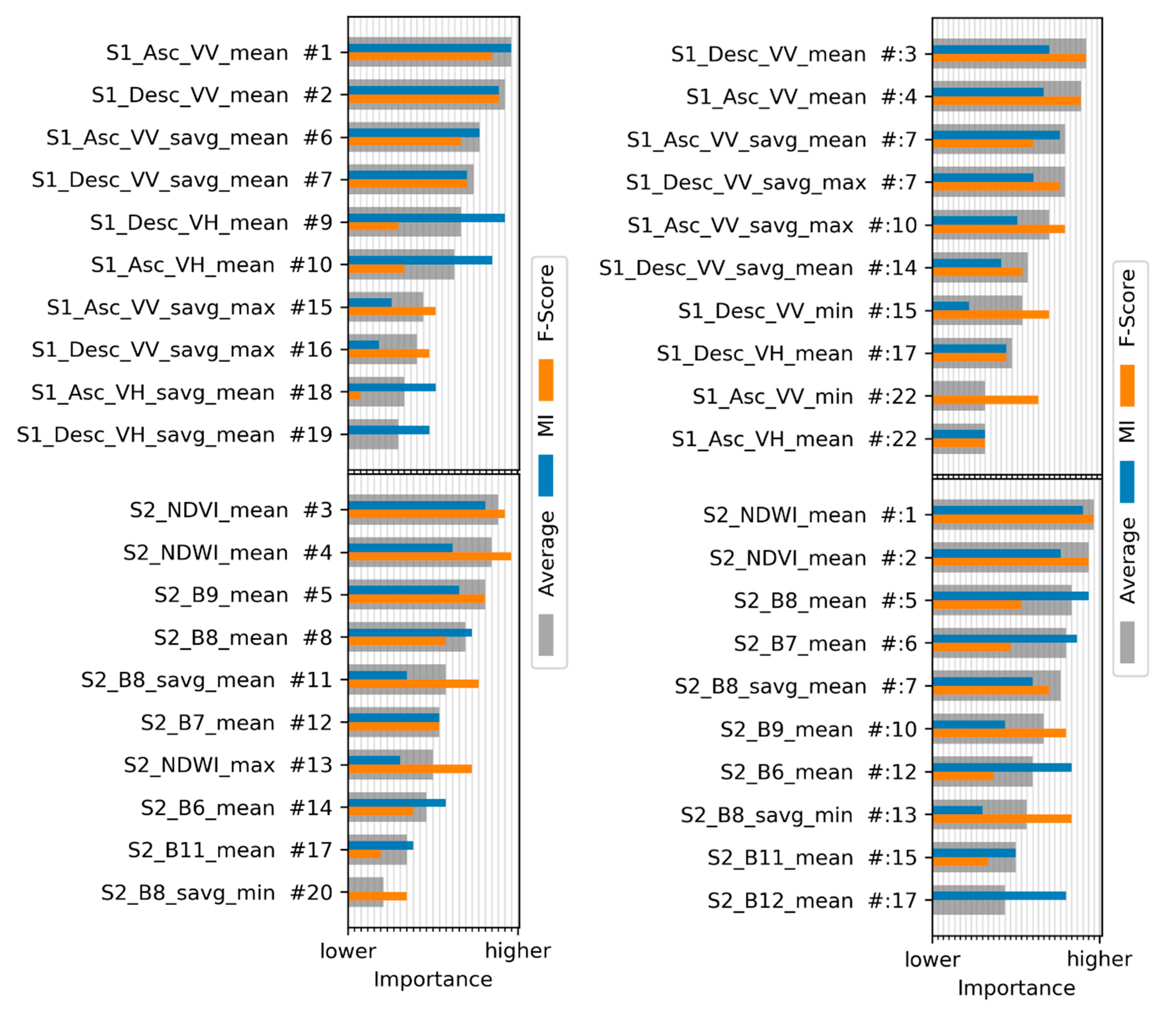
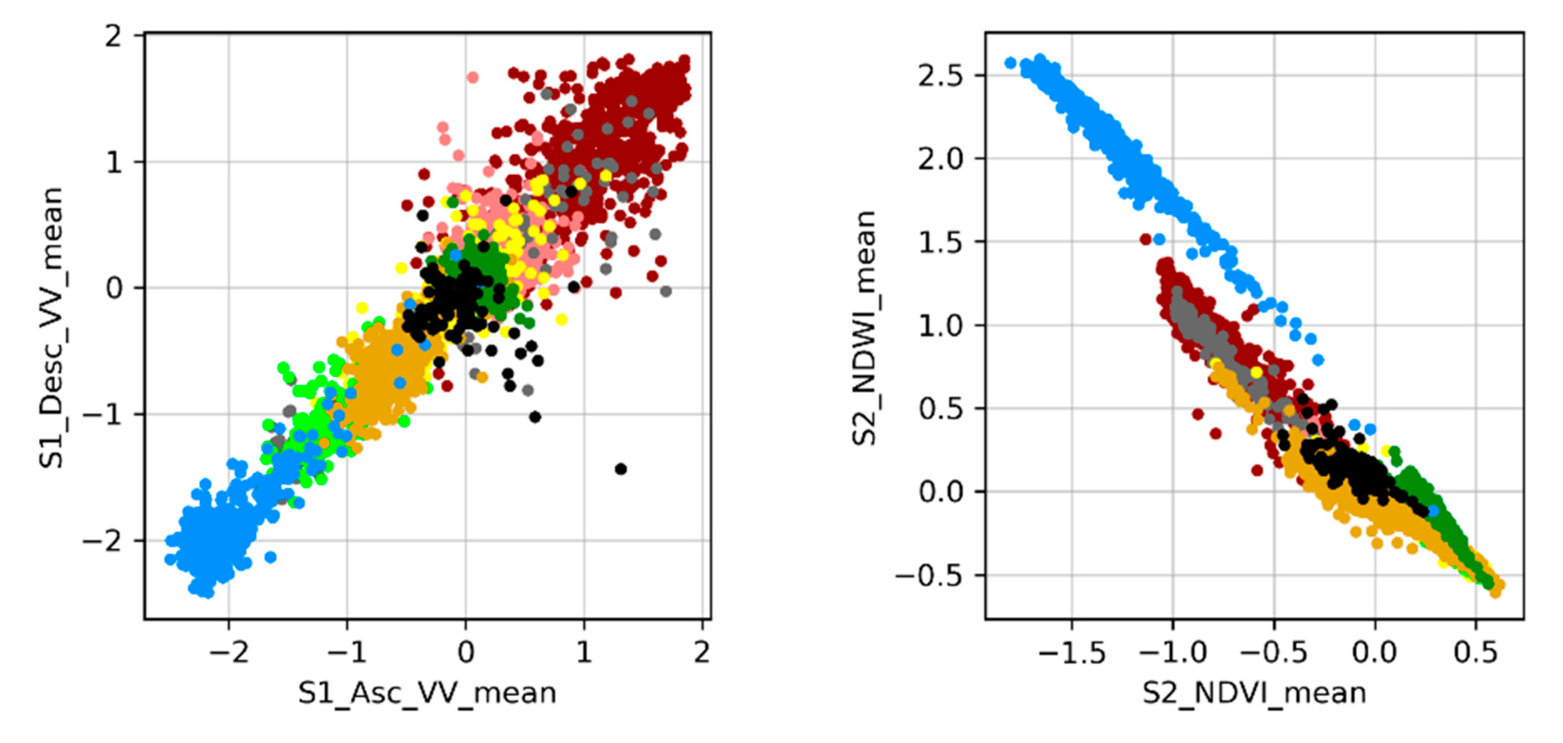
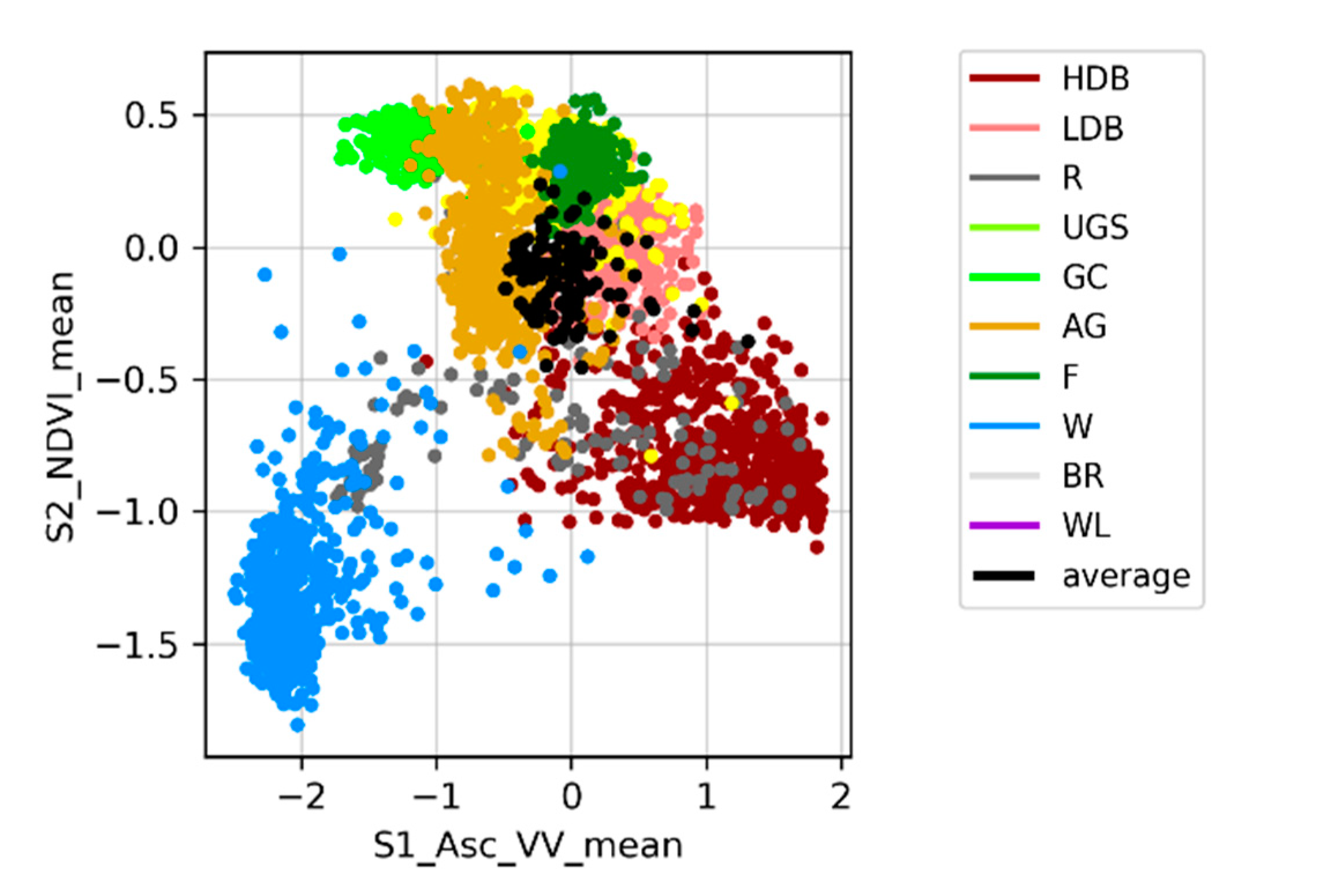
Despite the different training set sizes in the two study areas, the averaged feature importance ranking showed similar results for the top-ranking features. It strongly indicates that a feature-level fusion of SAR data from Sentinel-1 and multispectral imagery from Sentinel-2 allows for a better discrimination between different LULC classes. It should be acknowledged, however, that the optimal set of features is specific for each classification scheme. Different land cover classes require different features to be separable from one another. Future research should therefore expand this method to different classification schemes but also further investigate the importance of features for each individual class. To explore the relevance of features for a land cover classification more broadly, additional features need to be included in the analysis. More spectral indices should be included; thorough multi-temporal analyses of optical or SAR imagery are promising candidates to improve land cover; analysis of the phenology through harmonic or linear fitting of the NDVI, for example, help to distinguish between different vegetation classes.

Despite their limitation, LDA, MI, and F-Score serve as a demonstration of the integration in the workflow. In future work, different feature selection methods should be tested following the proposed methodology. Multivariate filter methods, in particular, should be explored, since the applied univariate methods fail to identify the dependency between similar high-ranked features. Moreover, wrappers and embedded methods especially designed for the chosen classifier should be included in the analysis as well.

Considering the multiple types of sensors and the massive amount of data that is already available and that will be available in the next years, we think that the developed framework can be used to analyze the importance of the different input data and the derived features; it can contribute to understanding how to optimize the integration of these different data sources (i.e., very high-resolution SAR and multispectral data) for object-based classification analysis.

The Python scripts developed during this study are released in a public GitHub repository and licensed under GNU GPL v3.0 [71]. Additionally, the respective JavaScript snippets for the Google Earth Engine web API as well as the segmented image-objects and reference points are published and referenced in the GitHub repository. We hope that this might encourage further research and the development of reliable workflows for the efficient exploitation of today’s EO big data with inter-comparable results.

References

1. Haack, B.; Bryant, N.; Adams, S. An assessment of landsat MSS and TM data for urban and near-urban land-cover digital classification. Remote Sens. Environ. 1987, 21, 201–213. [Google Scholar] [CrossRef]
2. Quarmby, N.A.; Cushnie, J.L. Monitoring urban land cover changes at the urban fringe from SPOT HRV imagery in south-east England. Int. J. Remote Sens. 1989, 10, 953–963. [Google Scholar] [CrossRef]
3. Zha, Y.; Gao, J.; Ni, S. Use of normalized difference built-up index in automatically mapping urban areas from TM imagery. Int. J. Remote Sens. 2003, 24, 583–594. [Google Scholar] [CrossRef]
4. Choi, J. A hybrid approach to urban land use/cover mapping using Landsat 7 Enhanced Thematic Mapper Plus (ETM+) images. Int. J. Remote Sens. 2004, 25, 2687–2700. [Google Scholar] [CrossRef]
5. Yuan, F.; Sawaya, K.E.; Loeffelholz, B.C.; Bauer, M.E. Land cover classification and change analysis of the Twin Cities (Minnesota) Metropolitan Area by multitemporal Landsat remote sensing. Remote Sens. Environ. 2005, 98, 317–328. [Google Scholar] [CrossRef]
6. Zhong, P.; Wang, R. A Multiple Conditional Random Fields Ensemble Model for Urban Area Detection in Remote Sensing Optical Images. IEEE Trans. Geosci. Remote Sens. 2007, 45, 3978–3988. [Google Scholar] [CrossRef]
7. Pierce, L.E.; Ulaby, F.T.; Sarabandi, K.; Dobson, M.C. Knowledge-based classification of polarimetric SAR images. IEEE Trans. Geosci. Remote Sens. 1994, 32, 1081–1086. [Google Scholar] [CrossRef]
8. Dell’Acqua, F.; Gamba, P. Discriminating urban environments using multiscale texture and multiple SAR images. Int. J. Remote Sens. 2006, 27, 3797–3812. [Google Scholar] [CrossRef]
9. Dell’Acqua, F.; Gamba, P. Texture-based characterization of urban environments on satellite SAR images. IEEE Trans. Geosci. Remote Sens. 2003, 41, 153–159. [Google Scholar] [CrossRef]
10. Brenner, A.R.; Roessing, L. Radar Imaging of Urban Areas by Means of Very High-Resolution SAR and Interferometric SAR. IEEE Trans. Geosci. Remote Sens. 2008, 46, 2971–2982. [Google Scholar] [CrossRef]
11. Niu, X.; Ban, Y. Multi-temporal RADARSAT-2 polarimetric SAR data for urban land-cover classification using an object-based support vector machine and a rule-based approach. Int. J. Remote Sens. 2013, 34, 1–26. [Google Scholar] [CrossRef]
12. Salehi, M.; Sahebi, M.R.; Maghsoudi, Y. Improving the Accuracy of Urban Land Cover Classification Using Radarsat-2 PolSAR Data. IEEE J. Sel. Top. Appl. Earth Obs. Remote Sens. 2014, 7, 1394–1401. [Google Scholar] [CrossRef]
13. Zhou, Y.; Wang, H.; Xu, F.; Jin, Y. Polarimetric SAR Image Classification Using Deep Convolutional Neural Networks. IEEE Geosci. Remote Sens. Lett. 2016, 13, 1935–1939. [Google Scholar] [CrossRef]
14. Dekker, R.J. Texture analysis and classification of ERS SAR images for map updating of urban areas in The Netherlands. IEEE Trans. Geosci. Remote Sens. 2003, 41, 1950–1958. [Google Scholar] [CrossRef]
15. Su, W.; Li, J.; Chen, Y.; Liu, Z.; Zhang, J.; Low, T.M.; Suppiah, I.; Hashim, S.A.M. Textural and local spatial statistics for the object-oriented classification of urban areas using high resolution imagery. Int. J. Remote Sens. 2008, 29, 3105–3117. [Google Scholar] [CrossRef]
16. Engdahl, M.E.; Hyyppa, J.M. Land-cover classification using multitemporal ERS-1/2 InSAR data. IEEE Trans. Geosci. Remote Sens. 2003, 41, 1620–1628. [Google Scholar] [CrossRef]
17. Guerschman, J.P.; Paruelo, J.M.; Bella, C.D.; Giallorenzi, M.C.; Pacin, F. Land cover classification in the Argentine Pampas using multi-temporal Landsat TM data. Int. J. Remote Sens. 2003, 24, 3381–3402. [Google Scholar] [CrossRef]
18. Camps-Valls, G.; Gomez-Chova, L.; Munoz-Mari, J.; Rojo-Alvarez, J.L.; Martinez-Ramon, M. Kernel-Based Framework for Multitemporal and Multisource Remote Sensing Data Classification and Change Detection. IEEE Trans. Geosci. Remote Sens. 2008, 46, 1822–1835. [Google Scholar] [CrossRef]
19. Tigges, J.; Lakes, T.; Hostert, P. Urban vegetation classification: Benefits of multitemporal RapidEye satellite data. Remote Sens. Environ. 2013, 136, 66–75. [Google Scholar] [CrossRef]
20. Waske, B.; van der Linden, S. Classifying Multilevel Imagery from SAR and Optical Sensors by Decision Fusion. IEEE Trans. Geosci. Remote Sens. 2008, 46, 1457–1466. [Google Scholar] [CrossRef]
21. Amarsaikhan, D.; Blotevogel, H.H.; Genderen, J.L.; van Ganzorig, M.; Gantuya, R.; Nergui, B. Fusing high-resolution SAR and optical imagery for improved urban land cover study and classification. Int. J. Image Data Fusion 2010, 1, 83–97. [Google Scholar] [CrossRef]
22. Corbane, C.; Faure, J.-F.; Baghdadi, N.; Villeneuve, N.; Petit, M. Rapid Urban Mapping Using SAR/Optical Imagery Synergy. Sensors 2008, 8, 7125–7143. [Google Scholar] [CrossRef] [PubMed]
23. Pacifici, F.; Frate, F.D.; Emery, W.J.; Gamba, P.; Chanussot, J. Urban Mapping Using Coarse SAR and Optical Data: Outcome of the 2007 GRSS Data Fusion Contest. IEEE Geosci. Remote Sens. Lett. 2008, 5, 331–335. [Google Scholar] [CrossRef] [Green Version]
24. Ban, Y.; Yousif, O.; Hu, H. Fusion of SAR and Optical Data for Urban Land Cover Mapping and Change Detection. In Global Urban Monitoring and Assessment through Earth Observation; Weng, Q., Ed.; CRC Press: Boca Raton, FL, USA, 2014; pp. 353–386. [Google Scholar] [CrossRef]
25. Makarau, A.; Palubinskas, G.; Reinartz, P. Multi-sensor data fusion for urban area classification. In Proceedings of the 2011 Joint Urban Remote Sensing Event, Munich, Germany, 11–13 April 2011; pp. 21–24. [Google Scholar] [CrossRef] [Green Version]
26. Zhang, H.; Lin, H.; Li, Y. Impacts of Feature Normalization on Optical and SAR Data Fusion for Land Use/Land Cover Classification. IEEE Geosci. Remote Sens. Lett. 2015, 12, 1061–1065. [Google Scholar] [CrossRef]
27. Zhang, Y.; Zhang, H.; Lin, H. Improving the impervious surface estimation with combined use of optical and SAR remote sensing images. Remote Sens. Environ. 2014, 141, 155–167. [Google Scholar] [CrossRef]
28. Zhu, Z.; Woodcock, C.E.; Rogan, J.; Kellndorfer, J. Assessment of spectral, polarimetric, temporal, and spatial dimensions for urban and peri-urban land cover classification using Landsat and SAR data. Remote Sens. Environ. Remote Sens. Urban Environ. 2012, 117, 72–82. [Google Scholar] [CrossRef]
29. Ban, Y.; Hu, H.; Rangel, I.M. Fusion of Quickbird MS and RADARSAT SAR data for urban land-cover mapping: object-based and knowledge-based approach. Int. J. Remote Sens. 2010, 31, 1391–1410. [Google Scholar] [CrossRef]
30. Myint, S.W.; Gober, P.; Brazel, A.; Grossman-Clarke, S.; Weng, Q. Per-pixel vs. object-based classification of urban land cover extraction using high spatial resolution imagery. Remote Sens. Environ. 2011, 115, 1145–1161. [Google Scholar] [CrossRef]
31. Bruce, L.M.; Koger, C.H.; Li, J. Dimensionality reduction of hyperspectral data using discrete wavelet transform feature extraction. IEEE Trans. Geosci. Remote Sens. 2002, 40, 2331–2338. [Google Scholar] [CrossRef]
32. Harsanyi, J.C.; Chang, C.-I. Hyperspectral image classification and dimensionality reduction: an orthogonal subspace projection approach. IEEE Trans. Geosci. Remote Sens. 1994, 32, 779–785. [Google Scholar] [CrossRef] [Green Version]
33. Laliberte, A.S.; Browning, D.M.; Rango, A. A comparison of three feature selection methods for object-based classification of sub-decimeter resolution UltraCam-L imagery. Int. J. Appl. Earth Obs. Geoinf. 2012, 15, 70–78. [Google Scholar] [CrossRef]
34. Lennon, M.; Mercier, G.; Mouchot, M.C.; Hubert-Moy, L. Independent component analysis as a tool for the dimensionality reduction and the representation of hyperspectral images. In Proceedings of the IGARSS 2001. Scanning the Present and Resolving the Future. IEEE 2001 International Geoscience and Remote Sensing Symposium (Cat. No.01CH37217), Sydney, Australia, 9–13 July 2001; pp. 2893–2895. [Google Scholar] [CrossRef] [Green Version]
35. Ren, J.; Zabalza, J.; Marshall, S.; Zheng, J. Effective Feature Extraction and Data Reduction in Remote Sensing Using Hyperspectral Imaging [Applications Corner]. IEEE Signal Process. Mag. 2014, 31, 149–154. [Google Scholar] [CrossRef] [Green Version]
36. Van Coillie, F.M.B.; Verbeke, L.P.C.; De Wulf, R.R. Feature selection by genetic algorithms in object-based classification of IKONOS imagery for forest mapping in Flanders, Belgium. Remote Sens. Environ. For. Spec. Issue 2007, 110, 476–487. [Google Scholar] [CrossRef]
37. Guyon, I.; Elisseeff, A. An Introduction to Variable and Feature Selection. J. Mach. Learn. Res. 2003, 3, 1157–1182. [Google Scholar]
38. Eklundh, L.; Singh, A. A comparative analysis of standardised and unstandardised Principal Components Analysis in remote sensing. Int. J. Remote Sens. 1993, 14, 1359–1370. [Google Scholar] [CrossRef]
39. Du, Q. Modified Fisher’s Linear Discriminant Analysis for Hyperspectral Imagery. IEEE Geosci. Remote Sens. Lett. 2007, 4, 503–507. [Google Scholar] [CrossRef]
40. Martínez, A.M.; Kak, A.C. PCA versus LDA. IEEE Trans. Pattern Anal. Mach. Intell. 2001, 23, 228–233. [Google Scholar] [CrossRef] [Green Version]
41. Cao, L.J.; Chua, K.S.; Chong, W.K.; Lee, H.P.; Gu, Q.M. A comparison of PCA, KPCA and ICA for dimensionality reduction in support vector machine. Neurocomputing 2003, 55, 321–336. [Google Scholar] [CrossRef]
42. Li, J.; Cheng, K.; Wang, S.; Morstatter, F.; Trevino, R.P.; Tang, J.; Liu, H. Feature Selection: A Data Perspective. ACM Comput. Surv. 2017, 50, 1–45. [Google Scholar] [CrossRef] [Green Version]
43. Gorelick, N.; Hancher, M.; Dixon, M.; Ilyushchenko, S.; Thau, D.; Moore, R. Google Earth Engine: Planetary-scale geospatial analysis for everyone. Remote Sens. Environ. 2017, 202, 18–27. [Google Scholar] [CrossRef]
44. Pedregosa, F.; Varoquaux, G.; Gramfort, A.; Michel, V.; Thirion, B.; Grisel, O.; Blondel, M.; Müller, A.; Nothman, J.; Louppe, G.; et al. Scikit-learn: Machine Learning in Python. arXiv 2012, arXiv:1201.0490. [Google Scholar]
45. Buitinck, L.; Louppe, G.; Blondel, M.; Pedregosa, F.; Mueller, A.; Grisel, O.; Niculae, V.; Prettenhofer, P.; Gramfort, A.; Grobler, J.; et al. API design for machine learning software: experiences from the scikit-learn project. arXiv 2013, arXiv:1309.0238. [Google Scholar]
46. Mountrakis, G.; Im, J.; Ogole, C. Support vector machines in remote sensing: A review. ISPRS J. Photogramm. Remote Sens. 2011, 66, 247–259. [Google Scholar] [CrossRef]
47. Melgani, F.; Bruzzone, L. Classification of hyperspectral remote sensing images with support vector machines. IEEE Trans. Geosci. Remote Sens. 2004, 42, 1778–1790. [Google Scholar] [CrossRef] [Green Version]
48. Tarabalka, Y.; Fauvel, M.; Chanussot, J.; Benediktsson, J.A. SVM- and MRF-Based Method for Accurate Classification of Hyperspectral Images. IEEE Geosci. Remote Sens. Lett. 2010, 7, 736–740. [Google Scholar] [CrossRef] [Green Version]
49. Huang, X.; Zhang, L. An SVM Ensemble Approach Combining Spectral, Structural, and Semantic Features for the Classification of High-Resolution Remotely Sensed Imagery. IEEE Trans. Geosci. Remote Sens. 2013, 51, 257–272. [Google Scholar] [CrossRef]
50. Nemmour, H.; Chibani, Y. Multiple support vector machines for land cover change detection: An application for mapping urban extensions. ISPRS J. Photogramm. Remote Sens. 2006, 61, 125–133. [Google Scholar] [CrossRef]
51. Bovolo, F.; Bruzzone, L.; Marconcini, M. A Novel Approach to Unsupervised Change Detection Based on a Semisupervised SVM and a Similarity Measure. IEEE Trans. Geosci. Remote Sens. 2008, 46, 2070–2082. [Google Scholar] [CrossRef] [Green Version]
52. Volpi, M.; Tuia, D.; Bovolo, F.; Kanevski, M.; Bruzzone, L. Supervised change detection in VHR images using contextual information and support vector machines. Int. J. Appl. Earth Obs. Geoinf. 2013, 20, 77–85. [Google Scholar] [CrossRef]
53. Zheng, S.; Shi, W.; Liu, J.; Tian, J. Remote Sensing Image Fusion Using Multiscale Mapped LS-SVM. IEEE Trans. Geosci. Remote Sens. 2008, 46, 1313–1322. [Google Scholar] [CrossRef]
54. Hay, G.J.; Castilla, G. Geographic Object-Based Image Analysis (GEOBIA): A new name for a new discipline. In Object-Based Image Analysis; Spatial Concepts for Knowledge-driven Remote Sensing; Blaschke, T., Lang, S., Hay, G.J., Eds.; Springer: Berlin/Heidelnberg, Germany, 2008; Chapter 1.4. [Google Scholar] [CrossRef]
55. Blaschke, T.; Lang, S.; Hay, G.J. Object-Based Image Analysis: Spatial Concepts for Knowledge-Driven Remote Sensing Applications, Lecture Notes in Geoinformation and Cartography; Springer: Berlin/Heidelberg, Germany, 2008; pp. 75–89. [Google Scholar] [CrossRef]
56. Ma, L.; Li, M.; Ma, X.; Cheng, L.; Du, P.; Liu, Y. A review of supervised object-based land cover classification. ISPRS J. Photogramm. Remote Sens. 2017, 130, 277–293. [Google Scholar] [CrossRef]
57. Peña-Barragán, J.M.; Ngugi, M.K.; Plant, R.E.; Six, J. Object-based crop identification using multiple vegetation indices, textural features and crop phenology. Remote Sens. Environ. 2011, 115, 1301–1316. [Google Scholar] [CrossRef]
58. Furberg, D.; Ban, Y.; Nascetti, A. Monitoring of Urbanization and Analysis of Environmental Impact in Stockholm with Sentinel-2A and SPOT-5 Multispectral Data. Remote Sens. 2019, 11, 2048. [Google Scholar] [CrossRef] [Green Version]
59. Ban, Y.; Webber, L.; Gamba, P.; Paganini, M. EO4Urban: Sentinel-1A SAR and Sentinel-2A MSI data for global urban services. In Proceedings of the 2017 Joint Urban Remote Sensing Event (JURSE), Dubai, United Arab Emirates, 6–8 March 2017; pp. 1–4. [Google Scholar] [CrossRef]
60. Benz, U.C.; Hofmann, P.; Willhauck, G.; Lingenfelder, I.; Heynen, M. Multi-resolution, object-oriented fuzzy analysis of remote sensing data for GIS-ready information. ISPRS J. Photogramm. Remote Sens. 2004, 58, 239–258. [Google Scholar] [CrossRef]
61. Smith, A. Image segmentation scale parameter optimization and land cover classification using the Random Forest algorithm. J. Spat. Sci. 2010, 55, 69–79. [Google Scholar] [CrossRef]
62. Johnson, B.; Xie, Z. Unsupervised image segmentation evaluation and refinement using a multi-scale approach. ISPRS J. Photogramm. Remote Sens. 2011, 66, 473–483. [Google Scholar] [CrossRef]
63. Yang, J.; Li, P.; He, Y. A multi-band approach to unsupervised scale parameter selection for multi-scale image segmentation. ISPRS J. Photogramm. Remote Sens. 2014, 94, 13–24. [Google Scholar] [CrossRef]
64. Lameski, P.; Zdravevski, E.; Mingov, R.; Kulakov, A. SVM Parameter Tuning with Grid Search and Its Impact on Reduction of Model Over-fitting. In Rough Sets, Fuzzy Sets, Data Mining, and Granular Computing, Lecture Notes in Computer Science; Yao, Y., Hu, Q., Yu, H., Grzymala-Busse, J.W., Eds.; Springer International Publishing: Cham, Switzerland, 2015; pp. 464–474. [Google Scholar]
65. Hastie, T.; Tibshirani, R.; Friedman, J. The Elements of Statistical Learning: Data Mining, Inference, and Prediction, 2nd ed.; Springer Series in Statistics; Springer: New York, NY, USA, 2009. [Google Scholar]
66. Xanthopoulos, P.; Pardalos, P.M.; Trafalis, T.B. Robust Data Mining, SpringerBriefs in Optimization; Springer: New York, NY, USA, 2013. [Google Scholar]
67. Gu, Q.; Li, Z.; Han, J. Linear Discriminant Dimensionality Reduction. In Machine Learning and Knowledge Discovery in Databases, Lecture Notes in Computer Science; Gunopulos, D., Hofmann, T., Malerba, D., Vazirgiannis, M., Eds.; Springer: Berlin/Heidelberg, Germany, 2011; pp. 549–564. [Google Scholar]
68. Kraskov, A.; Stoegbauer, H.; Grassberger, P. Estimating Mutual Information. arXiv 2003, arXiv:cond-mat/0305641. [Google Scholar] [CrossRef] [Green Version]
69. Weston, J.; Mukherjee, S.; Chapelle, O.; Pontil, M.; Poggio, T.; Vapnik, V. Feature Selection for SVMs. In Advances in Neural Information Processing Systems 13; Leen, T.K., Dietterich, T.G., Tresp, V., Eds.; MIT Press: Cambridge, MA, USA, 2001; pp. 668–674. [Google Scholar]
70. Huang, R.; Liu, Q.; Lu, H.; Ma, S. Solving the small sample size problem of LDA. In Proceedings of the Object Recognition Supported by User Interaction for Service Robots, Quebec, QC, Canada, 11–15 August 2002; Volume 3, pp. 29–32. [Google Scholar] [CrossRef]
71. Stromann, O. GitHub Repository. Available online: https://github.com/ostromann/GEE-LandCoverClass (accessed on 21 December 2019).
Figure 1. Stockholm (left) and Beijing (right) study site extents.
Remotesensing 12 00076 g001
Figure 2. Generated segments: (left) high-density and low-density built-up, transportation, water, and urban green space land cover/land use classes in Stockholm’s urban center; (right) agricultural, forest, water, and wetland land cover/land use classes in Stockholm’s periphery.
Remotesensing 12 00076 g002
Figure 3. General workflow with the three-step approach of feature computation, classifier optimization, and classification.
Remotesensing 12 00076 g003
Figure 4. Features selection and classifier optimization workflow.
Remotesensing 12 00076 g004
Figure 5. Heat map of the search space in the grid search. Left: Highest accuracy at the edge of the search space. Right: Adjusted search space.
Remotesensing 12 00076 g005
Figure 6. Overall accuracy as function of the number of features used (Stockholm).
Remotesensing 12 00076 g006
Figure 7. Normalized confusion matrices of the predictions on testing data (Stockholm).
Remotesensing 12 00076 g007
Figure 8. Prediction times as function of the number of features used for different methods (Stockholm).
Remotesensing 12 00076 g008
Figure 9. Learning curves showing the influence of training set sizes (Stockholm).
Remotesensing 12 00076 g009
Figure 10. Display of input images and a resulting land cover map.
Remotesensing 12 00076 g010
Figure 11. Overall accuracy as function of the numbers of features (Beijing).
Remotesensing 12 00076 g011
Figure 12. Normalized confusion matrices of the predictions on testing data (Beijing).
Remotesensing 12 00076 g012
Figure 13. Averaged feature importance ranking grouped by S1 and S2 features (Stockholm left, Beijing right).
Remotesensing 12 00076 g013
Figure 14. Classes histograms for two geometric features (Stockholm).
Remotesensing 12 00076 g014
Figure 15. Scatterplots (S1, S2, S1&S2) of differently combined high-ranking features (Stockholm).
Remotesensing 12 00076 g015aRemotesensing 12 00076 g015b