Convolutional Neural Network for Remote-Sensing Scene Classification: Transfer Learning Analysis

Abstract

Remote-sensing image scene classification can provide significant value, ranging from forest fire monitoring to land-use and land-cover classification. Beginning with the first aerial photographs of the early 20th century to the satellite imagery of today, the amount of remote-sensing data has increased geometrically with a higher resolution. The need to analyze these modern digital data motivated research to accelerate remote-sensing image classification. Fortunately, great advances have been made by the computer vision community to classify natural images or photographs taken with an ordinary camera. Natural image datasets can range up to millions of samples and are, therefore, amenable to deep-learning techniques. Many fields of science, remote sensing included, were able to exploit the success of natural image classification by convolutional neural network models using a technique commonly called transfer learning. We provide a systematic review of transfer learning application for scene classification using different datasets and different deep-learning models. We evaluate how the specialization of convolutional neural network models affects the transfer learning process by splitting original models in different points. As expected, we find the choice of hyperparameters used to train the model has a significant influence on the final performance of the models. Curiously, we find transfer learning from models trained on larger, more generic natural images datasets outperformed transfer learning from models trained directly on smaller remotely sensed datasets. Nonetheless, results show that transfer learning provides a powerful tool for remote-sensing scene classification.

1. Introduction

Over the past decades, remote sensing has experienced dramatic changes in data quality, spatial resolution, shorter revisit times, and available area covered. Emery and Camps [1] reported that our ability to observe the Earth from low Earth orbit and geostationary satellites has been improving continuously. Such an increase requires a significant change in the way we use and manage remote-sensing images. Zhou et al. [2] noted that the increased spatial resolution makes it possible to develop novel approaches, providing new opportunities for advancing remote-sensing image analysis and understanding, thus allowing us to study the ground surface in greater detail. However, the increase in data available has resulted in important challenges in terms of how to properly manage the imagery collection.

One of the fundamental remote sensing tasks is scene classification. Cheng et al. [3] defined scene classification as the categorization of remote-sensing images into a discrete set of meaningful land-cover and land-use classes. Scene classification is a fundamental remote-sensing task and important for many practical remote-sensing applications, such as urban planning [4], land management [5], and to characterize wild fires [6,7], among other applications. Such ample use of remote-sensing image classification led many researchers to investigate techniques to quickly classify remote-sensing data and accelerate image retrieval.

Conventional scene classification techniques rely on low-level visual features to represent the images of interest. Such low-level features can be global or local. Global features are extracted from the entire remote-sensing image, such as color (spectral) features [8,9], texture features [10], and shape features [11]. Local features, like scale invariant feature transform (SIFT) [12] are extracted from image patches that are centered about a point of interest. Zhou et al. [2] observed that the remote-sensing community makes use of the properties of local features and proposed several methods for remote-sensing image analysis. However, these global and local features are hand-crafted. Furthermore, the development of such features is time consuming and often depends on ad hoc or heuristic design decisions. For these reasons, the extraction of low-level global and local features is suboptimal for some scene classification tasks. Hu et al. [13] remarked that the performance of remote-sensing scene classification has only slightly improved in recent years. The main reason remote-sensing scene classification only marginally improved is due to the fact that the approaches relying on low-level features are incapable of generating sufficiently powerful feature representations for remote-sensing scenes. Hu et al. [13] concluded that the more representative and higher-level features, which are abstractions of the lower-level features, are desirable and play a dominant role in the scene classification task. The extraction of high-level features promises to be one of the main advantages of deep-learning methods. As observed by Yang et al. [14], one of the reasons for the attractiveness of deep-learning models is due the models’ capacity to discover effective feature transformations for the desired task.

Recently, the deep-learning (DL) methods [15] have been applied in many fields of science and industry. Current progress in deep-learning models, specifically deep convolutional neural networks (CNN) architectures, have improved the state-of-the-art in visual object recognition and detection, speech recognition and many other fields of study [15]. The model described by Krizhevsky et al. [16], frequently referenced to as AlexNet, is considered a breakthrough and influenced the rapid adoption of DL in the computer vision field [15]. CNNs currently are the dominant method in the vast majority image classification, segmentation, and detection tasks due to their remarkable performance in many benchmarks, e.g., the MNIST handwritten database [17] and the ImageNet dataset [18], a large dataset with millions of natural images. In 2012 AlexNet used a five-layer deep CNN model to win the ImageNet Large Scale Visual Recognition Competition. Now, many CNN models use 20 to hundreds of layers. Huang et al. [19] proposed models with thousands of layers. Due to the vast number of operations performed in deep CNN models, it is often difficult to discuss the interpretability, or the degree to which a decision taken by a model can be interpreted. Thus, CNN interpretability itself remains a research topic (e.g., [20,21,22,23]).

Despite CNNs’ powerful feature extraction capabilities, Hu et al. [13] and others found that in practice it is difficult to train CNNs with small datasets. However, Yosinski et al. [24] and Yin et al. [21] observed that the parameters learned by the layers in many CNN models trained on images exhibit a very common behavior. The layers closer to the input data tend to learn general features, resulting in convolutional operators akin to edge detection filters, smoothing, or color filters. Then there is a transition to features more specific to the dataset on which the model is trained. These general-specific CNN layer feature transitions lead to the development of transfer learning [24,25,26]. In transfer learning, the filters learned by a CNN model on a primary task are applied to an unrelated secondary task. The primary CNN model can be used a as feature extractor, or as a starting point for a secondary CNN model.

Even though large datasets help the performance of CNN models, the use of transfer learning facilitated the application of CNN techniques to other scientific fields that have less available data. For example, Carranza-Rojas et al. [27] used transfer learning for herbarium specimens classification, Esteva et al. [28] for dermatologist-level classification of skin cancer classification, Pires de Lima and Suriamin et al. [29] for oil field drill core images, Duarte-Coronado et al. [30] for the estimation of porosity in thin section images, and Pires de Lima et al. [31,32] for the classification of a variety of geoscience images. Minaee et al. [33] stated that many of the deep neural network models for biometric recognition are based on transfer learning. Razavian et al. [34] used a model trained for image classification and conducted a series of transfer learning experiments to investigate a wide range of recognition tasks such as of object image classification, scene recognition, and image retrieval. Transfer learning is also widely used in the remote-sensing field. For example, Hu et al. [13] performed an analysis of the use of transfer learning from pretrained CNN models to perform remote-sensing scene classification. Chen et al. [35] used transfer learning for airplane detection, Rostami et al. [36] for classifying synthetic aperture radar images, Weinstein et al. [37] for the localization of tree-crowns using Light Detection and Ranging RGB (red, green, blue) images.

Despite the success of transfer learning in applications in which the secondary task is significantly different from the primary task (e.g., [28,38,39]), the remark that the effectiveness of transfer learning is expected to decline as the primary and secondary tasks become less similar [24] is commonly made and still very present in many research fields. Although Yosinski et al. [24] concluded that using transfer learning from distant tasks perform better than training CNN models from scratch (with randomly initialized weights), it remains unclear how the amount of data or the model used can influence the models’ performance.

Here we investigate the performance of transfer learning from CNNs pre-trained on natural images for remote-sensing scene classification versus CNNs trained from scratch only on the remote sensing scene classification dataset themselves. We evaluate different depths of two popular CNN models—VGG 19 [40], and Inception V3 [41]—using three different sized remote sensing datasets. Section 2 provides a short glossary for easier reference. Section 3 describes the datasets. Section 4 provides a brief overview of CNNs and Section 5 provides details on the methods we apply for analysis. Section 6 shows the results followed by a discussion in Section 7. We summarize our findings in Section 8.

2. Glossary

This short glossary provides common denominations in machine-learning applications and used throughout the manuscript. Please refer to Google’s machine learning glossary for a more detailed list of terms [42].

Accuracy: the ratio between the number of correct classifications and the total number of classifications performed. Values range from 0.0 to 1.0 (equivalently, 0% to 100%). A perfect score of 1.0 means all classifications were correct whereas a score of 0.0 means all classifications were incorrect.

Convolution: a mathematical operation that combines input data and a convolutional kernel producing an output. In machine learning applications, a convolutional layer uses the convolutional kernel and the input data to train the convolutional kernel weights.

Convolutional neural networks (CNN): a neuron network architecture in which at least one layer is a convolutional layer.

Deep neural networks (DNN): an artificial neural network model containing multiple hidden layers.

Fine tuning: a secondary training step to further adjust the weights of a previously trained model so the model can better achieve a secondary task.

Label: the names applied to an instance, sample, or example (for image classification, an image) associating it with a given class.

Layer: a group of neurons in a machine learning model that processes a set of input features.

Machine learning (ML): a model or algorithm that is trained and learns from input data rather than from externally specified parameters.

Softmax: a function that calculates probabilities for each possible class over all different classes. The sum of all probabilities adds to 1.0. The softmax equation $S\left({\mathit{x}}_{\mathit{i}}\right)$ computed over $k$ classes is given by:

$$S\left({\mathit{x}}_{\mathit{i}}\right)=\frac{e^{x_i}}{{{\displaystyle \sum }}_{j=1}^k{e}^{x_j}}$$

(1)

Training: the iterative process of finding the most appropriate weights of a machine-learning model.

Transfer Learning: a technique that uses information learned in a primary machine learning task to perform a secondary machine learning task.

Weights: the coefficients of a machine learning model. In a simple linear equation, the slope and intercept are the weights of the model. In CNNs, the weights are the convolutional kernel values. The training objective is to find the ideal weights of the machine-learning model.

3. Data

This section provides some details about the datasets we use in our experiments as well as the number of samples for each one of the datasets. We use a 70%–10%–20% split between training, validation, and test sets.

3.1. UCMerced: Univeristy of California Merced Land Use Dataset

Introduced by Yang and Newsam [43], the University of California Merced land use (UCMerced) dataset is a land use image dataset containing 21 classes, each class with 100 samples. The images are 256 × 256 pixels, with a spatial resolution of 0.3 m per pixel. The images were manually cropped from the publicly available images United States Geological Survey National Map Urban Area Imagery collection for various urban areas around the United States. Zhou et al. [2] observed that the UCMerced dataset has many similar or overlapping classes, e.g., sparse residential, medium residential, and dense residential. This similarity combined with the small number of samples per class makes the UCMerced a challenging dataset for machine-learning classification.

Table 1. Number of samples for training, validation, and test used for the University of California Merced land use (UCMerced) dataset.

Class	Training	Validation	Test	Total
Agricultural	70	10	20	100
Airplane	70	10	20	100
Baseball diamond	70	10	20	100
Beach	70	10	20	100
Buildings	70	10	20	100
Chaparral	70	10	20	100
Dense residential	70	10	20	100
Forest	70	10	20	100
Freeway	70	10	20	100
Golf course	70	10	20	100
Harbor	70	10	20	100
Intersection	70	10	20	100
Medium residential	70	10	20	100
Mobile home park	70	10	20	100
Overpass	70	10	20	100
Parking lot	70	10	20	100
River	70	10	20	100
Runway	70	10	20	100
Sparse residential	70	10	20	100
Storage tanks	70	10	20	100
Tennis court	70	10	20	100

shows the data split between training, validation, and test sets, as well as the total number of samples for all classes in the UCMerced dataset. The dataset is available to download from http://weegee.vision.ucmerced.edu/datasets/landuse.html.

3.2. AID: Aerial Image Dataset

Xia et al. [44] presented the Aerial Image Dataset (AID), a remote-sensing dataset with 10,000 images. The dataset comprises 30 classes, the number of samples of each range from 220 to 420. The images are 600 × 600 pixels, with a spatial resolution varying from 0.5 to 8 m per pixel. The images in AID were extracted from Google Earth imagery, coming from different remote imaging sensors. Unlike the UCMD, the images from AID are chosen from different countries and regions around the world, mainly in China, the United States, England, France, Italy, Japan, and Germany.

Table 2. Number of samples for training, validation, and test used for the Aerial Image Dataset (AID).

Class	Training	Validation	Test	Total
Airport	252	36	72	360
Bare land	217	31	62	310
Baseball field	154	22	44	220
Beach	280	40	80	400
Bridge	252	36	72	360
Center	182	26	52	260
Church	168	24	48	240
Commercial	245	35	70	350
Dense residential	287	41	82	410
Desert	210	30	60	300
Farmland	259	37	74	370
Forest	175	25	50	250
Industrial	273	39	78	390
Meadow	196	28	56	280
Medium residential	203	29	58	290
Mountain	238	34	68	340
Park	245	35	70	350
Parking	273	39	78	390
Playground	259	37	74	370
Pond	294	42	84	420
Port	266	38	76	380
Railway station	182	26	52	260
Resort	203	29	58	290
River	287	41	82	410
School	210	30	60	300
Sparse residential	210	30	60	300
Square	231	33	66	330
Stadium	203	29	58	290
Storage tanks	252	36	72	360
Viaduct	294	42	84	420

shows the data split between training, validation, and test sets, as well as the total number of samples for all classes in the AID dataset. The dataset is available to download from http://captain.whu.edu.cn/WUDA-RSImg/aid.html.

3.3. PatternNet

Described by Zhou et al. [2], PatternNet is a large-scale high-resolution remote-sensing dataset. PatternNet contains 38 classes, each class with 800 samples. The images are 256 × 256 pixels, with a spatial resolution varying from 0.062 to 4.7 m per pixel. The PatternNet images were collected from Google Earth imagery or via the Google Map API for US cities.

Table 3. Number of samples for training, validation, and test used for the PatternNet dataset.

Class	Training	Validation	Test	Total
Airplane	560	80	160	800
Baseball field	560	80	160	800
Basketball court	560	80	160	800
Beach	560	80	160	800
Bridge	560	80	160	800
Cemetery	560	80	160	800
Chaparral	560	80	160	800
Christmas tree farm	560	80	160	800
Closed road	560	80	160	800
Coastal mansion	560	80	160	800
Crosswalk	560	80	160	800
Dense residential	560	80	160	800
Ferry terminal	560	80	160	800
Football field	560	80	160	800
Forest	560	80	160	800
Freeway	560	80	160	800
Golf course	560	80	160	800
Harbor	560	80	160	800
Intersection	560	80	160	800
Mobile home park	560	80	160	800
Nursing home	560	80	160	800
Oil gas field	560	80	160	800
Oil well	560	80	160	800
Overpass	560	80	160	800
Parking lot	560	80	160	800
Parking space	560	80	160	800
Railway	560	80	160	800
River	560	80	160	800
Runway	560	80	160	800
Runway marking	560	80	160	800
Shipping yard	560	80	160	800
Solar panel	560	80	160	800
Sparse residential	560	80	160	800
Storage tank	560	80	160	800
Swimming pool	560	80	160	800
Tennis court	560	80	160	800
Transformer station	560	80	160	800
Wastewater treatment plant	560	80	160	800

shows the data split between training, validation, and test sets, as well as the total number of samples for all classes in the PatternNet dataset. The dataset is available to download from https://sites.google.com/view/zhouwx/dataset.

4. Convolutional Neural Networks (CNNs)

CNNs are a type of deep neural network model architecture that has gained popularity in the past years. Many computer vision researchers adopted CNNs as their preferred tool after the CNN architecture implemented by Krizhevsky et al. [16] won the 2012 edition of the ImageNet Large Scale Visual Recognition Competition. Despite several variations in architecture, all CNN models make use of convolutions. Convolution operates on two objects, one commonly interpreted as the “input”, and the second as the “filter”. The filter, which can have different sizes, is applied on the input and produces an output. Generally, the convolved output in CNNs is further transformed by an element-wise non-linear function, commonly denominated activation function. When CNN models are trained, the values of the filters are updated according to an objective function, for example to reduce the sum of errors in a classification task. A set of filters can be combined into layers and layers can be organized into more complex architectures. Springenberg et al. [45] and Minaee et al. [33] observed that CNNs commonly use alternating convolution and max pooling layers. Max pooling layers provide a simple way to reduce the spatial dimension of the data by computing the maximum value of a sub-window of the input. Dumoulin and Visin [46] provided details on the arithmetic of convolutions for deep learning.

After the achievements of Krizhevsky et al. [16], many new successful CNN architectures were proposed. A few of the most well-known CNN architectures for image classification tasks includes VGGs [40], GoogLenet [47], Inception V3 [41], MobileNetV2 [48], ResNet [49], DenseNet [50], NASNet [51], and Xception, [52] among others. Attention mechanisms are gaining popularity for classification tasks (e.g., [53,54,55]). In this study we focus on VGG19 and Inception V3 for the transfer learning analysis. VGG models are relatively simples, composed only of 3 x 3 convolutional layers and max pooling layers. Inception models concatenate the output of filters with different sizes. The complete description of the VGG and Inception models can be found in the references ([40,41,47]).

5. Methods

To better understand the effects of different approaches and techniques used for transfer learning with remote-sensing datasets, we perform two major experiments using the models presented in Section 5.1. The first experiment in Section 5.2 compares different optimization methods. The second experiment in Section 5.3 aims to investigate the sensitivity of transfer learning to the level of specialization of the original trained CNN model. The experiment in Section 5.3 also compares the results of transfer learning and training a model with randomly initialized weights.

The choice of hyperparameters can have a strong influence on CNN performance. Nonetheless, our main objective here is to investigate transfer learning results rather than maximize performance. Therefore, unless otherwise noted, we maintain the same hyperparameters specified in

Table 4. Training hyperparameters.

Optimizer	Stochastic Gradient Descent
Kernel initializer	Glorot uniform
Batch size	32
Epochs	100
Loss function	Cross entropy

for all training in all experiments. The models are trained using Keras [56], with TensorFlow as its backend [57]. When kernels are initialized, we use the Glorot uniform [58] distribution of weights. The images are rescaled from their original size to the model’s input size using nearest neighbors.

5.1. Model Split

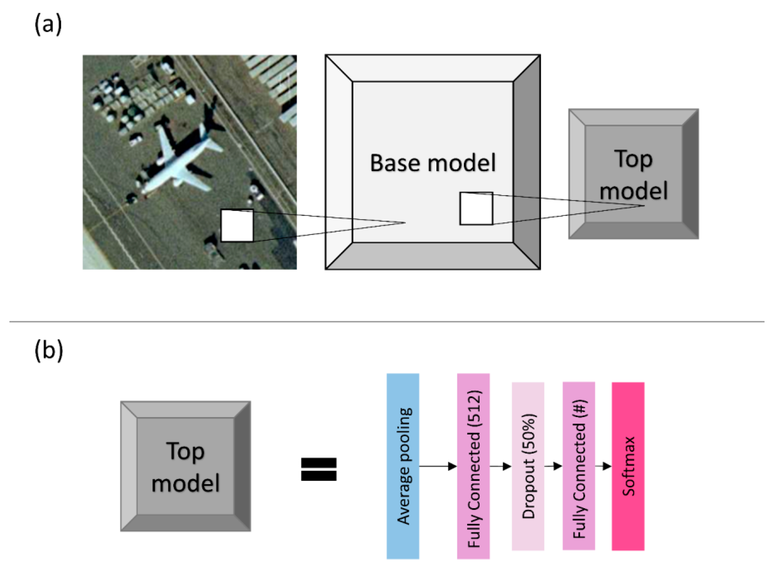
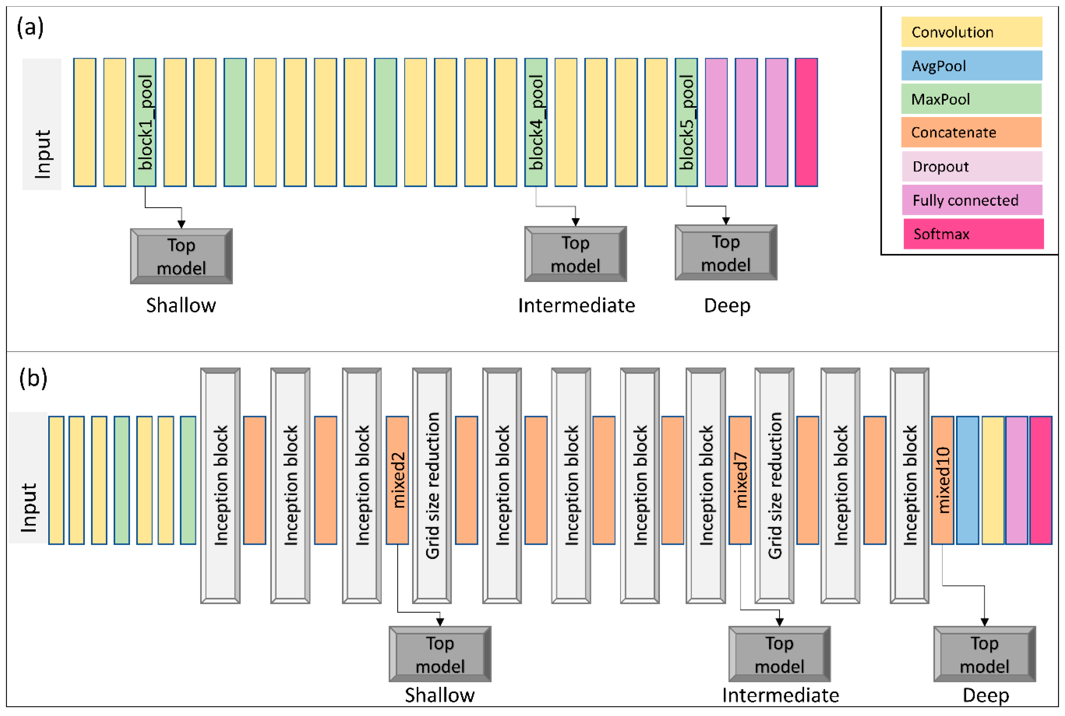
To evaluate the transfer learning process from natural images to remote sensing datasets, we use VGG19 and Inception V3 models and train a small classification network on top of such models. We refer to the original CNN model structure, part of VGG19 or part of Inception V3, as the “base model”, and the small classification network as the “top model” (Figure 1). The top model is composed of an average pooling, followed by one fully connected layer with 512 neurons, a dropout layer [59] used during training, and a final fully connected layer with a softmax output where the number of neurons is dependent on the number of classes for the task (i.e., 21 for UCMerced, 30 for AID, 38 for PatternNet). The dropout is a simple technique useful to avoid overfitting in which random connections are disabled during training. Note the top model will be specific to the secondary task and for each one of the datasets, whereas the base model, when containing the weights learned during training for the primary task, will have its layers presenting the transition from general to specific features. The models we used were primarily trained on the ImageNet dataset and are available online (e.g., through Keras or TensorFlow websites). We evaluate how dependent the transfer learning process is on the transition from general to specific features by extracting features in three different positions for each one of the retrained models and we denominate them “shallow”, “intermediate”, and “deep” (Figure 2). The shallow experiment uses the initial blocks of the base models to extract features and adds the top model. The intermediate experiment extracts the block somewhere in the middle of the base model. Finally, the deep experiment uses all the blocks of the original base model, except the original final classification layers.

5.2. Stochastic Gradient Descent versus Adaptive Optimization Methods

In the search for the global minima, optimization algorithms frequently use the gradient descent strategy. To compute the gradient of the loss function, we sum the error of each sample. Using our PatternNet data split as example, we first loop through all training set containing 21,280 samples before updating the gradient. Therefore, to move a single step towards the minima, we compute the error 21,280 times. A common approach to avoid computing the error for all training samples before moving a step is to use stochastic gradient descent (SGD).

The SGD uses a straightforward approach; instead of using the sum of all training errors (the loss), SGD uses the error gradient of a single sample at each iteration. Bottou [60] observed that SGD show good performance for large-scale problems. SGD is the building block used by many optimization algorithms that apply some variation to achieve better convergence rates (e.g., [61,62]). Kingma and Ba [63] observed that SGD has a great practical importance in many fields of science and engineering and propose Adam, a method for efficient stochastic optimization. Ruder [64] recommends using Adam as the best overall optimization choice.

However, Wilson et al. [65] reported that the solutions found by adaptive methods (such as Adam) have a worse generalization than SGD, even though solutions found by adaptive optimization methods have a better performance on the training set. Our optimization experiment is straightforward: we compare the training, validation losses and the test accuracy for the UCMerced dataset using different optimization methods: SGD, Adam, and Adamax, a variant of Adam that makes use of the infinity norm, also described by Kingma and Ba [63]. We perform such analysis using the shallow-intermediate-deep VGG19 and shallow-intermediate-deep Inception V3 to fit the UCMerced dataset starting the models with randomly initialized weights.

5.3. General to Specific Layer Transition of CNN Models

As mentioned above, many CNN models trained on natural images show a very common characteristic. Layers closer to the input data tend to learn general features, then there is a transition to more specific dataset features. For example, a CNN trained to classify the 21 UCMerced dataset has in its final layer 21 softmax outputs, with each output specifically identifying one of the 21 classes. Therefore, the final layer in this example is very specific for the UCMerced task; the final layer receives a set of features coming from the previous layers and outputs a set of probabilities accounting for the 21 UCMerced classes. These are intuitive notions of general vs. specific features that are sufficient for the experiments to be performed. Yosinski et al. [24] provide a rigorous definition of general and specific features.

To observe how the transition from general to specific features can affect the transfer learning process of remote-sensing datasets, we use the shallow, intermediate, and deep VGG19 and Inception V3 described in Section 5.1. Three training modes are performed: feature extraction, fine tuning, and randomly initialized weights. Feature extraction “locks” (or “freezes”) the pre-trained layers extracted from the base models. Fine tuning starts as feature extraction, with the base model frozen, but eventually allows all the layers of the model to learn. The randomly initialized weights mode starts the entire model with randomly initialized weights after which all the weights are updated during training. Randomly initialized weights is the ordinary CNN training, not a transfer learning process. For the sake of standardization, all modes train the model for 100 epochs. In fine tuning, the first step (part of the model is frozen) is trained for 50 epochs, and the second step (all layers of the model are free to learn) for another 50 epochs.

6. Results

6.1. Stochastic Gradient Descent versus Adaptive Optimization Methods

We train the shallow, intermediate, and deep VGG19 and Inception V3 models using the UCMerced dataset with different optimizers.

Table 5. Naming convention and optimizer details.

Name	Optimizer Details
Stochastic gradient descent, SGD (1e-2)	SGD optimizer with learning rate of 0.01
SGD (1e-2) momentum 0.9	SGD optimizer with learning rate of 0.01 and momentum 0.9
SGD (1e-3)	SGD optimizer with learning rate of 0.001
SGD (1e-3) momentum 0.9	SGD optimizer with learning rate of 0.001 and momentum 0.9
Adam (1e-2)	Adam optimizer with learning rate of 0.01 and default parameters as described in [51]
Adamax (2e-3)	Adamax optimizer with learning rate of 0.02 and default parameters as described in [51]

Note: Numbers in parenthesis on left column are used as reference to reference learning rate values.

shows the naming convention we use here. Figure 3 shows the accuracy per epoch for each one of the trained models, with each one of the optimizers. Figure 4 shows the accuracy on the test set obtained by each one of the models, with each one of the optimizers. Figure 5 shows the difference in accuracy between the training set and the test set.

Table 6. Optimizer performance summary.

Optimizer	Average Accuracy	Median Accuracy
SGD (1e-2)	0.82	0.80
SGD (1e-2) momentum 0.9	0.53	0.66
SGD (1e-3)	0.74	0.75
SGD (1e-3) momentum 0.9	0.81	0.82
Adam (1e-2)	0.59	0.81
Adamax (2e-3)	0.59	0.85

Note: Highest values in each column are highlighted in bold.

shows a summary of optimizer performance on the test set with the computation of a simple average and median of the accuracy across all tests performed. This test was run using a batch size of 16 on a NVIDIA Quadro M2000.

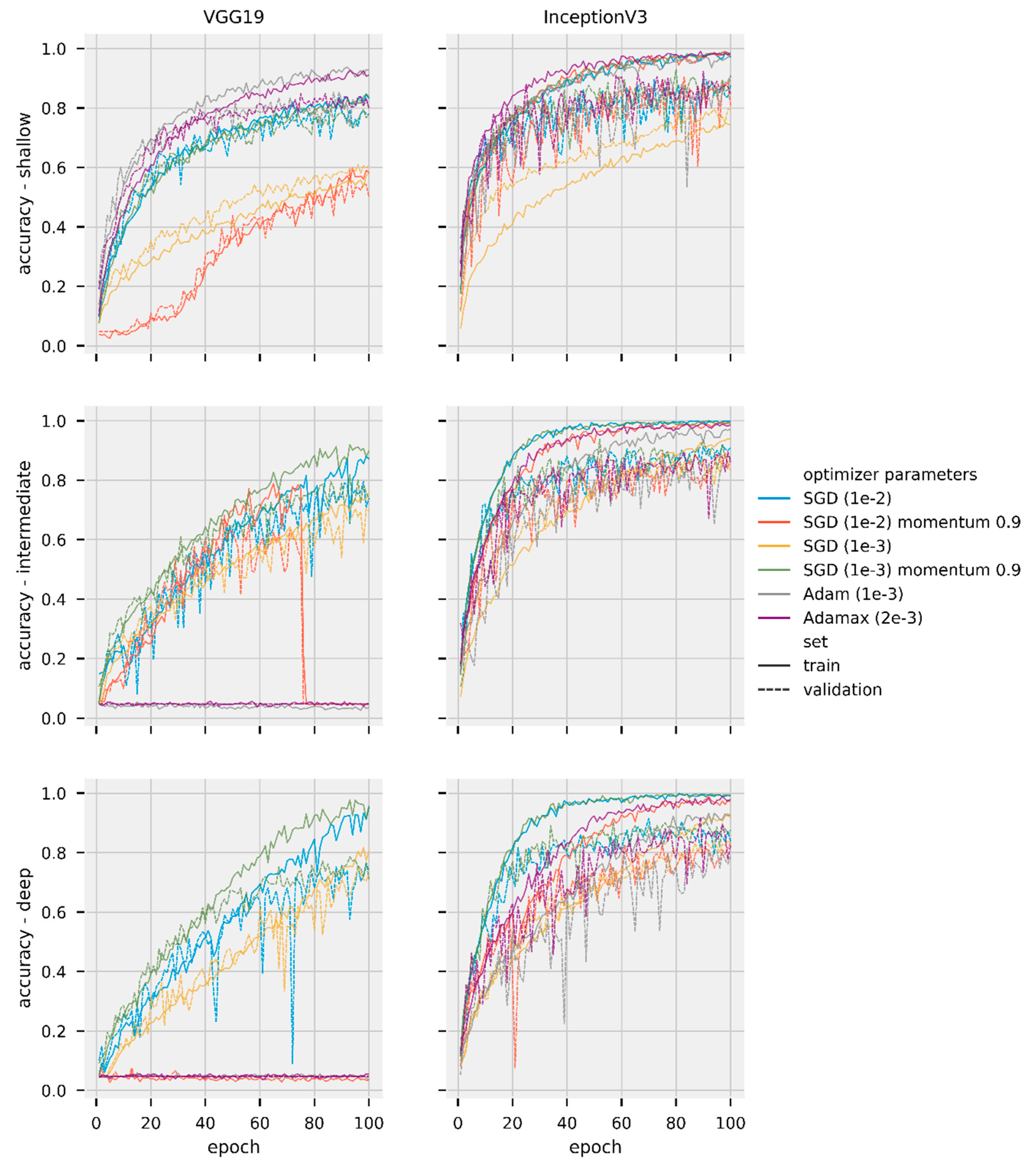
Figure 3 shows a different performance for all the optimizers used. For example, the VGG19 deep accuracy indicates the model was still improving after 100 epochs for many of the optimizers used, e.g., SGD (1e-3). Figure 3 also shows that some combinations of model and optimizer became stuck in a local minimum—e.g., Adam (1e-3), Adamax (2e-3)—and did not improve their performance.

Discarding the combinations of model and optimizer stuck in local minima, Figure 4 shows that, in general, the models achieve a comparable performance after 100 epochs. Figure 5 provides a more detailed comparison of the difference of model performance in the training and test sets. Figure 5 also presents some cases in which the accuracy in the test set was higher than the in the training set, e.g., SGD (1e-3) for Inception V3 shallow model. Validation and test set metrics better than training set metrics can be caused by the dropout layer, as during training less information is available for the model, or simply because of the data split; the training set is generally larger than validation and test sets and can incorporate a higher complexity in its samples.

Unlike the poor generalization performance of adaptive methods compared to SGD optimizers reported by Wilson et al. [65], our results do not find significant differences in performance for the optimizers tested. In fact, results in Figure 5 indicate that for our task SGDs had a slightly worse performance. SGD (1e-3) momentum 0.9 and SGD (1e-2) had the larger difference between accuracy in training and test set for VGG19 intermediate and deep models. SGD (1e-2) momentum 0.9 had the worst performance for Inception V3 shallow.

6.2. General to Specific Layer Transition of CNN Models

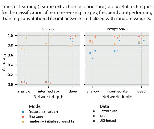
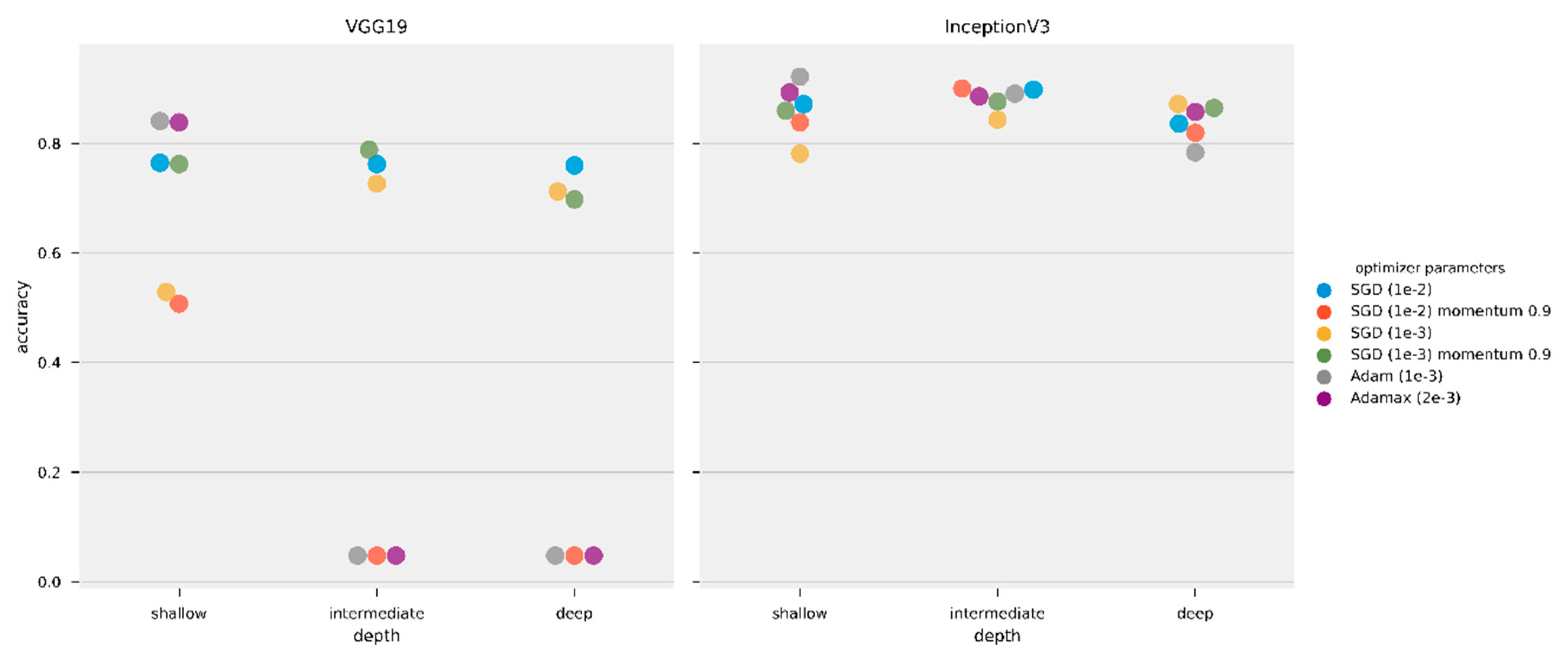
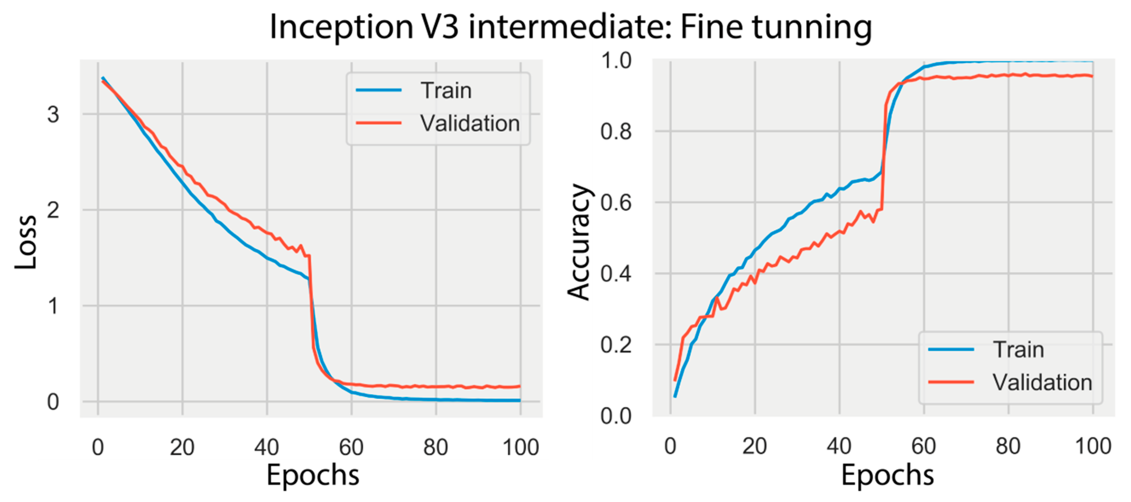
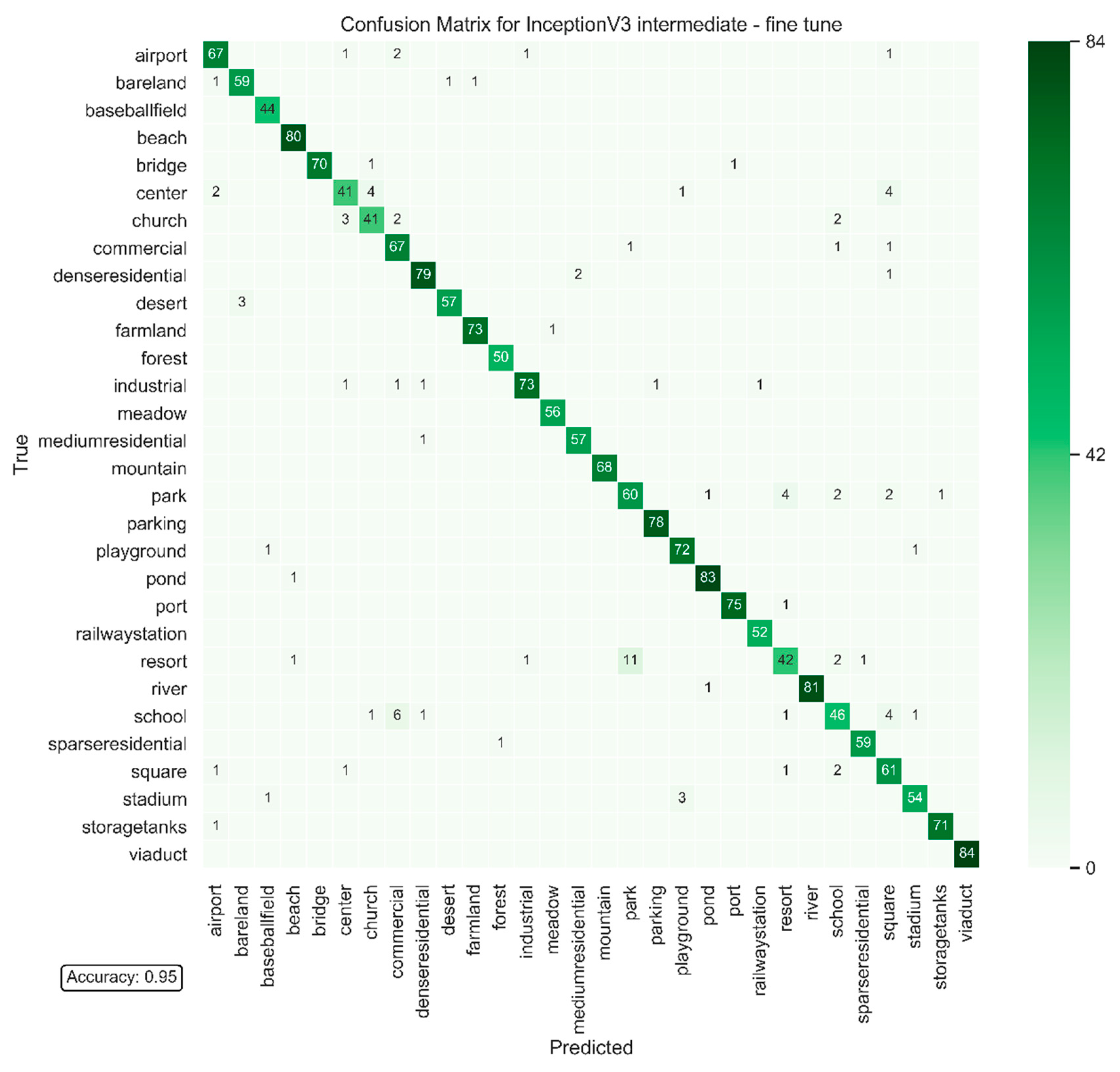
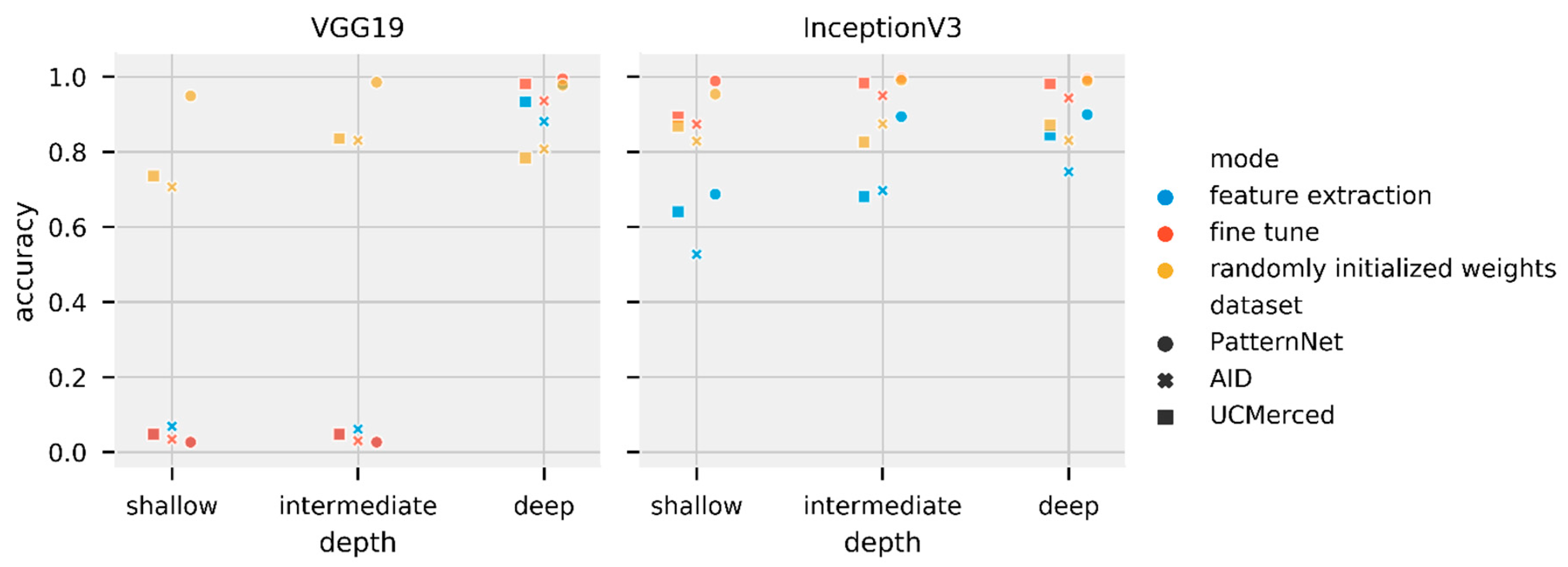
This section shows the results of transfer learning, both feature extraction and fine-tuning modes, as well as training the models with randomly initialized weights.

Table 7. Best test set accuracy for Inception V3 and VGG19 version for each dataset using SGD (1e-3) momentum 0.9 optimizer.

Dataset	Model	Depth	Mode	Accuracy
PatternNet	Inception V3	intermediate	fine tune	0.997
	VGG19	deep	fine tune	0.995
AID	Inception V3	intermediate	fine tune	0.950
	VGG19	deep	fine tune	0.936
UCMerced	Inception V3	intermediate	fine tune	0.983
	VGG19	deep	fine tune	0.981

Note: The best performing model for each dataset is highlighted in bold.

shows a summary of the best performance of Inception V3 and VGG19 trained using SGD (1e-3) momentum 0.9. We chose SGD (1e-3) momentum 0.9 as it is the optimizer with the second-best median in Table 6, and did not become stuck in local minima. The table shows, for each dataset and each model, which depth and training mode achieved the highest accuracy in the test set. We select AID trained on Inception V3 intermediate, one out of the 54 experiments (three datasets, two models, three depths, three training modes), to provide more details of the training loss-accuracy and the confusion matrix computed for the test set. Figure 6 shows the training and validation loss and accuracy through the training epochs. Figure 7 shows the correspondent confusion matrix computed on the AID test set.

The graphs in Figure 6 show a significant improvement in the performance of the model after epoch 50, when the model enters the second stage of fine tuning. After 50 epochs, the base model is unfrozen, thus all layers can learn.

Figure 8 shows an overview of the complete experiment on the test set. This figure shows the test set accuracy for all the datasets, for all the models’ depths and training modes. This test was run on a NVIDIA GeForce RTX 2060 and it took roughly six days to complete. Training of VGG shallow, intermediate, and deep with PatternNet data took roughly 4:10, 6:20, and 6:50 hours to complete. Training of InceptionV3 shallow, intermediate, and deep with PatternNet data took roughly 3:50, 5:40, and 6:50 hours to complete, respectively. These execution times are provided as simple general reference and lack more detailed analysis of performance—the computer was not entirely dedicated to experiments, thus speed might have been affected.

Our choice of optimizer, SGD (1e-3) momentum 0.9, for the transfer learning experiments was mainly based on its performance in the optimizer tests. However, Figure 8 shows that some models were still trapped in local minima, showing the optimizer was unable to improve some of the models’ performance.

Next we selected all the six models trained on PatternNet with randomly initialized weights and perform transfer learning, using the same methodology as before. Thus, we first trained CNN models on PatternNet and then applied transfer learning to train on AID and UCMerced. Note this is slightly different than the transfer learning performed before, where we split a single model in three different parts. Here we used the model in its original form (shallow, intermediate, or deep). Loss decays and confusion matrix figures, as well as the complete table with all test accuracies are provided in the supplemental materials.

Table 8. Best test set accuracy for Inception V3 and VGG19 version for each Dataset using SGD (1e-3) momentum 0.9 optimizer to perform transfer learning on models initially trained on PatternNet.

Dataset	Model	Depth	Mode	Accuracy
AID	InceptionV3	Deep	fine tune	0.838
	VGG19	intermediate	fine tune	0.833
UCMerced	InceptionV3	intermediate	fine tune	0.948
	VGG19	Deep	fine tune	0.886

Note: The best performing model for each dataset is highlighted in bold.

shows the best performing Inception V3 and VGG19 for each one of the datasets.

Finally, we repeated transfer learning tests with Adamax (2e-3), the optimizer with best median performance in Table 6, although falling in local minima in some tests.

Table 9. Best test set accuracy for Inception V3 and VGG19 version for each Dataset using Adamax (2e-3) optimizer.

Dataset	Model	Depth	Mode	Accuracy
PatternNet	InceptionV3	intermediate	fine tune	0.993
	VGG19	Deep	feature extraction	0.983
AID	InceptionV3	intermediate	fine tune	0.941
	VGG19	Deep	feature extraction	0.889
UCMerced	InceptionV3	Deep	fine tune	0.910
	VGG19	Deep	feature extraction	0.943

Note: The best performing model for each dataset is highlighted in bold.

shows a summary of the best performing Inception V3 and VGG19 trained using Adamax (2e-3) for the three datasets used. Figure 9 shows an overview of the complete experiment on the test set. We did not repeat the PatternNet to AID-UCMerced transfer learning using Adamax (2e-3) as results in Table 7 are generally better than results in Table 9.

Even though we selected SGD (1e-3) momentum 0.9 as the optimizer for the transfer learning experiments due to its performance on the optimizer tests, some models still fell into local minima. This failure shows how the choice of hyperparameters can strongly affect the performance of deep-learning models. Neither training from random initial weights (Figure 4) nor transfer learning techniques (Figure 8 and Figure 9) are exempt from the possibility of a poor performance if suboptimal hyperparameters are used. More than a marginal increase in performance, the results show that the models can completely fail when used with inappropriate hyperparameters, even if the task is appropriate for the model.

7. Discussion

Using ImageNet data, Yosinski et al. [24] found that transfer learning, even when applied to a secondary task not similar to the primary task, perform better than training CNN models with randomly initialized weights. Using medical image data, Tajbakhsh et al. [66] found that fine-tuning achieved results comparable to or better than results from training a CNN model with randomly initialized weights. Our results align with their findings. Both Figure 8 and Table 7 show the fine-tuning mode of training outperforming randomly initialized weights when using SGD (1e-3) momentum 0.9. Results in Figure 9 and Table 9 show that transfer learning performs best with the Adamax (2e-3) optimizer. However, it seems that the step size (2e-3) is too large for fine tuning in the VGG19 model, such that the VGG19 intermediate and deep models trained on fine tune and randomly initialized weights modes fall in local minima. The primary task (ImageNet, composed of natural images) is not very similar to the secondary task (remote-sensing scene classification). While there is a similarity in primary and secondary tasks datasets, such as the number of channels (red-green-blue components), images are from the visible spectra, and some objects might be present in both tasks (e.g., airplanes), the tasks are fundamentally different. Figure 5, however, shows how feature extraction can be limited by the difference in tasks. When the initial layers are frozen, the model cannot properly learn and the model starts to overfit. With the layers unfrozen, the overfitting reduces and accuracy increase. We observed a similar behavior for most of fine-tuning tests (all of the loss and accuracy per epoch can be accessed in the supplemental materials). Despite feature extraction limitations, the results show that transfer learning is an effective deep-learning approach that should not be discarded if the secondary task is not similar to the primary task. In fact, Table 8 presents striking results. Fine-tuned models initially trained on PatternNet underperformed fine tuned models trained on ImageNet. Perhaps the first explanation for such underperformance would be that the models are overfitting the PatternNet dataset. However, PatternNet models performed well on the PatternNet test set, which indicates they are not overfitting the training data. We hypothesize that the weaker performance is due to the complexity of the datasets. PatternNet is a dataset created with the objective to provide researchers with clear examples of different remote sensing scenes, whereas the ImageNet is a complex dataset where the intra-class variance, i.e. how a single class contains very different samples, is very high. As observed by Cheng et al. [3] many remote-sensing scene classification datasets have a lack of intraclass sample variations and diversity. These limitations severely limit the development of new approaches especially deep learning-based methods. Thus, CNN models trained on the ImageNet need to develop more generic, perhaps robust, filters to be able to identify ImageNet’s classes properly.

8. Conclusions

Our objective with this paper was to investigate the use of transfer learning in the analysis of remote-sensing data, as well as how the CNN performance depends on the depth of the network and on the amount of training data available. Our experiments, based on three distinct remote-sensing datasets and two popular CNN models, show that transfer learning, specifically fine tuning CNNs is a powerful tool for remote-sensing scene classification. Much like the findings in other experiments, the results we found show that transfer from natural images (ImageNet) to remote-sensing imagery is possible. Despite the relatively large difference between primary and secondary tasks, transfer learning training mode generally outperformed training a CNN with randomly initialized weights and achieved the best results overall. Curiously, fine-tuning models primarily trained on the generic ImageNet dataset overperformed fine-tuning models primarily trained on PatternNet dataset. As expected, our results also indicate that for a particular application, the amount of training data available plays a significant role on the performance of the CNN models. In general we observed a larger accuracy difference between transfer learning and training with randomly initialized weights using the smaller UCMerced dataset, whereas accuracy differences were smaller when using the larger PatternNet dataset. Model robustness was also clear on the results. In several instances the VGG19 ended up stuck on local minima, both during optimization testing and during transfer learning testing. The VGG19 shallow and intermediate models’ results exhibit a performance degradation caused by splitting the primary trained CNN model between co-adapted neurons on neighboring layers. VGG19 shallow and intermediate on randomly initialized mode, however, performed satisfactorily. In spite of our simplistic model split without detailed attention to co-adaption of neurons between layers, Inception V3 passed all experiments without falling into local minima.

The results seem to corroborate that feature extraction or fine-tuning well-established CNN models offer a practical way to achieve the best performance for remote-sensing scene classification. Although fine-tuning the originally more complex deep models might present satisfactory results, splitting the original model can perhaps improve performance. Note, the fine-tuning Inception V3 intermediate model outperformed Inception V3 deep model. With datasets large enough, randomly initialized weights are also an appropriate choice for training. However, it is often hard to know when a dataset is large enough. Our recommendation is to start from the deep models and try to reduce model’s size as it is easier to overfit models with too many weights.

References

- Emery, W.; Camps, A. Chapter 1—The History of Satellite Remote Sensing. In Introduction to Satellite Remote Sensing; Emery, W., Camps, A., Eds.; Elsevier: Amsterdam, The Netherlands, 2017; pp. 1–42. [Google Scholar] [CrossRef]
- Zhou, W.; Newsam, S.; Li, C.; Shao, Z. PatternNet: A benchmark dataset for performance evaluation of remote sensing image retrieval. ISPRS J. Photogramm. Remote Sens. 2018, 145, 197–209. [Google Scholar] [CrossRef] [Green Version]
- Cheng, G.; Han, J.; Lu, X. Remote Sensing Image Scene Classification: Benchmark and State of the Art. Proc. IEEE 2017, 105, 1865–1883. [Google Scholar] [CrossRef] [Green Version]
- Xiao, Y.; Zhan, Q. A review of remote sensing applications in urban planning and management in China. In Proceedings of the 2009 Joint Urban Remote Sensing Event, Shanghai, China, 20–22 May 2009; pp. 1–5. [Google Scholar] [CrossRef]
- Skidmore, A.K.; Bijker, W.; Schmidt, K.; Kumar, L. Use of remote sensing and GIS for sustainable land management. ITC J. 1997, 3, 302–315. [Google Scholar]
- Lentile, L.B.; Holden, Z.A.; Smith, A.M.; Falkowski, M.J.; Hudak, A.T.; Morgan, P.; Lewis, S.A.; Gessler, P.E.; Benson, N.C. Remote sensing techniques to assess active fire characteristics and post-fire effects. Int. J. Wildl. Fire 2006, 15, 319–345. [Google Scholar] [CrossRef]
- Daldegan, G.A.; Roberts, D.A.; Ribeiro, F.D. Spectral mixture analysis in Google Earth Engine to model and delineate fire scars over a large extent and a long time-series in a rainforest-savanna transition zone. Remote Sens. Environ. 2019, 232. [Google Scholar] [CrossRef]
- Sebai, H.; Kourgli, A.; Serir, A. Dual-tree complex wavelet transform applied on color descriptors for remote-sensed images retrieval. J. Appl. Remote Sens. 2015, 9. [Google Scholar] [CrossRef]
- Bosilj, P.; Aptoula, E.; Lefèvre, S.; Kijak, E. Retrieval of Remote Sensing Images with Pattern Spectra Descriptors. ISPRS Int. J. Geo-Inf. 2016, 5, 228. [Google Scholar] [CrossRef] [Green Version]
- Shao, Z.; Zhou, W.; Zhang, L.; Hou, J. Improved color texture descriptors for remote sensing image retrieval. J. Appl. Remote Sens. 2014, 8. [Google Scholar] [CrossRef] [Green Version]
- Scott, G.J.; Klaric, M.N.; Davis, C.H.; Shyu, C.-R. Entropy-Balanced Bitmap Tree for Shape-Based Object Retrieval from Large-Scale Satellite Imagery Databases. IEEE Trans. Geosci. Remote Sens. 2011, 49, 1603–1616. [Google Scholar] [CrossRef]
- Lowe, D.G. Distinctive Image Features from Scale-Invariant Keypoints. Int. J. Comput. Vis. 2004, 60, 91–110. [Google Scholar] [CrossRef]
- Hu, F.; Xia, G.-S.; Hu, J.; Zhang, L. Transferring Deep Convolutional Neural Networks for the Scene Classification of High-Resolution Remote Sensing Imagery. Remote Sens. 2015, 7, 14680–14707. [Google Scholar] [CrossRef] [Green Version]
- Yang, X.; Ye, Y.; Li, X.; Lau, R.Y.K.; Zhang, X.; Huang, X. Hyperspectral Image Classification with Deep Learning Models. IEEE Trans. Geosci. Remote Sens. 2018, 56, 5408–5423. [Google Scholar] [CrossRef]
- Le Cun, Y.; Bengio, Y.; Hinton, G. Deep learning. Nature 2015, 521, 436–444. [Google Scholar] [CrossRef] [PubMed]
- Krizhevsky, A.; Sutskever, I.; Hinton, G.E. ImageNet Classification with Deep Convolutional Neural Networks. In Proceedings of the 25th International Conference on Neural Information Processing Systems, Lake Tahoe, NV, USA, 3–6 December 2012; Volume 1, pp. 1097–1105. [Google Scholar]
- Le Cun, Y. The MNIST Database of Handwritten Digits. 1998. Available online: http://yann.lecun.com/exdb/mnist/ (accessed on 15 November 2019).
- Russakovsky, O.; Deng, J.; Su, H.; Krause, J.; Satheesh, S.; Ma, S.; Huang, Z.; Karpathy, A.; Khosla, A.; Bernstein, M.; et al. ImageNet Large Scale Visual Recognition Challenge. Int. J. Comput. Vis. 2015, 115, 211–252. [Google Scholar] [CrossRef] [Green Version]
- Huang, G.; Sun, Y.; Liu, Z.; Sedra, D.; Weinberger, K. Deep Networks with Stochastic Depth. In Proceedings of the 14th European Conference, Amsterdam, The Netherlands, 11–14 October 2016. [Google Scholar]
- Simonyan, K.; Vedaldi, A.; Zisserman, A. Deep Inside Convolutional Networks: Visualising Image Classification Models and Saliency Maps. arXiv 2013, arXiv:1312.6034. [Google Scholar]
- Yin, X.; Chen, W.; Wu, X.; Yue, H. Fine-tuning and visualization of convolutional neural networks. In Proceedings of the 2017 12th IEEE Conference on Industrial Electronics and Applications (ICIEA), Siem Reap, Cambodia, 18–20 June 2017; pp. 1310–1315. [Google Scholar] [CrossRef]
- Olah, C.; Mordvintsev, A.; Schubert, L. Feature Visualization. Distill 2017. [Google Scholar] [CrossRef]
- Olah, C.; Satyanarayan, A.; Johnson, I.; Carter, S.; Schubert, L.; Ye, K.; Mordvintsev, A. The Building Blocks of Interpretability. Distill 2018. [Google Scholar] [CrossRef]
- Yosinski, J.; Clune, J.; Bengio, Y.; Lipson, H. How transferable are features in deep neural networks? In Proceedings of the 27th International Conference on Neural Information Processing Systems, Montreal, QC, Canada, 8–13 December 2014; Volume 27, pp. 3320–3328. [Google Scholar]
- Caruana, R. Learning Many Related Tasks at the Same Time with Backpropagation. In Advances in Neural Information Processing Systems 7; Tesauro, G., Touretzky, D.S., Leen, T.K., Eds.; MIT Press: Cambridge, MA, USA, 1995; pp. 657–664. [Google Scholar]
- Bengio, Y. Deep Learning of Representations for Unsupervised and Transfer Learning. In Proceedings of the ICML Workshop on Unsupervised and Transfer Learning, Scotland, UK, 26 June–1 July 2012; Volume 27, pp. 17–36. [Google Scholar]
- Carranza-Rojas, J.; Goeau, H.; Bonnet, P.; Mata-Montero, E.; Joly, A. Going deeper in the automated identification of Herbarium specimens. BMC Evol. Biol. 2017, 17, 181. [Google Scholar] [CrossRef] [Green Version]
- Esteva, A.; Kuprel, B.; Novoa, R.A.; Ko, J.; Swetter, S.M.; Blau, H.M.; Thrun, S. Dermatologist-level classification of skin cancer with deep neural networks. Nature 2017, 542, 115–118. [Google Scholar] [CrossRef]
- De Lima, R.P.; Suriamin, F.; Marfurt, K.J.; Pranter, M.J. Convolutional neural networks as aid in core lithofacies classification. Interpretation 2019, 7, SF27–SF40. [Google Scholar] [CrossRef]
- Duarte-Coronado, D.; Tellez-Rodriguez, J.; de Lima, R.P.; Marfurt, K.; Slatt, R. Deep convolutional neural networks as an estimator of porosity in thin-section images for unconventional reservoirs. In SEG Technical Program Expanded Abstracts 2019; SEG: San Antonio, TX, USA, 15–20 September 2019; pp. 3181–3184. [Google Scholar] [CrossRef]
- De Lima, R.P.; Marfurt, K.; Duarte, D.; Bonar, A. Progress and Challenges in Deep Learning Analysis of Geoscience Images. In Proceedings of the 81st EAGE Conference and Exhibition 2019, London, UK, 3–6 June 2019. [Google Scholar] [CrossRef]
- De Lima, R.P.; Bonar, A.; Coronado, D.D.; Marfurt, K.; Nicholson, C. Deep convolutional neural networks as a geological image classification tool. Sediment. Rec. 2019, 17, 4–9. [Google Scholar] [CrossRef]
- Minaee, S.; Abdolrashidi, A.; Su, H.; Bennamoun, M.; Zhang, D. Biometric Recognition Using Deep Learning: A Survey. arXiv 2019, arXiv:1912.00271. [Google Scholar]
- Razavian, A.S.; Azizpour, H.; Sullivan, J.; Carlsson, S. CNN Features Off-the-Shelf: An Astounding Baseline for Recognition. In Proceedings of the 2014 IEEE Conference on Computer Vision and Pattern Recognition Workshops, Columbus, OH, USA, 23–28 June 2014; pp. 512–519. [Google Scholar] [CrossRef] [Green Version]
- Chen, Z.; Zhang, T.; Ouyang, C.; Chen, Z.; Zhang, T.; Ouyang, C. End-to-End Airplane Detection Using Transfer Learning in Remote Sensing Images. Remote Sens. 2018, 10, 139. [Google Scholar] [CrossRef] [Green Version]
- Rostami, M.; Kolouri, S.; Eaton, E.; Kim, K. Deep Transfer Learning for Few-Shot SAR Image Classification. Remote Sens. 2019, 11, 1374. [Google Scholar] [CrossRef] [Green Version]
- Weinstein, B.G.; Marconi, S.; Bohlman, S.; Zare, A.; White, E. Individual Tree-Crown Detection in RGB Imagery Using Semi-Supervised Deep Learning Neural Networks. Remote Sens. 2019, 11, 1309. [Google Scholar] [CrossRef] [Green Version]
- Huot, F.; Biondi, B.; Beroza, G. Jump-starting neural network training for seismic problems. In SEG Technical Program Expanded Abstracts 2018; SEG: Anaheim, CA, USA, 14–19 October 2018; pp. 2191–2195. [Google Scholar] [CrossRef]
- De Lima, R.P.; Lin, Y.; Marfurt, K.J. Transforming seismic data into pseudo-RGB images to predict CO2 leakage using pre-learned convolutional neural networks weights. In SEG Technical Program Expanded Abstracts 2019; SEG: San Antonio, TX, USA, 15–20 September 2019; pp. 2368–2372. [Google Scholar] [CrossRef]
- Simonyan, K.; Zisserman, A. Very Deep Convolutional Networks for Large-Scale Image Recognition. arXiv 2014, arXiv:1409.1556. [Google Scholar]
- Szegedy, C.; Vanhoucke, V.; Ioffe, S.; Shlens, J.; Wojna, Z. Rethinking the Inception Architecture for Computer Vision. In Proceedings of the IEEE Conference on Computer Vision and Pattern Recognition, Las Vegas, NV, USA, 27–30 June 2016. [Google Scholar]
- Google. Machine Learning Glossary. 2019. Available online: https://developers.google.com/machine-learning/glossary/ (accessed on 3 November 2019).
- Yang, Y.; Newsam, S. Bag-of-visual-words and spatial extensions for land-use classification. In Proceedings of the 18th SIGSPATIAL International Conference on Advances in Geographic Information Systems—GIS’10, San Jose, CA, USA, 3–5 November 2010; p. 270. [Google Scholar] [CrossRef]
- Xia, G.S.; Hu, J.; Hu, F.; Shi, B.; Bai, X.; Zhong, Y.; Zhang, L.; Lu, X. AID: A Benchmark Data Set for Performance Evaluation of Aerial Scene Classification. IEEE Trans. Geosci. Remote Sens. 2017, 55, 3965–3981. [Google Scholar] [CrossRef] [Green Version]
- Springenberg, J.T.; Dosovitskiy, A.; Brox, T.; Riedmiller, M. Striving for Simplicity: The All Convolutional Net. arXiv 2014, arXiv:1412.6806. [Google Scholar]
- Dumoulin, V.; Visin, F. A guide to convolution arithmetic for deep learning. arXiv 2016, arXiv:1603.07285. [Google Scholar]
- Szegedy, C.; Liu, W.; Jia, Y.; Sermanet, P.; Reed, S.; Anguelov, D.; Erhan, D.; Vanhoucke, V.; Rabinovich, A. Going Deeper with Convolutions. In Proceedings of the IEEE Conference on Computer Vision and Pattern Recognition, Boston, MA, USA, 7–12 June 2015. [Google Scholar]
- Sandler, M.; Howard, A.; Zhu, M.; Zhmoginov, A.; Chen, L.-C. MobileNetV2: Inverted Residuals and Linear Bottlenecks. arXiv 2018, arXiv:1801.04381. [Google Scholar]
- He, K.; Zhang, X.; Ren, S.; Sun, J. Identity Mappings in Deep Residual Networks. In Proceedings of the Computer Vision—ECCV 2016, Amsterdam, The Netherlands, 8–16 October 2016; pp. 630–645. [Google Scholar]
- Huang, G.; Liu, Z.; Weinberger, K.Q. Densely Connected Convolutional Networks. In Proceedings of the IEEE Conference on Computer Vision and Pattern Recognition, Honolulu, HI, USA, 21–26 July 2017. [Google Scholar]
- Zoph, B.; Vasudevan, V.; Shlens, J.; Le, Q.V. Learning Transferable Architectures for Scalable Image Recognition. In Proceedings of the IEEE Conference on Computer Vision and Pattern Recognition, Salt Lake City, UT, USA, 18–22 June 2018. [Google Scholar]
- Chollet, F. Xception: Deep Learning with Depthwise Separable Convolutions. In Proceedings of the IEEE Conference on Computer Vision and Pattern Recognition, Honolulu, HI, USA, 21–26 July 2017. [Google Scholar]
- Vaswani, A.; Shazeer, N.; Parmar, N.; Uszkoreit, J.; Jones, L.; Gomez, A.N.; Kaiser, Ł.; Polosukhin, I. Attention is all you need. In Advances in Neural Information Processing Systems; MIT Press: Long Beach, CA, USA, 2017; pp. 5998–6008. [Google Scholar]
- Wang, J.; Shen, L.; Qiao, W.; Dai, Y.; Li, Z. Deep Feature Fusion with Integration of Residual Connection and Attention Model for Classification of VHR Remote Sensing Images. Remote Sens. 2019, 11, 1617. [Google Scholar] [CrossRef] [Green Version]
- Xu, R.; Tao, Y.; Lu, Z.; Zhong, Y. Attention-Mechanism-Containing Neural Networks for High-Resolution Remote Sensing Image Classification. Remote Sens. 2018, 10, 1602. [Google Scholar] [CrossRef] [Green Version]
- Keras: The Python Deep Learning Library. Available online: https://keras.io (accessed on 15 November 2019).
- Abadi, M.; Barham, P.; Chen, J.; Chen, Z.; Davis, A.; Dean, J.; Devin, M.; Ghemawat, S.; Irving, G.; Isard, M.; et al. TensorFlow: A system for large-scale machine learning. In Proceedings of the 12th USENIX Symposium on Operating Systems Design and Implementation (OSDI 16), Savannah, GA, USA, 2–4 November 2016; pp. 265–283. [Google Scholar]
- Glorot, X.; Bengio, Y. Understanding the difficulty of training deep feedforward neural networks. In Proceedings of the International Conference on Artificial Intelligence and Statistics (AISTATS’10), Chia Laguna Resort, Sardinia, Italy, 13–15 May 2010. [Google Scholar]
- Srivastava, N.; Hinton, G.; Krizhevsky, A.; Sutskever, I.; Salakhutdinov, R. Dropout: A Simple Way to Prevent Neural Networks from Overfitting. J. Mach. Learn. Res. 2014, 15, 1929–1958. [Google Scholar]
- Bottou, L. Large-Scale Machine Learning with Stochastic Gradient Descent. In Proceedings of the COMPSTAT’2010, 19th International Conference on Computational Statistics, Paris, France, 22–27 August 2010; pp. 177–186. [Google Scholar] [CrossRef] [Green Version]
- Duchi, J.; Hazan, E.; Singer, Y. Adaptive Subgradient Methods for Online Learning and Stochastic Optimization. J. Mach. Learn. Res. 2011, 12, 2121–2159. [Google Scholar]
- Tieleman, T.; Hinton, G. Lecture 6.5—RmsProp: Divide the gradient by a running average of its recent magnitude. Neural Netw. Mach. Learn. 2012, 26–30. [Google Scholar]
- Kingma, D.P.; Ba, J. Adam: A Method for Stochastic Optimization. arXiv 2014, arXiv:1412.6980. [Google Scholar]
- Ruder, S. An overview of gradient descent optimization algorithms. arXiv 2016, arXiv:1609.04747. [Google Scholar]
- Wilson, A.C.; Roelofs, R.; Stern, M.; Srebro, N.; Recht, B. The Marginal Value of Adaptive Gradient Methods in Machine Learning. In Advances in Neural Information Processing Systems 30; Guyon, I., Luxburg, U.V., Bengio, S., Wallach, H., Fergus, R., Vishwanathan, S., Garnett, R., Eds.; Curran Associates, Inc.: Long Beach, CA, USA, 2017; pp. 4148–4158. [Google Scholar]
- Tajbakhsh, N.; Shin, J.Y.; Gurudu, S.R.; Hurst, R.T.; Kendall, C.B.; Gotway, M.B.; Liang, J. Convolutional Neural Networks for Medical Image Analysis: Full Training or Fine Tuning? IEEE Trans. Med. Imaging 2016, 35, 1299–1312. [Google Scholar] [CrossRef] [Green Version]
Figure 1.
Visualization of the models used. (a) shows a sample image from UCMerced, the base model, and the top model. (b) provides more details for the top model. The base model is dependent on the convolutional neural network (CNN) architecture used for transfer learning and it is detailed in Figure 2. Top model is the same for all experiments. Note the pound sign “#” represents the number of classes, which depends on the dataset used.
Figure 2.
Visual representation of the models used. In both panels, data flows from left to right. Both panes use the same color code for layer representation. (a) shows the VGG19 shallow, intermediate, and deep models – based on the naming convention we are using. (b) shows the Inception V3 shallow, intermediate, and deep models. For easier reference, we wrote the layer names (as implemented in Keras) for each one of the layers we used to split the original CNN models. Note for each one of the depth levels (shallow, intermediate, deep), we simple use the model up to the detour and connect it with our top model (e.g., when training VGG19 shallow, the data goes through two convolutional layers, one max pooling layers, and exits into our top model). Please refer to Simonyan and Zisserman [40] and Szegedy et al. [41] for details on VGG19 and Inception V3, respectively.
Figure 3.
Accuracy per epoch for training and validation sets for different models and optimizers trained on the UCMerced dataset. The left column shows results for VGG19 models. The right column shows results for Inception V3 models. The first row shows shallow models, center shows intermediate, bottom shows deep models. Different colors represent different optimizers. Different and line style represent different datasets (solid for training, dashed for validation).
Figure 4.
Test set accuracy obtained by the models using different optimizers training on the same UCMerced dataset. The left panel shows VGG 19 results, right panel shows Inception V3 results.
Figure 5.
Difference between training set and test set accuracy obtained by the models using different optimizers training on the same UCMerced dataset. The left panel shows VGG 19 results, right panel shows Inception V3 results. Note, as shown in Figure 4, that SGD (1e-2), Adam (1e-2), and Adamax (2e-3) results of theVGG19 intermediate and deep models remained stuck on local minima.
Figure 6.
Train and validation loss and accuracy for the Inception V3 intermediate in the fine tuning mode trained on the AID dataset using SGD (1e-3) momentum 0.9.
Figure 7.
Confusion matrix for the test set of AID dataset for the Inception V3 intermediate in the fine-tune mode using SGD (1e-3) momentum 0.9.
Figure 8.
Test set accuracy for all VGG19 and Inception V3 versions trained with all datasets using SGD (1e-3) momentum 0.9. Left panel shows VGG 19 results, right panel shows Inception V3 results. Note VGG19 shallow and intermediate feature extraction and fine-tune versions were trapped in local minima. Some of the points in local minima appear wine-colored as the blue (feature extraction) points and red (fine tune) points are very closed and partially overlaying each other.
Figure 9.
Test set accuracy for all VGG19 and Inception V3 versions trained with all datasets using Adamax (2e-3). Left panel shows VGG 19 results, right panel shows Inception V3 results. Note VGG19 shallow and intermediate feature extraction and fine tuning versions were trapped in local minima.