Article

Multi-Temporal Unmanned Aerial Vehicle Remote Sensing for Vegetable Mapping Using an Attention-Based Recurrent Convolutional Neural Network

1
College of Resources and Environmental Sciences, China Agricultural University, Beijing 100193, China
2
College of Land Science and Technology, China Agricultural University, Beijing 100083, China
3
School of Surveying and Geo-Informatics, Shandong Jianzhu University, Jinan 250101, China
*
Author to whom correspondence should be addressed.
Remote Sens. 2020, 12(10), 1668; https://0-doi-org.brum.beds.ac.uk/10.3390/rs12101668
Submission received: 19 April 2020 / Revised: 18 May 2020 / Accepted: 21 May 2020 / Published: 22 May 2020
(This article belongs to the Special Issue UAS-Remote Sensing Methods for Mapping, Monitoring and Modeling Crops)

Abstract

:
Vegetable mapping from remote sensing imagery is important for precision agricultural activities such as automated pesticide spraying. Multi-temporal unmanned aerial vehicle (UAV) data has the merits of both very high spatial resolution and useful phenological information, which shows great potential for accurate vegetable classification, especially under complex and fragmented agricultural landscapes. In this study, an attention-based recurrent convolutional neural network (ARCNN) has been proposed for accurate vegetable mapping from multi-temporal UAV red-green-blue (RGB) imagery. The proposed model firstly utilizes a multi-scale deformable CNN to learn and extract rich spatial features from UAV data. Afterwards, the extracted features are fed into an attention-based recurrent neural network (RNN), from which the sequential dependency between multi-temporal features could be established. Finally, the aggregated spatial-temporal features are used to predict the vegetable category. Experimental results show that the proposed ARCNN yields a high performance with an overall accuracy of 92.80%. When compared with mono-temporal classification, the incorporation of multi-temporal UAV imagery could significantly boost the accuracy by 24.49% on average, which justifies the hypothesis that the low spectral resolution of RGB imagery could be compensated by the inclusion of multi-temporal observations. In addition, the attention-based RNN in this study outperforms other feature fusion methods such as feature-stacking. The deformable convolution operation also yields higher classification accuracy than that of a standard convolution unit. Results demonstrate that the ARCNN could provide an effective way for extracting and aggregating discriminative spatial-temporal features for vegetable mapping from multi-temporal UAV RGB imagery.

Graphical Abstract

1. Introduction

Accurate vegetable mapping is of great significance for modern precision agriculture. The spatial distribution map for different kinds of vegetables is the basis for automated agricultural activities such as unmanned aerial vehicle (UAV)-based fertilizer and pesticide spraying. Traditional vegetable mapping is usually based on field survey or visual interpretation of remote sensing imagery, which is time-consuming and inconvenient. Hence, it is of great importance to study the automatic methods for precise vegetable classification. However, previous studies mainly focused on the staple crop (e.g., corn, paddy rice) classification [1], in this regard, we are highly motivated to propose an effective method for vegetable classification based on UAV observations, which could provide a useful reference for future studies on vegetable mapping.
In previous studies, optical satellite imagery was firstly utilized for vegetable and crop mapping. Wikantika et al. applied linear spectral mixture analysis to map vegetable parcels from mountainous regions based on Landsat Enhanced Thematic Mapper (ETM) data [2]. Belgiu et al. utilized multi-temporal Sentinel-2 imagery for crop mapping based on a time-weighted dynamic time warping method and achieved comparable accuracy with random forest (RF) [3]. Rupasinghe et al. adopted Pleiades data and a support vector machine (SVM) to classify the coastal vegetation cover and also yielded a good classification performance [4]. Wan et al. also used SVM and single-date WorldView-2 for crop type classification and justified the role of texture features in improving the classification accuracy [5]. Meanwhile, as the new generation sensor of Landsat satellite, data acquired by the Operational Land Imager (OLI) from Landsat-8 has also been used for vegetable and crop type classification. For instance, Asgarian et al. used multi-date OLI imagery for vegetable and crop mapping in central Iran based on decision tree and SVM and achieved good results [6].
However, when compared with staple crops, the land parcel of vegetables is small in size, resulting in a large amount of mixed pixels in space-borne images. Different from space-borne observations, a UAV could obtain images with very high or ultra-high spatial resolution where the mixed pixel is no longer a problem. Meanwhile, a UAV could be deployed whenever necessary, which makes it an efficient tool for rapid monitoring of land resources [7,8,9,10,11]. Due to payload capacity limitations, off-the-shelf digital cameras have been equipped in small-sized UAVs [7,8,11]. Under this circumstance, the images acquired only have three bands (i.e., red, green, blue, RGB), resulting in a low spectral resolution which limits the performance of differentiating various vegetable categories. To reduce this impact, we introduce multi-temporal UAV data to obtain useful phenological information to enhance the inter-class separability. Afterwards, a robust classification model, the attention-based recurrent convolutional neural network (ARCNN), is constructed to further improve the classification accuracy.
Compared with mono-temporal or single-date observation, multi-temporal datasets could provide useful phenological information, which aids for plant and vegetation classification during growing season [10,11,12,13,14,15]. Pádua et al. adopted multi-temporal UAV-based RGB imagery to differentiate grapevine vegetation from other plants in a vineyard [11], and indicates that although RGB images have a low spectral resolution, the inclusion of multi-temporal observations makes it possible for accurate plant classification. Van Iersel conducted river floodplain vegetation classification using multi-temporal UAV data and a hybrid method, which is based on the combination of random forest and object-based image analysis (OBIA) [14]. In our previous research, we also incorporated multi-temporal Landsat imagery and a series of classifiers (i.e., decision trees, SVM and RF) for cropland mapping of the Yellow River delta [15], which justified the effectiveness of multi-temporal observations in enhancing the classification performance.
The above mentioned studies are mainly based on low-level, manually designed features (i.e., spectral indices, textures) and machine-learning classifiers, which might show poor performance in obtaining the high-level and representative features for accurate vegetable mapping. Besides, lots of domain expertise together with engineering skills are always involved in these manually designed features [16,17]. Meanwhile, deep learning offers a novel way for discovering informative features through a hierarchical learning framework [18], which shows promising performance in several computer vision (CV) applications such as sematic segmentation [19,20], object detection [21] and image classification [22,23,24]. Recently, deep learning models have been widely studied in the field of remote sensing [25,26,27,28,29], including cloud detection [30], building extraction [31,32,33], land object detection [34,35], scene classification [36,37] and land cover mapping [38,39,40,41,42,43]. Specifically, Kussul et al. utilized both one- and two-dimensional CNN to classify crop and land cover types from both synthetic aperture radar (SAR) and optical satellite imagery [41]. Rezaee et al. [42] also adopted an AlexNet [22] pre-trained on ImageNet for wetland classification based on mono-temporal RapidEye optical data. It should be noted that the vegetable land parcels in China are always mixed with other crops and the landscape is rather fragmented, leading to a large variability in the shape and scale of land parcels [44]. However, previous studies usually mirror deep learning models from computer vision field while neglecting the complex nature of agricultural landscapes. Therefore, how to build an effective deep learning model to account for the fragmented landscape is a key issue in vegetable mapping.
Meanwhile, the introduction of multi-temporal UAV data calls for effective methods of temporal feature extraction and spatial-temporal fusion to further boost the classification accuracy. Early studies [11,12,14] usually stacked or concatenated multi-temporal data without considering the hidden temporal dependencies. With the development of recurrent neural network (RNN), models such as long-short term memory (LSTM) [45] have been adopted to establish the relationship between sequential remote sensing data [46,47,48,49,50]. Ndikumana et al. utilized multi-temporal SAR Sentinel-1 imagery and a RNN for crop type classification, and indicated that the RNN showed a higher accuracy than several popular machine learning models (i.e., RF and SVM) [46]. Mou et al. cascaded a CNN and RNN to aggregate spectral, spatial and temporal features for change detection [47]. In addition, when it comes to vegetable or crop mapping, it should be noted that the importance or contribution of each mono-temporal dataset to classification may vary during the growing season. Therefore, how to model the sequential relationship between multi-temporal UAV data hence to further boost the classification accuracy is of great significance.
To tackle the above issues, this study proposes an attention-based recurrent convolutional neural network (ARCNN) for accurate vegetable mapping from multi-temporal UAV data. The proposed model integrates a multi-scale deformable CNN and an attention-based RNN into a trainable end-to-end network. The former is to learn and extract the representative spatial features from UAV data to account for the scale and shape variations under fragmented agricultural landscape, while the latter is to model the dependency across multi-temporal images to obtain useful phenological information. The proposed network yields an effective solution for spatial-temporal feature fusion, based on which the vegetable mapping accuracy could be boosted.

2. Materials and Methods
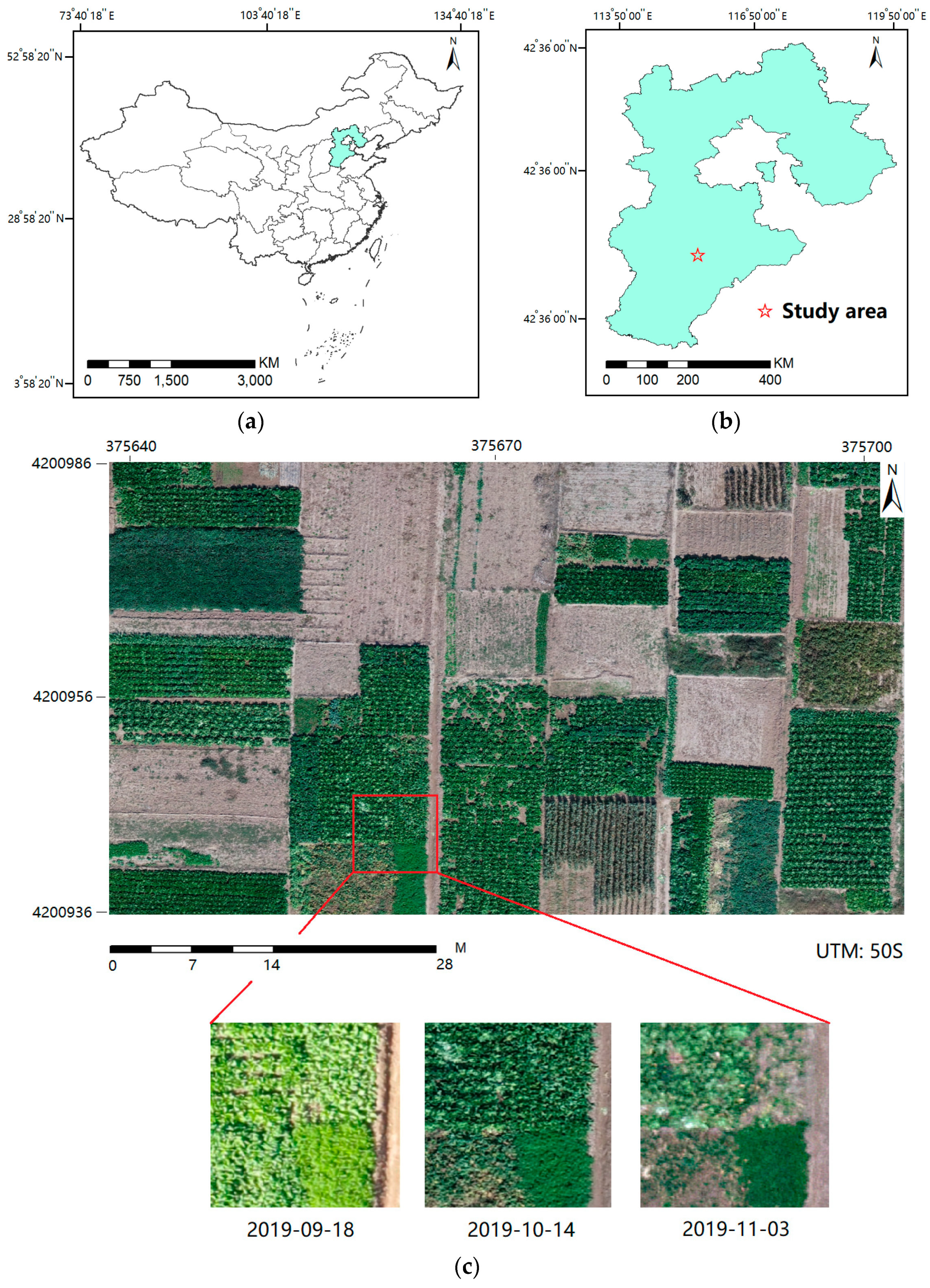
2.1. Study Area

Both the study area and multi-temporal UAV imagery used in this research are illustrated in Figure 1.
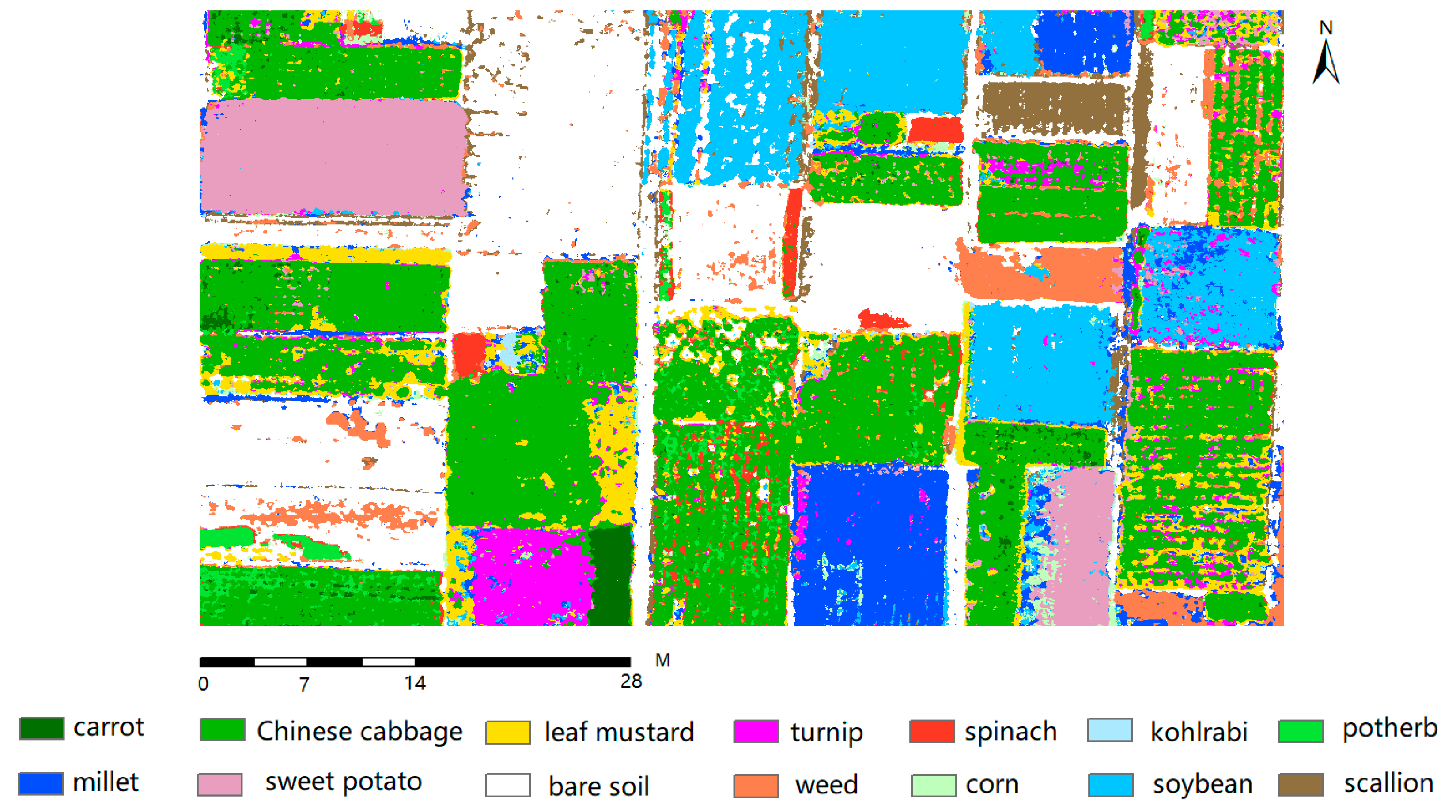
The study area includes a vegetable field which is located in Xijingmeng Village of Shenzhou City, Hebei province, China. There are various kinds of vegetables, such as Chinese cabbage, carrot, leaf mustard, etcetera. Meanwhile, the study area also locates in the North China Plain, which belongs to a continental monsoon climate, where summer is humid and hot, while winter is dry and cold. The annual temperature is about 13.4 °C and the annual precipitation is about 486 mm. Vegetables are usually planted in late August and harvested in early November.
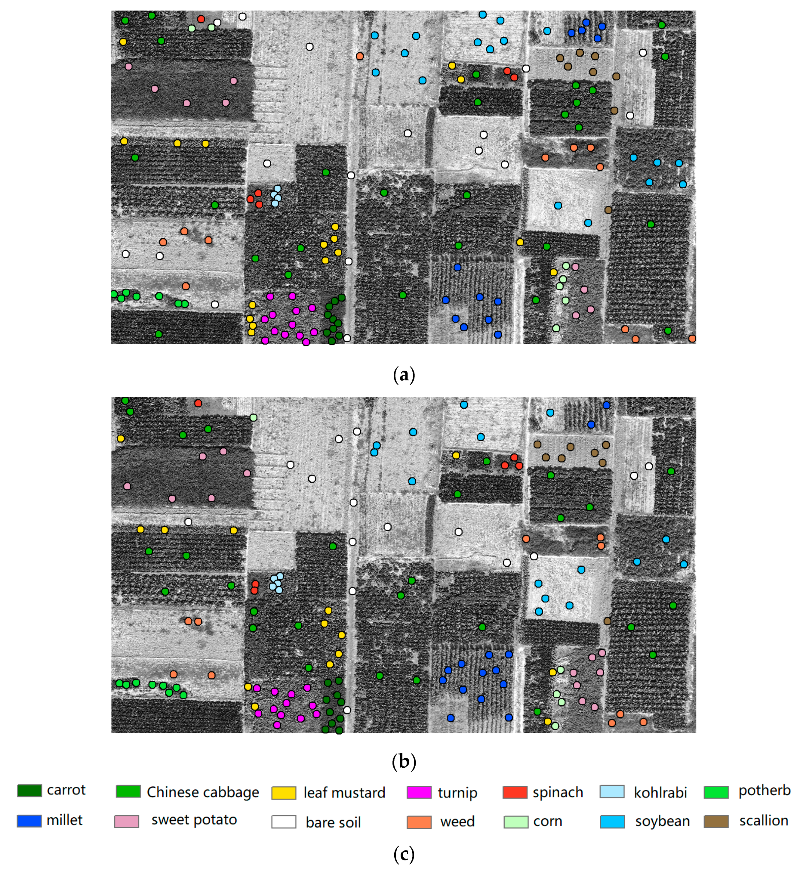
A field survey was conducted along with the UAV flight. Vegetable and crop types, locations measured by global positioning system (GPS) and photographs were recorded for every land parcel. According to the results of the field survey, there were a total of fourteen land cover categories, including eight vegetable types (i.e., carrot, Chinese cabbage, leaf mustard, turnip, spinach, kohlrabi, potherb and scallion), four crop types (i.e., millet, sweet potato, corn and soybean), weed and bare soil (Table 1).
Training and testing datasets were obtained from UAV imagery by visual inspection based on the sampling sites’ GPS coordinates and the corresponding land cover categories. Numbers of both training and testing datasets are shown in Table 1. Besides, Table 1 also shows the ground image taken during the field work to depict the detailed appearance of various vegetables and crops.
Meanwhile, Figure 2 illustrates the spatial distribution of both training and testing samples. It indicates that all the samples are randomly distributed and no overlap exists between training and testing regions. Besides, because we adopted patch-based per-pixel classification, all the training and testing samples are pixels from the region of interest (ROI). In this study, the number of training and testing samples are both 2250, respectively, which accounts for a small area (0.03%) of the total study region (7,105,350 pixels).

2.2. Dataset Used

We utilized a small-sized UAV, DJI-Inspire 2 [51], for the image data acquisition. The camera onboard is an off-the-shelf, light-weight digital camera with only three RGB bands. Therefore, the low spectral resolution would make it difficult to separate various vegetable categories if only considering single-date UAV data. To tackle this issue, we introduce multi-temporal UAV observations, which could obtain the phenological information during the growing season to increase the inter-class separability.
We conducted three flights in the autumn of 2019 (Table 2). During each flight, the flying height was set to be 80 m, achieving a very high spatial resolution of 2.5 cm/pixel. Besides, the width and height of the study area is 3535 and 2010 pixels (88.4 m and 50.3 m), respectively. Actually, the extent of the study area is at the limit of UAV data coverage. Although the study area may still seem small, it is limited by the operation range of the mini-UAV used. In future study, we would try high altitude long endurance (HALE) UAV to acquire images of a larger study region.
The raw images acquired during each flight were orthorectified firstly and then mosaicked to an entire image by Pix4D [52]. Specifically, several key parameters in Pix4D are set as follows. “Aerial Grid or Corridor” is chosen for matching image pairs, “Automatic” is selected for targeted number of key points, matching window size is 7 × 7 and 1 GSD is used for resolution. The rest of the parameters are set to default values. Afterwards, image registration was performed among the multi-temporal UAV data by ENVI (the Environment for Visualizing Images) [53].

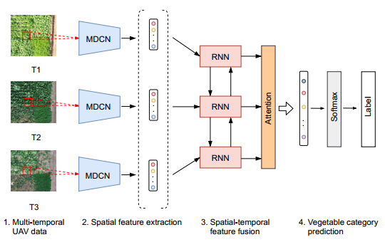
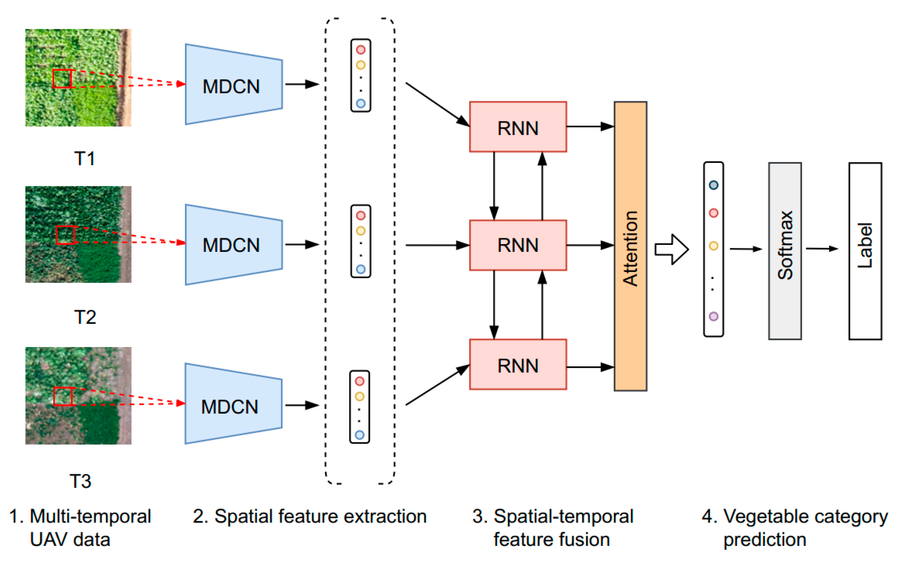
2.3. Overview of the ARCNN

Figure 3 illustrates the architecture of the proposed attention-based recurrent convolutional neural network (ARCNN) for vegetable mapping from multi-temporal UAV data. It mainly contains two parts, (1) a spatial feature extraction module based on a multi-scale deformable convolutional network (MDCN), and (2) a spatial-temporal feature fusion module based on a bi-directional RNN and attention mechanism. The former is to learn representative spatial features while the latter is to aggregate spatial and temporal features for the final vegetable classification.

2.4. Spatial Feature Extraction Based on MDCN

Accurate vegetable classification requires discriminative features. In this section, a multi-scale deformable convolutional network (MDCN) is proposed to learn and extract rich spatial features from UAV imagery, which is to account for the scale and shape variations of land parcels. Specifically, MDCN is an improved version of our previous study [44], and the network structure is depicted as Figure 4.
Same as our previous work, the input of MDCN is an image patch which is located at the center of the labeled pixel. The dimension of the patch is k × k × c [44], where k stands for the patch size while c refers to the channel number. Specifically, MDCN includes four regular convolutional layers and four deformable convolutional blocks. Table 3 shows the detailed configuration of the MDCN.
The deformable block contains multiple streams of deformable convolution [54], which could learn hierarchical and multi-scale features. The role of deformable convolution is to model the shape variations under complex agricultural landscapes. Considering that the standard convolution only samples the given feature map at fixed locations [54,55], it could not handle the geometric transformations. Compared with standard convolution, deformable convolution introduces additional offsets along with the standard sampling grid [54,55], which could account for various transformations for scale, aspect ratio and rotation, making it an ideal tool to extract robust features under complex landscapes. During the training process, both the kernel and offsets of a deformable convolution unit can be learned without additional supervision. In this situation, the output y at the location p0 could be calculated according to Equation (1):
y ( p 0 ) = w ( p i ) x ( p 0 + p i + Δ p i )
where w stands for the learned weights, pi means the i th location, x represents the input feature map and Δ p i refers to the offset to be learned [54]. In addition, as for the determination of the patch size k, we referred to our previous research [44] and the highest classification performance was reached when k equaled 11.

2.5. Spatial-Temporal Feature Fusion

After the extraction of spatial features from every mono-temporal UAV image, it is essential to establish the relationship between these sequential features to yield a complete feature representation for boosting the vegetable classification performance. In this section, we exploit an attention based bi-directional LSTM (Bi-LSTM-Attention) for the fusion of spatial and temporal features (Figure 5). The network structure of Bi-LSTM-Attention is illustrated as follows.
Specifically, LSTM is a variant of RNN, which contains one input layer, one or several hidden layers and one output layer [45]. It should be noted that LSTM is more specialized in capturing long-range dependencies between sequential signals than other RNN models. LSTM utilizes a vector (i.e., memory cell) to store the long-term memory and adopts a series of gates to control the information flow [45] (Figure 6). The hidden layer is updated as follows:
i t = σ ( W i x x t + W i h h t 1 + b i )
f t = σ ( W f x x t + W f h h t 1 + b f )
c t = f t c t 1 + i t tanh ( W c x x t + W c h h t 1 + b c )
o t = σ ( W o x x t + W o h h t 1 + b o )
h t = o t tanh ( c t )
where i refers to the input gate, f stands for the forget gate, o refers to the output gate, c is the memory cell and σ stands for the logistic sigmoid function [45].
LSTM has long been utilized in natural language processes (NLP) [56,57]. Recently, it has been introduced in the remote sensing field for change detection and land cover mapping. In this section, we exploit a bi-directional LSTM [57] to learn the relationship between multi-temporal spatial features extracted from the UAV image. As shown in Figure 5, two LSTMs are stacked together while the hidden state of first LSTM is fed into the second one, and the second LSTM follows a reverse order of the former to fully understand the dependencies of the sequential signals in a bi-directional way. In addition, to further improve the performance, we append an attention layer to the output of the second LSTM. Actually, attention mechanism is widely studied in the field of CV and NLP [58,59,60], which could automatically adjust the weight of input feature vectors according to their importance to the current task. Therefore, we also incorporate an attention layer to re-weight the sequential features to boost the classification performance.
Let H be a matrix containing a series of vectors [h1, h2, …, hT] that are produced by the bi-directional LSTM, where T denotes the length of the input features. The output of the attention layer is formed by a weighted sum of vectors described as follows:
M = tanh ( H )
α = s o f t m a x ( w T M )
R a t t = H α T
where α is the attention vector and while Ratt denotes the fused and attention-weighted spatial-temporal features. Additionally, the features outputted from the Bi-LSTM-Attention are re-weighted or re-calibrated adaptively, which could enhance the informative feature vectors and suppress the noisy and useless ones.
Finally, all the reweighted features were firstly sent to a fully-connected layer and then to a softmax classifier to predict the final vegetable category.

2.6. Details of Network Training

When training started, all the weights of the neural network were initialized through He normalization [61], and biases were all set to be zero. We adopt cross-entropy loss (Equation (10)) [62] as the loss function to train the proposed ARCNN:
C E = i y i p log ( y i )
where CE is short for cross-entropy loss, yp is the predicted result and y is one-hot representation of the ground-truth label. Adam [63] was utilized as the optimization method with a learning rate of 1 × 10⁻⁴. In the training procedure, the model with the lowest validation loss was saved.
We have conducted data augmentation to reduce the impact of limited labeled data in this study. Specifically, all training image patches were flipped and rotated by a random angle from 90°, 180° and 270°. Afterwards, we split 90% of the training datasets for the optimization of parameters. The remaining 10% of the training datasets were utilized as validation sets for performance evaluation during training. After the training process, a testing dataset was adopted to obtain the final classification accuracy.
Furthermore, we used TensorFlow [64] for the construction of our proposed model. The training process was performed on a computer running the Ubuntu 16.04 operation system. The central processing unit (CPU) involved as an Intel core i7-7800 @ 3.5 GHz while the graphics processing unit (GPU) was an NVIDIA GTX TitanX.

2.7. Accuracy Assessment

In this study, we utilized both qualitative and quantitative methods to verify the effectiveness of the proposed ARCNN for vegetable mapping. Specifically, as for the former, we used visual inspection to check for classification errors. While for the latter, a confusion matrix (CM) was obtained from the testing dataset. A series of metrics were calculated from the CM, including overall accuracy (OA), producer’s accuracy (PA), user’s accuracy (UA) and the Kappa coefficient.
As for the numbers of points chosen for each class, they were actually determined by the area ratio. For instance, the class of Chinese cabbage had the largest area ratio, therefore, the number of training/testing sample points was set to 400, which was the biggest among all the categories. Furthermore, other land cover types, such as spinach and kohlrabi, which only accounted for a small area on the entire study region, had a small number of sample points (only 50).
To further justify the effectiveness of the proposed method, we adopted both ablation analysis and comparison experiments with classic machine learning methods. Specifically, as for the ablation study, we justified the role of both attention-based RNN on vegetable mapping using the following setups. (1) Feature-stacking: concatenating or stacking the spatial features derived from each single-date data for classification; (2) Bi-LSTM: using a bi-directional LSTM for classification; (3) Bi-LSTM-Attention: using the attention-based bi-directional LSTM for classification and (4) standard convolution: using common, non-deformable convolution operations for classification. Besides, ablation study has also been done to justify the impact of deformable convolution when compared with the standard convolution operations.
Meanwhile, classic machine learning methods such as MLC, RF and SVM were also included for comparison experiments. In specific, MLC has long been studied in remote sensing image classification, where the predicted labels are generated based on the maximum likelihood when compared with the training samples. The basic assumption of MLC is that the training samples should follow the normal distribution, which is hard to satisfy in reality, resulting in a limited classification performance. RF belongs to an ensemble of decision trees and the predicted results are determined by the average output of each decision tree [65]. RF has no restrictions on training data distribution and has outperformed MLC in many remote sensing studies. As for SVM, it is based on the Vapnik–Chervonenkis (VC) dimension theory which aims at the minimization of structure risk, resulting in good performance, especially under the situation of limited data [66]. Parameters involved in SVM usually contain kernel type, penalty coefficient, etcetera.

3. Results

3.1. Results of Vegetable Mapping Based on Multi-Temporal Data

Figure 7 shows the vegetable mapping result generated from the proposed ARCNN. It manifests that the distribution of each vegetable category is close to field surveyed when compared with the ground truth (GT) map of Figure 8. The classification errors mainly lie between Chinese cabbage and leaf mustard, potherb, turnip and spinach.
In order to further visually justify the classification results, Figure 8 shows the ground truth map which is manually vectorized from the UAV data. Actually, when compared with the GT map, the classification map of Figure 7 shows a salt and pepper effect. On one side, the classification model in this research belongs to a per-pixel method, which does not consider the boundary information of each land parcel, resulting in a more scattered classification result. On the other hand, the GT map is an ideal description of the spatial extent of every land cover category, neglecting the variations within each land parcel. For instance, several weed regions are missing in the GT map due to small areas. Additionally the bare soil regions in some land parcels have also been neglected. However, in practice, based on the classification map of Figure 7, we could easily generate a land cover map which is more accurate and concise just like Figure 8, which would justify the value of the proposed method in vegetable mapping. To make the boundaries of each land parcel more accurate, in future study we will research semantic segmentation models such as fully convolutional neural networks [19] to improve the visual effect.
Meanwhile, to quantitatively assess the classification performance, the confusion matrix, Kappa coefficient, OA, PA and UA were derived from the testing dataset. Table 4 indicates that the proposed classification model shows a high performance with both a high OA (92.80%) and a high Kappa coefficient (0.9206).
Table 4 indicates that the omissions and commissions mainly exist among leaf mustard and Chinese cabbage, potherb and turnip. For instance, several leaf mustard pixels were misclassified as Chinese cabbage and vice versa. This was understandable, since both color and shape of these leafy green vegetables (Chinese cabbage, leaf mustard, potherb, etc.) are very similar, especially at the early growth stage. Meanwhile, the RGB image has the drawback of a low spectral resolution, making it hard to differentiate these vegetable categories when using only color and shape information. In addition, only a few mistakes occurred among the other categories, which verifies the effectiveness of the proposed vegetation mapping method.

3.2. Results of Vegetable Mapping Based on Mono-Temporal UAV Data

Figure 9 shows the vegetable map generated from both mono- and multi-temporal classification.
As mentioned above, one hypothesis of this study is that the inclusion of multi-temporal UAV data could provide additional phenological information, which would enhance the inter-class separability to cover the shortage of low spectral resolution caused by off-the-shelf digital cameras. Therefore, in this section, a contrast experiment was conducted to compare the performance between multi-temporal and mono-temporal classification. It should be noted that when using single-date UAV data for classification, the spatial-temporal feature fusion module (i.e., Bi-LSTM-Attention) would be non-functional during the training and testing procedure.
Figure 9 indicates that the incorporation of multi-temporal UAV images could significantly improve the classification performance when compared with mono-temporal data, which shows fewer obvious errors from visual inspection. This is in accordance with quantitative assessment (Table 5). It indicates that the overall classification accuracy improved by 19.76%–28.13%, with an average increase of 24.49%, after the inclusion of multi-temporal data.
Meanwhile, Figure 9 also shows that it is difficult to obtain a high-precision vegetable map if only utilizing single-date UAV RGB images. There would be a large amount of classification errors among different vegetable categories, especially between Chinese cabbage, leaf mustard and turnip. Specifically, during the early growth stage (T1), large amounts of Chinese cabbage and leaf mustard pixels are misclassified as turnip (Figure 9a). This is mainly because these leafy green vegetables share very similar appearances (e.g., color, shape and texture patterns), which leads to a low inter-class separability hence a poor classification accuracy (64.67%). In the middle growth stage (T2), the classification accuracy of Chinese cabbage has been greatly improved due to its shape change due to the growth process. However, it still remains difficult to separate leaf mustard from Chinese cabbage (Figure 9b). When it comes to the ripe stage (T3), the leaf mustard could finally be differentiated from Chinese cabbage (Figure 9c). This is mainly because the Chinese cabbage shows a round head in the ripe stage (Table 1), which is greatly different to leaf mustard.
Table 5 shows the class-level accuracy for each vegetable category and other land cover types. It indicates that there is a significant accuracy gap between mono- and multi-temporal classification when using UAV RGB imagery. This is understandable because if using single-date UAV data alone, the similarity of color and texture patterns between various vegetables would yield a low inter-class separability. This is even more so at the early growth stage (T1), when vegetable seedlings share very similar appearances, resulting in the lowest classification accuracy with an OA of 64.67%. However, with the inclusion of multi-temporal UAV images, the additional phenological information would increase the separability among various vegetables, which could boost the final classification performance.

3.3. Results of Ablation Analysis

To justify the effectiveness of the proposed ARCNN model, a series of ablation experiments are conducted and the results are shown as follows.

3.3.1. Results of Different Fusion Methods

In this section, we consider the following methods for the fusion of spatial-temporal features: (1) feature-stacking; (2) Bi-LSTM and (3) Bi-LSTM-Attention. The description of these methods is in Section 2.7. The experimental results are shown in Table 6.
Table 6 indicates that the Bi-LSTM-Attention module used in this study outperforms both feature-stacking and Bi-LSTM, which increases the OA by 3.24% and 1.87%, respectively. The role of Bi-LSTM-Attention will be discussed in Section 4.1.

3.3.2. Results of Standard Convolution

In this section, we replaced all the deformable convolution operations by standard convolution units in the proposed network to justify the role of deformable convolution in vegetable mapping. Table 7 shows the comparison results.
Table 7 implies that the inclusion of deformable convolution could improve the vegetable mapping accuracy. The detailed discussion will be presented in Section 4.2.

3.4. Results of Comparison with Other Methods

To further justify the effectiveness of the proposed classification model, we compared it with several machine learning classifiers and other deep learning models. As for the former, we conducted comparison experiments using MLC, RF and SVM based on the same training and testing datasets. We used grid search for the parameterization of both RF and SVM. It turns out that an RF with 300 decision trees and a max depth of 15, and a SVM with radial basis kernel, a gamma [66] of 0.001 and a penalty coefficient (C) [66] of 100 has the best performance, respectively.
Table 8 shows the comparison results between the proposed model and other classical machine learning methods. It indicates that the deep learning based model has an advantage over the classical methods. A detailed discussion of this will follow in Section 4.4.
In addition, we have conducted comparison experiments with several previous studies, mainly including Ndikumana et al. (stacked LSTMs) [46], Mou et al. (CNN-RNN) [47] and Ji et al. (3D-CNN) [43]. Because the dimension of input and output of these models are different from ours, we have made necessary changes accordingly when reproducing these DL models. The experimental results are shown as follows.
Table 9 indicates that the proposed ARCNN in the research has a better performance when compared with several previous deep learning models. The OA is boosted by an increase of 2.53% to 8.36% while the Kappa has risen by 2.78% to 9.23%. The detailed discussion will be presented in Section 4.4.

4. Discussion

4.1. Impact of Attention-Based RNN on Vegetable Mapping

In this section, we will discuss the impact of attention mechanisms in the RNN for vegetable mapping. Specifically, according to the ablation study results of Section 3.3.1, the comparisons were made between different methods for spatial-temporal feature fusion, including feature-stacking, Bi-LSTM and Bi-LSTM-Attention. Results show that the feature-stacking yields the lowest accuracy with an OA of 89.56% and a Kappa of 0.8849. The reason is that feature-stacking just concatenates all the multi-temporal features without considering the relationship and temporal dependencies across the sequential UAV data. Meanwhile, since Bi-LSTM could understand the dependencies of the sequential features in a bi-directional way, therefore, it shows a better performance than the simple feature-stacking method with an OA improvement of 1.37%. In this study, we added an attention layer on the top of Bi-LSTM to further improve its performance. The attention based Bi-LSTM could enhance the important features while suppressing the less informative ones, outperforming both feature-stacking and Bi-LSTM with an OA increase of 3.24% and 1.87%, respectively, which verifies its effectiveness in spatial-temporal feature fusion.

4.2. Impact of Deformable Convolution on Vegetable Mapping

Another hypothesis of this study is that the scale and shape variations could be accounted for using the deformable convolution. According to Table 7, it indicates that the inclusion of deformable convolution could boost the classification performance. The OA has been improved from 91.96% to 92.80% with a rise of about 1%, justifying the role of deformable convolution. The reason for the lower accuracy of standard convolution is that it has a fixed kernel shape, which lacks the capability to model the geometric transformations of complex landscapes. On the other hand, deformable convolution has a flexible receptive field, which could be adaptive to the variability of shape and scale of remotely sensed imagery [44]. Therefore, the deformable convolution shows a better performance, especially under the complex and fragmented agricultural landscape in this study.

4.3. Impact of Multi-Temporal UAV Data on Vegetable Mapping

In addition, we will further discuss the role of multi-temporal UAV data on vegetable mapping. In fact, one of the main objectives of this study is to explore whether the incorporation of multi-temporal UAV RGB images could improve the vegetable classification accuracy. The initial motivation lies in the fact that RGB images acquired by UAV have a low spectral resolution, which would make it hard for the fine-grained classification of various vegetable categories. Therefore, in this study we have selected images from three important periods, i.e., the sowing period, the growing period and the harvesting period, to capture the phenological characteristics of different vegetables. Although the number of three dates may seem limited, all of them fall into the distinct periods of the vegetable and crop growth stage, which could still provide additional and useful time-series features for classification.
Meanwhile, in previous studies, images from only three dates have been studied for remote sensing image classification and they outperform the single-date dataset. For instance, Palchowdhuri et al. used three images from both multi-temporal Sentinel-2 and WordView-3 imagery for crop classification in Coalville in the United Kingdom and achieved an accuracy of 91% [67]. Similar findings were also reported in Yang et al., where three images from summer, autumn and winter were integrated for coastal land cover mapping [68]. In our previous study [15], we also utilized only three images during the whole crop growing season for the cropland classification in the Yellow River Delta of China, which yielded an average accuracy of 89%, justifying the role of three dates for classification. In future research, images from a longer temporal range could be included to further improve the classification performance.

4.4. Comparison with Other Methods

In this section, we focused on the detailed discussion between the proposed ARCNN and other classical machine learning methods and several previous deep learning methods. Specifically, Table 8 indicates that our proposed method outperforms machine learning methods such as MLC, RF and SVM with an OA increase of 27.29%, 21.58% and 8.64%, respectively. The results are in accordance with [46] and our previous studies [39,44]. The reason could be that classical machine learning methods lack the ability to capture the high-level representative features when compared to deep learning models, leading to a performance gap in vegetable mapping.
In addition, there is a need to compare the proposed ARCNN with other methods for multi-temporal UAV image classification. Recent researches such as van Iersel et al. [14] and Michez et al. [12], they both utilized object-oriented image analysis (OBIA) and random forest for plant classification from multi-date UAV data. Manually designed features such as band ratio and vegetation indices were used for classification. Compared with their studies, we replace the manually designed features with high-level and discriminative features that are automatically learned from deep neural networks, (i.e., CNN and RNN), which could enhance the feature’s representativeness. To the best of our knowledge, this study is the first case to introduce deep learning methods in multi-temporal UAV image classification. Therefore, the proposed method in this research might provide useful reference for future studies.
Meanwhile, it is also necessary to compare the proposed ARCNN with other deep learning models for remote sensing image classification. Early studies mainly utilized LSTM for multi-temporal classification. One representative research is Ndikumana et al., where five LSTMs were stacked for the classification using multi-temporal SAR Sentinel-1 data [46]. The input data in Ndikumana’s study are a single pixel with a time curve, which neglects the rich, contextual relationship hidden in the spatial features, showing a relatively lower accuracy (84.44%). Different from Ndikumana et al. [46], we have added a CNN in front of LSTM to enrich the representative spatial feature extraction.
Mou et al. also cascaded a CNN and RNN for change detection from two optical remote sensing images [47]. Compared with Mou et al. [47], our model makes two significant improvements. Firstly, from the perspective of CNN, we incorporate the multi-scale deformable convolutions, which could aggregate multi-level contextual features. Secondly, we used the attention mechanism with a bi-directional LSTM to further enhance the modeling of sequential signals in multi-temporal remote sensing data. All the above modifications have improved the classification from 90.18% by Mou et al. to 92.80%.
Besides, Ji et al. adopted a 3D-CNN to extract spatial-temporal features for crop type mapping from multi-temporal satellite imagery [43]. Compared with Ji et al. [43], our method has also gained a more accurate result. The reason lies in that 3D CNN cannot explicitly establish the relationship between the sequential signals, which has flaws in the generation of spatial-temporal feature fusion and integration. Furthermore, our Bi-LSTM-Attention module is more straightforward in mining the relationship across multi-temporal data than a 3D-CNN.

5. Conclusions

This study proposed an attention-based recurrent convolutional neural network (ARCNN) for accurate vegetable mapping based on multi-temporal unmanned aerial vehicle (UAV) red-green-blue (RGB) data. The proposed ARCNN first leverages a multi-scale deformable CNN to learn and extract the rich spatial features from each mono-temporal UAV image, which aims to account for the shape and scale variations under complex and fragmented agricultural landscapes. Afterwards, an attention-based bi-directional long-short term memory (LSTM) is introduced to model the relationship between the sequential features, from which spatial and temporal features are fused and aggregated. Finally, the fused features are fed to a fully connected layer and a softmax classifier to determine the vegetable category.
Experimental results showed that the proposed ARCNN yields a high classification performance with an overall accuracy (OA) of 92.08% and a Kappa coefficient of 0.9206. When compared with mono-temporal classification, the incorporation of multi-temporal UAV data could boost the OA significantly by an average increase of 24.49%, which verifies the hypothesis that multi-temporal UAV observations could enhance the inter-class separability and thus reduce the drawback of low spectral resolution of off-the-shelf digital cameras. The Bi-LSTM-Attention module outperforms other fusion methods such as feature-staking and bi-directional LSTM with an OA increase of 3.24% and 1.87%, respectively, justifying its effectiveness in modeling the dependency across the sequential features. Meanwhile, the introduction of deformable convolution could also improve the OA by about 1% when compared with standard convolution. In addition, the proposed ARCNN also shows a higher performance than other classical machine learning classifiers such as maximum likelihood classifier, random forest and support vector machine, and several previous deep learning methods for remote sensing classification.
This study demonstrates that the proposed ARCNN could yield an accurate vegetable mapping result from multi-temporal UAV RGB data. The drawback of low spectral resolution of RGB images could be compensated by introducing additional phenological information and robust deep learning models. Although images from only three dates were included, a good classification result could still be achieved providing all three dates fall into the distinct growing periods of vegetables. Finally, the proposed model could be viewed as a general framework for multi-temporal remote sensing image classification. As for future work, more study cases should be considered to justify the effectiveness of the proposed method. Additionally, semantic segmentation models should be incorporated to get a more accurate vegetable map.

Author Contributions

Methodology, Q.F.; validation, Q.F. and J.Y.; data curation, Y.L. and C.O.; writing—original draft preparation, Q.F.; writing—review and editing, J.Y., D.Z., B.N., J.L. and B.L. All authors have read and agreed to the published version of the manuscript.

Funding

This research was funded by the China Postdoctoral Science Foundation, grant number 2018M641529, 2019T120155 and the National Key Research and Development Program of China, grant number 2018YFE0122700.

Acknowledgments

Special thanks to the anonymous reviewers and editors for their very useful comments and suggestions to help improve the quality of this paper. The authors give thanks to Zhe Liu from the China Agricultural University for assisting in the field work. We would also like to thank Beijing IRIS Remote Sensing Technology Limited, Inc. for their help in preprocessing UAV raw data.

Conflicts of Interest

The authors declare no conflict of interest.

References

  1. Torres-Sánchez, T.; Peña, J.M.; de Castro, A.I.; López-Granados, F. Multi-temporal mapping of the vegetation fraction in early-season wheat fields using images from UAV. Comput. Electron. Agric. 2014, 103, 104–113. [Google Scholar] [CrossRef]
  2. Wikantika, K.; Uchida, S.; Yamamoto, S. Mapping vegetable area with spectral mixture analysis of the Landsat-ETM. In Proceedings of the IEEE International Geoscience and Remote Sensing Symposium, Toronto, ON, Canada, 24–28 June 2002; pp. 1965–1967. [Google Scholar]
  3. Belgiu, M.; Csillik, O. Sentinel-2 cropland mapping using pixel-based and object-based time-weighted dynamic time warping analysis. Remote Sens. Environ. 2018, 204, 509–523. [Google Scholar] [CrossRef]
  4. Rupasinghe, P.A.; Milas, A.S.; Arend, K.; Simonson, M.A.; Mayer, C.; Mackey, S. Classification of shoreline vegetation in the Western Basin of Lake Erie using airborne hyperspectral imager HSI2, Pleiades and UAV data. Int. J. Remote Sens. 2019, 40, 3008–3028. [Google Scholar] [CrossRef]
  5. Wan, S.; Chang, S.H. Crop classification with WorldView-2 imagery using Support Vector Machine comparing texture analysis approaches and grey relational analysis in Jianan Plain, Taiwan. Int. J. Remote Sens. 2019, 40, 8076–8092. [Google Scholar] [CrossRef]
  6. Asgarian, A.; Soffianian, A.; Pourmanafi, S. Crop type mapping in a highly fragmented and heterogeneous agricultural landscape: A case of central Iran using multi-temporal Landsat 8 imagery. Comput. Electron. Agric. 2016, 127, 531–540. [Google Scholar] [CrossRef]
  7. Feng, Q.; Liu, J.; Gong, J. UAV remote sensing for urban vegetation mapping using random forest and texture analysis. Remote Sens. 2015, 7, 1074–1094. [Google Scholar] [CrossRef] [Green Version]
  8. Feng, Q.; Liu, J.; Gong, J. Urban flood mapping based on unmanned aerial vehicle remote sensing and random forest classifier—A case of Yuyao, China. Water 2015, 7, 1437–1455. [Google Scholar] [CrossRef]
  9. Dai, Y.; Gong, J.; Li, Y.; Feng, Q. Building segmentation and outline extraction from UAV image-derived point clouds by a line growing algorithm. Int. J. Digit. Earth 2017, 10, 1077–1097. [Google Scholar] [CrossRef]
  10. Böhler, J.E.; Schaepman, M.E.; Kneubühler, M. Optimal timing assessment for crop separation using multispectral unmanned aerial vehicle (UAV) data and textural features. Remote Sens. 2019, 11, 1780. [Google Scholar] [CrossRef] [Green Version]
  11. Pádua, L.; Marques, P.; Hruška, J.; Adão, T.; Peres, E.; Morais, R.; Sousa, J.J. Multi-temporal vineyard monitoring through UAV-based RGB imagery. Remote Sens. 2018, 10, 1907. [Google Scholar] [CrossRef] [Green Version]
  12. Michez, A.; Piégay, H.; Lisein, J.; Claessens, H.; Lejeune, P. Classification of riparian forest species and health condition using multi-temporal and hyperspatial imagery from unmanned aerial system. Environ. Monit. Assess. 2016, 188, 146. [Google Scholar] [CrossRef] [PubMed] [Green Version]
  13. Moeckel, T.; Dayananda, S.; Nidamanuri, R.R.; Nautiyal, S.; Hanumaiah, N.; Buerkert, A.; Wachendorf, M. Estimation of vegetable crop parameter by multi-temporal UAV-borne images. Remote Sens. 2018, 10, 805. [Google Scholar] [CrossRef] [Green Version]
  14. Van Iersel, W.; Straatsma, M.; Middelkoop, H.; Addink, E. Multitemporal Classification of river floodplain vegetation using time series of UAV images. Remote Sens. 2018, 10, 1144. [Google Scholar] [CrossRef] [Green Version]
  15. Feng, Q.; Gong, J.; Liu, J.; Li, Y. Monitoring cropland dynamics of the yellow river delta based on multi-temporal Landsat imagery over 1986 to 2015. Sustainability 2015, 7, 14834–14858. [Google Scholar] [CrossRef] [Green Version]
  16. Chen, L.; Yang, W.; Xu, K.; Xu, T. Evaluation of local features for scene classification using VHR satellite images. In Proceedings of the 2011 Joint Urban Remote Sensing Event, Munich, Germany, 11–13 April 2011; pp. 385–388. [Google Scholar]
  17. Zhu, Q.; Zhong, Y.; Zhao, B.; Xia, G.; Zhang, L. Bag-of-visual-words scene classifier with local and global features for high spatial resolution remote sensing imagery. IEEE Geosci. Remote Sens. Lett. 2016, 13, 747–751. [Google Scholar] [CrossRef]
  18. LeCun, Y.; Bengio, Y.; Hinton, G. Deep learning. Nature 2015, 521, 436–444. [Google Scholar] [CrossRef]
  19. Shelhamer, E.; Long, J.; Darrell, T. Fully convolutional networks for semantic segmentation. IEEE Trans. Pattern Anal. Mach. Intell. 2017, 39, 640–651. [Google Scholar] [CrossRef]
  20. LaLonde, R.; Bagci, U. Capsules for Object Segmentation. arXiv 2018, arXiv:1804.04241. Available online: https://arxiv.org/abs/1804.04241.pdf (accessed on 17 April 2020).
  21. Lin, T.Y.; Goyal, P.; Girshick, R.; He, K.; Dollar, P. Focal loss for dense object detection. In Proceedings of the IEEE International Conference on Computer Vision (ICCV), Venice, Italy, 22–29 October 2017; pp. 2999–3007. [Google Scholar]
  22. Krizhevsky, A.; Sutskever, I.; Hinton, G.E. Imagenet classification with deep convolutional neural networks. Proc. Adv. Neural Inf. Process. Syst. 2012, 1097–1105. [Google Scholar] [CrossRef]
  23. He, K.; Zhang, X.; Ren, S.; Sun, J. Deep residual learning for image recognition. In Proceedings of the IEEE Conference on Computer Vision and Pattern Recognition, Las Vegas, NV, USA, 27–30 June 2016; pp. 770–778. [Google Scholar]
  24. Hu, J.; Shen, L.; Sun, G. Squeeze-and-Excitation Networks. arXiv 2017, arXiv:1709.01507. Available online: https://arxiv.org/pdf/1709.01507.pdf (accessed on 17 April 2020).
  25. Zhu, X.X.; Tuia, D.; Mou, L.; Xia, G.; Zhang, L.; Xu, F.; Fraundorfer, F. Deep learning in remote sensing: A comprehensive review and list of resources. IEEE Geosci. Remote Sens. Mag. 2017, 5, 8–36. [Google Scholar] [CrossRef] [Green Version]
  26. Zhang, L.; Zhang, L.; Du, B. Deep learning for remote sensing data: A technical tutorial on the state of the art. IEEE Geosci. Remote Sens. Mag. 2016, 4, 22–40. [Google Scholar] [CrossRef]
  27. Kellenberger, B.; Marcos, D.; Tuia, D. Detecting mammals in UAV images: Best practices to address a substantially imbalanced dataset with deep learning. Remote Sens. Environ. 2018, 216, 139–153. [Google Scholar] [CrossRef] [Green Version]
  28. Carrio, A.; Sampedro, C.; Rodriguez-Ramos, A.; Campoy, P. A review of deep learning methods and applications for unmanned aerial vehicles. J. Sens. 2017, 3296874. [Google Scholar] [CrossRef]
  29. Kamilaris, A.; Prenafeta-Boldú, F.X. Deep learning in agriculture: A survey. Comput. Electron. Agric. 2018, 147, 70–90. [Google Scholar] [CrossRef] [Green Version]
  30. Chen, Y.; Fan, R.; Bilal, M.; Yang, X.; Wang, J.; Li, W. Multilevel cloud detection for high-resolution remote sensing imagery using multiple convolutional neural networks. ISPRS Int. J. Geo. Inf. 2018, 7, 181. [Google Scholar] [CrossRef] [Green Version]
  31. Alshehhi, R.; Marpu, P.R.; Woon, W.L.; Mura, M.D. Simultaneous extraction of roads and buildings in remote sensing imagery with convolutional neural networks. ISPRS J. Photogramm. Remote Sens. 2017, 130, 139–149. [Google Scholar] [CrossRef]
  32. Xu, Y.; Wu, L.; Xie, Z.; Chen, Z. Building Extraction in Very High Resolution Remote Sensing Imagery Using Deep Learning and Guided Filters. Remote Sens. 2018, 10, 144. [Google Scholar] [CrossRef] [Green Version]
  33. Li, X.; Yao, X.; Fang, Y. Building-A-Nets: Robust Building Extraction From High-Resolution Remote Sensing Images With Adversarial Networks. IEEE J. Sel. Top. Appl. Earth Obs. Remote Sens. 2018, 11, 3680–3687. [Google Scholar] [CrossRef]
  34. Deng, Z.; Sun, H.; Zhou, S.; Zhao, J.; Zou, H. Toward Fast and Accurate Vehicle Detection in Aerial Images Using Coupled Region-Based Convolutional Neural Networks. IEEE J. Sel. Top. Appl. Earth Obs. Remote Sens. 2017, 10, 3652–3664. [Google Scholar] [CrossRef]
  35. Ammour, N.; Alhichri, H.; Bazi, Y.; Benjdira, B.; Alajlan, N.; Zuair, M. Deep Learning Approach for Car Detection in UAV Imagery. Remote Sens. 2017, 9, 312. [Google Scholar] [CrossRef] [Green Version]
  36. Han, W.; Feng, R.; Wang, L.; Cheng, Y. A semi-supervised generative framework with deep learning features for high-resolution remote sensing image scene classification. ISPRS J. Photogramm. Remote Sens. 2018, 145, 23–43. [Google Scholar] [CrossRef]
  37. Wang, Q.; Liu, S.; Chanussot, J.; Li, X. Scene classification with recurrent attention of VHR remote sensing images. IEEE Trans. Geosci. Remote Sens. 2019, 57, 1155–1167. [Google Scholar] [CrossRef]
  38. Rußwurm, M.; Körner, M. Multi-temporal land cover classification with sequential recurrent encoders. ISPRS Int. J. Geo. Inf. 2018, 7, 129. [Google Scholar] [CrossRef] [Green Version]
  39. Feng, Q.; Zhu, D.; Yang, J.; Li, B. Multisource hyperspectral and LiDAR data fusion for urban land-use mapping based on a modified two-branch convolutional neural network. ISPRS Int. J. Geo. Inf. 2019, 8, 28. [Google Scholar] [CrossRef] [Green Version]
  40. Huang, B.; Zhao, B.; Song, Y. Urban land-use mapping using a deep convolutional neural network with high spatial resolution multispectral remote sensing imagery. Remote Sens. Environ. 2018, 214, 73–86. [Google Scholar] [CrossRef]
  41. Kussul, N.; Lavreniuk, M.; Skakun, S.; Shelestov, A. Deep learning classification of land cover and crop types using remote sensing data. IEEE Geosci. Remote Sens. Lett. 2017, 14, 778–782. [Google Scholar] [CrossRef]
  42. Rezaee, M.; Mahdianpari, M.; Zhang, Y.; Salehi, B. Deep convolutional neural network for complex wetland classification using optical remote sensing imagery. IEEE J. Sel. Top. Appl. Earth Obs. Remote Sens. 2018, 11, 3030–3039. [Google Scholar] [CrossRef]
  43. Ji, S.; Zhang, C.; Xu, A.; Shi, Y.; Duan, Y. 3D convolutional neural networks for crop classification with multi-temporal remote sensing images. Remote Sens. 2018, 10, 75. [Google Scholar] [CrossRef] [Green Version]
  44. Feng, Q.; Yang, J.; Zhu, D.; Liu, J.; Guo, H.; Bayartungalag, B.; Li, B. Integrating multitemporal sentinel-1/2 data for coastal land cover classification using a multibranch convolutional neural network: A case of the Yellow River Delta. Remote Sens. 2019, 11, 1006. [Google Scholar] [CrossRef] [Green Version]
  45. Hochreiter, S.; Schmidhuber, J. Long short-term memory. Neural Comput. 1997, 9, 1735–1780. [Google Scholar] [CrossRef] [PubMed]
  46. Ndikumana, E.; Ndikumana, E.; Ho Tong Minh, D.; Baghdadi, N.; Courault, D.; Hossard, L. Deep recurrent neural network for agricultural classification using multitemporal SAR Sentinel-1 for Camargue, France. Remote Sens. 2018, 10, 1217. [Google Scholar] [CrossRef] [Green Version]
  47. Mou, L.; Bruzzone, L.; Zhu, X.X. Learning spectral-spatial-temporal features via a recurrent convolutional neural network for change detection in multispectral imagery. IEEE Trans. Geosci. Remote Sens. 2019, 57, 924–935. [Google Scholar] [CrossRef] [Green Version]
  48. Song, A.; Choi, J.; Han, Y.; Kim, Y. Change detection in hyperspectral images using recurrent 3D fully convolutional networks. Remote Sens. 2018, 10, 1827. [Google Scholar] [CrossRef] [Green Version]
  49. Liu, Q.; Zhou, F.; Hang, R.; Yuan, X. Bidirectional-convolutional LSTM based spectral-spatial feature learning for hyperspectral image classification. Remote Sens. 2017, 9, 1330. [Google Scholar]
  50. Mou, L.; Ghamisi, P.; Zhu, X.X. Deep recurrent neural networks for hyperspectral image classification. IEEE Trans. Geosci. Remote Sens. 2017, 55, 3639–3655. [Google Scholar] [CrossRef] [Green Version]
  51. DJI-Inspire 2. Available online: https://www.dji.com/cn/inspire-2/ (accessed on 17 March 2020).
  52. Pix4D. Available online: http://pix4d.com/ (accessed on 17 March 2020).
  53. ENVI. Available online: http://www.enviidl.com/ (accessed on 17 March 2020).
  54. Dai, J.; Qi, H.; Xiong, Y.; Li, Y.; Zhang, G.; Hu, H.; Wei, Y. Deformable convolutional networks. arXiv 2017, arXiv:1703.06211. Available online: https://arxiv.org/abs/1703.06211 (accessed on 17 March 2020).
  55. Jin, Q.; Meng, Z.; Pham, T.D.; Chen, Q.; Wei, L.; Su, R. DUNet: A Deformable Network for Retinal Vessel Segmentation. arXiv 2018, arXiv:1811.01206. Available online: https://arxiv.org/pdf/1811.01206.pdf (accessed on 17 April 2020). [CrossRef] [Green Version]
  56. Pan, D.; Yuan, J.; Li, L.; Sheng, D. Deep neural network-based classification model for Sentiment Analysis. arXiv 2019, arXiv:1907.02046. Available online: https://arxiv.org/abs/1907.02046 (accessed on 17 April 2019).
  57. Melamud, O.; Goldberger, J.; Dagan, I. Context2vec: Learning generic context embedding with bidirectional LSTM. In Proceedings of the 20th SIGNLL Conference on Computational Natural Language Learning (CoNLL), Berlin, Germany, 11–12 August 2016; pp. 51–61. [Google Scholar]
  58. Cui, W.; Wang, F.; He, X.; Zhang, D.; Xu, X.; Yao, M.; Wang, Z.; Huang, J. Multi-scale semantic segmentation and spatial relationship recognition of remote sensing images based on an attention model. Remote Sens. 2019, 11, 1044. [Google Scholar] [CrossRef] [Green Version]
  59. Xu, R.; Tao, Y.; Lu, Z.; Zhong, Y. Attention-mechanism-containing neural networks for high-resolution remote sensing image classification. Remote Sens. 2018, 10, 1602. [Google Scholar] [CrossRef] [Green Version]
  60. Zhao, B.; Wu, X.; Feng, J.; Peng, Q.; Yan, S. Diversified visual attention networks for fine-grained object classification. IEEE Trans. Multimedia 2017, 19, 1245–1256. [Google Scholar] [CrossRef] [Green Version]
  61. He, K.; Zhang, X.; Ren, S.; Sun, J. Delving deep into rectifiers: Surpassing human-level performance on ImageNet classification. arXiv 2015, arXiv:1502.01852. Available online: https://arxiv.org/pdf/1502.01852.pdf (accessed on 17 March 2020).
  62. Cox, D. The Regression Analysis of Binary Sequences. J. Royal Stat. Soc. Ser. B 1958, 20, 215–242. [Google Scholar] [CrossRef]
  63. Kingma, D.P.; Ba, J. Adam: A Method for Stochastic Optimization. arXiv 2014, arXiv:1412.6980. Available online: https://arxiv.org/abs/1412.6980 (accessed on 17 March 2020).
  64. TensorFlow. Available online: https://tensorflow.google.cn/ (accessed on 17 March 2020).
  65. Breiman, L. Random forests. Mach. Learn. 2001, 45, 5–32. [Google Scholar] [CrossRef] [Green Version]
  66. Chapelle, O.; Vapnik, V.; Bousquet, O.; Mukherjee, S. Choosing multiple parameters for support vector machines. Mach. Learn. 2002, 46, 131–159. [Google Scholar] [CrossRef]
  67. Palchowdhuri, Y.; Valcarce-Diñeiro, R.; King, P.; Sanabria-Soto, M. Classification of multi-temporal spectral indices for crop type mapping: A case study in Coalville, UK. J. Agric. Sci. 2018, 156, 24–36. [Google Scholar] [CrossRef]
  68. Yang, X.; Chen, L.; Li, Y.; Xi, W.; Chen, L. Rule-based land use/land cover classification in coastal areas using seasonal remote sensing imagery: A case study from Lianyungang City, China. Environ. Monit. Assess. 2015, 187, 449. [Google Scholar] [CrossRef]
Figure 1. Study area. (a) China; (b) Hebei Province; and (c) Xijingmeng Village and multi-temporal UAV images.
Remotesensing 12 01668 g001
Figure 2. Spatial distribution of (a) training samples; (b) testing samples; (c) legend.
Remotesensing 12 01668 g002
Figure 3. The overview of the proposed attention-based recurrent convolutional neural network (ARCNN) for vegetable mapping based on multi-temporal UAV data.
Remotesensing 12 01668 g003
Figure 4. (a) Network structure of the proposed multi-scale deformable convolutional network (MDCN); (b) deformable convolutional block; (c) standard convolution; and (d) deformable convolution.
Remotesensing 12 01668 g004
Figure 5. Architecture of the attention-based bi-directional LSTM.
Remotesensing 12 01668 g005
Figure 6. Structure of the LSTM.
Remotesensing 12 01668 g006
Figure 7. Vegetable map generated from the proposed ARCNN and multi-temporal UAV RGB datasets.
Remotesensing 12 01668 g007
Figure 8. Ground truth map vectorized from the UAV data.
Remotesensing 12 01668 g008
Figure 9. Vegetable map generated from (a) T1/2019-09; (b) T2/2019-10; (c) T3/2019-11 and (d) multi-temporal datasets using the proposed method. (e) Legend.
Remotesensing 12 01668 g009
Table 1. Classification scheme of this study.
No.Class NameTraining/TestingGround ImageNo.Class NameTraining/TestingGround Image
1Carrot200/200 Remotesensing 12 01668 i0018Millet200/200 Remotesensing 12 01668 i002
2Chinese cabbage400/400 Remotesensing 12 01668 i0039Weed100/100 Remotesensing 12 01668 i004
3Leaf mustard200/200 Remotesensing 12 01668 i00510Bare soil200/200 Remotesensing 12 01668 i006
4Turnip200/200 Remotesensing 12 01668 i00711Sweet potato200/200 Remotesensing 12 01668 i008
5Spinach50/50 Remotesensing 12 01668 i00912Corn50/50 Remotesensing 12 01668 i010
6Kohlrabi50/50 Remotesensing 12 01668 i01113Soybean200/200 Remotesensing 12 01668 i012
7Potherb100/100 Remotesensing 12 01668 i01314Scallion100/100 Remotesensing 12 01668 i014
Table 2. Multi-temporal UAV images utilized in this study.
SeasonDateData Source
T1Autumn18 September 2019UAV RGB data
T2Autumn14 October 2019UAV RGB data
T3Autumn3 November 2019UAV RGB data
Table 3. Detailed configuration of the MDCN.
Layer NameInput SizeOutput SizeKernel SizeFilter NumberStride
Input11 × 11 × 3--------
Conv111 × 11 × 311 × 11 × 643 × 3641
Conv211 × 11 × 6411 × 11 × 1283 × 31281
Conv311 × 11 × 1286 × 6 × 1283 × 31282
Deform Block 16 × 6 × 1286 × 6 × 128------
Deform Block 26 × 6 × 1286 × 6 × 128------
Conv46 × 6 × 1283 × 3 × 1283 × 32562
Deform Block 33 × 3 × 2563 × 3 × 256------
Deform Block 43 × 3 × 2563 × 3 × 256------
Table 4. Confusion matrix.
ClassGround Truth
1234567891011121314UA
1200900000000000095.7
20353213000000000093.6
303614912000000000075.6
40071820001600004087.1
5000050000000000100
6000005000000000100
70016000100000000086.2
8002000018400080094.8
90000000010000000100
10000000000200020994.8
110000000000200000200
1200010000000330097.1
13025200000007196092.5
14000000000000091100
PA10088.374.591.010010010092.010010010066.098.091.0
OA92.80Kappa0.9206
1: carrot; 2: Chinese cabbage; 3: leaf mustard; 4: turnip; 5: spinach; 6: kohlrabi; 7: potherb; 8: millet; 9: weed; 10: bare soil; 11: sweet potato; 12: corn; 13: soybean; 14: scallion; PA: producer’s accuracy; UA: user’s accuracy and OA: overall accuracy.
Table 5. Class-level accuracy for mono- and multi-temporal classification.
No.Class NameT1 (%)T2 (%)T3 (%)Proposed (%)
1Carrot89.0093.0084.00100
2Chinese cabbage46.5068.5077.2588.25
3Leaf mustard29.0039.0050.0074.50
4Turnip59.0043.5075.0091.00
5Spinach--38.0018.00100
6Kohlrabi22.0034.00--100
7Potherb--25.0057.00100
8Millet73.5076.50--92.00
9Weed75.0095.0085.00100
10Bare soil92.5094.5079.00100
11Sweet potato55.5084.00--100
12Corn78.0076.00--66.00
13Soybean75.0049.00--98.00
14Scallion95.00----91.00
OA (%)64.6767.2273.0492.80
Kappa0.60670.63140.67440.9206
Table 6. Comparison between different spatial-temporal feature fusion methods.
MethodOA (%)Kappa
Feature-stacking89.560.8849
Bi-LSTM90.930.8999
Bi-LSTM-Attention92.800.9206
Table 7. Comparison of standard and deformable convolution.
MethodOA (%)Kappa
Standard convolution91.960.9111
Deformable convolution92.800.9206
Table 8. Comparison with classical machine learning classifiers.
MethodOA (%)Kappa
MLC46.040.4095
RF63.960.6023
SVM84.760.8317
Proposed92.800.9206
Table 9. Comparison with other deep learning methods.
MethodOA (%)Kappa
Ndikumana et al.84.440.8283
Mou et al.90.270.8928
Ji et al.90.180.8915
Proposed92.800.9206

