Automatic Processing of Aerial LiDAR Data to Detect Vegetation Continuity in the Surroundings of Roads

 , , and
Abstract
:
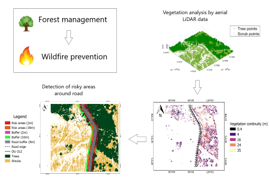
1. Introduction
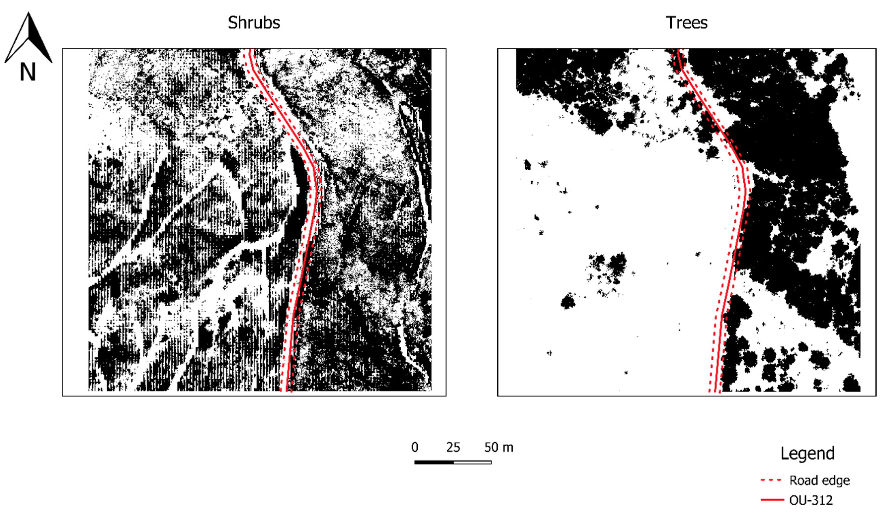
- Determination of criteria to classify vegetation points into two groups—shrubs and trees;
- Development of a series of algorithms to automatically calculate the Canopy Cover Fraction (CCF) and the Canopy Relief Ratio (CRR);
- Determination of the accuracy of the used methodology by comparison with the ground truth data;
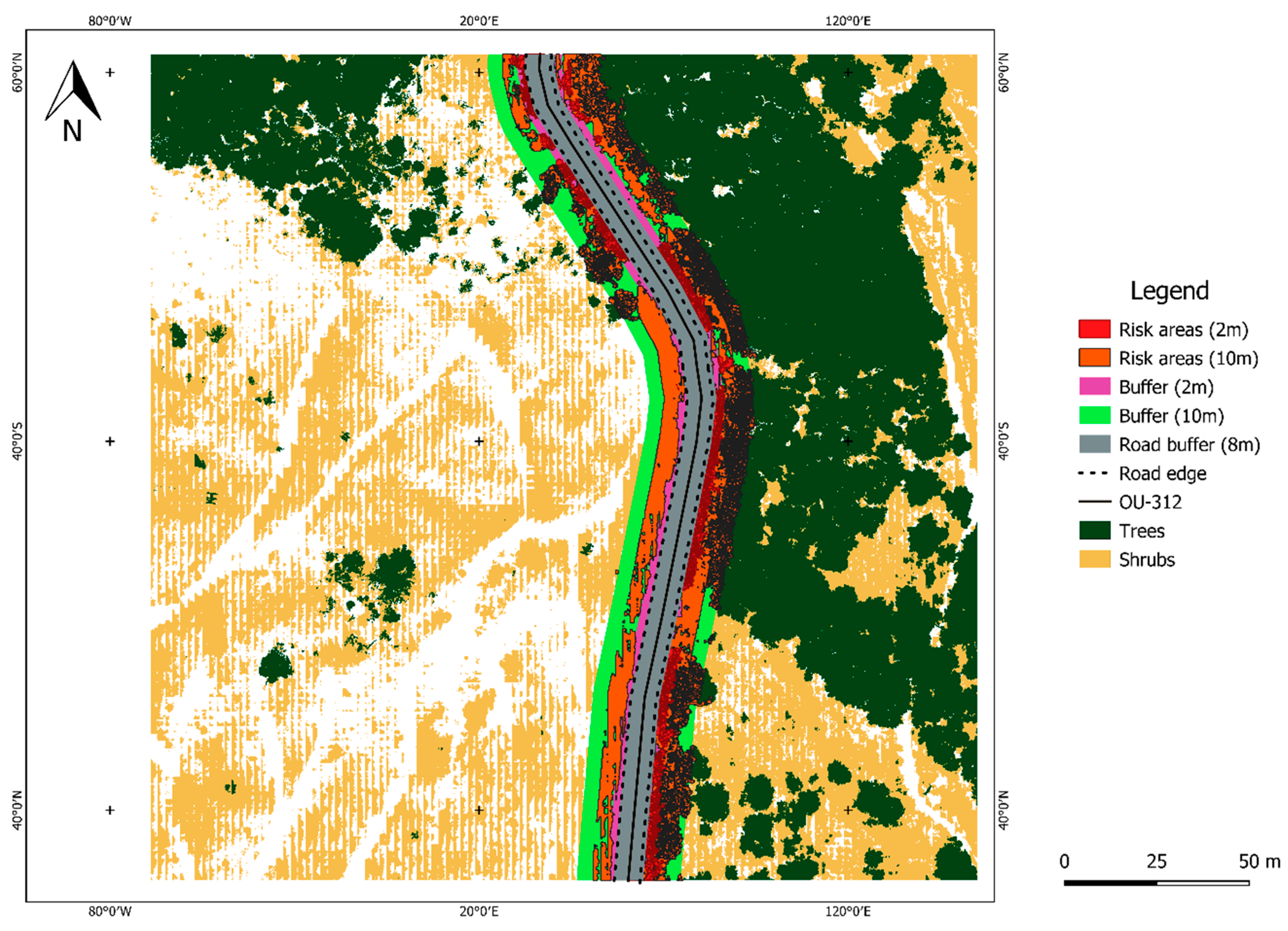
- Identification and surface calculation of potential risk areas of forest fires around the road.
2. Materials and Methods
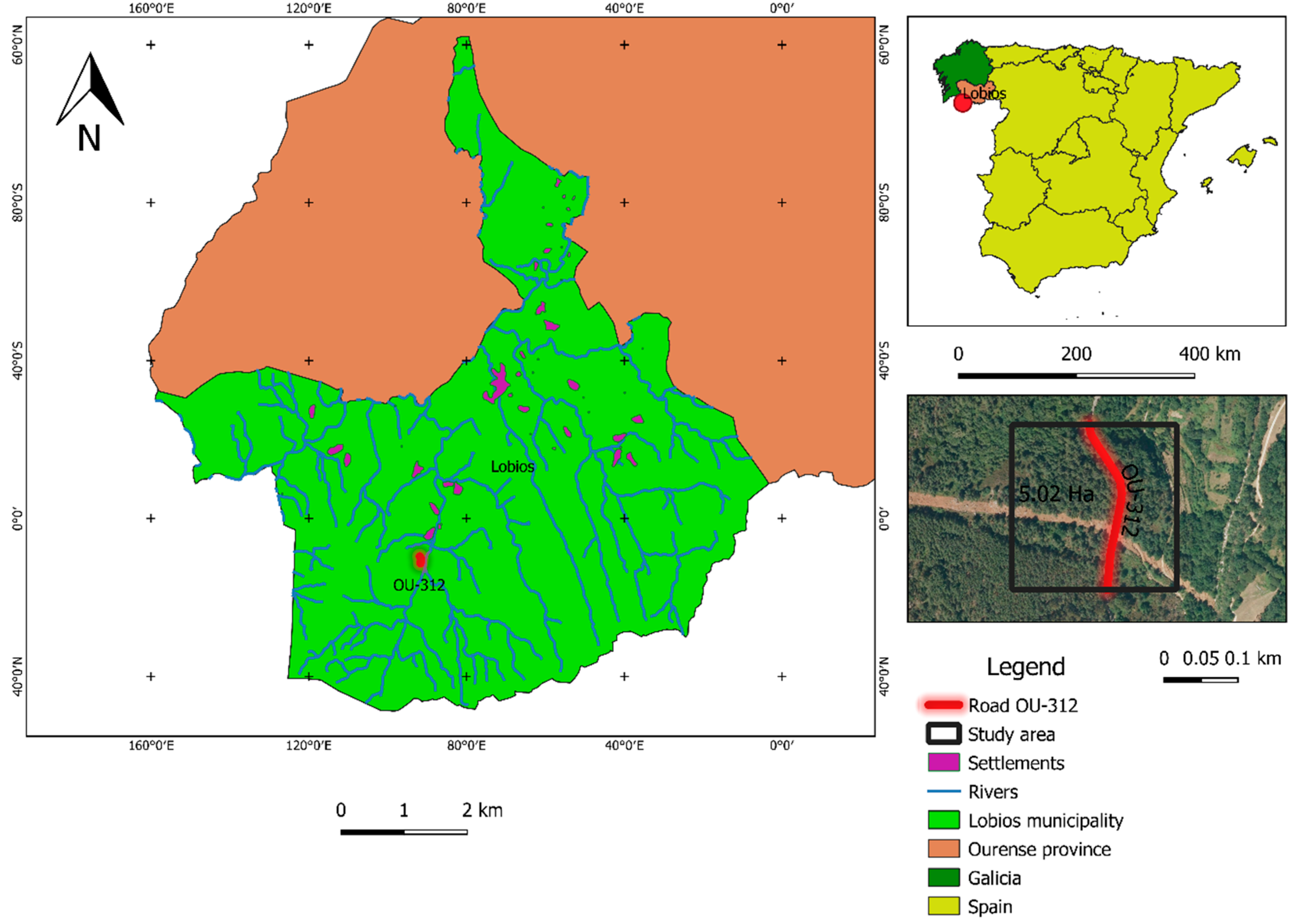
2.1. Area of Study
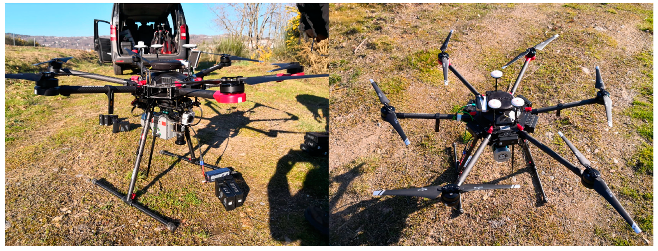
2.2. Aerial LiDAR System
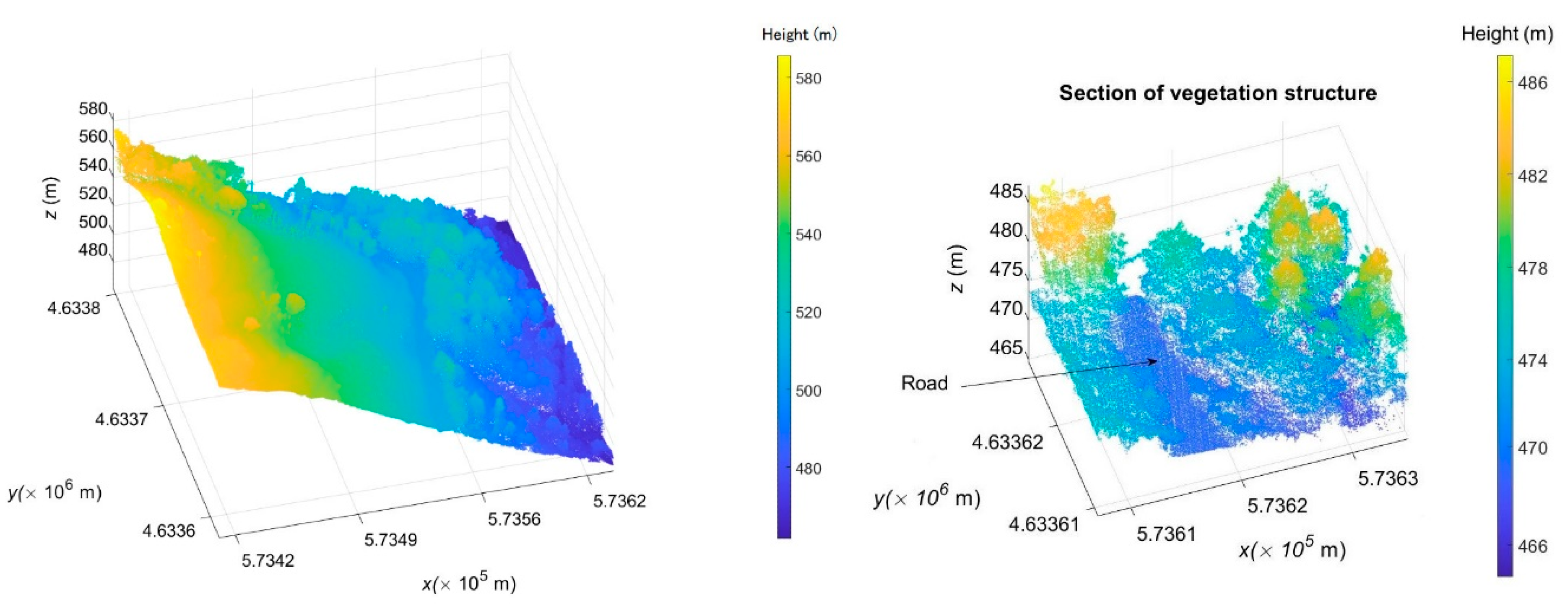
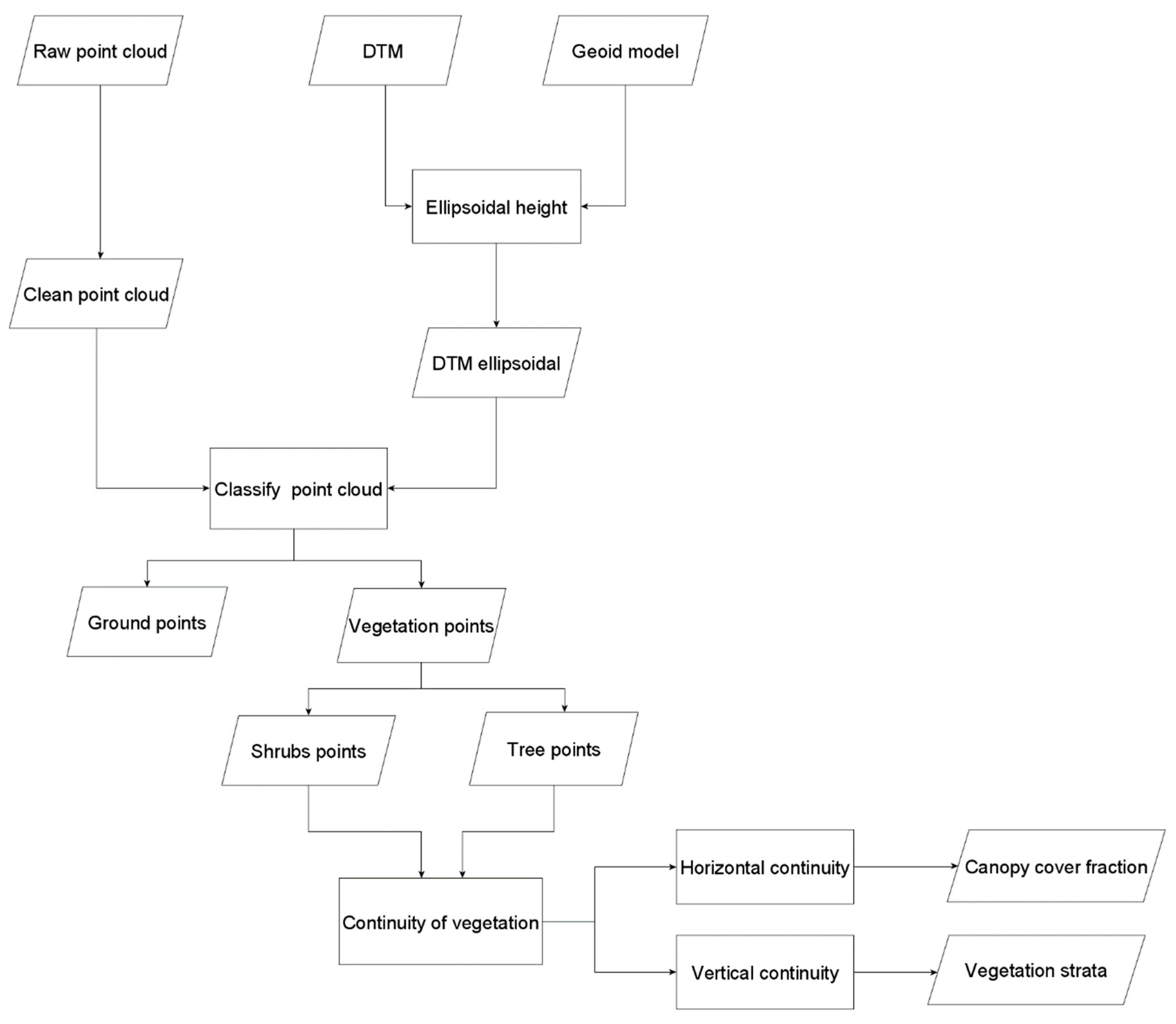
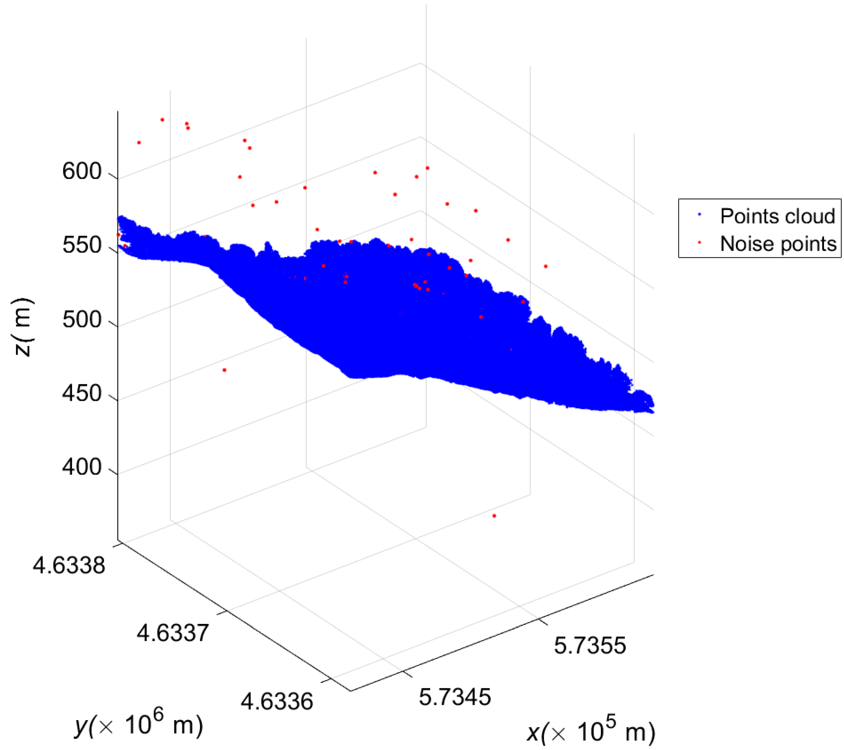
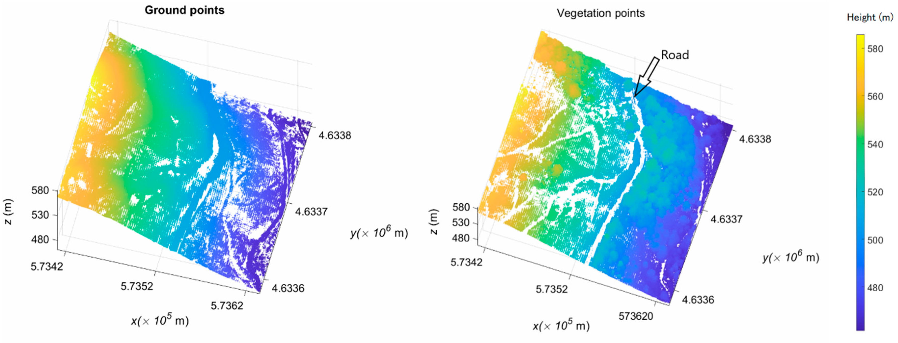
2.3. Data Processing
3. Results
4. Discussion
5. Conclusions
Author Contributions
Funding
Acknowledgments
Conflicts of Interest
References
- Government of Spain Ministerio de Agricultura, Pesca y Educacion. Available online: https://www.mapa.gob.es/ (accessed on 2 March 2020).
- Galicia.Ley 3/2007, de 9 de Abril, de Prevencion y Defensa Contra los Incendios Forestales de Galicia. Boletin Oficial del Estado 119, 18 May 2007; pp. 21377–21394.
- Gucinski, H.; Furniss, M.J.; Ziemer, R.R.; Brookes, M.H. Forest Roads: A Synthesis of Scientific Information; USDA. Forest Service. Pacific Northwest Research Station, General Technical Report PNW-GTR-509; United States Department of Agriculture: Portland, OR, USA, 2001; pp. 1–103.
- Birch, D.S.; Morgan, P.; Kolden, C.A.; Abatzoglou, J.T.; Dillon, G.K.; Hudak, A.T.; Smith, A.M.S. Vegetation, topography and daily weather influenced burn severity in central Idaho and western Montana forests. Ecosphere 2015, 6, 1–23. [Google Scholar] [CrossRef]
- Fang, L.; Yang, J.; Zu, J.; Li, G.; Zhang, J. Quantifying influences and relative importance of fire weather, topography, and vegetation on fire size and fire severity in a Chinese boreal forest landscape. For. Ecol. Manag. 2015, 356, 2–12. [Google Scholar] [CrossRef]
- Jain, T.B.; Graham, R.T. The Relation Between Tree Burn Severity and Forest Structure in the Rocky Mountains; Pacific Southwest Research Station, Forest Service, U.S. Department of Agriculture: Albany, CA, USA, 2007; pp. 213–250.
- Zald, H.S.J.; Dunn, C.J. Severe fire weather and intensive forest management increase fire severity in a multi-ownership landscape. Ecol. Appl. 2018, 28, 1068–1080. [Google Scholar] [CrossRef] [PubMed]
- Haidari, M.; Namiranian, M.; Ghahramany, L.; Zobeiri, M.; Shabanian, N. Study of vertical and horizontal forest structure in Northern Zagros Forest (Case study: West of Iran, Oak forest). Eur. J. Exp. Biol. 2013, 2013, 268–278. [Google Scholar]
- Riaño, D.; Chuvieco, E.; Ustin, S.L.; Salas, J.; Rodríguez-Pérez, J.R.; Ribeiro, L.M.; Viegas, D.X.; Moreno, J.M.; Fernández, H. Estimation of shrub height for fuel-type mapping combining airborne LiDAR and simultaneous color infrared ortho imaging. Int. J. Wildl. Fire 2007, 16, 341–348. [Google Scholar] [CrossRef] [Green Version]
- Chuvieco, E.; Wagtendonk, J.; Riaño, D.; Yebra, M.; Ustin, S.L. Estimation of fuel conditions for fire danger assessment. In Earth Observation of Wildland Fires in Mediterranean Ecosystems; Springer: Berlin/Heidelberg, Germany, 2009; pp. 83–96. [Google Scholar]
- Lim, K.; Treitz, P.; Wulder, M.; St-Onge, B.; Flood, M. LiDAR remote sensing of forest structure. Prog. Phys. Geogr. Earth Environ. 2003, 27, 88–106. [Google Scholar] [CrossRef] [Green Version]
- Andersen, H.-E.; Reutebuch, S.E.; McGaughey, R.J. A rigorous assessment of tree height measurements obtained using airborne lidar and conventional field methods. Can. J. Remote Sens. 2006, 32, 355–366. [Google Scholar] [CrossRef]
- Andresen, C.G.; May, J.A.; Townsend, P.A.; Desai, A.R. Forest canopy structure characterization using high-density UAV LiDAR. AGUFM 2019, 2019, B41K-2505. [Google Scholar]
- Hudak, A.T.; Lefsky, M.A.; Cohen, W.B.; Berterretche, M. Integration of lidar and Landsat ETM+ data for estimating and mapping forest canopy height. Remote Sens. Environ. 2002, 82, 397–416. [Google Scholar] [CrossRef] [Green Version]
- Antonarakis, A.S.; Richards, K.S.; Brasington, J. Object-based land cover classification using airborne LiDAR. Remote Sens. Environ. 2008, 112, 2988–2998. [Google Scholar] [CrossRef]
- Axelsson, P. DEM generation from laser scanner data using adaptive TIN models. Int. Arch. Photogramm. Remote Sens. 2000, 33, 110–117. [Google Scholar]
- Balsi, M.; Esposito, S.; Fallavollita, P.; Nardinocchi, C. Single-tree detection in high-density LiDAR data from UAV-based survey. Eur. J. Remote Sens. 2018, 51, 679–692. [Google Scholar] [CrossRef] [Green Version]
- Baltsavias, E.P. Airborne laser scanning: Basic relations and formulas. ISPRS J. Photogramm. Remote Sens. 1999, 54, 199–214. [Google Scholar] [CrossRef]
- Wang, C.; Glenn, N.F. A linear regression method for tree canopy height estimation using airborne lidar data. Can. J. Remote Sens. 2008, 34, S217–S227. [Google Scholar] [CrossRef]
- Liang, X.; Wang, Y.; Pyörälä, J.; Lehtomäki, M.; Yu, X.; Kaartinen, H.; Kukko, A.; Honkavaara, E.; Issaoui, A.E.I.; Nevalainen, O.; et al. Forest in situ observations using unmanned aerial vehicle as an alternative of terrestrial measurements. For. Ecosyst. 2019, 6, 20. [Google Scholar] [CrossRef] [Green Version]
- Packalén, P.; Pitkänen, J.; Maltamo, M. Comparison of individual tree detection and canopy height distribution approaches: A case study in Finland. In Proceedings of the SilviLaser 2008 8th, Edinburgh, UK, 17–19 September 2008. [Google Scholar]
- Næsset, E.; Bjerknes, K.-O. Estimating tree heights and number of stems in young forest stands using airborne laser scanner data. Remote Sens. Environ. 2001, 78, 328–340. [Google Scholar] [CrossRef]
- Zimble, D.A.; Evans, D.L.; Carlson, G.C.; Parker, R.C.; Grado, S.C.; Gerard, P.D. Characterizing vertical forest structure using small-footprint airborne LiDAR. Remote Sens. Environ. 2003, 87, 171–182. [Google Scholar] [CrossRef] [Green Version]
- Maier, B.; Tiede, D.; Dorren, L. Characterising mountain forest structure using landscape metrics on LiDAR-based canopy surface models. In Object-Based Image Analysis; Springer: Berlin/Heidelberg, Germany, 2008; pp. 625–643. [Google Scholar]
- Pascual, C.; Garcia-Abril, A.; Cohen, W.B.; Martin-Fernandez, S. Relationship between LiDAR-derived forest canopy height and Landsat images. Int. J. Remote Sens. 2010, 31, 1261–1280. [Google Scholar] [CrossRef]
- Hermosilla, T.; Ruiz, L.A.; Kazakova, A.N.; Coops, N.C.; Moskal, L.M. Estimation of forest structure and canopy fuel parameters from small-footprint full-waveform LiDAR data. Int. J. Wildl. Fire 2014, 23, 224–233. [Google Scholar] [CrossRef] [Green Version]
- Kane, V.R.; North, M.P.; Lutz, J.A.; Churchill, D.J.; Roberts, S.L.; Smith, D.F.; McGaughey, R.J.; Kane, J.T.; Brooks, M.L. Assessing fire effects on forest spatial structure using a fusion of Landsat and airborne LiDAR data in Yosemite National Park. Remote Sens. Environ. 2014, 151, 89–101. [Google Scholar] [CrossRef]
- Marino, E.; Montes, F.; Tomé, J.L.; Navarro, J.A.; Hernando, C. Vertical forest structure analysis for wildfire prevention: Comparing airborne laser scanning data and stereoscopic hemispherical images. Int. J. Appl. Earth Obs. Geoinf. 2018, 73, 438–449. [Google Scholar] [CrossRef]
- Xunta de Galicia. Available online: http://mediorural.xunta.gal/es/areas/forestal/ordenacion/distritos/ (accessed on 23 March 2020).
- QGIS. Available online: https://www.qgis.org/es/site/ (accessed on 23 March 2020).
- Van Rossum, G. Python Programming Language. In Proceedings of the USENIX Annual Technical Conference, Santa Clara, CA, USA, 17–22 June 2007; Volume 41, p. 36. [Google Scholar]
- CNIG Centro Nacional de Información Geográfica. Available online: http://centrodedescargas.cnig.es/CentroDescargas/index.jsp (accessed on 16 March 2020).
- Ruchay, A.N.; Dorofeev, K.A.; Kalschikov, V.V. Accuracy analysis of 3D object reconstruction using point cloud filtering algorithms. In Proceedings of the 5th Information Technology and Nanotechnology 2019: Image Processing and Earth Remote Sensing, ITNT 2019, Samara, Russia, 21–24 May 2019; Volume 2391, pp. 169–174. [Google Scholar]
- Marino, E.; Ranz, P.; Tomé, J.L.; Noriega, M.Á.; Esteban, J.; Madrigal, J. Generation of high-resolution fuel model maps from discrete airborne laser scanner and Landsat-8 OLI: A low-cost and highly updated methodology for large areas. Remote Sens. Environ. 2016, 187, 267–280. [Google Scholar] [CrossRef]
- García, M.; Riaño, D.; Chuvieco, E.; Salas, J.; Danson, F.M. Multispectral and LiDAR data fusion for fuel type mapping using Support Vector Machine and decision rules. Remote Sens. Environ. 2011, 115, 1369–1379. [Google Scholar] [CrossRef]
- Price, O.F.; Gordon, C.E. The potential for LiDAR technology to map fire fuel hazard over large areas of Australian forest. J. Environ. Manag. 2016, 181, 663–673. [Google Scholar] [CrossRef]
- Mitchell, J.J.; Glenn, N.F.; Sankey, T.T.; Derryberry, D.R.; Anderson, M.O.; Hruska, R.C. Small-footprint LiDAR estimations of sagebrush canopy characteristics. Photogramm. Eng. Remote Sens. 2011, 77, 521–530. [Google Scholar] [CrossRef]
- Novo, A.; González-Jorge, H.; Martínez-Sánchez, J.; Lorenzo, H. Canopy detection over roads using mobile lidar data. Int. J. Remote Sens. 2020, 41, 1927–1942. [Google Scholar] [CrossRef]
- Otsu, N. A threshold selection method from gray-level histograms. IEEE Trans. Syst. Man Cybern. 1979, 9, 62–66. [Google Scholar] [CrossRef] [Green Version]


© 2020 by the authors. Licensee MDPI, Basel, Switzerland. This article is an open access article distributed under the terms and conditions of the Creative Commons Attribution (CC BY) license (http://creativecommons.org/licenses/by/4.0/).
Share and Cite
Novo, A.; Fariñas-Álvarez, N.; Martínez-Sánchez, J.; González-Jorge, H.; Lorenzo, H. Automatic Processing of Aerial LiDAR Data to Detect Vegetation Continuity in the Surroundings of Roads. Remote Sens. 2020, 12, 1677. https://0-doi-org.brum.beds.ac.uk/10.3390/rs12101677
Novo A, Fariñas-Álvarez N, Martínez-Sánchez J, González-Jorge H, Lorenzo H. Automatic Processing of Aerial LiDAR Data to Detect Vegetation Continuity in the Surroundings of Roads. Remote Sensing. 2020; 12(10):1677. https://0-doi-org.brum.beds.ac.uk/10.3390/rs12101677
Chicago/Turabian StyleNovo, Ana, Noelia Fariñas-Álvarez, Joaquin Martínez-Sánchez, Higinio González-Jorge, and Henrique Lorenzo. 2020. "Automatic Processing of Aerial LiDAR Data to Detect Vegetation Continuity in the Surroundings of Roads" Remote Sensing 12, no. 10: 1677. https://0-doi-org.brum.beds.ac.uk/10.3390/rs12101677