Performance Evaluation of the Multiple Quantile Regression Model for Estimating Spatial Soil Moisture after Filtering Soil Moisture Outliers

Abstract

The spatial distribution of soil moisture (SM) was estimated by a multiple quantile regression (MQR) model with Terra Moderate Resolution Imaging Spectroradiometer (MODIS) and filtered SM data from 2013 to 2015 in South Korea. For input data, observed precipitation and SM data were collected from the Korea Meteorological Administration and various institutions monitoring SM. To improve the work of a previous study, prior to the estimation of SM, outlier detection using the isolation forest (IF) algorithm was applied to the observed SM data. The original observed SM data resulted in IF_SM data following outlier detection. This study obtained an average data removal rate of 20.1% at 58 stations. For various reasons, such as instrumentation, environment, and random errors, the original observed SM data contained approximately 20% uncertain data. After outlier detection, this study performed a regression analysis by estimating land surface temperature quantiles. The soil characteristics were considered through reclassification into four soil types (clay, loam, silt, and sand), and the five-day antecedent precipitation was considered in order to estimate the regression coefficient of the MQR model. For all soil types, the coefficient of determination (R²) and root mean square error (RMSE) values ranged from 0.25 to 0.77 and 1.86% to 12.21%, respectively. The MQR results showed a much better performance than that of the multiple linear regression (MLR) results, which yielded R² and RMSE values of 0.20 to 0.66 and 1.08% to 7.23%, respectively. As a further illustration of improvement, the box plots of the MQR SM were closer to those of the observed SM than those of the MLR SM. This result indicates that the cumulative distribution functions (CDF) of MQR SM matched the CDF of the observed SM. Thus, the MQR algorithm with outlier detection can overcome the limitations of the MLR algorithm by reducing both the bias and variance.

1. Introduction

To understand hydrological processes, including evapotranspiration, infiltration, percolation, and runoff, soil moisture (SM) is a key variable [1]. Therefore, understanding the spatial distribution of SM is crucial in analyzing hydrological processes [2]. In addition to using water resources research to study rainfall runoff, SM has been widely used in other specific fields, such as in agriculture to study plant growth and hydrometeorology to study interactions between the atmosphere and land [3]. In the past, SM data were obtained by measuring in the laboratory by soil sample analysis or in the field by in situ SM probes at the temporal scales of every day to biweekly using various field techniques, such as capacitance measurements and time/frequency domain reflectometry (TDR/FDR). TDR involves an electronic instrument used to capture representative soil water content measurements. However, these methods have limitations in that it is difficult to obtain representative SM data over a large area due to the point-based nature of such measurements [4], and that such methods are expensive when applied to large areas. To overcome these shortcomings, many studies have continued to estimate the spatial SM distribution using satellite data [5].

There are two broad categories of remote sensing methods used to estimate spatial SM periodically: indirect measurements based on land surface parameters and direct measurements using microwave satellites. First, satellites with microwave sensors produce SM estimates by using surface variables such as backscatter and brightness temperature [6,7,8,9,10,11,12,13]. Microwave satellites can provide daily SM data at a global scale with a low frequency and resolution [14,15,16]. Therefore, such methods are commonly deemed to be appropriate for uses on a global scale [17,18]. Despite these advantages, it remains difficult to monitor local-scale SM estimates and droughts [19]. Additionally, local or regional applications related to the fields of agricultural and hydrology remain challenging because of these difficulties [20,21,22]. Second, the spatial distribution of SM can be estimated by regression analysis using various variables, such as the normalized difference vegetation index (NDVI) and the land surface temperature (LST), without using microwave satellite data [4]. Although the spatial SM was estimated based on LST data and multiple linear regression (MLR) analysis in a previous study [5], simple linear regression analysis algorithms do not fully explain the behavior of SM, which varies in response to weather, season, and soil type. Moreover, in the previous study, the soil properties were reclassified into four classes and subjected to regression analysis to compensate for the limitations of insufficient SM observation data. In this reclassification process, there was a possibility that many uncertainties would appear in the SM data. Thus, to reduce uncertainty and to improve the research results of SM behavior tracking, it has become necessary to develop an algorithm to remove outliers in SM input data.

Since LST shows varying sensitivity to vegetation and soil, a direct relationship between LST and SM has not been clearly identified [23], although LST is one of the essential elements for estimating SM [24,25]. Originally, a unique relationship between spatial SM and LST was proposed by previous studies [26,27,28,29] and many studies have been conducted utilizing this relationship [30,31,32,33,34]. Although LST data from the Moderate Resolution Imaging Spectroradiometer (MODIS) has been applied to indirectly calculate the SM content, prior to using indirect data, noise caused by various factors from all indirect satellite data should be eliminated through preprocessing, such as gap filling and interpolation [5]. By applying one of these methods, previous studies have shown that MODIS LST can be reconstructed by geostatistical interpolations considering spatiotemporal properties [35,36]. These geostatistical interpolations, such as spline methods, kriging, inverse distance weighting (IDW), and conditional merging (CM) have been used for correction by matching satellite data and ground-measured data at various spatial scales [37,38]. These geostatistical methods have been widely used for combining satellite-based and observational data. Moreover, the CM method has been used in research related to radar observation to correct the error that may occur in the original kriging method [39]. Additionally, Jung et al. [5] applied the CM method to correct LST data, which yielded a better spatiotemporal distribution than that of the original LST data.

In this study, the spatial distribution of SM was estimated via the multiple quantile regression (MQR) method based on MODIS NDVI and LST data (Figure 1), and the procedure is as follows: (1) outliers in the observed SM were removed using the isolation forest (IF) algorithm, (2) the spatial distribution error of MODIS LST was modified by applying the CM method, (3) the spatial distribution of SM was estimated through the MQR model development, and (4) the applicability of the model was evaluated. Finally, the results of this study were compared with those of a previous study [5], in which the SM was calculated by the MLR model, to show the improvement.

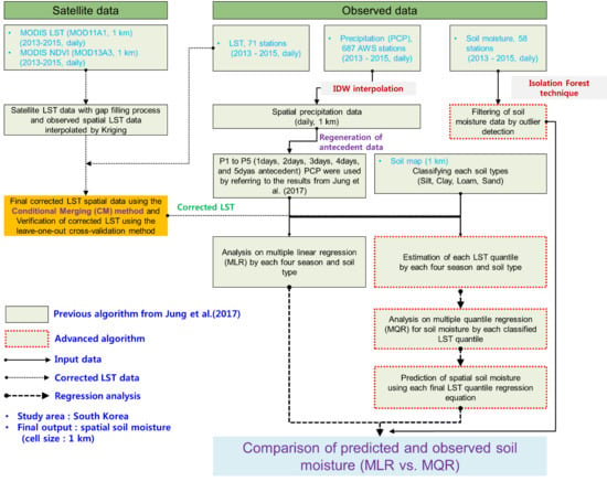
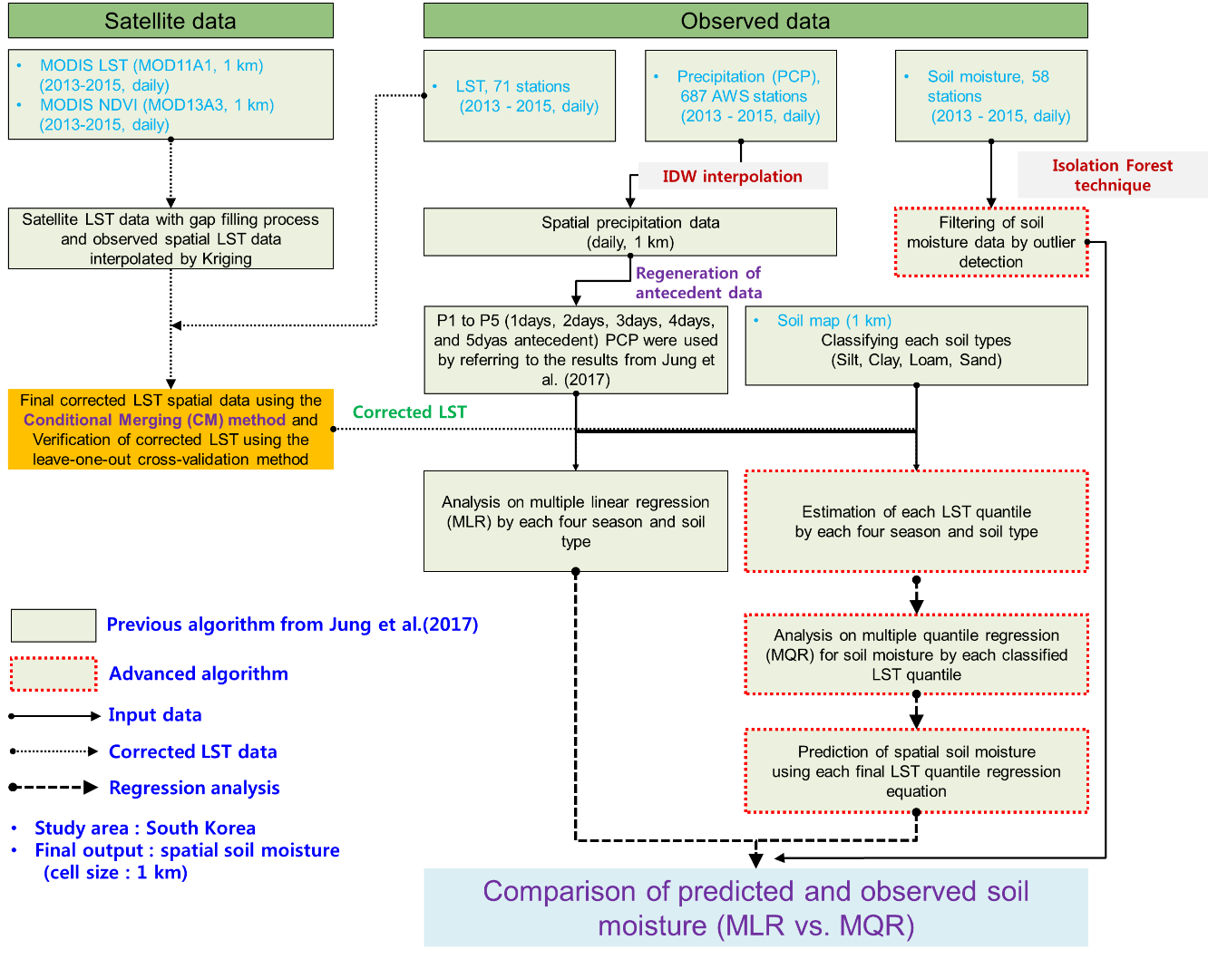
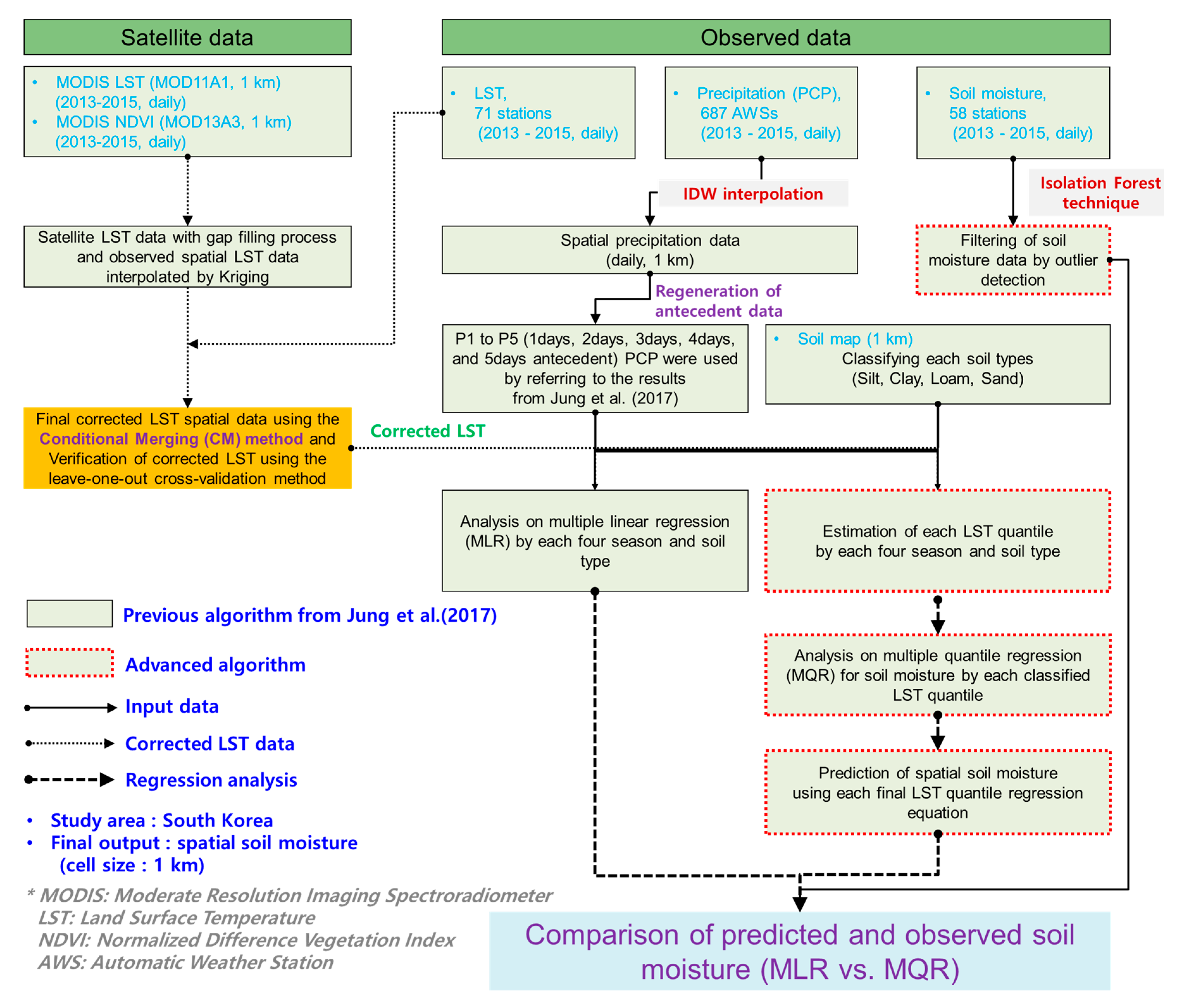
2. Materials and Methods

MQR was the main algorithm used in this study, and it is important because it can handle many types of data. In a previous study [5], input data, such as MODIS LST, NDVI, and precipitation, were selected for estimating SM using principal component analysis. A soil map for obtaining soil properties, wilting point, and field capacity was prepared from data provided by the Korea Rural Development Administration (KRDA). All spatial data, such as satellite data and soil maps, were prepared with a spatial resolution of 1 km, and observed data, such as precipitation and SM, were prepared with the same spatial resolution using the IDW technique [40].

2.1. MODIS Data

The MODIS data were prepared from the Land Processes Distributed Active Archive Center (LP DAAC, https://lpdaac.usgs.gov/) and EARTHDATA (https://earthdata.nasa.gov/), including MODIS LST (MOD11A1) and vegetation indices (MOD13Q1). The MOD11A1 provided daily per-pixel LST in Kelvin at a 1 km spatial resolution, and low-quality pixels, such as those with clouds and other atmospheric disturbances, were marked in an accompanying quality assessment (QA) layer. These pixels were corrected and reconstructed by the CM method. The advantage of this method is that it can preserve the spatial distribution, maintaining the precision of the observed data. In a previous study [5], high-precision LST data were estimated through the application of this method, and the corrected LST data were also used in this study. Please refer to the previous paper [5] for detailed methods and procedures for generating the corrected LST data.

The MODIS vegetation product (MOD13Q1) provides temporally and spatially continuous NDVI data with a 16-day interval at 250 m resolution from January 2013 to May 2015. Normally, when calculating daily SM through regression analysis, daily input data are required, but daily NDVI data were not available. Although vegetation changes vary by type of vegetation, vegetation generally becomes more vigorous from spring to summer and gradually fades from autumn to winter. In addition, rapid changes are not common in forests. Therefore, in this study, NDVI data with a 16-day interval were applied as the vegetation data for daily SM estimation, and the spatial resolution was resampled to 1000 m, which is the same as the LST data.

2.2. Observed Data

In South Korea, the Korea Meteorological Administration (KMA) is constructing a high-density ground observation network through the establishment of 687 automatic weather stations (AWSs, Figure 2a). AWSs monitor weather data, such as precipitation, wind speed, and humidity, on the order of minutes, which produce data with a much higher accuracy than satellite data. The precipitation data acquired from AWSs were interpolated to a 1 km spatial resolution, the same as the MODIS data. The SM observation data were obtained from 58 stations run by various institutions (

Table 1. Soil moisture stations with soil type.

No.	Station	Class	No.	Station	Class	No.	Station	Class	No.	Station	Class
1	CW	Sand	16	PU	Loam	31	NI	Clay	46	SD2	Loam
2	SW	Sand	17	HH2	Clay	32	JJ4	Clay	47	SC2	Clay
3	SC1	Sand	18	II	Loam	33	JJ5	Clay	48	YY3	Silt
4	CJ	Sand	19	CH	Loam	34	YG2	Clay	49	CC4	Sand
5	CC1	Clay	20	CO	Clay	35	GO	Loam	50	YO	Clay
6	SS1	Clay	21	YS2	Silt	36	HH4	Clay	51	PB	Loam
7	BS	Sand	22	JB	Sand	37	HH5	Clay	52	GG4	Silt
8	CC2	Loam	23	NG	Clay	38	YD	Clay	53	TG2	Silt
9	GB1	Silt	24	GD	Loam	39	HS	Clay	54	JC2	Clay
10	JC1	Loam	25	YS3	Silt	40	HU	Clay	55	SY	Clay
11	HB	Loam	26	CC3	Loam	41	JG	Clay	56	HJ	Clay
12	YC	Loam	27	HH3	Clay	42	BU	Silt	57	GG5	Loam
13	IJ	Silt	28	JJ3	Loam	43	YJ	Clay	58	HH6	Sand
14	YY1	Loam	29	GB2	Clay	44	GJ	Clay
15	HH1	Clay	30	MM	Clay	45	CY	Clay

). Stations 1 to 9 were from the Automated Agriculture Observing System (AAOS) of the KMA. Stations 10 and 11 were from the Korea Institute of Hydrological Survey (KIHS), and stations 13 to 18 were from K-water. The other stations were from the Rural Development Administration (RDA).

The soil map, which includes information on the field capacity, wilting point, and soil types, was essential for estimating SM. The SM map supplied by the RDA was sorted into 12 classes according to the U.S. Department of Agriculture (USDA) textural classification. However, due to the limitation of insufficient data with no minimum data for estimating the regression coefficient according to the 12 soil types, the soil types were reclassified into silt, clay, loam, and sand, based on the soil textural triangle. Sand represents sand, sandy loam, and loamy sand in the triangle. Likewise, clay represents silty clay, sandy clay, silty clay loam, and clay, and loam represents loam, clay loam, and sandy clay loam. Finally, silt represents silty loam and silt [16]. Figure 2b show the soil information at the SM stations. Of the 58 SM stations, clay accounts for approximately 48% (28 stations), and loam accounts for approximately 24% (14 stations). Therefore, considerable data are available for two soil types (clay and loam). Furthermore, in this study, the IF algorithm, which eliminates outliers, was applied to solve the uncertainty that can occur while reclassifying the soil texture into four classes. This process represents a quality control (QC) process for original SM data to which no QC processes have been applied.

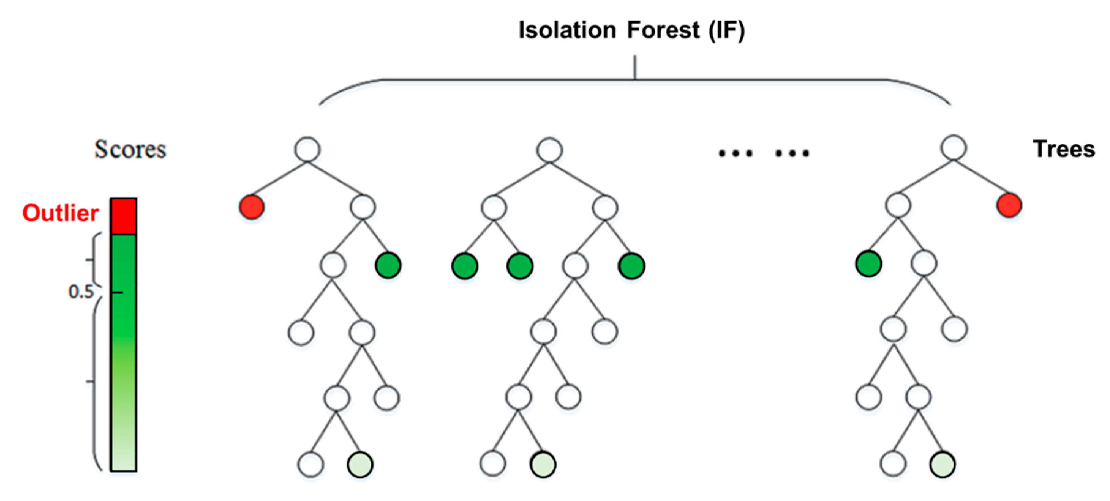
2.3. Anomaly Detection Algorithm

Outlier detection, or anomaly detection, is a method to find the patterns in datasets that do not match expected patterns that differ significantly from it. There are a variety of methods such as isolation-based method, modal-based method, density-based method, and distance-based method. Among them, IF is an effective technique using a machine learning algorithm based on binary tree structures with a random sampling method that provides an ensemble of a series of trees from multidimensional training and testing data sets. Compared to other anomaly detection algorithms, the reasons for adopting IF in this study are as follows: (1) building iTrees is relatively straightforward, as users only need to randomly select a subset of the training sets; (2) it takes less time to calculate since it does not measure distance or density; (3) low memory requirements; and (4) the ensemble algorithm can overcome the low efficiency of iTrees [41]. The basic concept of IF is that the few anomalous data far from the normal cluster center can be identified through anomaly detection [42]. The IF technique consists of a two-stage procedure. A training step structures basic isolation trees that build various subsamples using random sampling from the training set. The testing step calculates the length of the path by passing samples to obtain an anomaly score through isolation trees (Figure 3).

To isolate every subsample and stage, a tree structure can be used effectively because there are few anomalies far from normal points. While normal samples can be far from the root, anomalies are closer to the root of the tree. Between the minimum and maximum values of the attribute, partitions of every IF structure are selected at random, and automatically recursive partitions are passed. A randomly selected partition is calculated, and each tree is classified by dividing different structures. Finally, each path length is calculated to determine an outlier score. The definition of the anomaly score for instance x is:

$$\mathrm{s}\left(x,n\right)=2^{-\frac{E\left(h\left(x\right)\right)}{c\left(n\right)}}$$

(1)

$$\mathrm{c}\left(\mathrm{n}\right)=2H\left(n-1\right)-\left(\frac{2\left(n-1\right)}{n}\right)$$

(2)

where $H\left(i\right)$ can be estimated by $\ln \left(i\right)+0.5772156649$ (Euler’s constant) as the harmonic number since c(n) is the constant value to normalize the average path length for n trees. $n$ is the number of nodes ($n$). $h\left(x\right)$ is the path length of sample $x$ by the number of edges x traverses and iTrees from the root node until the traversal is terminated at an external node. $E\left(h\left(x\right)\right)$ is the average path length of each $h\left(x\right)$ from a collection of iTrees. $s$ is the anomaly score used in the following evaluation. The evaluation includes the following processes: (a) if $s$ is very close to 1, then it is clearly an anomaly; and (b) if $\mathrm{s}$ is much smaller than 0.5, then it may truly be a normal point. For instance, when s is 1, $E\left(h\left(x\right)\right)$ will be zero (0). This means that all the path length for all n trees get close to the root node. In this study, the IF structure consisted of the sklearn-ensemble library in Python.

To confirm that the IF outlier detection technique really removed the uncertainty of the SM data, this study suggested a data removal rate (DRR) and the percentage of matching SM increases with increasing precipitation (PCP), which is COR_PCP, to assess tendency showing SM increases with increasing PCP at the same time. Two indicators are as following Equations (3) and (4):

$$\mathrm{DRR}(\%)=\frac{\left(\mathrm{Number}\mathrm{of}\mathrm{raw}\mathrm{data}\right)-\left(\mathrm{Number}\mathrm{of}\mathrm{IF}\_\mathrm{SM}\right)}{\left(\mathrm{Number}\mathrm{of}\mathrm{raw}\mathrm{data}\right)}\times 100$$

(3)

$$\mathrm{COR}\_\mathrm{PCP}(\%)=\frac{\left(\mathrm{Number}\mathrm{of}\mathrm{days}\mathrm{matching}\mathrm{SM}\mathrm{increases}\mathrm{with}\mathrm{increasing}\mathrm{PCP}\mathrm{at}\mathrm{the}\mathrm{same}\mathrm{time}\right)}{\left(\mathrm{Number}\mathrm{of}\mathrm{the}\mathrm{rainfall}\mathrm{days}\right)}\times 100$$

(4)

2.4. Multiple Quantile Regression Model

It is possible to estimate the conditional quartile by considering various quantiles for the dependent variable as the parametric method. In addition, this method can be applied to a case where the distribution of the given data is large or heterogeneous [43]. In addition, since the influence of dependent variables according to independent variables can be estimated in various quartiles, it is possible to perform regression analysis considering the distribution characteristics of time series so that it is not only superior in methodology but also easy to expand to nonlinear models [44].

Quantile regression analysis can directly evaluate LST trends as a method for determining the linear and nonlinear trends of a particular quantile (r) in the overall data. This trend is expressed by the following equation [45]:

$$y_r=\min \{{{\displaystyle \sum }}_{\left\{i\right|y_i<y_r\left(x_i\right)\}}\left(1-r\right)\left|y_i-y_r\left(x_i\right)\right|+{{\displaystyle \sum }}_{\left\{i|y_i>y_r\left(x_i\right)\right\}}r\left|y_i-y_r\left(x_i\right)\right|\}$$

(5)

where i denotes the i-th value among the n data, i = 1, 2, …, n. As seen from the above equation, the regression analysis of the min-squared regression assesses the tendency to minimize the sum of the errors of the weights multiplied by the weight line r based on the trend line of the r values. The method of finding the trend line is similar to the least-squares method, but it differs in that it uses the sum of absolute values instead of the sum of squared errors. In this way, when the absolute value is used instead of the square of the error, the effect of the outliers is less reflected in the process of obtaining the trend equation, so that it is possible to reduce the effect of excessively increasing or decreasing the trend due to the outliers.

MODIS LST, NDVI, and precipitation, including antecedent precipitation from one to five days, were used to develop the MQR model as input data, and regression coefficients and equations were estimated seasonally, which were divided into spring, summer, autumn, and winter. Jung et al. [5] described the process of regression coefficients for suitability of the coefficients, such as p-value and multicollinearity. To predict the spatial distribution of SM, the MQR model was performed by using the LST variable quintiles, including 0.05, 0.1, 0.15, 0.2, 0.25, 0.3, 0.35, 0.4, 0.45, 0.5, 0.55, 0.6, 0.65, 0.7, 0.75, 0.8, 0.85, 0.9, and 0.95, as the single parameter with the greatest correlation with SM among the land surface factors.

3. Results

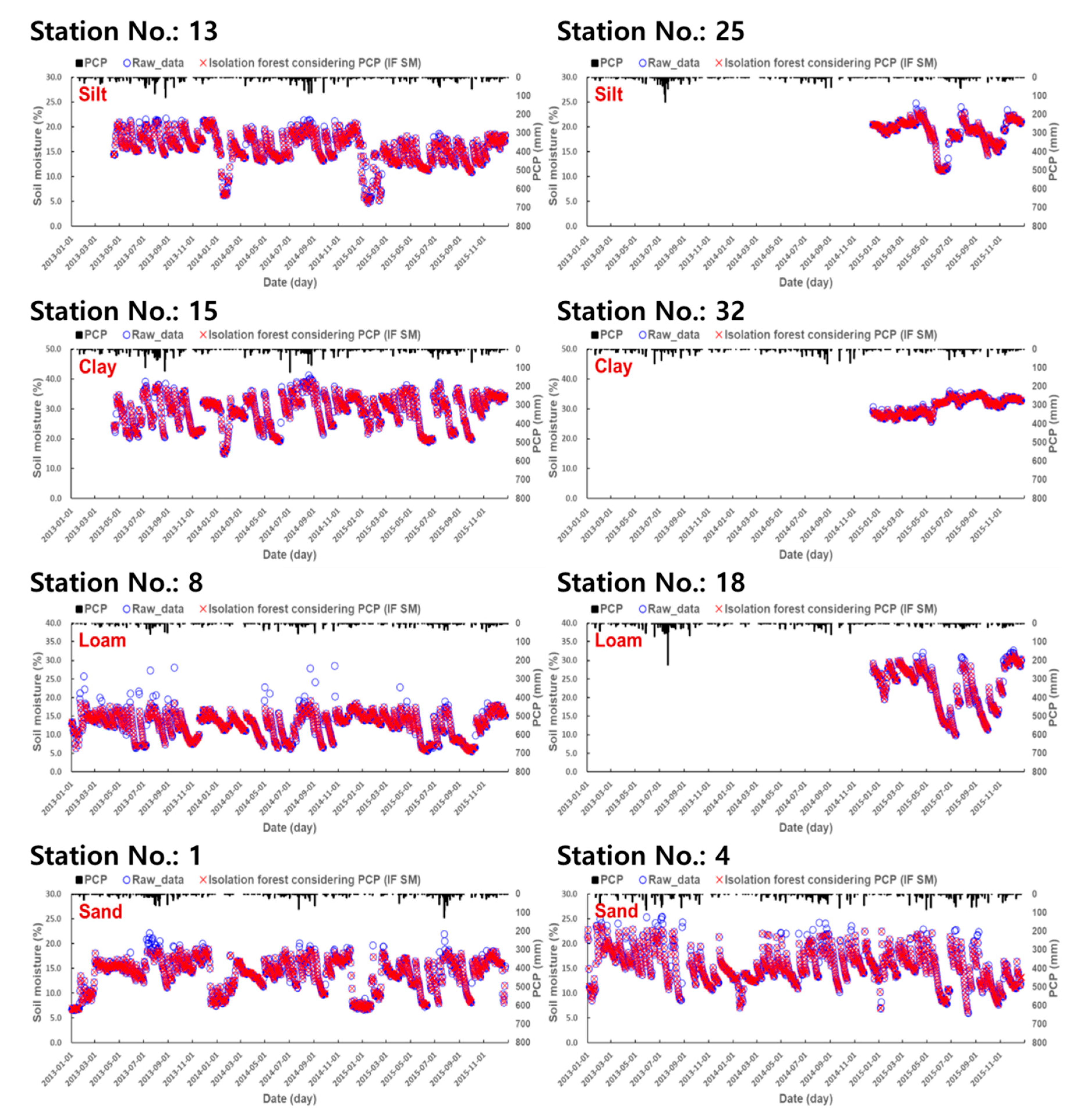
3.1. Outlier Detection of Observed SM Data

To assess tendency showing SM increases with increasing PCP at the same time, the IF developed two algorithms. The first one is the algorithm (IF1) using only observed SM data, and the other one is the algorithm (IF2) using both observed SM data and PCP as an independent variable. Finally, the observed SM data, after applying the IF algorithm for outlier detection (IF_SM), were used as the target variable for quantile regression analysis.

Table 2. Summary of the data removal rate (DRR) and COR_PCP values at 58 soil moisture stations.

Station No.	DRR (%)		COR_PCP (%)		Station No.	DRR (%)		COR_PCP (%)		Station No.	DRR (%)		COR_PCP (%)
	IF1	IF2	IF1	IF2		IF1	IF2	IF1	IF2		IF1	IF2	IF1	IF2
1	9.3	9.4	70.1	74.6	21	28.8	15.7	11.2	23.1	41	28.8	19.1	18.7	28.4
2	10.0	10.0	46.3	62.5	22	28.5	16.2	11.3	19.0	42	28.8	14.9	18.8	30.3
3	9.1	9.1	62.5	69.4	23	28.9	15.0	12.3	23.2	43	28.8	17.3	20.1	25.0
4	8.3	8.3	56.9	68.6	24	30.6	19.2	22.6	25.3	44	28.8	18.1	24.5	31.1
5	10.0	10.0	66.2	73.9	25	28.8	17.3	20.5	29.1	45	28.8	13.9	25.5	32.9
6	9.9	9.9	61.0	75.2	26	29.1	19.3	17.6	21.3	46	28.5	16.0	27.3	28.6
7	9.1	9.1	75.8	75.0	27	29.3	17.6	22.5	26.8	47	28.8	15.2	25.2	29.6
8	10.0	10.0	70.1	82.5	28	28.9	16.8	16.6	22.8	48	28.8	14.7	24.8	32.5
9	10.0	10.0	52.7	66.7	29	28.8	17.3	17.0	21.8	49	28.8	14.9	20.1	30.6
10	21.7	13.3	22.7	31.8	30	28.9	15.0	14.8	24.4	50	30.6	16.4	12.6	24.4
11	2.1	7.6	64.2	64.2	31	28.8	15.7	15.2	26.1	51	28.8	14.4	26.0	33.6
12	7.0	8.3	72.0	73.2	32	28.9	18.9	17.4	26.5	52	28.8	17.5	20.0	24.8
13	1.1	8.2	69.5	72.0	33	28.8	16.5	19.0	22.6	53	28.8	13.6	19.7	28.9
14	1.9	7.8	75.7	71.6	34	30.6	20.6	23.6	31.5	54	28.8	14.7	18.8	28.9
15	1.1	7.6	63.7	70.8	35	28.8	17.0	18.1	25.2	55	30.9	14.6	15.4	25.5
16	28.8	15.7	22.8	30.7	36	28.8	16.8	20.6	27.5	56	28.8	14.1	15.9	24.5
17	29.2	14.1	18.9	28.3	37	28.8	16.2	12.1	24.2	57	28.8	13.6	18.6	27.1
18	28.8	14.1	18.0	29.7	38	28.8	17.0	17.0	25.5	58	28.8	15.7	17.7	25.0
19	28.8	13.6	17.4	25.7	39	28.8	18.6	13.2	23.0
20	28.8	17.8	14.4	26.1	40	28.8	16.5	24.3	29.7

Note: DRR: data removal rate; COR_PCP: tendency showing SM increases with increasing PCP; IF1: isolation forest using only observed SM data; and IF2: isolation forest using both observed SM data and PCP.

shows DRR and COR_PCP at 58 stations. From that result, the average DRR for IF1 and IF2 was 23.6% and 16.0%, respectively. However, the result of IF1 showed that most of the original SM data had approximately 28.8% uncertain data, whereas the result of IF2 showed a variety of removal efficiency. This would come from considering PCP trends. To confirm the basic idea based on increasing SM with increasing PCP, this study applied for IF2 algorithm and compared that using COR_PCP. The COR_PCP showed 26.8% for IF1 and 35.2% for IF2. The results in the IF2 algorithm improved tendency to increasing PCP and SM by about 8.4%. Finally, this study selected the results of the IF2 algorithm. In Figure 4, the raw data (original observed SM) and the isolation forest considering PCP (IF_SM) data were compared at major stations and are illustrated in Figure 4, represented by different marks such as blue circles and red Xs.

3.2. Seasonal Multiple Quantile Regression (MQR) Results

Table 3. Seasonal multiple quantile regression (MQR) regression coefficients according to soil properties.

Class	Season	QT	Con.	NDVI	LST	Precipitation (mm)						R2
						n	n-1	n-2	n-3	n-4	n-5
Silt	Spring	0.1	15.088	0.055	−0.087	0.089	0.079	0.078	0.058	0.066	−3.376	0.39
		0.5	24.553	0.106	−0.106	0.142	0.119	0.104	0.087	0.096	0.719	0.40
		0.9	35.656	0.052	−0.001	0.104	0.046	0.028	0.025	0.030	−9.066	0.41
	Summer	0.1	10.026	0.038	−0.155	0.038	0.027	0.036	0.016	0.021	6.791	0.38
		0.5	17.717	0.058	−0.051	0.055	0.048	0.043	0.043	0.047	6.966	0.40
		0.9	31.081	0.071	0.019	0.058	0.021	0.016	0.029	0.031	−2.576	0.40
	Autumn	0.1	18.406	0.007	−0.100	0.042	0.021	0.017	0.019	0.010	−7.386	0.40
		0.5	22.940	0.065	−0.167	0.079	0.061	0.045	0.026	0.036	5.807	0.37
		0.9	36.441	0.056	−0.045	0.094	0.049	0.030	0.021	−0.001	−8.570	0.41
	Winter	0.1	11.860	0.129	1.008	0.251	0.326	0.235	0.223	0.190	−6.306	0.47
		0.5	25.117	−0.064	0.968	0.090	0.113	0.071	0.108	0.155	−7.171	0.43
		0.9	37.093	−0.034	0.190	0.176	0.068	0.035	0.064	0.059	−15.736	0.42
Clay	Spring	0.1	30.384	0.117	0.059	0.087	0.070	0.046	0.143	0.077	−29.746	0.75
		0.5	32.075	0.084	0.324	0.080	0.067	0.063	0.031	0.057	−31.456	0.82
		0.9	35.573	0.066	0.387	0.044	0.077	−0.025	0.039	−0.002	−35.157	0.73
	Summer	0.1	−2.619	0.047	0.892	0.106	0.062	0.106	0.109	0.031	−9.398	0.48
		0.5	25.584	0.124	0.858	0.134	0.110	0.098	0.078	0.063	−34.960	0.72
		0.9	33.948	0.026	0.114	0.016	0.003	0.007	0.013	0.020	−4.555	0.38
	Autumn	0.1	26.819	−0.021	0.648	−0.008	−0.012	0.037	−0.019	−0.012	−33.065	0.55
		0.5	35.786	−0.088	1.060	−0.002	−0.007	0.034	−0.024	−0.032	−48.069	0.75
		0.9	36.127	−0.006	0.380	0.032	0.008	−0.019	−0.036	−0.046	−15.892	0.46
	Winter	0.1	20.479	0.029	0.165	−0.010	−0.002	0.049	0.046	0.026	−2.949	0.42
		0.5	30.070	0.029	0.786	0.018	0.229	0.056	0.181	0.222	−20.613	0.60
		0.9	25.154	0.502	0.687	0.148	0.086	−0.036	0.243	0.245	18.411	0.51
Loam	Spring	0.1	19.022	0.054	−0.274	0.126	0.094	0.082	0.087	0.091	2.036	0.42
		0.5	28.364	0.072	−0.252	0.106	0.090	0.083	0.075	0.074	−0.018	0.42
		0.9	38.353	0.061	−0.132	0.108	0.083	0.050	0.043	0.073	−9.671	0.42
	Summer	0.1	3.738	0.021	−0.019	0.022	0.027	0.032	0.034	0.044	10.756	0.40
		0.5	14.114	0.065	−0.036	0.070	0.061	0.058	0.057	0.071	9.071	0.41
		0.9	32.465	0.084	−0.048	0.077	0.067	0.062	0.061	0.063	−3.093	0.41
	Autumn	0.1	12.948	0.012	−0.410	0.015	0.010	−0.007	0.013	−0.002	12.524	0.39
		0.5	24.783	0.055	−0.422	0.089	0.064	0.044	0.036	0.019	7.792	0.41
		0.9	37.487	0.050	−0.157	0.087	0.064	0.054	0.042	0.028	−7.276	0.41
	Winter	0.1	8.255	0.089	0.632	0.138	0.242	0.130	0.157	0.231	17.201	0.45
		0.5	22.587	0.163	0.185	0.202	0.179	0.140	0.142	0.153	9.681	0.40
		0.9	36.759	0.212	0.242	0.223	0.232	0.200	0.192	0.175	−11.426	0.41
Sand	Spring	0.1	14.288	0.052	−0.021	0.089	0.055	0.050	0.047	0.043	−13.091	0.40
		0.5	21.173	0.085	−0.195	0.162	0.115	0.097	0.097	0.110	−0.466	0.39
		0.9	33.889	0.159	−0.306	0.122	0.115	0.077	0.063	0.091	3.008	0.38
	Summer	0.1	2.645	0.057	0.090	0.052	0.030	0.047	0.052	0.052	1.584	0.38
		0.5	13.922	0.042	0.009	0.046	0.025	0.030	0.027	0.027	5.284	0.38
		0.9	22.956	0.073	−0.203	0.094	0.050	0.043	0.024	0.035	14.563	0.42
	Autumn	0.1	16.412	0.073	−0.250	0.050	0.053	0.044	0.037	0.032	−4.697	0.40
		0.5	26.564	0.054	−0.346	0.058	0.045	0.034	0.028	0.025	−1.823	0.42
		0.9	37.189	0.050	−0.428	0.092	0.062	0.052	0.049	0.047	−2.623	0.42
	Winter	0.1	6.643	0.142	0.556	0.173	0.179	0.123	0.120	0.128	−0.422	0.41
		0.5	12.481	0.181	0.545	0.339	0.317	0.203	0.243	0.241	15.538	0.40
		0.9	34.959	0.277	0.139	0.404	0.274	0.191	0.275	0.209	−11.836	0.38

Note: For each independent variable, standardization was conducted before the regression analysis. QT: quantile; Con.: constant; NDVI: normalized difference vegetation index; and LST: land surface temperature.

shows specific optimal regression coefficients for the 10%, 50%, and 90% quantiles. As mentioned above, quantile regression was analyzed with a total of 19 quantiles of 0.05 intervals from 0.05 to 0.95. The coefficient of determination (R²) was calculated and presented to confirm the results of the MQR model. The R² shows a value from 0 to 1, and the higher value, the less error variance [46]. Overall, the R² ranged from 0.38 to 0.82 and the average R² of 0.61 in clay was much better than those of the other soil types. Loam had an average R² of 0.42. Notably, the R² values for clay in spring and summer were 0.76 and 0.55, respectively. The reason why R² of clay was low in summer was considered to be due to the climatic characteristics of South Korea associated with the monsoon season. Every year from June to July, there is a rainy season known as Jangma, in which heavy rainfall is concentrated, and it may cause some places to flood. The uncertainty of the soil moisture variation pattern is largely due to the rainy season in the summer, and the predicted accuracy decreases accordingly. On the other hand, in the spring, there is relatively little rainfall, so the pattern of soil moisture change is monotonous and seems to have a high correlation. In silt and sand, the average R² values were 0.40 and 0.39, respectively. In particular, R² was shown to be low in winter, and it is possible that there was an instrument error in the observed value because the soil was frozen in winter. Compared to the previous study [5] using the MLR model, there was no significant improvement in R² values of less than 0.5. The reason was determined to be that the classification of soil properties was not perfect. The observed SM data provided by the RDA showed that the observation period was only approximately one year, so that it was not stabilized, and irregular changes appeared. In addition, it was judged that the accuracy was further reduced by reclassifying the soil properties into four categories.

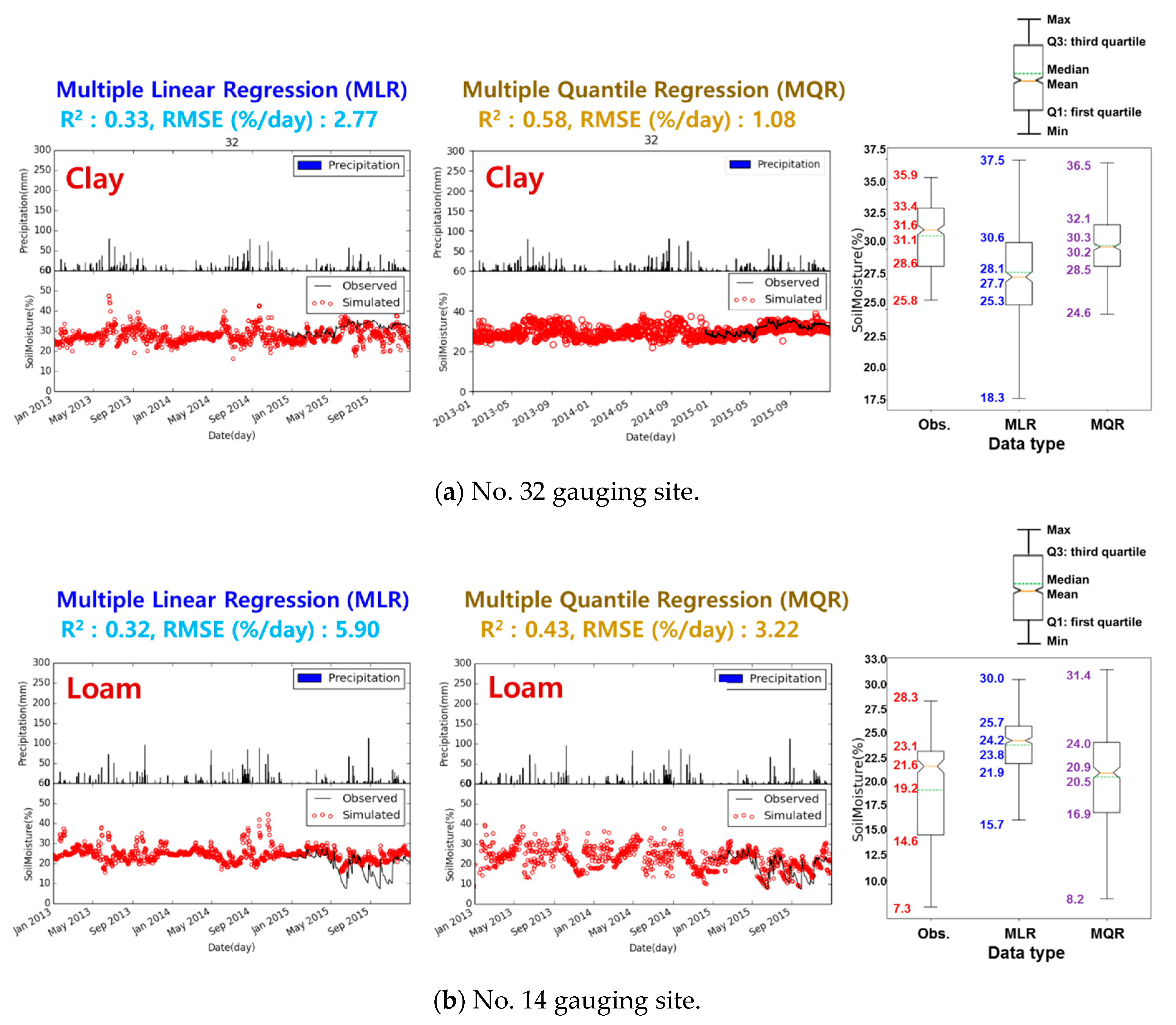
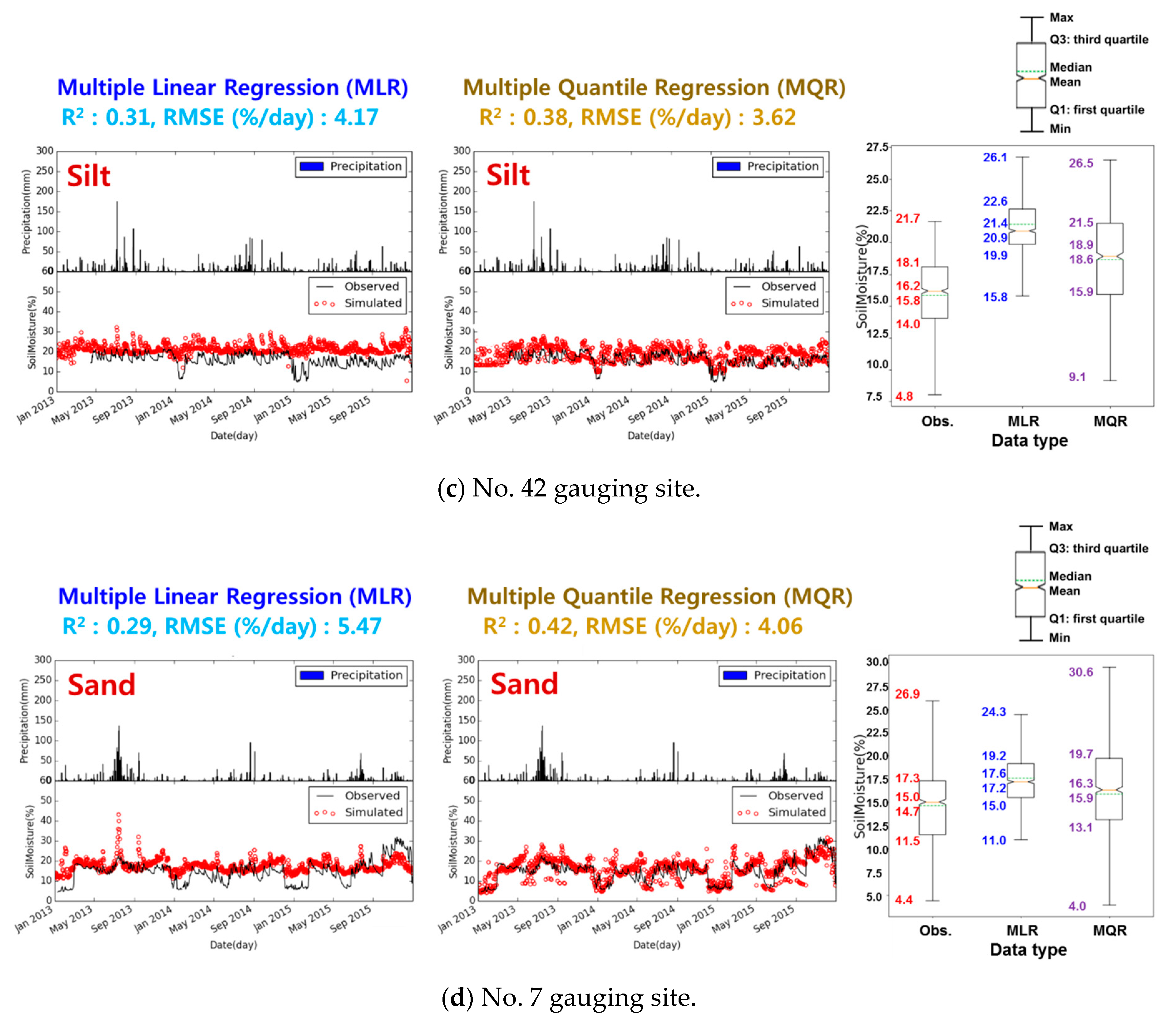
3.3. Performance Comparison between The MLR And MQR Models

Based on the estimated regression coefficients, SM was calculated for each LST quantile ranging from 10% to 90% and compared with the observed SM. The verification results were shown using R², root mean square error (RMSE) and index of agreement (IOA) to show the extent to which the results were better than those of the previous study using MLR (

Table 4. Comparison of the statistical analysis results between the multiple linear regression (MLR) and MQR models at 58 SM stations.

Station No.	R2		RMSE (%/Day)		IOA		Station No.	R2		RMSE (%/Day)		IOA
	MLR	MQR	MLR	MQR	MLR	MQR		MLR	MQR	MLR	MQR	MLR	MQR
1	0.24	0.44	4.66	4.02	0.62	0.79	30	0.34	0.77	2.55	1.98	0.38	0.49
2	0.26	0.35	9.64	6.36	0.75	0.85	31	0.45	0.60	3.74	2.70	0.72	0.74
3	0.29	0.35	12.21	7.23	0.60	0.77	32	0.33	0.58	2.77	1.08	0.61	0.64
4	0.25	0.36	5.88	4.91	0.81	0.85	33	0.53	0.57	5.91	2.78	0.69	0.72
5	0.48	0.60	5.61	3.11	0.82	0.86	34	0.37	0.57	3.42	2.41	0.45	0.58
6	0.34	0.65	3.21	2.02	0.70	0.76	35	0.31	0.33	4.04	4.01	0.63	0.64
7	0.29	0.42	5.47	4.06	0.73	0.73	36	0.51	0.65	3.55	1.36	0.62	0.70
8	0.48	0.50	3.62	3.22	0.68	0.69	37	0.40	0.58	2.55	2.43	0.72	0.74
9	0.35	0.38	3.53	3.05	0.85	0.87	38	0.40	0.57	2.76	2.34	0.21	0.49
10	0.66	0.72	3.82	3.10	0.62	0.68	39	0.25	0.57	4.31	2.43	0.60	0.74
11	0.43	0.48	3.56	3.16	0.66	0.75	40	0.35	0.52	1.86	1.53	0.43	0.61
12	0.38	0.43	3.91	3.09	0.73	0.78	41	0.33	0.57	5.22	2.55	0.17	0.54
13	0.41	0.44	3.68	3.19	0.63	0.75	42	0.31	0.38	4.17	3.62	0.30	0.62
14	0.32	0.43	4.74	3.22	0.49	0.66	43	0.45	0.63	2.48	1.77	0.58	0.63
15	0.52	0.62	3.80	2.08	0.43	0.75	44	0.39	0.59	3.65	2.38	0.45	0.72
16	0.42	0.45	3.10	3.01	0.62	0.81	45	0.40	0.57	3.24	2.52	0.41	0.61
17	0.59	0.67	2.59	2.34	0.48	0.77	46	0.32	0.36	4.09	3.82	0.88	0.81
18	0.58	0.68	3.31	2.92	0.42	0.69	47	0.34	0.61	4.46	2.05	0.53	0.64
19	0.41	0.45	3.71	3.53	0.55	0.70	48	0.40	0.47	3.75	2.67	0.82	0.82
20	0.48	0.55	3.26	2.25	0.46	0.58	49	0.32	0.38	4.91	4.05	0.41	0.66
21	0.44	0.50	3.63	3.61	0.54	0.67	50	0.31	0.62	3.86	1.75	0.51	0.67
22	0.28	0.39	5.09	4.63	0.52	0.64	51	0.30	0.33	3.11	2.89	0.55	0.59
23	0.35	0.66	3.32	2.69	0.21	0.56	52	0.20	0.25	4.42	3.60	0.27	0.37
24	0.35	0.38	4.06	3.70	0.43	0.66	53	0.26	0.36	4.80	3.65	0.47	0.58
25	0.35	0.38	4.25	3.56	0.24	0.30	54	0.32	0.64	3.12	1.75	0.18	0.57
26	0.34	0.38	3.06	3.01	0.40	0.64	55	0.41	0.61	3.39	2.21	0.49	0.64
27	0.31	0.57	4.16	2.09	0.64	0.68	56	0.41	0.60	3.46	2.56	0.75	0.77
28	0.30	0.35	4.57	3.90	0.67	0.68	57	0.20	0.30	5.22	3.57	0.33	0.59
29	0.39	0.58	4.62	1.88	0.51	0.75	58	0.35	0.38	5.55	5.23	0.60	0.64

Note: R²: coefficient of determination; RMSE: root mean square error; and IOA: index of agreement.

) [5]. The RMSE means that the error of the model is less as it approaches 0, and the IOA ranges from 0 and 1, indicating better efficiency when the value closer to 1 [46]. Figure 5 shows the time series changes in the observed SM and calculated SM through the MLR and MQR models. These representative stations in Figure 5 were recommended by a previous paper from Jung et al. [5]. From that paper, those selected were defined by considering physical characteristics, which were field capacity (FC) and wilting point (WP), to each soil type.

The SM calculated through the MLR model showed R² values from 0.2 to 0.66 for the four soil types, and the average R² was 0.37. The RMSE ranged from 1.86% to 12.21%, and the average RMSE was 4.15%. In contrast, the R² and RMSE values for the MQR results ranged from 0.25 to 0.77, with an average of 0.50, and from 1.08% to 7.23%, with an average of 3.04%, respectively. While the average IOA of SM estimated by MLR was 0.54, and ranged from 0.17 to 0.88, the average IOA by MQR was 0.68, and showed a value from 0.3 to 0.87. From these results, the MQR results showed much better performance than the MLR results. The average R², RMSE, and IOA improved by 0.13, 1.1%, and 0.14, respectively. These improvements came from removing uncertainty from measurement errors due to freezing and mechanical errors by IF and the advanced regression algorithm. However, because the soil map provided in this study consisted of four types, the SM prediction of the general MLR study caused these errors. Therefore, the MQR algorithm overcame the limitation by estimating the various regression equations under detailed conditions, such as season, soil types, and LST quantiles.

In Figure 5, the MLR results were reevaluated based on the method and information in Jung et al. [5]. Notably, each box plot shows that the MQR SM is closer to observed SM than the MLR SM. At the 32 gauging sites in clay, the first quartile (Q1) values of the observed SM, MLR SM, and MQR SM were 28.6, 25.3, and 28.4, respectively. At these stations, Q1 by MQR showed a significant improvement. The absolute percent errors for Q1 of the MLR and MQR were 34.8% and 14.2%, respectively. The MQR result was better than that of the MLR result by 20.6%. At the 14 gauging sites in loam, the Q1 values of the observed SM, MLR SM, and MQR SM were 14.6, 21.9, and 16.9, respectively. The third quartile (Q3) values of the observed SM, MLR SM, and MQR SM were 23.1, 25.7, and 24.0, respectively. At these stations, Q1 and Q3 of the MQR showed significant improvements. The Q1 absolute percent errors of MLR and MQR were 49.8% and 15.6%, respectively. The Q3 absolute percent errors of MLR and MQR were 11.1% and 3.9%, respectively. The MQR produced improvements of 34.2% for Q1 and 7.2% for Q3 over the MLR results. At the 42 gauging sites in silt, the Q1 values of the observed SM, MLR SM, and MQR SM were 14.0, 19.9, and 15.9, respectively. At these stations, Q1 of the MQR showed significant improvements. The Q1 absolute percent errors of MLR and MQR were 41.5% and 13.4%, respectively. The MQR result was 28.1% better than that of the MLR result. At the seven gauging sites in sand, the Q1 values of the observed SM, MLR SM, and MQR SM were 11.5, 15.6, and 13.1, respectively. At these stations, Q1 of the MQR showed significant improvements. The Q1 absolute percent errors of MLR and MQR were 34.8% and 14.2%, respectively. The MQR result was 20.6% better than the MLR result.

4. Discussion

4.1. Limitation of the MQR Model

Although the model was improved, there were some results that show poor accuracy. They could have been caused by the non-standardized of the algorithm and the limitation of observed data. Moreover, ignoring other variables that might impact on the estimation of soil moisture can reduce model efficiency for the prediction of soil moisture. This study did not consider elevation and slope as geophysical features; however, these variables are factors that can explain water flows under the land surface. Of these results, SW, JJ3, CC4, TG2, and HH6, which showed low performance of the model, have low elevation and slope at the same time. The elevations were 40 m (SW), 12 m (JJ3), 9 m (CC4), 11 m (TG2), and 3 m (HH6), respectively. The slopes of these stations were all about 0%, respectively.

To simply go over in terms of these effects, SM variation by PCP as natural inflow for these five stations was analyzed. As seen in

Table 5. The additional features to review limitation of this MQR result: elevation, slope, and seasonal SM.

No.	Station	Elevation (m)	Slope (%)	Soil Moisture (%/Day)
				Year	PCP over 5 mm/d	PCP less than 5 mm/d
2	SW	40	0.40	2013	13.6	17.3
				2014	12.0	14.1
				2015	12.1	14.9
				Mean	12.5	15.6
28	JJ3	12	0.12	2013	19.3	19.9
				2014	18.7	19.4
				2015	23.1	23.3
				Mean	20.6	20.9
49	CC4	9	0.09	2013	22.3	25.7
				2014	21.5	23.3
				2015	19.7	20.5
				Mean	20.9	23.0
53	TG2	11	0.11	2013	18.7	23.4
				2014	21.7	22.5
				2015	20.9	22.5
				Mean	20.7	22.7
58	HH6	3	0.03	2013	22.3	24.6
				2014	21.9	21.7
				2015	25.5	24.9
				Mean	23.4	23.6

Note: PCP over 5 mm/d (SM when PCP is over 5 mm/day); PCP less than 5 mm/d (SM when PCP is less than 5 mm/day).

, these results show that average daily SM, when PCP was less than 5 mm/day (dry SM), was slightly bigger than SM when PCP was over 5 mm/day (wet SM), which means that this trend was unlike normal SM tendency. Moreover, dry SM at the SW station increased an average 3.1% compared to wet SM. The reason for this tendency is that these five stations are in the area around the river or relatively close to the river than the other 53 stations. In this area, the interaction between surface water and groundwater occurs actively. Thus, it would cause a strong dynamic movement of soil moisture. This result is a fragmentary analysis, which is difficult to generalize, but it is necessary to consider those variables as a further review.

4.2. Extension of Input Variables

In some papers for estimating SM, various factors applied such as albedo, brightness, greenness, wetness, NDVI, normalized difference water index (NDWI), normalized difference built-up index (NDBI), elevation, slope, and aspect [30]. It is thought that adding these variables will improve SM prediction performance, but it has not been applied in this study. This is because the purpose of this study was to evaluate how much performance could be improved by the MQR model compared to that of the MLR model in the previous study [5], after filtering SM outliers. In addition, it could be expected to improve the simulation performance by applying the temperature vegetation dryness index (TVDI) [25], considering vegetation (NDVI) and land surface temperature (LST).

Even though this study did not consider the additional variables, we proceeded to improve the existing simple algorithm based on the satellite image LST data. This study achieved meaningful results; however, it is still necessary to consider the areas that did not improve significantly. Although the accuracy of the model could be improved by adding new variables, as the variables become more complex, multicollinearity between variables and overfitting of untrained variables would increase. This can lead to significant side effects for the non-verified period.

Nevertheless, as mentioned in Section 4.1, considering the hydrological system of soil moisture, we found out that the elevation, slope, and distance from the stream will have an additional effect. Based on surface and groundwater flows, it could be determined that the elevation and slope values would increase the movement of moisture due to slope in the soil. Furthermore, the soil moisture in the area close to the river may be sensitive to the influence of groundwater in addition to precipitation and soil characteristics. Therefore, if sufficient data are available, it is expected that future studies will greatly improve this algorithm.

5. Conclusions

This study aimed to improve the original MLR algorithm for the indirect measurement of spatial SM. To improve the original algorithm, this study first performed outlier detection of observed SM using the IF method, which is a type of machine learning, and the spatial distribution of SM was estimated using an MQR model from 2013 to 2015. As input for the MQR algorithm, MODIS LST, MODIS NDVI, precipitation, and the soil type were used as independent variables, with consideration for the environmental attributes of SM. Because of the limitation of insufficient data, the soil type was reclassified into four soil classes: silt, clay, loam, and sand. For this reason, the soil information at 58 stations was not uniformly distributed, and certain soils were more common. Therefore, this study had to classify four soil types. The primary results are summarized as follows:

• As a result of outlier detection, the average DRRs for IF1 and IF2 were 23.6% and 14.4%, respectively, at 58 stations. In addition, average COR_PCP for IF1 and IF2 were 29.9% and 37.6%, respectively. The result of IF2 shows that the IF algorithm considering PCP (precipitation) can improve suitability of the outlier detection. Finally, the IF2 result was used as an input variable.
• When comparing the MLR and MQR results, the R² and RMSE values for MLR were 0.20 to 0.66 and 1.86% to 12.21%/day, respectively, while the R² and RMSE values for MQR were 0.25 to 0.77 and 1.08% and 7.23%/day, respectively. From these results, the R² improved by 0.13 from an average of 0.38 to 0.50, and the RMSE decreased by 1.1%/day errors from an average of 4.15% to 3.05%/day.
• Finally, in addition to improvement in accuracy, box plots were constructed for the four major stations representing each of the soil types to match the cumulative distribution functions (CDF) between observed SM and estimated SM, including MLR and MQR. At these stations, Q1 and Q3 of the MQR showed significant improvements. The Q1 and Q3 absolute percent errors for the MQR improved by 25.9% and 5.2%, respectively.

The method of the indirect measurement of spatial SM using MODIS LST, NDVI, and antecedent precipitation from the previous study [5] was verified. Additionally, MODIS LST corrected by the CM technique ensured the reliability of the data. Compared to previous results from the MLR model, improvements were seen not only in the R² of the MQR model, showing a 62% (0.37 to 0.50) improvement, but also in the distribution of the MQR, such that the CDF was close to the distribution of observed SM. This method overcame the limitations of the previous model by improving both the bias and variance. Nevertheless, since there were not enough data spanning more than two years at most stations, all data spanning less than two years were used to train the MQR model. Therefore, this study could have an overfitting problem for prediction. Future research could resolve this issue by obtaining more than two years’ worth of observed SM data and by splitting the acquired data into training and verification subsets.

References

1. Seneviratne, S.I.; Corti, T.; Davin, E.L.; Hirschi, M.; Jaeger, E.B.; Lehner, I.; Orlowsky, B.; Teuling, A.J. Investigating soil moisture–climate interactions in a changing climate: A review. Earth Sci. Rev. 2010, 99, 125–161. [Google Scholar] [CrossRef]
2. Gevaert, A.I.; Parinussa, R.M.; Renzullo, L.J.; van Dijk, A.I.J.M.; de Jeu, R.A.M. Spatio-temporal evaluation of resolution enhancement for passive microwave soil moisture and vegetation optical depth. Int. J. Appl. Earth Obs. Geoinf. 2016, 45, 235–244. [Google Scholar] [CrossRef]
3. Torres-Rua, F.A.; Ticlavilca, M.A.; Bachour, R.; McKee, M. Estimation of surface soil moisture in irrigated lands by assimilation of landsat vegetation indices, surface energy balance products, and relevance vector machines. Water 2016, 8, 167. [Google Scholar] [CrossRef] [Green Version]
4. Carlson, T.; Gillies, R.; Perry, E. A method to make use of thermal infrared temperature and NDVI measurements to infer surface soil water content and fractional vegetation cover. Remote Sens. Rev. 1994, 9, 161–173. [Google Scholar] [CrossRef]
5. Jung, C.G.; Lee, Y.G.; Cho, Y.; Kim, S. A study of spatial soil moisture estimation using a multiple linear regression model and MODIS land surface temperature data corrected by conditional merging. Remote Sens. 2017, 9, 870. [Google Scholar] [CrossRef] [Green Version]
6. Njoku, E.; Wilson, W.; Yueh, S.; Dinardo, S.; Li, F.; Jackson, T.; Lakshmi, V.; Bolten, J. Observations of soil moisture using a passive and active low-frequency microwave airborne sensor during SGP99. IEEE Trans. Geosci. Remote Sens. 2003, 40, 2659–2673. [Google Scholar] [CrossRef]
7. Ulaby, F.T.; Dubois, P.C.; van Zyl, J. Radar mapping of surface soil moisture. J. Hydrol. 1996, 184, 57–84. [Google Scholar] [CrossRef]
8. Fang, B.; Lakshmi, V.; Jackson, T.J.; Bindlish, R.; Colliander, A. Passive/active microwave soil moisture change disaggregation using SMAPVEX12 data. J. Hydrol. 2019, 574, 1085–1098. [Google Scholar] [CrossRef]
9. White, J.; Berg, A.A.; Champagne, C.; Warland, J.; Zhang, Y. Canola yield sensitivity to climate indicators and passive microwave-derived soil moisture estimates in Saskatchewan, Canada. Agric. For. Meteorol. 2019, 268, 354–362. [Google Scholar] [CrossRef]
10. Dong, J.; Crow, W.T.; Tobin, K.J.; Cosh, M.H.; Bosch, D.D.; Starks, P.J.; Seyfried, M.; Collins, C.H. Comparison of microwave remote sensing and land surface modeling for surface soil moisture climatology estimation. Remote Sens. Environ. 2020, 242, 111756. [Google Scholar] [CrossRef]
11. Ye, N.; Walker, J.P.; Rüdiger, C.; Ryu, D.; Gurney, R.J. Surface rock effects on soil moisture retrieval from L-band passive microwave observations. Remote Sens. Environ. 2018, 215, 33–43. [Google Scholar] [CrossRef]
12. Su, C.-H.; Ryu, D.; Western, A.W.; Wagner, W. De-noising of passive and active microwave satellite soil moisture time series. Geophys. Res. Lett. 2013, 40, 3624–3630. [Google Scholar] [CrossRef]
13. Lei, F.; Crow, W.T.; Shen, H.; Su, C.-H.; Holmes, T.R.H.; Parinussa, R.M.; Wang, G. Assessment of the impact of spatial heterogeneity on microwave satellite soil moisture periodic error. Remote Sens. Environ. 2018, 205, 85–99. [Google Scholar] [CrossRef]
14. Bartalis, Z.; Wagner, W.; Naeimi, V.; Hasenauer, S.; Scipal, K.; Bonekamp, H.; Figa, J.; Anderson, C. Initial soil moisture retrievals from the METOP-A Advanced Scatterometer (ASCAT). Geophys. Res. Lett. 2007, 34, L20401. [Google Scholar] [CrossRef] [Green Version]
15. Kerr, Y.; Philippe, W.; Richaume, P.; Wigneron, J.-P.; Ferrazzoli, P.; Mahmoodi, A.; Al Bitar, A.; Cabot, F.; Gruhier, C.; Juglea, S.; et al. The SMOS soil moisture retrieval algorithm. IEEE Trans. Geosci. Remote Sens. 2012, 50, 1384–1403. [Google Scholar] [CrossRef]
16. Njoku, E.; Jackson, T.; Lakshmi, V.; Chan, T.; Nghiem, S. Soil moisture retrieval from AMSR-E. IEEE Trans. Geosci. Remote Sens. 2003, 41, 215–229. [Google Scholar] [CrossRef]
17. De Jeu, R.A.M.; Wagner, W.; Holmes, T.R.H.; Dolman, A.J.; van de Giesen, N.C.; Friesen, J. Global soil moisture patterns observed by space borne microwave radiometers and scatterometers. Surv. Geophys. 2008, 29, 399–420. [Google Scholar] [CrossRef] [Green Version]
18. Owe, M.; de Jeu, R.; Holmes, T. Multisensor historical climatology of satellite-derived global land surface moisture. J. Geophys. Res. 2008, 113, F01002. [Google Scholar] [CrossRef]
19. Werbylo, K.L.; Niemann, J.D. Evaluation of sampling techniques to characterize topographically-dependent variability for soil moisture downscaling. J. Hydrol. 2014, 516, 304–316. [Google Scholar] [CrossRef] [Green Version]
20. Djamai, N.; Magagi, R.; Goïta, K.; Merlin, O.; Kerr, Y.; Roy, A. A combination of DISPATCH downscaling algorithm with CLASS land surface scheme for soil moisture estimation at fine scale during cloudy days. Remote Sens. Environ. 2016, 184, 1–14. [Google Scholar] [CrossRef]
21. Kang, J.; Jin, R.; Li, X.; Ma, C.; Qin, J.; Zhang, Y. High spatio-temporal resolution mapping of soil moisture by integrating wireless sensor network observations and MODIS apparent thermal inertia in the Babao River Basin, China. Remote Sens. Environ. 2017, 191, 232–245. [Google Scholar] [CrossRef] [Green Version]
22. Lee, Y.; Jung, C.; Kim, S. Spatial distribution of soil moisture estimates using a multiple linear regression model and Korean geostationary satellite (COMS) data. Agric. Water Manag. 2019, 213, 580–593. [Google Scholar] [CrossRef]
23. Holzman, M.E.; Rivas, R.; Piccolo, M.C. Estimating soil moisture and the relationship with crop yield using surface temperature and vegetation index. Int. J. Appl. Earth Obs. Geoinf. 2014, 28, 181–192. [Google Scholar] [CrossRef]
24. Mallick, K.; Bhattacharya, B.K.; Patel, N.K. Estimating volumetric surface moisture content for cropped soils using a soil wetness index based on surface temperature and NDVI. Agric. For. Meteorol. 2009, 149, 1327–1342. [Google Scholar] [CrossRef]
25. Sandholt, I.; Rasmussen, K.; Andersen, J. A simple interpretation of the surface temperature/vegetation index space for assessment of surface moisture status. Remote Sens. Environ. 2002, 79, 213–224. [Google Scholar] [CrossRef]
26. Jackson, R.D.; Reginato, R.J.; Idso, S.B. Wheat canopy temperature: A practical tool for evaluating water requirements. Water Resour. Res. 1977, 13, 651–656. [Google Scholar] [CrossRef]
27. Jackson, R.D.; Idso, S.B.; Reginato, R.J.; Pinter, P.J., Jr. Canopy temperature as a crop water stress indicator. Water Resour. Res. 1981, 17, 1133–1138. [Google Scholar] [CrossRef]
28. Jackson, R.D. Canopy temperature and crop water stress. In Advances in Irrigation; Hillel, D., Ed.; Academic Press: New York, NY, USA, 1982; pp. 43–85. [Google Scholar]
29. Gillies, R.R.; Kustas, W.P.; Humes, K.S. A verification of the ‘triangle’ method for obtaining surface soil water content and energy fluxes from remote measurements of the normalized difference vegetation index (NDVI) and surface e. Int. J. Remote Sens. 1997, 18, 3145–3166. [Google Scholar] [CrossRef]
30. Fathololoumi, S.; Vaezi, A.R.; Alavipanah, S.K.; Ghorbani, A.; Biswas, A. Comparison of spectral and spatial-based approaches for mapping the local variation of soil moisture in a semi-arid mountainous area. Sci. Total Environ. 2020, 724, 138319. [Google Scholar] [CrossRef]
31. Mohseni, F.; Mokhtarzade, M. A new soil moisture index driven from an adapted long-term temperature-vegetation scatter plot using MODIS data. J. Hydrol. 2020, 581, 124420. [Google Scholar] [CrossRef]
32. Long, D.; Bai, L.; Yan, L.; Zhang, C.; Yang, W.; Lei, H.; Quan, J.; Meng, X.; Shi, C. Generation of spatially complete and daily continuous surface soil moisture of high spatial resolution. Remote Sens. Environ. 2019, 233, 111364. [Google Scholar] [CrossRef]
33. Hassan, A.M.; Belal, A.A.; Hassan, M.A.; Farag, F.M.; Mohamed, E.S. Potential of thermal remote sensing techniques in monitoring waterlogged area based on surface soil moisture retrieval. J. Afr. Earth Sci. 2019, 155, 64–74. [Google Scholar] [CrossRef]
34. Fang, B.; Lakshmi, V.; Bindlish, R.; Jackson, T.J.; Liu, P. Evaluation and Validation of a High Spatial Resolution Satellite Soil Moisture Product over the Continental United States. J. Hydrol. 2020, 125043. [Google Scholar] [CrossRef]
35. Lee, Y.G.; Kim, S. The modified SEBAL for mapping daily spatial evapotranspiration of South Korea using three flux towers and Terra MODIS data. Remote Sens. 2016, 8, 983. [Google Scholar] [CrossRef] [Green Version]
36. Ozelkan, E.; Bagis, S.; Ozelkan, E.C.; Ustundag, B.B.; Yucel, M.; Ormeci, C. Spatial interpolation of climatic variables using land surface temperature and modified inverse distance weighting. Int. J. Remote Sens. 2015, 36, 1000–1025. [Google Scholar] [CrossRef]
37. Or, D.; Hanks, R.J. Spatial and temporal soil water estimation considering soil variability and evapotranspiration uncertainty. Water Resour. Res. 1992, 28, 803–814. [Google Scholar] [CrossRef]
38. Mohanty, B.P.; Skaggs, T.H.; Famiglietti, J.S. Analysis and mapping of field-scale soil moisture variability using high-resolution, ground-based data during the Southern Great Plains 1997 (SGP97) Hydrology Experiment. Water Resour. Res. 2000, 36, 1023–1031. [Google Scholar] [CrossRef] [Green Version]
39. Goudenhoofdt, E.; Delobbe, L. Evaluation of radar-gauge merging methods for quantitative precipitation estimates. Hydrol. Earth Syst. Sci. 2009, 13, 195–203. [Google Scholar] [CrossRef] [Green Version]
40. Shepard, D. A two-dimensional interpolation function for irregularly-spaced data. In Proceedings of the 1968 23rd ACM National Conference, Las Vegas, NV, USA, 27–29 August 1968; pp. 517–524. [Google Scholar] [CrossRef]
41. Ding, Z.; Fei, M. An anomaly detection approach based on isolation forest algorithm for streaming data using sliding window. IFAC Proc. Vol. 2013, 46, 12–17. [Google Scholar] [CrossRef]
42. Chen, W.; Yun, Y.-H.; wen, M.; Lu, H.; Zhang, Z.; Liang, Y. Representative subset selection and outlier detection via isolation forest. Anal. Methods 2016, 8, 7225–7231. [Google Scholar] [CrossRef]
43. Koenker, R.; Bassett, G. Regression quantiles. Econometrica 1978, 46, 33–50. [Google Scholar] [CrossRef]
44. Melly, B. Decomposition of differences in distribution using quantile regression. Labour Econ. 2005, 12, 577–590. [Google Scholar] [CrossRef] [Green Version]
45. Koenker, R.; Hallock, K.F. Quantile regression. J. Econ. Perspect. 2001, 15, 143–156. [Google Scholar] [CrossRef]
46. Moriasi, D.N.; Arnold, J.G.; Van Liew, M.W.; Bingner, R.L.; Harmel, R.D.; Veith, T.L. Model evaluation guidelines for systematic quantification of accuracy in watershed simulations. Trans. ASABE 2007, 50, 885–900. [Google Scholar] [CrossRef]
Figure 1. The study procedures.
Remotesensing 12 01678 g001
Figure 2. Observation stations: (a) the 687 automatic weather stations (AWS) and (b) the 58 soil moisture stations run by various institutions with elevation.
Remotesensing 12 01678 g002
Figure 3. Overview of the isolation forest method. Light green circles represent common normal samples, dark green circles represent uncommon normal samples, and red circles represent outliers.
Remotesensing 12 01678 g003
Figure 4. The graphs between original observed soil moisture (raw data) and observed soil moisture (SM) removed by isolation forest (IF) considering precipitation (PCP). Blue circles represent the original observed soil moisture before applying the IF method, and red Xs represent observed soil moisture after applying the IF method.
Remotesensing 12 01678 g004
Figure 5. Comparison graphs of observed SM and estimated SM for each soil type between multiple linear regression (MLR) and quantile regression (MQR). Additionally, the box plots are illustrated.
Remotesensing 12 01678 g005aRemotesensing 12 01678 g005b