Mapping the Global Mangrove Forest Aboveground Biomass Using Multisource Remote Sensing Data


1
State Key Laboratory of Vegetation and Environmental Change, Institute of Botany, Chinese Academy of Sciences, Beijing 100093, China
2
University of Chinese Academy of Sciences, Beijing 100049, China
3
Department of Earth System Science, Tsinghua University, Beijing 100084, China
*
Author to whom correspondence should be addressed.
Remote Sens. 2020, 12(10), 1690; https://0-doi-org.brum.beds.ac.uk/10.3390/rs12101690
Submission received: 28 April 2020
/
Revised: 19 May 2020
/
Accepted: 20 May 2020
/
Published: 25 May 2020
(This article belongs to the Special Issue Remote Sensing in Mangroves)
Abstract
:Mangrove forest ecosystems are distributed at the land–sea interface in tropical and subtropical regions and play an important role in carbon cycles and biodiversity. Accurately mapping global mangrove aboveground biomass (AGB) will help us understand how mangrove ecosystems are affected by the impacts of climatic change and human activities. Light detection and ranging (LiDAR) techniques have been proven to accurately capture the three-dimensional structure of mangroves and LiDAR can estimate forest AGB with high accuracy. In this study, we produced a global mangrove forest AGB map for 2004 at a 250-m resolution by combining ground inventory data, spaceborne LiDAR, optical imagery, climate surfaces, and topographic data with random forest, a machine learning method. From the published literature and free-access datasets of mangrove biomass, we selected 342 surface observations to train and validate the mangrove AGB estimation model. Our global mangrove AGB map showed that average global mangrove AGB density was 115.23 Mg/ha, with a standard deviation of 48.89 Mg/ha. Total global AGB storage within mangrove forests was 1.52 Pg. Cross-validation with observed data demonstrated that our mangrove AGB estimates were reliable. The adjusted coefficient of determination (R2) and root-mean-square error (RMSE) were 0.48 and 75.85 Mg/ha, respectively. Our estimated global mangrove AGB storage was similar to that predicted by previous remote sensing methods, and remote sensing approaches can overcome overestimates from climate-based models. This new biomass map provides information that can help us understand the global mangrove distribution, while also serving as a baseline to monitor trends in global mangrove biomass.
1. Introduction
Mangrove forests are important intertidal ecosystems that link terrestrial and marine systems [1], protecting land from the impact of storm surges, waves, and the erosion of the shore [2,3,4]. Mangrove plays a major role in the carbon cycle and helps maintain biodiversity. These forests cover only 2% of the world’s coastal areas, yet they provide 5% of the net primary production of global coastal ecosystems [5,6]. While mangrove forests comprise only 0.7% of the area of tropical forests [7], their total carbon density is four times that of other tropical forests in the Indo-Pacific region [8]. Mangrove forests consist of approximately seventy taxonomically diverse tree, shrub, and fern species [9,10,11]. Moreover, mangrove is an important habit for other organisms [12], such as birds [13] and fish [14], such as mangroves in the Caribbean that have strong effect on the community structure of fish living in the coral reef [14].
Currently, mangroves are highly threatened by both climate change and human activities. As a result of global warming, suitable habitats for mangrove in tropical and subtropical areas have expanded poleward, but sea level rise may be a major threat to the mangrove forests as a result of changes in swamp duration, frequency, or salinity [15,16]. During the past century, approximately 35% of the area with mangrove forests has disappeared [17]. There is an annual deforestation rate of 1–3% [1,17,18,19,20] as these areas are converted for use in aquaculture or agriculture [21]. The amount of and change in aboveground biomass act as indicators of other ecosystem services, such as biodiversity [22]. For example, studies indicate a degraded mangrove forest in Malaysia can lose half of its aboveground biomass (AGB) when compared to a natural mangrove forest [22]. Consequently, accurate estimates of the global distribution of mangrove aboveground biomass is beneficial for our understanding of the status of mangrove ecosystems under threat from deforestation and degradation.
Field surveys are the most basic and most accurate methods for acquiring mangrove AGB at the local scale [23,24,25,26,27,28]. However, this method is time-consuming and costly when applied to larger areas while providing only discrete measurements of AGB at specified points [29,30]. Moreover, field surveys in mangrove areas are more difficult than surveys in other terrestrial ecosystems due to the muddy conditions and the peculiar structure of mangroves [9]. There are two additional methods for estimating regional or global mangrove AGB: model-based methods and remote sensing. Model-based methods usually provide mangrove AGB estimations from local to global scales based on a relationship between environmental drivers and mangrove biomass [31,32,33]. However, model-based methods usually reflect potential biomass distribution, which is often inconsistent with actual distribution. Remote sensing methods provide an indirect approach for obtaining mangrove AGB measurements using regression models built by linking surface measurements with remote sensing data. Development of these remote sensing methods has greatly improved the efficiency and lowered the cost of mapping mangrove AGB at large scales [34,35].
There are three popular remote sensing techniques for estimating mangrove biomass: passive optical remote sensing, radar, and light detection and ranging (LiDAR) [36]. Passive optical remote sensing and radar are the earliest and most frequently used methods for estimating mangrove extent and biomass mapping [35,37,38], since they have the benefit of complete global coverage and the data are easily accessible. However, both passive optical remote sensing and radar suffer from a saturation effect at high biomass levels. Neither of these methods can retrieve complete vertical canopy information because optical remote sensing only acquires canopy surface information and radar has limited penetration ability [39].
An active remote sensing method, light detection and ranging, effectively penetrates the forest canopy and can be used to derive information about forest structure in three dimensions [40,41]. Because of its ability to quantify forest height, AGB, and other structural parameters in a variety of forest environments, LiDAR is a major advance in the field of forestry remote sensing [42,43]. Moreover, LiDAR does not saturate at high biomass [44,45]. Current limitations in temporal and spatial coverage restrict the application of LiDAR at continental to global scales [46,47]. Airborne and spaceborne LiDAR can acquire large scale data, but neither can provide worldwide, continuous LiDAR measurements. The high cost of flight missions limits the use of airborne LiDAR to certain regions. Spaceborne LiDAR such as the Geoscience Laser Altimeter System (GLAS) onboard the Ice, Cloud, and Land Elevation Satellite (ICESat) have collected global LiDAR measurements, but the low density and discontinuous distribution of the GLAS footprint prevents direct production of continuous global data [48,49].
Recently, studies have demonstrated that using multi-source data can overcome the deficiencies associated with GLAS data [48,49]. Passive optical images along with other continuous variables, such as climate layers and a digital terrain model, can be used to build a regression model with GLAS measurements, allowing us to extrapolate from discrete GLAS pixels into spatially continuous layers [46,47]. This method has been used to estimate forest biomass at the scale of the GLAS footprint through a direct-link method proposed by Baccini et al. [50]. A second method uses airborne LiDAR as a medium [51], thereby extrapolating from discrete AGB points into full coverage layers. However, airborne LiDAR and plots in areas of mangrove are limited, and it is not possible to combine field measurements with GLAS data. Another method suggested by Su et al. [47] provides wall-to-wall estimates of forest AGB at larger scales. First, continuous remote sensing data are used to extrapolate discrete GLAS parameters into spatially continuous layers. Second, a model is built using surface observations rather than linking plot data directly with GLAS data.
Although global mangrove biomass estimates have been generated in the past using climate-based [31,32] and remote sensing [52,53] methods, these results have had little explanatory power or suffer from signal saturation. Moreover, structural information obtained using LiDAR were not fully utilized in previous efforts to map global mangrove biomass. The objectives of this study, then, were to estimate global mangrove AGB using ground inventory data, spaceborne LiDAR, and other multi-source data and then to determine if structural information provided by GLAS can improve our understanding of the distribution of mangrove AGB. To meet these objectives, a map of global mangrove AGB map at 250 m has been created and will be disseminated via the internet. This new biomass map provides information about mangrove forests, allowing us to better monitor regional and global biomass trends into the future.
2. Materials and Methods
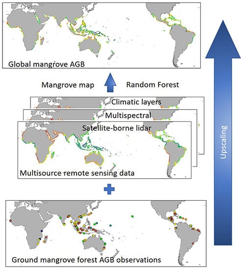
The global map of mangrove AGB was generated using field observation data, GLAS data, the enhanced vegetation index (EVI), topographic data, and climate data. The methodology outlined in Figure 1 allowed us to successfully estimate nation-wide forest AGB for China [47] and global forest AGB [46]. A detailed description of each dataset (Table 1) and a brief introduction to the method used to estimate mangrove forest AGB are provided below.
2.1. Surface Measurements of Mangrove AGB
Field data are fundamental for estimating mangrove AGB from remote sensing data. In this study, we obtained 510 plot measurements from previously published articles and free-access mangrove biomass databases, such the Sustainable Wetlands Adaptation and Mitigation Program (https://data.cifor.org/dataverse/swamp) [57,58]. Since these in situ plot measurements were collected from a variety of sources using different protocols, we used three filtering criteria to ensure their quality: (1) the plot has a georeferenced location, (2) the inventory was taken after 2000, and (3) the site was not surveyed using harvesting methods. The geolocation of each individual plot was vital to this study. Using Google Earth, we manually checked each point to determine whether the plot location was in the ocean or on land. Records with the same geolocations were averaged together. In the end, 342 plot samples were retained for use in the mangrove AGB mapping procedures (Figure 2).
2.2. Spacebrone LiDAR Data
The GLAS instrument is the only waveform LiDAR instrument that has provided global coverage, and it was as an important data source for mapping global tree height and forest biomass. The GLAS instrument aboard the NASA (National Aeronautics and Space Administration) ICESat satellite was launched on 12 January 2003. After seven years in orbit and 18 laser-operation campaigns, the ICESat mission ended with the failure of the GLAS instrument. This instrument had three laser sensors, L1–L3, and each sensor used a 1064-nm laser pulse to record surface altimetry at 20 Hz. Each laser pulse had an ~65 m ellipsoidal footprint and was spaced at 170 m along a track with tens of kilometers between tracks [59]. We selected GLAS data from 2004 for use in mapping mangrove AGB since the quantity and quality of these GLAS data are better than those from later operational periods [46,47]. We downloaded three products (GLA01, GLA06, and GLA14) from the National Snow & Ice Data Center (https://nsidc.org/data). These three products were provided in HDF5 (Hierarchical Data Format) and contained full-waveform information (GLA01); geolocation and data quality information (GLA06); and surface elevation information (GLA14). Laser pulses from these products were linked together based on their unique ID and shot time.
Based on previous research [46,47,48,49], we applied four filtering criteria to quality control the GLAS data: (1) laser shots taken under cloudy conditions were removed; (2) data with saturation effects were removed; (3) the data had high signal to noise ratios (>50); and (4) data was not taken from a location significantly higher (i.e., >100 m) than the land surface elevation as indicated by the Shuttle Radar Topography Mission (SRTM) data. All GLAS data points used in this study were determined to be within Spalding et al.’s mangrove map [19]. The final GLAS dataset contained 13,686 records in areas of mangrove forests. From this dataset, three parameters were derived from the full-waveform information of each pulse (waveform extent, leading edge extent, and trailing edge extent). These GLAS parameters have been proven to be highly correlated with forest biomass, canopy height, canopy height variability, and slope of the terrain [48,60].
2.3. EVI Data
We used the MOD13Q1 Version 6 product to obtain cumulative EVI for 2004. The EVI has improved sensitivity for regions of high biomass as compared with NDVI [56]. MOD13Q1 is a composite 16-day product at a 250-m resolution. The composite algorithm chooses the best available pixel value from all acquisitions within the 16-day period, selecting pixels with low clouds, a low view angle, and the highest EVI value. Cumulative EVI can provide more accurate estimates of AGB when compared with values taken from a single time period [61,62]. Therefore, we calculated cumulative EVI from the sum of all collected MOD13Q1 data, and clipped it using a 100-km coastline buffer. These data were used as a predictor in the AGB analysis and mapping procedure.
2.4. Climate Data
In addition to using structure and spectral information from remote sensing data, we included climate data to use in model predictions of mangrove AGB (Table 1). We selected the WorldClim dataset (http://www.worldclim.org), and 50-year (1950–2000) average bioclimatic variables were calculated from monthly temperature and precipitation layers [54]. We selected eight climate variables that can be divided into two categories: precipitation and temperature (Table 1). The climate layers were obtained with a 1-km resolution and then downscaled to 250 m using a bilinear method.
2.5. Topography Data
The GLAS parameters are related to forest structure and terrain variation, so we used topography data to extrapolate from discrete GLAS data into spatial continuous layers. We selected the CSRTM digital elevation model (DEM) provided by Zhao et al. [55]. The CSRTM is a corrected product from the Shuttle Radar Topography Mission (SRTM), which reduced the vertical errors of SRTM at vegetated areas. To be consistent with other datasets, we resampled the CSRTM DEM into 250-m resolution using a bilinear method for further interpolation. The slope (denoted by tangent values of slope) was calculated from the resampled CSRTM DEM.
2.6. Mangrove AGB Estimation Methods
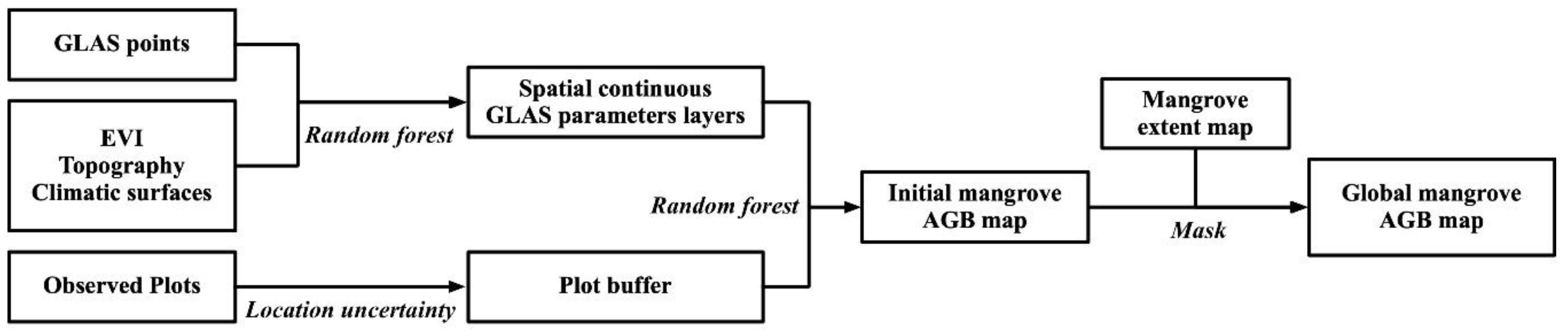
As mentioned, we estimated global mangrove AGB using a methodology that had been successfully implemented to estimate forest AGB at both national and global scales [46,47]. We modified the step regarding plot location uncertainty to account specifically for the distribution of mangrove. We did not use a land cover map in the random forest regression analysis as we assumed all areas were mangrove based on our data collection methods previous described. As shown in Figure 1, the estimation of mangrove AGB is generally divided into four major steps.
First, discrete GLAS points were interpolated to create continuous spatial layers using the random forest algorithm. The GLAS points were filtered using a 100-km coastline buffer and aggregated into 250-m pixels using the average value of the GLAS full waveform parameter within each pixel. These pixels were then used as training data to build the random forest model created to extrapolate the GLAS parameters along with other predictor layers (cumulative EVI, DEM, slope, climate surfaces) using the randomForest R package [63].
Second, we generated a circular buffer for each plot measurements with a 500-m radius to reduce uncertainty related to plot location. Since mangrove has a much smaller distribution than other forest types, we could not use the point-radius method suggested by Su et al. to reduce geolocation uncertainty [47]. Using their Monte-Carlo simulation method, generating plot sets with location errors of 1 or 10 km would relocate many mangrove plots into the ocean. To avoid this issue, we used the circular buffer method. Most latitudes and longitudes in our field observation data were accurate to 0.01°, corresponding to ~1km. We, therefore, adopted a 500-m radius to reduce location uncertainty.
Third, an initial global mangrove AGB map was created using the random forest method. Pixels for each explanatory layer within a plot buffer were averaged and used as explanatory variables to build a regression model from plot measurements. We randomly chose 70% of the plots (239 plots) to train the model and used the remaining 30% (103 plots) to validate the mangrove AGB estimation model. The three extrapolated GLAS parameters and the other nine parameters in Table 1 were used in the regression model to generate the outputs needed to produce this initial mangrove AGB map.
Finally, we used a mangrove extent map from Spalding et al. as a mask for our initial mangrove AGB map, eliminating areas outside of identified mangrove forests. [19]. The final global mangrove AGB map was obtained by setting AGB value in areas outside the mangrove extent to 0 Mg/ha.
2.7. Accuracy Assessment
The accuracy of the estimated AGB was assessed using the adjusted coefficient of determination (R2) and root-mean-square error (RMSE). The R2 and RMSE were calculated using following equations:
where is the observed mangrove AGB, is the predicted AGB based on the random forest model built with the training data, is the average AGB of all validation plots, and is the number of validation plots.
3. Results
3.1. The GLAS Parameters in the Mangrove Distribution Zone
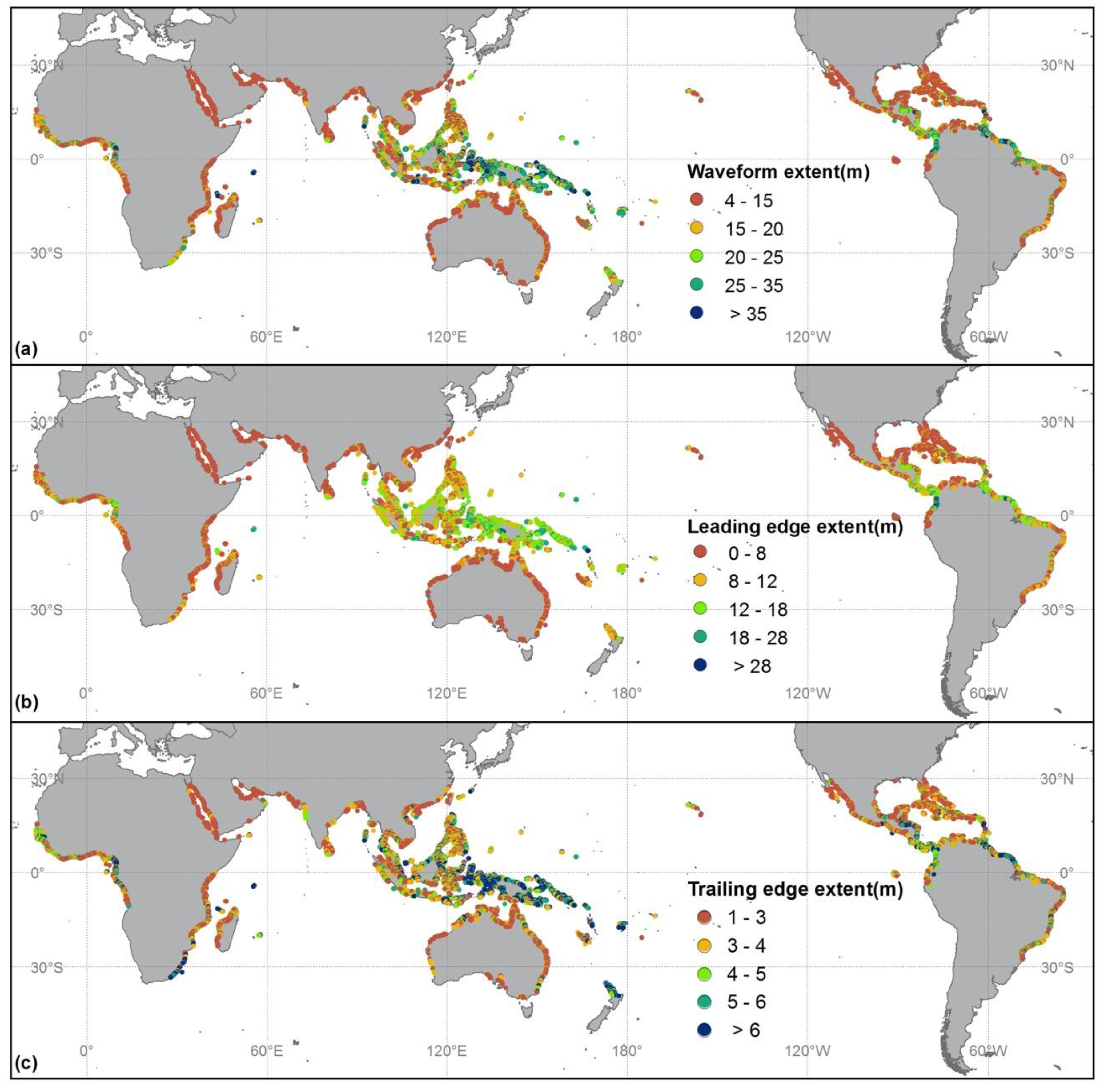
The discrete GLAS parameter points were extrapolated to spatially continuous layers using the random forest method for leading edge extent, waveform extent, and trailing edge extent (Figure 3). Overall, the random forest models explained 40.32%, 59.12%, and 41.39% of the variance in leading edge extent, waveform extent and trailing edge extent, respectively. The root-mean-square residuals for leading edge extent, waveform extent, and trailing edge extent were 4.30, 6.98, and 2.35 m, respectively. According to the extrapolated results, the mean value of leading edge extent, waveform extent, and trailing edge extent for the mangroves were 11.34 ± 5.61 m, 19.06 ± 7.09 m, 4.19 ± 1.34 m, respectively. These three GLAS parameters showed similar spatial patterns of mangrove distribution. The highest values of all three parameters appeared in the Indonesian archipelago, Central America, and the Gulf of Guinea.
3.2. The Global Mangrove Forest AGB Map
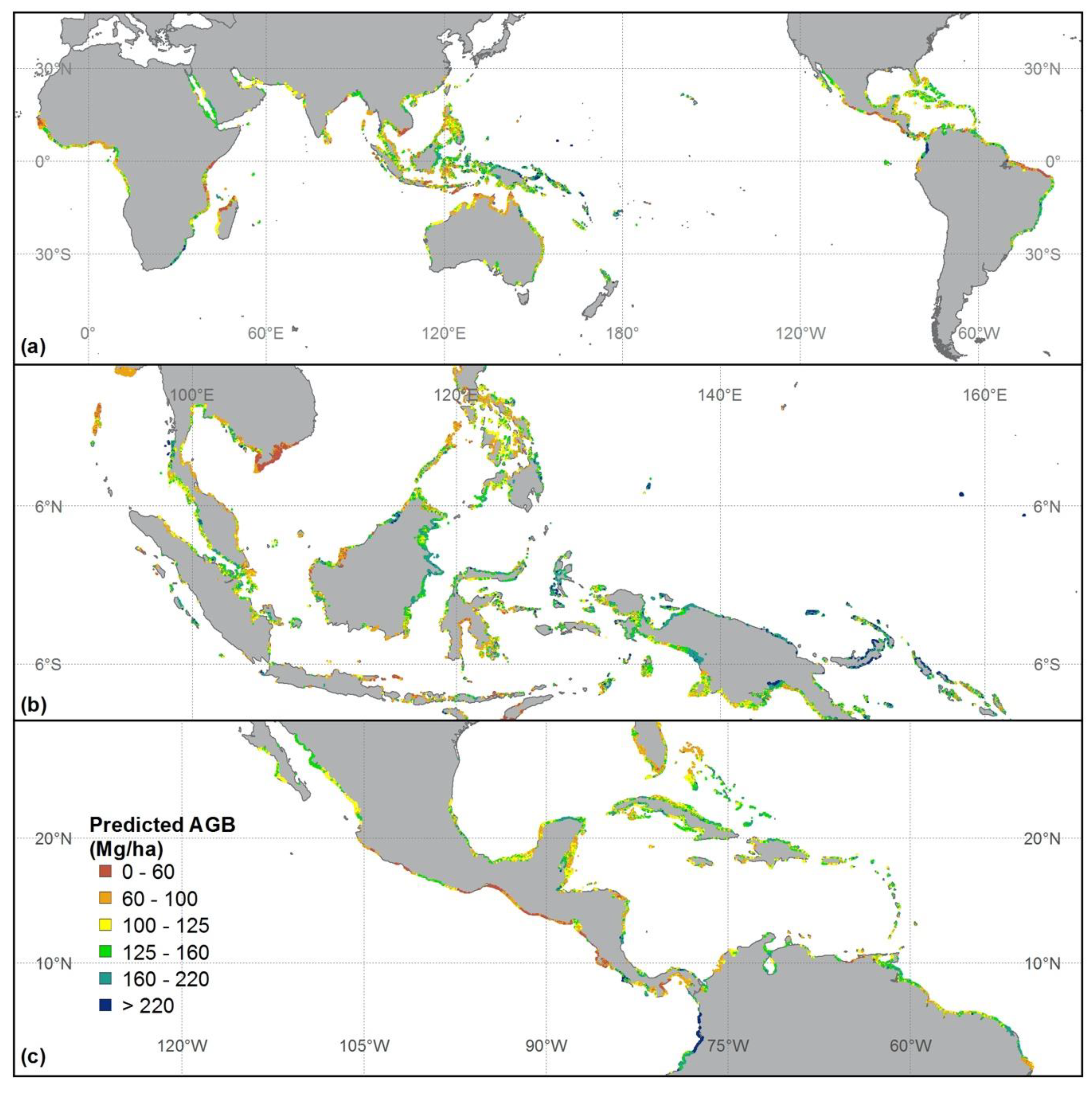
We used a random forest regression model with the three extrapolated GLAS parameters and other predictor variables to estimate global mangrove AGB. The random forest model explained 52.34% of the variance in AGB. The final AGB distribution pattern is similar to that of the GLAS parameters (Figure 4). The mean AGB density of global mangrove was 115.23 Mg/ha with a standard deviation of 48.89 Mg/ha. This map of AGB for mangrove forests will be shared on the GUO-Lab website (http://www.3decology.org).
3.3. Continental and National Level Mangrove Forest AGB Density
Total global AGB for mangroves was 1.52 Pg (Table 2), but the contribution by region was not uniform. Southeastern Asia provided 34.98% of the AGB (0.53 Pg) while having both the largest area (4,044,906.25 ha) and high AGB density (131.36 ± 45.94 Mg/ha). South America encompassed the second largest area (2,062,231.25 ha) and high AGB density (111.33 ± 58.70 Mg/ha), and the second highest stock of AGB (0.15 Pg). The mangrove AGB density in Central America (110.29 ± 39.48 Mg/ha) was similar to that of South America, although the area of mangrove in Central America was much smaller (1,388,962.50 ha). Mangrove AGB stocks in Southern Asia (0.13 Pg) and Western Africa (0.12 Pg) were similar, although the density of AGB was much higher in Southern Asia (132.6 ± 29.79 Mg/ha) than in Western Africa (79.27 ± 34.32 Mg/ha). The extent of mangrove in Southern Asia (949,281.25 ha), on the other hand, was lower than that in Western Africa (1,475,343.75 ha). At the national level, Indonesia had the highest stock of AGB (0.36 Pg) because of the high AGB density (140.12 ± 41.02 Mg/ha) and large area covered by mangrove (2,547,556.25 ha). Mexico had the second largest AGB (0.1 Pg) since it has large areas (891,312.50 ha) and high AGB density (113.98 ± 34.10 Mg/ha). The mangrove AGB density and stock for other important regions and countries are listed in Table 2.
3.4. The Accuracy of Mangrove AGB Estimation
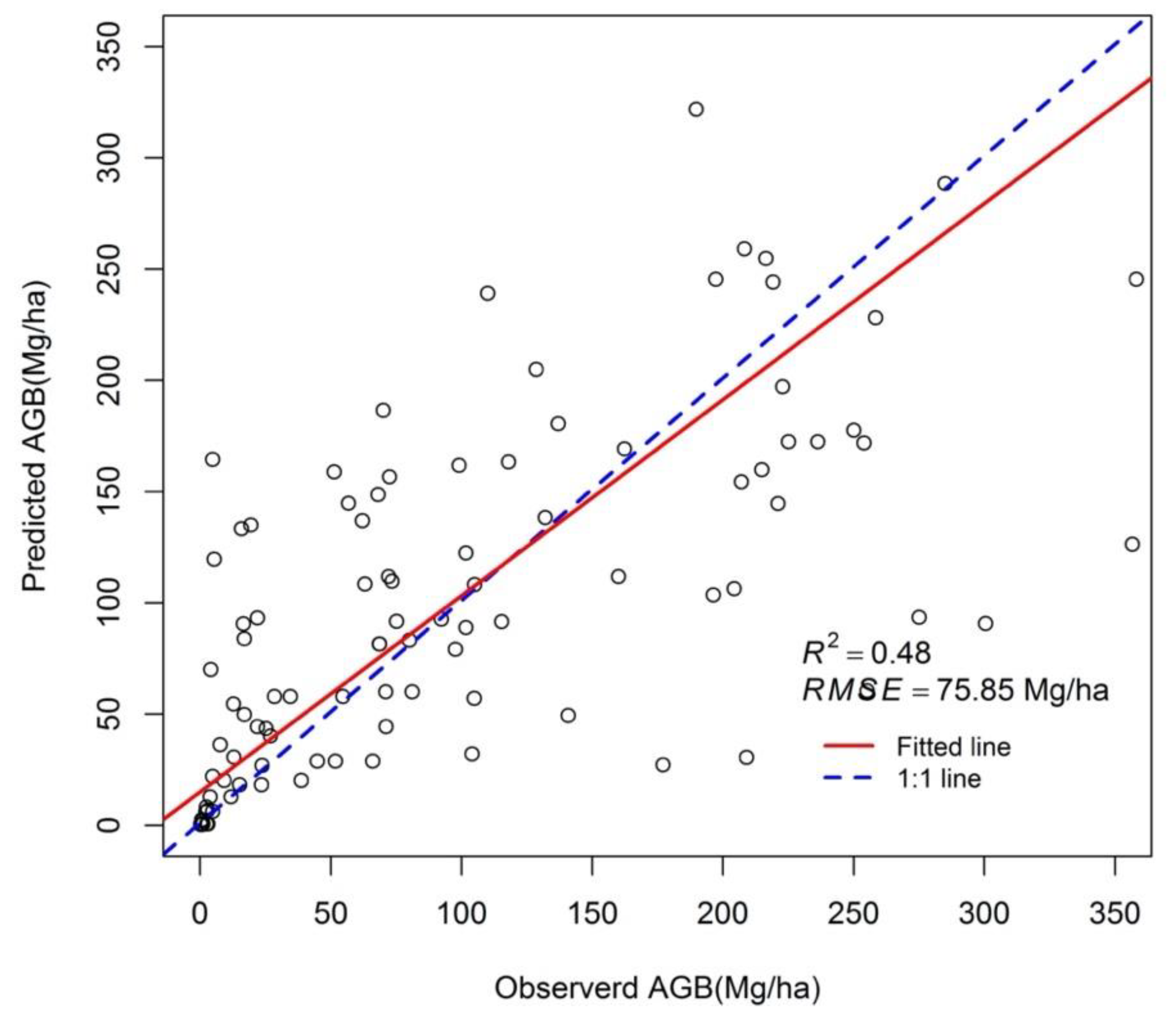
These estimates of mangrove AGB were validated using 103 independent validation plots (Figure 5). Predicted mangrove AGB was consistent with observerd AGB. The R2 between predicted and observed AGB is 0.48 and the RMSE is 75.85 Mg/ha. The AGB estimation method in this study tended to marginally overestimate AGB densities at low values (<125 Mg/ha; Figure 5) and tends to underestimate forest AGB density at high values (>125 Mg/ha).
4. Discussion
4.1. Comparison with Other Mangrove Models
Combining multi-source remote sensing data and surface observations helps us better understand global distribution of mangrove AGB. The model developed during this study is better able to explain the spatial variability in mangrove AGB (R2 = 0.48) than those of other models. Rovai et al. [33] developed a set of statistical climatic-geophysical models based on the environmental signature hypothesis, which explained only 20% of the variability in mangrove AGB in the Neotropics. Twilley et al.’s [31] latitude-based model explained 7.6% of the variation in mangrove AGB at the global scale, while Hutchison et al.’s [32] climate-based model explained 26.7% of the variation. We used our plot data to test Twilley et al.’s latitude-based model and Hutchison et al.’s [32] climate-based model; the resulting explanatory power of these two models was much lower at 2.2% and 10.5%, respectively. There are three primary reasons. First, the initial mangrove AGB dataset was extremely small in both Twilley et al.’s (n = 34) and Hutchison et al.’s (n = 52) analyses. Insufficient training data cannot be used to create a robust global scale model. These models, therefore, have large uncertainty when validated against our larger, global data set (n = 342).
Second, machine learning methods are more suitable to estimating global mangrove AGB than multi-linear regression methods. Although the climate variables used in our model and Hutchison et al.’s [32] climate-based model were similar, the explanatory power of our model was greater because of the difference in regression methods. Several studies have demonstrated that random forest performs better than the linear regression method for estimating biomass [64].
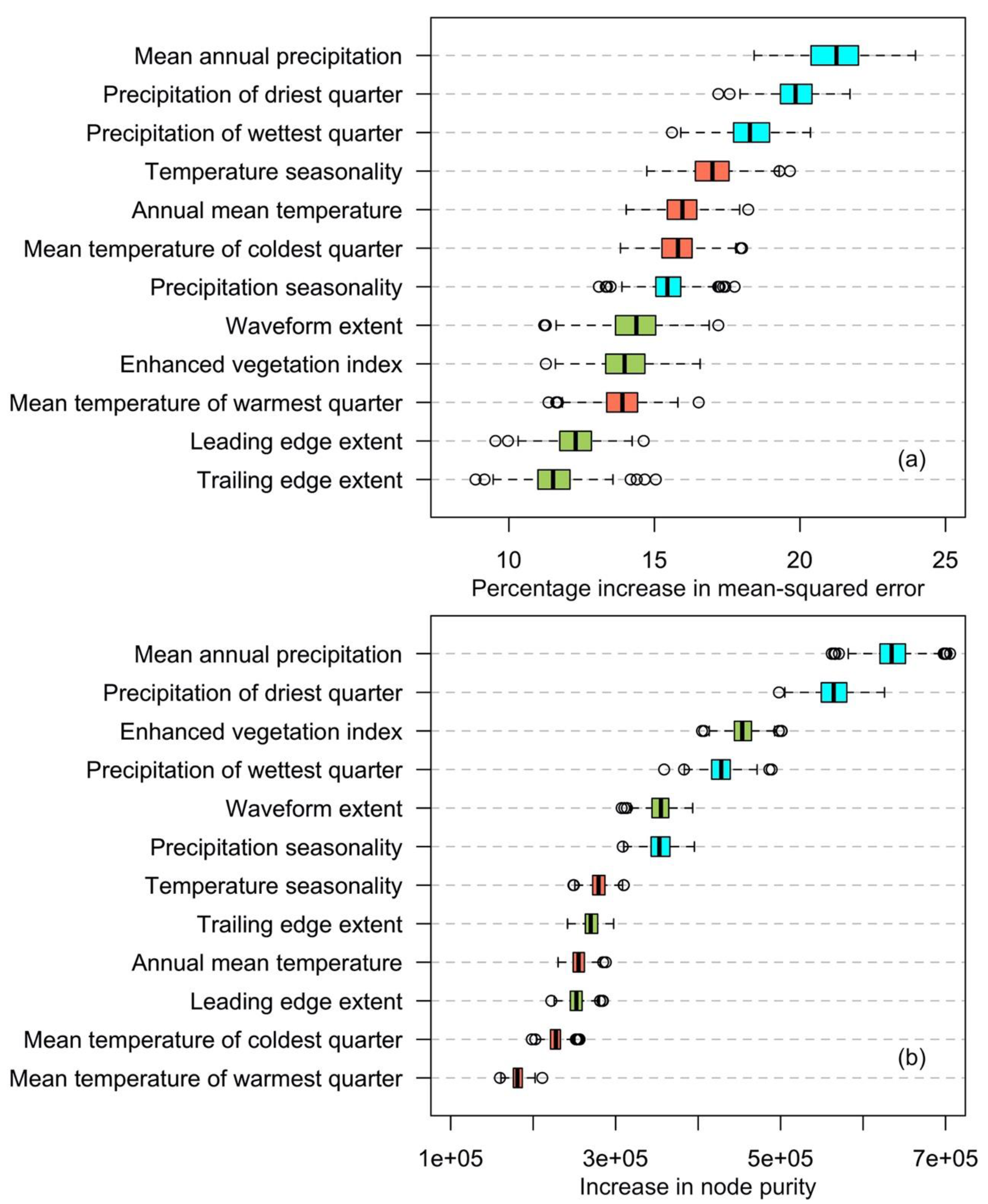
Finally, structural information provided by GLAS and EVI improved the accuracy of random forest to estimate mangrove AGB biomass (Figure 6). Recent field studies have found that canopy height is strongly related to biomass for many mangrove species [65,66]. However, structure information provided by GLAS does not have the expected effects in this study when compared with other research into national and global forest AGB mapping. This may have been caused by the low-density footprint of GLAS in mangrove areas, limiting its ability to represent the structure variation in different mangrove species. Based on the statistical importance of each variable in our model (Figure 6), climate factors were more important than other variables. This is similar to Simard et al.’s results in which precipitation, temperature and cyclone frequency explain 74% of the global variation in maximum canopy height [53].
4.2. Comparison with Previously Published Mangrove AGB Maps
Our estimated global mangrove AGB (1.52 Pg) was similar to that of two global maps produced using other remote sensing approaches (Table 3). Tang et al. [52] reported that total global mangrove AGB was 1.908 Pg, while Simard et al. [53] estimated it to be 1.75 Pg. Although the estimated mangrove storage was similar between these three remote sensing approaches, mean AGB density (115.23 ± 48.89 Mg/ha) in our study was lower than that of Tang et al. (146.3 Mg/ha) or Simard et al. (129.1 ± 87.2 Mg/ha). These differences are mainly caused by uncertainties induced by the allometric equations. Tang et al. [52] and Simard et al. [53] predicted global mangrove biomass using SRTM’s tree height and a global mangrove biomass allometry equation. The mean AGB density reported by Tang et al. was the highest of these three estimates. Compared to Saenger and Snedaker’s global mangrove height-biomass relationship used by Tang et al. [52], Simard et al. [53] applied 331 in situ plots across a wide variety of mangrove forest ecotypes to fit a global equation between AGB and basal area-weighted height. Our results for global mangrove AGB storage and mean AGB density were similar to that of Simard et al. [53] because both methods utilized spaceborne LiDAR data. Traditionally, mangrove forest aboveground biomass derived using synthetic aperture radar was underestimated due to its limited ability to penetrate the mangrove canopy. Simard et al. [53] used GLAS data to correct the SRTM tree height, thereby overcoming the issue of estimating mangrove AGB from SRTM tree height.
The estimated global mangrove AGB storage in our study (1.52 Pg) was significantly lower than those from non-remote sensing approaches (Table 3). Twilley et al. [31] estimated global mangrove AGB at 2.34 Pg based on a latitude model, nearly 54% higher than our result. Hutchison et al. [32] used a climate-based model and predicted that total global mangrove AGB storage was 2.83 Pg, 86% higher than our result. The difference in the baseline mangrove extent could be a major reason for the variation in these results. Although our study and that of Hutchison et al. [32] both used the mangrove map developed by Spalding et al. [19], the final global mangrove area in our study (13,065,675.00 ha) was 15% smaller than that used by Hutchison et al. [32] (15,314,094 ha). This difference was caused, in part, by inconsistent land boundaries between our predictor variables, mangrove distribution map, and country extents. These layers have different spatial resolutions and extents, so small mangrove patches along the coast or in the islets were omitted during our analysis. These places are also areas with a large distribution of mangrove [19]. Consequently, the disparity in area led to variations in total mangrove AGB storage between the two results. Part of the variation can also be explained by the models used by Hutchison et al., which may overestimate mangrove AGB [32]. Rovai et al. [33] found that these climate- and latitude-based models overestimated mangrove AGB by 25.3% to 44.4% in the Neotropics region. In addition, the structural data provided by spaceborne LiDAR in this study can provide better information for estimating mangrove AGB at larger geographical scales, thereby reducing uncertainty in estimates of mangrove AGB storage.
Most of the 10 countries with largest total mangrove AGB stock from our study were also reported in other research, such as that of Hutchison et al. (2014) [32] and Simard et al. (2019) [53], but the order in which these countries appear on the list was different. Indonesia has the largest mangrove AGB stock, which is consist in each study, even though the mangrove AGB in Indonesia and Papua New Guinea reported by our study was much lower than those of Hutchison et al. (2014) [32] and Simard et al. (2019) [53] (Figure 7). This phenomenon maybe caused by the model we used to predict biomass. Validation (Figure 5) showed that our model tended to underestimate mangrove AGB density at high values (>125 Mg/ha) since observations are limited in these high biomass areas. The mangrove AGB stock in Mexico, Cuba, and Colombia differed between the three studies. The difference in Mexico and Cuba was induced by a bias in predicted mean mangrove AGB density in the different studies. Adame et al. (2013) reported that the AGB in tall, medium and dwarf mangroves in the Mexican Caribbean were as much as 176.2, 114.2 and 7.1 Mg/ha, respectively [68]. The mean mangrove AGB density of Mexico in our study was 113.30 Mg/ha which is closer to that of the medium mangroves reported by Adame et al. (2013). Simard et al. (2019) [53] reported a mean AGB in Mexico of 37.9 Mg/ha, which is much lower than that of the medium mangroves. This underestimation in Simard et al. (2019) [53] may have been caused by using a global allometric equation to predict biomass. The difference in Colombia was mainly caused by inconsistencies in mangrove extent. The mangrove area in Colombia reported by Simard et al. (2019) [53] is much lower than that in our study and in Hutchison et al. (2014) [32].
4.3. Limitations and Future Studies
Although our model estimates global mangrove aboveground biomass fairly well, there are limitations to this study. Available observation data was limited when compared with other regional and global studies. Field data is fundamental for accurate estimations of global mangrove biomass. In this study, we collected 510 records from a number of sources but more than 30% of them could not be used because of uncertainty in location information. Moreover, geolocation errors in mangrove plots cannot be reduced by the point-radius model used by Su et al. [47] and Hu et al. [46], because randomly shifting mangrove plot locations had a large probability of relocating the plot into the ocean. Furthermore, the mismatch of spatial observation scales between plots and remote sensing data was a problem. Researchers have begun recently to use drone-based LiDAR to retrieve mangrove biomass [69], using it as a bridge to scale AGB from the plot level to the scale of satellite observations [70]. The increase in drone-based LiDAR data in mangrove areas will benefit global mangrove forest biomass mapping efforts in the future. Second, sparse GLAS datapoints within areas of mangrove lose some of the variability in structure during extrapolation. Even though we used GLAS data within a 100-km buffer of the coast to increase the number of GLAS datapoints, the explanatory power of the extrapolation models were nearly 10% lower than those for China and global forest mapping [46,47]. Fortunately, the Global Ecosystem Dynamics Investigation (GEDI) project [71] recently started collecting global waveform LiDAR data, which will provide higher density data with a smaller footprint than GLAS. This data will help us better understand variability in mangrove structure and biomass distribution. Third, factors such as salinity [72] and river discharge [73] that specifically control the distribution and production of mangrove forest should be added to the model in the future. With these factors, we can more accurately estimate the biomass and better understand how mangrove AGB varies under different environmental conditions.
5. Conclusions
This study produced a new global estimate of mangrove AGB for the year 2004, resulting in a 250-m resolution map that will be publicly available (http://www.3decology.org). This product was generated using methodology that was successfully implemented previously to estimate nation-wide forest AGB for China as well as global forest AGB. Three GLAS parameters and an additional nine predictor variables were used to build a random forest estimation model using plot measurements collected from published literature and free-access datasets. Based on this mangrove AGB analysis, global mangrove AGB density was estimated to be approximately 115.67 (±48.89) Mg/ha on average, with a total global AGB for mangrove forests of 1.52 Pg. Our product was compared to published global mangrove AGB products, and it has better explanatory power (R2 = 0.48, RMSE = 75.85 Mg/ha) than previous climate-based models. Results showed that this estimated global mangrove AGB storage was similar to that predicted by other remote sensing methods, especially the mangrove AGB map produced by Simard et al. [53]. Future research will include better LiDAR-based measurements of mangrove biomass as well as additional factors known to affect mangrove distribution.
Author Contributions
Conceptualization, T.H., Y.Z. (YingYing Zhang), Y.S. and Q.G.; Data curation, T.H., Y.Z. (YingYing Zhang), Y.Z. (Yi Zheng) and G.L.; Formal analysis, T.H., Y.Z. (YingYing Zhang) and Y.S.; Writing—original draft, T.H. and Y.Z. (YingYing Zhang); Writing—review & editing, T.H., Y.S. and Q.G. All authors have read and agreed to the published version of the manuscript.
Funding
This study Supported by the National Key R&D Program of China (2017YFC0503905).
Acknowledgments
Thanks to the Center for International Forestry Research (CIFOR, https://www.cifor.org/) for providing mangrove field data.
Conflicts of Interest
The authors declare no conflict of interest.
References
- Alongi, D.M. Present state and future of the world’s mangrove forests. Environ. Conserv. 2002, 29, 331–349. [Google Scholar] [CrossRef] [Green Version]
- Mazda, Y.; Wolanski, E.; Ridd, P. The Role of Physical Processes in Mangrove Environments: Manual for the Preservation and Utilization of Mangrove Ecosystems; Terrapub: Tokyo, Japan, 2007. [Google Scholar]
- Lee, S.Y.; Primavera, J.H.; Dahdouh-Guebas, F.; McKee, K.; Bosire, J.O.; Cannicci, S.; Diele, K.; Fromard, F.; Koedam, N.; Marchand, C.; et al. Ecological role and services of tropical mangrove ecosystems: A reassessment. Glob. Ecol. Biogeogr. 2014, 23, 726–743. [Google Scholar] [CrossRef]
- Alongi, D.M. Mangrove forests: Resilience, protection from tsunamis, and responses to global climate change. Estuar. Coast. Shelf Sci. 2008, 76, 1–13. [Google Scholar] [CrossRef]
- Bouillon, S.; Borges, A.V.; Castañeda-Moya, E.; Diele, K.; Dittmar, T.; Duke, N.C.; Kristensen, E.; Lee, S.Y.; Marchand, C.; Middelburg, J.J.; et al. Mangrove production and carbon sinks: A revision of global budget estimates. Glob. Biogeochem. Cycles 2008, 22. [Google Scholar] [CrossRef] [Green Version]
- Alongi, D.M.; Mukhopadhyay, S.K. Contribution of mangroves to coastal carbon cycling in low latitude seas. Agric. For. Meteorol. 2015, 213, 266–272. [Google Scholar] [CrossRef]
- Giri, C.; Ochieng, E.; Tieszen, L.L.; Zhu, Z.; Singh, A.; Loveland, T.; Masek, J.; Duke, N. Status and distribution of mangrove forests of the world using earth observation satellite data: Status and distributions of global mangroves. Glob. Ecol. Biogeogr. 2011, 20, 154–159. [Google Scholar] [CrossRef]
- Donato, D.C.; Kauffman, J.B.; Murdiyarso, D.; Kurnianto, S.; Stidham, M.; Kanninen, M. Mangroves among the most carbon-rich forests in the tropics. Nat. Geosci. 2011, 4, 293. [Google Scholar] [CrossRef]
- Tomlinson, P. Mangrove Botany; Cambridge Univ. Press: Cambridge, UK, 1986. [Google Scholar]
- Ellison, A.M.; Farnsworth, E.J.; Merkt, R.E. Origins of mangrove ecosystems and the mangrove biodiversity anomaly. Glob. Ecol. Biogeogr. 1999, 8, 95–115. [Google Scholar] [CrossRef] [Green Version]
- Duke, N.; Ball, M.; Ellison, J. Factors influencing biodiversity and distributional gradients in mangroves. Glob. Ecol. Biogeogr. Lett. 1998, 7, 27–47. [Google Scholar] [CrossRef] [Green Version]
- Nagelkerken, I.; Blaber, S.; Bouillon, S.; Green, P.; Haywood, M.; Kirton, L.; Meynecke, J.-O.; Pawlik, J.; Penrose, H.; Sasekumar, A. The habitat function of mangroves for terrestrial and marine fauna: A review. Aquat. Bot. 2008, 89, 155–185. [Google Scholar] [CrossRef] [Green Version]
- Buelow, C.; Sheaves, M. A birds-eye view of biological connectivity in mangrove systems. Estuar. Coast. Shelf Sci. 2015, 152, 33–43. [Google Scholar] [CrossRef]
- Mumby, P.J.; Edwards, A.J.; Ernesto Arias-González, J.; Lindeman, K.C.; Blackwell, P.G.; Gall, A.; Gorczynska, M.I.; Harborne, A.R.; Pescod, C.L.; Renken, H.; et al. Mangroves enhance the biomass of coral reef fish communities in the Caribbean. Nature 2004, 427, 533. [Google Scholar] [CrossRef] [PubMed] [Green Version]
- Ward, R.D.; Friess, D.A.; Day, R.H.; MacKenzie, R.A. Impacts of climate change on mangrove ecosystems: A region by region overview. Ecosyst. Health Sustain. 2016, 2, e01211. [Google Scholar] [CrossRef] [Green Version]
- Krauss, K.W.; McKee, K.L.; Lovelock, C.E.; Cahoon, D.R.; Saintilan, N.; Reef, R.; Chen, L. How mangrove forests adjust to rising sea level. New Phytol. 2014, 202, 19–34. [Google Scholar] [CrossRef] [PubMed] [Green Version]
- Valiela, I.; Bowen, J.L.; York, J.K. Mangrove Forests: One of the World’s Threatened Major Tropical Environments: At least 35% of the area of mangrove forests has been lost in the past two decades, losses that exceed those for tropical rain forests and coral reefs, two other well-known threatened environments. BioScience 2001, 51, 807–815. [Google Scholar] [CrossRef] [Green Version]
- McLeod, E.; Chmura, G.L.; Bouillon, S.; Salm, R.; Björk, M.; Duarte, C.M.; Lovelock, C.E.; Schlesinger, W.H.; Silliman, B.R. A blueprint for blue carbon: Toward an improved understanding of the role of vegetated coastal habitats in sequestering CO2. Front. Ecol. Environ. 2011, 9, 552–560. [Google Scholar] [CrossRef] [Green Version]
- Spalding, M. World Atlas of Mangroves; Routledge: London, UK, 2010. [Google Scholar] [CrossRef]
- FAO. The World’s Mangroves 1980–2005; Food and Agriculture Organization: Rome, Italy, 2007. [Google Scholar]
- Thomas, N.; Lucas, R.; Bunting, P.; Hardy, A.; Rosenqvist, A.; Simard, M. Distribution and drivers of global mangrove forest change, 1996–2010. PLoS ONE 2017, 12, e0179302. [Google Scholar] [CrossRef] [Green Version]
- Zhila, H.; Mahmood, H.; Rozainah, M.Z. Biodiversity and biomass of a natural and degraded mangrove forest of Peninsular Malaysia. Environ. Earth Sci. 2014, 71, 4629–4635. [Google Scholar] [CrossRef]
- Tamai, S.; Nakasuga, T.; Tabuchi, R.; Ogino, K. Standing Biomass of Mangrove Forests in Southern Thailand. J. Jpn. For. Soc. 1986, 68, 384–388. [Google Scholar] [CrossRef]
- Slim, F.J.; Gwada, P.M.; Kodjo, M.; Hemminga, M.A. Biomass and litterfall of Ceriops tagal and Rhizophora mucronata in the mangrove forest of Gazi Bay, Kenya. Mar. Freshw. Res. 1996, 47, 999–1007. [Google Scholar] [CrossRef]
- Ross, M.S.; Ruiz, P.L.; Telesnicki, G.J.; Meeder, J.F. Estimating above-ground biomass and production in mangrove communities of Biscayne National Park, Florida (U.S.A.). Wetl. Ecol. Manag. 2001, 9, 27–37. [Google Scholar] [CrossRef]
- Soares, M.L.G.; Schaeffer-Novelli, Y. Above-ground biomass of mangrove species. I. Analysis of models. Estuar. Coast. Shelf Sci. 2005, 65, 1–18. [Google Scholar] [CrossRef]
- Komiyama, A.; Ong, J.E.; Poungparn, S. Allometry, biomass, and productivity of mangrove forests: A review. Aquat. Bot. 2008, 89, 128–137. [Google Scholar] [CrossRef]
- Chandra, I.A.; Seca, G.; Hena, M.K.A. Aboveground Biomass Production of Rhizophora apiculata Blume in Sarawak Mangrove Forest. Am. J. Agric. Biol. Sci. 2011, 6, 469–474. [Google Scholar]
- Mitra, A.; Sengupta, K.; Banerjee, K. Standing biomass and carbon storage of above-ground structures in dominant mangrove trees in the Sundarbans. For. Ecol. Manag. 2011, 261, 1325–1335. [Google Scholar] [CrossRef]
- Comley, B.W.T.; McGuinness, K.A. Above- and below-ground biomass, and allometry, of four common northern Australian mangroves. Aust. J. Bot. 2005, 53, 431–436. [Google Scholar] [CrossRef]
- Twilley, R.R.; Chen, R.H.; Hargis, T. Carbon sinks in mangroves and their implications to carbon budget of tropical coastal ecosystems. Water Air Soil Pollut. 1992, 64, 265–288. [Google Scholar] [CrossRef]
- Hutchison, J.; Manica, A.; Swetnam, R.; Balmford, A.; Spalding, M. Predicting Global Patterns in Mangrove Forest Biomass. Conserv. Lett. 2014, 7, 233–240. [Google Scholar] [CrossRef] [Green Version]
- Rovai, A.S.; Riul, P.; Twilley, R.R.; Castañeda-Moya, E.; Rivera-Monroy, V.H.; Williams, A.A.; Simard, M.; Cifuentes-Jara, M.; Lewis, R.R.; Crooks, S.; et al. Scaling mangrove aboveground biomass from site-level to continental-scale: Scaling up mangrove AGB from site- to continental-level. Glob. Ecol. Biogeogr. 2016, 25, 286–298. [Google Scholar] [CrossRef]
- Heumann, B.W. Satellite remote sensing of mangrove forests: Recent advances and future opportunities. Prog. Phys. Geogr. Earth Environ. 2011, 35, 87–108. [Google Scholar] [CrossRef]
- Proisy, C.; Couteron, P.; Fromard, F. Predicting and mapping mangrove biomass from canopy grain analysis using Fourier-based textural ordination of IKONOS images. Remote Sens. Environ. 2007, 109, 379–392. [Google Scholar] [CrossRef]
- Wang, L.; Jia, M.; Yin, D.; Tian, J. A review of remote sensing for mangrove forests: 1956–2018. Remote Sens. Environ. 2019, 231, 111223. [Google Scholar] [CrossRef]
- Simard, M.; Zhang, K.; Rivera-Monroy, V.H.; Ross, M.S.; Ruiz, P.L.; Castañeda-Moya, E.; Twilley, R.R.; Rodriguez, E. Mapping Height and Biomass of Mangrove Forests in Everglades National Park with SRTM Elevation Data. Photogramm. Eng. Remote Sens. 2006, 72, 299–311. [Google Scholar] [CrossRef]
- Pham, T.D.; Yokoya, N.; Bui, D.T.; Yoshino, K.; Friess, D.A. Remote Sensing Approaches for Monitoring Mangrove Species, Structure, and Biomass: Opportunities and Challenges. Remote Sens. 2019, 11, 230. [Google Scholar] [CrossRef] [Green Version]
- Lu, D. The potential and challenge of remote sensing-based biomass estimation. Int. J. Remote Sens. 2006, 27, 1297–1328. [Google Scholar] [CrossRef]
- Lim, K.; Treitz, P.; Wulder, M.; St-Onge, B.; Flood, M. LiDAR remote sensing of forest structure. Prog. Phys. Geogr. Earth Environ. 2003, 27, 88–106. [Google Scholar] [CrossRef] [Green Version]
- Zimble, D.A.; Evans, D.L.; Carlson, G.C.; Parker, R.C.; Grado, S.C.; Gerard, P.D. Characterizing vertical forest structure using small-footprint airborne LiDAR. Remote Sens. Environ. 2003, 87, 171–182. [Google Scholar] [CrossRef] [Green Version]
- Babcock, C.; Finley, A.O.; Bradford, J.B.; Kolka, R.; Birdsey, R.; Ryan, M.G. LiDAR based prediction of forest biomass using hierarchical models with spatially varying coefficients. Remote Sens. Environ. 2015, 169, 113–127. [Google Scholar] [CrossRef] [Green Version]
- Dubayah, R.O.; Drake, J.B. Lidar Remote Sensing for Forestry. J. For. 2000, 98, 44–46. [Google Scholar] [CrossRef]
- Clark, M.L.; Roberts, D.A.; Ewel, J.J.; Clark, D.B. Estimation of tropical rain forest aboveground biomass with small-footprint lidar and hyperspectral sensors. Remote Sens. Environ. 2011, 115, 2931–2942. [Google Scholar] [CrossRef]
- Næsset, E.; Gobakken, T.; Solberg, S.; Gregoire, T.G.; Nelson, R.; Ståhl, G.; Weydahl, D. Model-assisted regional forest biomass estimation using LiDAR and InSAR as auxiliary data: A case study from a boreal forest area. Remote Sens. Environ. 2011, 115, 3599–3614. [Google Scholar] [CrossRef]
- Hu, T.; Su, Y.; Xue, B.; Liu, J.; Zhao, X.; Fang, J.; Guo, Q. Mapping Global Forest Aboveground Biomass with Spaceborne LiDAR, Optical Imagery, and Forest Inventory Data. Remote Sens. 2016, 8, 565. [Google Scholar] [CrossRef] [Green Version]
- Su, Y.; Guo, Q.; Xue, B.; Hu, T.; Alvarez, O.; Tao, S.; Fang, J. Spatial distribution of forest aboveground biomass in China: Estimation through combination of spaceborne lidar, optical imagery, and forest inventory data. Remote Sens. Environ. 2016, 173, 187–199. [Google Scholar] [CrossRef] [Green Version]
- Lefsky, M.A. A global forest canopy height map from the Moderate Resolution Imaging Spectroradiometer and the Geoscience Laser Altimeter System. Geophys. Res. Lett. 2010, 37. [Google Scholar] [CrossRef] [Green Version]
- Simard, M.; Pinto, N.; Fisher, J.B.; Baccini, A. Mapping forest canopy height globally with spaceborne lidar. J. Geophys. Res. Biogeosci. 2011, 116. [Google Scholar] [CrossRef]
- Baccini, A.; Goetz, S.J.; Walker, W.S.; Laporte, N.T.; Sun, M.; Sulla-Menashe, D.; Hackler, J.; Beck, P.S.A.; Dubayah, R.; Friedl, M.A.; et al. Estimated carbon dioxide emissions from tropical deforestation improved by carbon-density maps. Nat. Clim. Chang. 2012, 2, 182. [Google Scholar] [CrossRef]
- Boudreau, J.; Nelson, R.F.; Margolis, H.A.; Beaudoin, A.; Guindon, L.; Kimes, D.S. Regional aboveground forest biomass using airborne and spaceborne LiDAR in Québec. Remote Sens. Environ. 2008, 112, 3876–3890. [Google Scholar] [CrossRef]
- Tang, W.; Zheng, M.; Zhao, X.; Shi, J.; Yang, J.; Trettin, C.C. Big Geospatial Data Analytics for Global Mangrove Biomass and Carbon Estimation. Sustainability 2018, 10, 472. [Google Scholar] [CrossRef] [Green Version]
- Simard, M.; Fatoyinbo, L.; Smetanka, C.; Rivera-Monroy, V.H.; Castañeda-Moya, E.; Thomas, N.; Stocken, T.V.D. Mangrove canopy height globally related to precipitation, temperature and cyclone frequency. Nat. Geosci. 2019, 12, 40–45. [Google Scholar] [CrossRef]
- Hijmans, R.J.; Cameron, S.E.; Parra, J.L.; Jones, P.G.; Jarvis, A. Very high resolution interpolated climate surfaces for global land areas. Int. J. Climatol. 2005, 25, 1965–1978. [Google Scholar] [CrossRef]
- Zhao, X.; Su, Y.; Hu, T.; Chen, L.; Gao, S.; Wang, R.; Jin, S.; Guo, Q. A global corrected SRTM DEM product for vegetated areas. Remote Sens. Lett. 2018, 9, 393–402. [Google Scholar] [CrossRef]
- Huete, A.; Justice, C.; Van Leeuwen, W. MODIS vegetation index (MOD13). Algorithm Theor. Basis Doc. 1999, 3, 213. [Google Scholar]
- Murdiyarso, D.; Purbopuspito, J.; Kauffman, J.B.; Warren, M.W.; Sasmito, S.D.; Manuri, S.; Krisnawati, H.; Taberima, S.; Kurnianto, S. SWAMP Dataset-Mangrove Biomass Vegetation-Teminabuan-2011, V1 ed.; Center for International Forestry Research (CIFOR): Bogor, Indonesia, 2019. [Google Scholar] [CrossRef]
- Sasmito, S.D.; Silanpää, M.; Hayes, M.A.; Bachri, S.; Saragi-Sasmito, M.F.; Sidik, F.; Hanggara, B.; Mofu, W.Y.; Rumbiak, V.I.; Hendri; et al. SWAMP Dataset-Mangrove Necromass-West Papua-2019, DRAFT VERSION ed.; Center for International Forestry Research (CIFOR): Bogor, Indonesia, 2019. [Google Scholar] [CrossRef]
- Zwally, H.J.; Schutz, B.; Abdalati, W.; Abshire, J.; Bentley, C.; Brenner, A.; Bufton, J.; Dezio, J.; Hancock, D.; Harding, D.; et al. ICESat’s laser measurements of polar ice, atmosphere, ocean, and land. J. Geodyn. 2002, 34, 405–445. [Google Scholar] [CrossRef] [Green Version]
- Lefsky, M.A.; Keller, M.; Pang, Y.; De Camargo, P.B.; Hunter, M.O. Revised method for forest canopy height estimation from Geoscience Laser Altimeter System waveforms. J. Appl. Remote Sens. 2007, 1, 013537. [Google Scholar] [CrossRef]
- Scholes, R.J.; Kendall, J.; Justice, C.O. The quantity of biomass burned in southern Africa. J. Geophys. Res. Atmos. 1996, 101, 23667–23676. [Google Scholar] [CrossRef]
- Li, L.; Guo, Q.; Tao, S.; Kelly, M.; Xu, G. Lidar with multi-temporal MODIS provide a means to upscale predictions of forest biomass. ISPRS J. Photogramm. Remote Sens. 2015, 102, 198–208. [Google Scholar] [CrossRef]
- Liaw, A.; Wiener, M. Classification and regression by randomForest. R News 2002, 2, 18–22. [Google Scholar]
- Fassnacht, F.E.; Hartig, F.; Latifi, H.; Berger, C.; Hernández, J.; Corvalán, P.; Koch, B. Importance of sample size, data type and prediction method for remote sensing-based estimations of aboveground forest biomass. Remote Sens. Environ. 2014, 154, 102–114. [Google Scholar] [CrossRef]
- Fromard, F.; Puig, H.; Mougin, E.; Marty, G.; Betoulle, J.L.; Cadamuro, L. Structure, above-ground biomass and dynamics of mangrove ecosystems: New data from French Guiana. Oecologia 1998, 115, 39–53. [Google Scholar] [CrossRef]
- Smith, T.J.; Whelan, K.R.T. Development of allometric relations for three mangrove species in South Florida for use in the Greater Everglades Ecosystem restoration. Wetl. Ecol. Manag. 2006, 14, 409–419. [Google Scholar] [CrossRef]
- World Resources Institute; International Institute for Environment and Development. World Resources 1986. In An Assessment of the Resources Base That Supports the Global Economy; Basic Books: New York, NY, USA, 1986. [Google Scholar]
- Adame, M.F.; Kauffman, J.B.; Medina, I.; Gamboa, J.N.; Torres, O.; Caamal, J.P.; Reza, M.; Herrera-Silveira, J.A. Carbon Stocks of Tropical Coastal Wetlands within the Karstic Landscape of the Mexican Caribbean. PLoS ONE 2013, 8, e56569. [Google Scholar] [CrossRef] [PubMed] [Green Version]
- Guo, Q.; Su, Y.; Hu, T.; Zhao, X.; Wu, F.; Li, Y.; Liu, J.; Chen, L.; Xu, G.; Lin, G.; et al. An integrated UAV-borne lidar system for 3D habitat mapping in three forest ecosystems across China. Int. J. Remote Sens. 2017, 38, 2954–2972. [Google Scholar] [CrossRef]
- Zhu, X.; Hou, Y.; Weng, Q.; Chen, L. Integrating UAV optical imagery and LiDAR data for assessing the spatial relationship between mangrove and inundation across a subtropical estuarine wetland. ISPRS J. Photogramm. Remote Sens. 2019, 149, 146–156. [Google Scholar] [CrossRef]
- Coyle, D.B.; Stysley, P.R.; Poulios, D.; Clarke, G.B.; Kay, R.B. Laser Transmitter Development for NASA’s Global Ecosystem Dynamics Investigation (GEDI) Lidar. In Proceedings of the SPIE—The International Society for Optics and Photonics, San Diego, CA, USA, 9–13 August 2015; Volume 9612, p. 7. [Google Scholar]
- Naidoo, G. Effects of salinity and nitrogen on growth and water relations in the mangrove, Avicennia marina (Forsk.) Vierh. New Phytol. 1987, 107, 317–325. [Google Scholar] [CrossRef]
- Wösten, J.H.M.; de Willigen, P.; Tri, N.H.; Lien, T.V.; Smith, S.V. Nutrient dynamics in mangrove areas of the Red River Estuary in Vietnam. Estuar. Coast. Shelf Sci. 2003, 57, 65–72. [Google Scholar] [CrossRef]
Figure 1.
The workflow for producing global mangrove aboveground biomass map based on the multisource remote sensing data and ground observation data.
Figure 1.
The workflow for producing global mangrove aboveground biomass map based on the multisource remote sensing data and ground observation data.

Figure 2.
The collected mangrove plots distribution across the world. The color of each point indicated the value of aboveground biomass.
Figure 2.
The collected mangrove plots distribution across the world. The color of each point indicated the value of aboveground biomass.

Figure 3.
The spatial-continuous map of three GLAS parameters in the mangrove distribution zone, (a) waveform extent, (b) leading edge extent, and (c) trailing edge extent. Note that the spatially continuous map was drawn using points since the mangrove distribution zone is narrow and cannot be represented well using a raster map at the global scale.

Figure 4.
Predicted mangrove forest AGB distribution (a) throughout the world, (b) enlarged over Southeastern Asia, and (c) enlarged over Central America.
Figure 4.
Predicted mangrove forest AGB distribution (a) throughout the world, (b) enlarged over Southeastern Asia, and (c) enlarged over Central America.

Figure 5.
The validation of mangrove biomass estimated model. R2 represents the adjusted coefficient of determination, RMSE represents the root-mean-square error.
Figure 5.
The validation of mangrove biomass estimated model. R2 represents the adjusted coefficient of determination, RMSE represents the root-mean-square error.

Figure 6.
The mean importance of variables for AGB estimation using the randomForest model is indicated by the percentage increase of mean-squared error (a) and the increase in node purity (b) from highest to lowest. Percentage increase in mean square error is calculated by the increase in mean square error when a variable is removed in the model. The increase in node purity is calculated based on the reduction in sum of squared errors whenever a variable is chosen to split.

Figure 7.
Comparison of (a) mean mangrove AGB density, (b) mangrove area, and (c) total mangrove AGB stock between our study, Hutchison et al. (2014) and Simard et al. (2019) in ten countries with the highest mangrove AGB.
Figure 7.
Comparison of (a) mean mangrove AGB density, (b) mangrove area, and (c) total mangrove AGB stock between our study, Hutchison et al. (2014) and Simard et al. (2019) in ten countries with the highest mangrove AGB.


Table 1.
The variables used in the random forest method to determine GLAS parameters and model mangrove aboveground biomass.
Table 1.
The variables used in the random forest method to determine GLAS parameters and model mangrove aboveground biomass.
| Variable | Dataset | Year | Resolution | Reference |
|---|---|---|---|---|
| Mean annual precipitation (mm) | Worldclim | 1950–2000 | 1 km | Hijmans et al., 2005 [54] |
| Precipitation of driest quarter (mm) | Worldclim | 1950–2000 | 1 km | Hijmans et al., 2005 [54] |
| Precipitation seasonality | Worldclim | 1950–2000 | 1 km | Hijmans et al., 2005 [54] |
| Precipitation of wettest quarter (mm) | Worldclim | 1950–2000 | 1 km | Hijmans et al., 2005 [54] |
| Annual mean temperature (°C) | Worldclim | 1950–2000 | 1 km | Hijmans et al., 2005 [54] |
| Mean temperature of driest quarter (°C) | Worldclim | 1950–2000 | 1 km | Hijmans et al., 2005 [54] |
| Mean temperature of warmest quarter (°C) | Worldclim | 1950–2000 | 1 km | Hijmans et al., 2005 [54] |
| Temperature seasonality | Worldclim | 1950–2000 | 1 km | Hijmans et al., 2005 [54] |
| Elevation (m) | CSRTM | 2000 | 30 m | Zhao et al., 2018 [55] |
| Slope | CSRTM | 2000 | 30 m | Zhao et al., 2018 [55] |
| Enhanced vegetation index (EVI) | MOD13Q1 | 2004 | 250 m | Huete et al., 1999 [56] |
| Waveform extent (m) | GLAS | 2004 | ~ a 70 m diameter spots | n/a |
| Leading edge extent (m) | GLAS | 2004 | ~ a 70 m diameter spots | n/a |
| Trailing edge extent (m) | GLAS | 2004 | ~ a 70 m diameter spots | n/a |
Table 2.
The mean AGB density and total AGB in the different regions and countries.
| Region * | Mean AGB (Mg/ha) | Mangrove Area (ha) | Total AGB (Mg) | Proportion of Global AGB (%) |
| Southeastern Asia | 131.36 ± 45.94 | 4,044,906.25 | 531,347,520.57 | 34.98 |
| South America | 111.33 ± 58.70 | 2,062,231.25 | 229,594,355.48 | 15.12 |
| Central America | 110.29 ± 39.48 | 1,388,962.50 | 153,185,736.15 | 10.09 |
| Southern Asia | 132.60 ± 29.79 | 949,281.25 | 125,874,227.46 | 8.29 |
| Western Africa | 79.27 ± 34.32 | 1,475,343.75 | 116,944,200.85 | 7.70 |
| Eastern Africa | 102.79 ± 53.63 | 821,906.25 | 84,482,779.41 | 5.56 |
| Caribbean | 123.69 ± 31.40 | 571,493.75 | 70,690,803.56 | 4.65 |
| Melanesia | 149.24 ± 48.63 | 438,768.75 | 65,479,984.29 | 4.31 |
| Australia and New Zealand | 101.22 ± 38.71 | 523,643.75 | 53,000,621.89 | 3.49 |
| Middle Africa | 101.79 ± 36.88 | 393,006.25 | 40,003,008.67 | 2.63 |
| Northern America | 103.48 ± 44.90 | 300,956.25 | 31,142,627.18 | 2.05 |
| Southern Africa | 197.16 ± 52.95 | 43,118.75 | 8,501,508.15 | 0.56 |
| Western Asia | 134.24 ± 16.11 | 23,162.50 | 3,109,444.89 | 0.20 |
| Micronesia | 279.89 ± 81.67 | 10,162.50 | 2,844,427.43 | 0.19 |
| Northern Africa | 161.37 ± 11.47 | 9,481.25 | 1,529,943.27 | 0.10 |
| Eastern Asia | 114.90 ± 23.41 | 9,156.25 | 1,052,045.89 | 0.07 |
| Polynesia | 160.25 ± 58.88 | 100.00 | 16,025.34 | <0.01 |
| Global | 115.23 ± 48.89 | 13,065,675.00 | 1,518,798,427 | 100 |
| Country | Mean AGB (Mg/ha) | Mangrove Area (ha) | Total AGB (Mg) | Proportion (%) |
| Indonesia | 140.12 ± 41.02 | 2,547,556.25 | 356,964,199.62 | 23.50 |
| Mexico | 113.30 ± 34.10 | 891,312.50 | 100,985,695.79 | 6.65 |
| Brazil | 81.09 ± 44.96 | 1,117,700.00 | 90,630,600.45 | 5.97 |
| Malaysia | 134.00 ± 54.85 | 629,643.75 | 84,369,792.27 | 5.56 |
| Bangladesh | 154.17 ± 12.84 | 438,487.50 | 67,601,229.37 | 4.45 |
| Colombia | 166.95 ± 66.41 | 371,468.75 | 62,016,180.38 | 4.08 |
| Mozambique | 131.84 ± 51.61 | 413,456.25 | 54,511,434.50 | 3.59 |
| Nigeria | 76.54 ± 17.80 | 701,337.50 | 53,680,631.22 | 3.53 |
| Cuba | 126.27 ± 30.52 | 421,200.00 | 53,186,818.02 | 3.50 |
| Papua New Guinea | 148.94 ± 46.75 | 356,356.25 | 53,074,570.57 | 3.49 |
| Global | 115.23 ± 48.89 | 13,065,675.00 | 1,518,798,427 | 100 |
* The geographic regions used to organize the final statistics results were defined by the United Nations (https://unstats.un.org/unsd/methodology/m49/).
Table 3.
Comparison of total mangrove AGB and area with previously published results.
| AGB (Pg) | Mangrove Area (ha) | Year of Estimate | Mangrove Map | |
|---|---|---|---|---|
| Hutchison et al. (2014) [32] | 2.83 | 15,314,094 | 1999–2003 | Spalding et al., 2010 [19] |
| Twilley et al. (1992) [31] | 2.34 | ~24,000,000 | 1986 | World Resources, 1986 [67] |
| Tang et al. (2018) [52] | 1.908 | ~13,042,000 | 2000 | Spalding et al., 2010 [19] |
| Simard et al. (2019) [53] | 1.75 ± 0.77 | ~13,776,000 | 2000 | Giri et al., 2011 [7] |
| This study | 1.52 | 13,065,675 | 2004 | Spalding et al., 2010 [19] |
© 2020 by the authors. Licensee MDPI, Basel, Switzerland. This article is an open access article distributed under the terms and conditions of the Creative Commons Attribution (CC BY) license (http://creativecommons.org/licenses/by/4.0/).
Share and Cite
MDPI and ACS Style
Hu, T.; Zhang, Y.; Su, Y.; Zheng, Y.; Lin, G.; Guo, Q. Mapping the Global Mangrove Forest Aboveground Biomass Using Multisource Remote Sensing Data. Remote Sens. 2020, 12, 1690. https://0-doi-org.brum.beds.ac.uk/10.3390/rs12101690
AMA Style
Hu T, Zhang Y, Su Y, Zheng Y, Lin G, Guo Q. Mapping the Global Mangrove Forest Aboveground Biomass Using Multisource Remote Sensing Data. Remote Sensing. 2020; 12(10):1690. https://0-doi-org.brum.beds.ac.uk/10.3390/rs12101690
Chicago/Turabian StyleHu, Tianyu, YingYing Zhang, Yanjun Su, Yi Zheng, Guanghui Lin, and Qinghua Guo. 2020. "Mapping the Global Mangrove Forest Aboveground Biomass Using Multisource Remote Sensing Data" Remote Sensing 12, no. 10: 1690. https://0-doi-org.brum.beds.ac.uk/10.3390/rs12101690
Note that from the first issue of 2016, this journal uses article numbers instead of page numbers. See further details here.