Fuzzy Superpixels Based Semi-Supervised Similarity-Constrained CNN for PolSAR Image Classification

Abstract

Recently, deep learning has been highly successful in image classification. Labeling the PolSAR data, however, is time-consuming and laborious and in response semi-supervised deep learning has been increasingly investigated in PolSAR image classification. Semi-supervised deep learning methods for PolSAR image classification can be broadly divided into two categories, namely pixels-based methods and superpixels-based methods. Pixels-based semi-supervised methods are liable to be affected by speckle noises and have a relatively high computational complexity. Superpixels-based methods focus on the superpixels and ignore tiny detail-preserving represented by pixels. In this paper, a Fuzzy superpixels based Semi-supervised Similarity-constrained CNN (FS-SCNN) is proposed. To reduce the effect of speckle noises and preserve the details, FS-SCNN uses a fuzzy superpixels algorithm to segment an image into two parts, superpixels and undetermined pixels. Moreover, the fuzzy superpixels algorithm can also reduce the number of mixed superpixels and improve classification performance. To exploit unlabeled data effectively, we also propose a Similarity-constrained Convolutional Neural Network (SCNN) model to assign pseudo labels to unlabeled data. The final training set consists of the initial labeled data and these pseudo labeled data. Three PolSAR images are used to demonstrate the excellent classification performance of the FS-SCNN method with data of limited labels.

1. Introduction

The polarimetric synthetic aperture radar (PolSAR) is capable of all-day and all-weather imaging with the penetrability of microwaves. Compared with using a single polarization channel, PolSAR is able to provide richer information as it sends and receives electromagnetic signals with various polarimetric states [1]. Due to these characteristics, PolSAR is widely used in various remote sensing tasks, such as disaster monitoring [2], crop estimation [3] and resource exploration [4], etc. PolSAR image classification is an important research area for understanding and interpretation of remote sensing images or a pre-processing for further applications.

Deep learning has attracted great attention and has achieved excellent performance in most computer vision scenarios in recent years [5,6]. Inspired by the successful applications in optical image classification, deep learning has been recognized as an efficient feature extraction algorithm for PolSAR image classification [7,8]. The success of deep learning-based PolSAR image classification methods depends on adequate labeled datasets [9,10]. With the development of imaging technology, it becomes easier to obtain large numbers of unlabeled PolSAR images. However, the annotation of PolSAR images is much more costly than that of the optical images [11], leading to recent research attention to semi-supervised deep learning based PolSAR image classification. In the emerging preliminary research, relevant algorithms can be grouped into pixels-based semi-supervised methods and superpixels-based semi-supervised methods.

Pixels-based semi-supervised deep learning methods [9,11,12,13] use individual pixels as the input. In [9], a graph-based model is proposed for semi-supervised deep learning. Each PolSAR image is regarded as an undirected graph. Pixels in the PolSAR image are defined as nodes, and the relationships between pixels are represented by weighted edges. Xie et al. [11] present a deep network combining semi-supervised learning with complex-valued CNN to deal with the issue of limited training pixels. A complex-valued GAN is proposed in [12] to deal with the problem of only a few labeled data are available. In [13], a semi-supervised classification method considers the semantic priors of labeled data. Besides, the algorithm considers both consistent regions and aligned boundaries. Although pixels-based semi-supervised methods perform generally well, the impact of speckle noises on classification results is ignored in these methods. Besides, pixels-based methods have a relatively high computational complexity considering a large number of individual pixels.

Superpixels-based semi-supervised deep learning methods [10,14] take superpixels as the basic unit of input to improve the computation efficiency and reduce the effect of speckle noises using the spatial structure between pixels. Li et al. [10] propose a stacked sparse auto-encoder and superpixels based semi-supervised algorithm. The spatial relation provided by superpixels is employed to select and assign labels to unlabeled samples. The stacked sparse auto-encoder then uses the expanded training data to obtain the classification results. In [14], a superpixel restrained DNN is presented to learn superpixel correlative features. Then, multiple decisions are used to select credible unlabeled samples. Traditional superpixels-based methods degrade the influence of speckle noises effectively and improve the computation efficiency. However, the key issue in traditional superpixels is that mixed superpixels consist of the pixels belonging to different classes. Mixed superpixels can cause misclassification regardless of which classification algorithm is used [15]. Besides, traditional superpixels-based methods may ignore the tiny detail represented by pixels considering that all pixels in any one superpixel are forced to have the same label [9].

In both pixels-based and superpixels-based semi-supervised methods, the key issue lies on how to handle unlabeled data effectively. Semi-supervised methods adopt different strategies to extract features from unlabeled examples, alleviating the need for labels [16]. The selection of suitable unlabeled data to label is usually guided by the similarity between features learned from labeled data and unlabeled data. A general assumption is that good features have a high similarity when they are learned from the same class [17,18]. However, as we know, different classes of data may also have a similar feature representation.

To address the problems mentioned above, a novel Fuzzy superpixels based Semi-supervised Similarity-constrained CNN (FS-SCNN) is proposed in this paper. First, the fuzzy superpixels algorithm [15] is applied to generate superpixels and undetermined pixels. Second, labeled and unlabeled sample sets are constructed based on superpixels and undetermined pixels. Third, we propose a Similarity-constrained Convolutional Neural Network (SCNN) model for assigning pseudo labels to unlabeled data. At last, both labeled data and pseudo labeled data are used in classification. The contributions and advantages of FS-SCNN are as follows:

• In FS-SCNN, the fuzzy superpixels method is used to suppress the generation of mixed superpixels, considering that mixed superpixels can cause misclassification.
• Superpixels considers the spatial information of images, which reduces the impact of speckle noises on algorithm performance. Undetermined pixels helps to keep the tiny detail represented by pixels.
• The SCNN model uses a loss function with a similarity-constrained term to strengthen that the distance of the features of data in the same class are closer, and those in different classes are far from each other. The SCNN model thus provides a more accurate label propagation.

The remainder of this paper is organized as follows. The whole framework of the FS-SCNN method is proposed in Section 2. FS-SCNN is compared with CNN-based PolSAR classification methods on three data sets in Section 3. Section 4 presents the discussions. The conclusions are reported in Section 5.

2. The FS-SCNN Method

In this section, the Fs algorithm developed in [15] is introduced firstly to generate fuzzy superpixels. Then, a fuzzy superpixels-based samples selection strategy is illustrated as a preprocessing step of network input, followed by the proposed SCNN network. Finally, pseudo labels are assigned to unlabeled samples by measuring the similarity between the features extracted by the SCNN model.

2.1. Superpixels Segmentation

Superpixels method is first proposed in [19] as an image segmentation technique. It segments the image into some homogeneous pixel areas depending on pixels’ distance in space and feature domain. In recent years, superpixels methods are widely used in PolSAR image classification [20]. Pixels in any one superpixel belong to the same class, which can provide a spatial relationship between adjacent pixels and simplify subsequent classification tasks. It is believed that almost all of the images have both mixed and pure superpixels [15]. Mixed superpixels affect the classification accuracy of subsequent algorithms. It is thus expected to produce as few mixed superpixels as possible for image classification.

In this paper, the algorithm Fs developed in [15] is adopted to produce fuzzy superpixels for PolSAR data. Fuzzy superpixels consist of two parts, superpixels and undetermined pixels. The Fs algorithm is used to assign pixels with high membership degree to a certain superpixel. The rest of pixels, i.e., pixels with low membership degree, are regarded as undetermined pixels. The Fs algorithm consists of four steps:

(1) The cluster centers are selected randomly. The expected number of superpixels is set in advance.

(2) Calculate overlapping and non-overlapping search regions based on cluster centres and the number of superpixels.

(3) If a pixel belongs to a non-overlapping search region, the pixel is assigned to the corresponding superpixel. If a pixel belongs to an overlapping search region, the membership degree of the pixel is calculated using a clustering algoirthm. According to the membership degree, pixels are assigned to a superpixel or seen as undetermined pixels.

(4) Small superpixels are merged in the post-processing step.

2.2. Fuzzy Superpixels-Based Samples Selection

This paper focuses on semi-supervised deep learning with only a few labeled data available. Deep learning model may be overfitting if the number of labeled data is too small, especially during the initial iteration of the model. To address this issue, we extend the number of initially labeled pixels using fuzzy superpixels. Then, based on the extended labeled pixels, we select labeled and unlabeled samples for the proposed SCNN network. To this purpose, labeled pixels should be selected from superpixels, considering all pixels in any one superpixel are forced to have the same label. Fuzzy superpixels-based samples selection consists of three steps:

Step (1) Superpixels which contain labeled pixels are regarded as labeled superpixels. Other superpixels are regarded as unlabeled superpixels. The resulting image contains labeled superpixels, unlabeled superpixels and undetermined pixels.

Step (2) A $w\times w$ sliding window is used to create samples in the image. If the proportion of undetermined pixels in the sliding window is less than S, S in (0, 1), then all pixels in the sliding window are defined as a sample p.

Step (3) For each p, if all superpixels in p have the same label, then p is referred as a labeled sample. The labeled sample set L consists of different labeled samples. If superpixels in p belong to unlabeled superpixels, then p is regarded as an unlabeled sample and is added to the unlabeled sample set U.

Figure 1 presents an example of sample sets selection. The segments of superpixels by using the Fs algorithm for an image of size $4\times 8$ are shown in Figure 1a. The red, blue, and green parts represent three different superpixels, and white represents undetermined pixels. In step (1), as shown in Figure 1b, two pixels are selected randomly as labeled pixels, marked with M. The red and green superpixels are therefore regarded as labeled superpixels, and the blue superpixel is regarded as unlabeled superpixel. Assume S is 0.5 and the sampling window size is $2\times 2$ with a step of 2. In step (2), three samples are generated consisting of pixels in sliding windows 3, 5 and 6, respectively, shown in Figure 1c. In step (3), samples 3 and 5 are added to set L, and sample 6 belong to set U.

2.3. Similarity-Constrained Convolutional Neural Network

2.3.1. Feature Representation of PolSAR images

In this subsection, we present the features of pixels of PolSAR images used in the proposed SCNN network.

The scattering matrix as shown in Equation (1) can describe the scattering information of a PolSAR image, presenting sufficient polarimetric properties as follows:

$$S=\left[\begin{array}{cc}{S}_{HH}& S_{HV}\\ S_{VH}& S_{VV}\end{array}\right]$$

(1)

where the complex scattering coefficient $S_{ij}$,$ij\in \left\{HH,HV,VH,VV\right\}$. i represents the incident field vector, and j reflects the scattered field vector. H is the horizontal direction, and V represents the vertical direction.

The coherency matrix T containing fully polarimetric information can be generated from S, as defined in Equation (2). It is usually used to describe pixels in a PolSAR image [21].

$$T=\left[\begin{array}{ccc}{t}_{11}& t_{12}& t_{13}\\ t_{21}& t_{22}& t_{23}\\ t_{31}& t_{32}& t_{33}\end{array}\right]$$

(2)

The complex numbers in the upper triangular part of T are used in the proposed algorithm. To simplify complex number calculations, the real part and imaginary part in these elements are separated. Thus, each pixel can be defined as a vector as shown in Equation (3):

$$pixel=\left(t_{11},t_{22},t_{33},real\left(t_{12}\right),imag\left(t_{12}\right),real\left(t_{13}\right),imag\left(t_{13}\right),real\left(t_{23}\right),imag\left(t_{23}\right)\right)$$

(3)

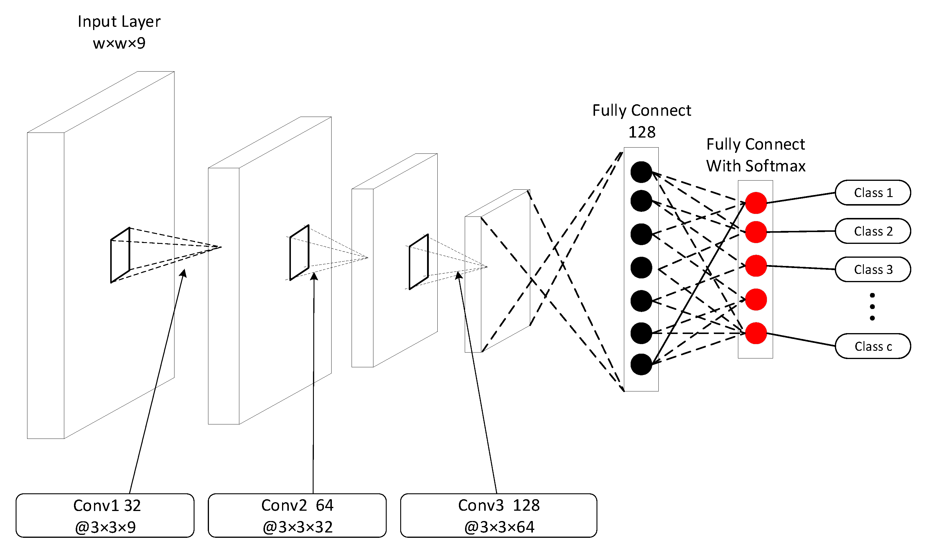
2.3.2. Network Architecture

Neural networks have achieved great success in computer vision applications. Compared with manual feature extraction, DNN can learn the hidden information of the data actively. AlexNet [22] has demonstrated to have excellent performance compared to traditional models in image classification. After that, more powerful DNN algorithms have been proposed, such as VGG [23], ResNet [24], GoogLeNet [25] and DenseNet [26], etc., achieving a superior performance in almost all vision applications.

The SCNN model is based on a basic deep CNN [27], which is used to extract features in classification. This model is easy to train and performs well on PolSAR image classification. As shown in Figure 2, the architecture of the SCNN model consists of three convolution layers, two fully connected layers, and a softmax classifier. Each convolution layer is followed by a max-pooling layer ignoring small variation in the training data [28], with a pooling size $2\times 2$ and a stride of 2. We use switchable normalization (SN) [29] as the normalization method which combines and assigns weights to batch normalization, layer normalization, and instance normalization.

The loss function of the proposed SCNN model consists of two terms as shown in Equation (4), with the classification loss $L_{classification}$ and the similarity loss $L_{similarity}$.

$$L=L_{classification}+L_{similarity}$$

(4)

where cross entropy is used to calculate $L_{classification}$ as shown in Equation (5).

$$L_{classification}=-\sum _{k=1}^c{y}_{k}log{\widehat{y}}_k$$

(5)

where c is the number of classes, $y_k$ and ${\widehat{y}}_k$ are the actual and predicted probability of the sample in the k-th class, respectively.

A similarity loss is introduced in the SCNN model to strengthen extracted features from those pixels in the same class with a higher similarity. In the subsequent label propagation, we can assign pseudo labels to unlabeled data according to the similarity between features. The similarity loss $L_{similarity}$ in Equation (4) is defined by the cosine distance, shown in Equation (6):

$$L_{similarity}=\frac{1}{n^2}\sum _{i=1}^n\sum _{j=1}^{n}cosine(fea{t}_i,fea{t}_j)·F_{ij}$$

(6)

$$F_{ij}=\left\{\begin{array}{cc}\hfill -1& ,class\left(fea{t}_i\right)=class\left(fea{t}_j\right)\hfill \\ \hfill 1& ,else\hfill \end{array}\right.$$

(7)

where, n represents the number of labeled samples, $fea{t}_i$ represents the feature of the i-th sample extracted by the SCNN model. If $fea{t}_i$ and $fea{t}_j$ belong to the same category, $F_{ij}$ is −1, otherwise $F_{ij}$ is 1.

Like in [14], the cosine distance is defined in Equation (8). Larger value means the two samples are more similar.

$$cosine\left(fea{t}_i,fea{t}_j\right)=\frac{fea{t}_i·fea{t}_j}{∥fea{t}_i∥∥fea{t}_j∥}$$

(8)

2.4. Label Propagation

Label propagation is defined as propagating the labels from labeled samples to unlabeled samples, i.e., assign pseudo labels to unlabeled samples. In FS-SCNN, features are extracted from labeled and unlabeled samples using SCNN. The features from the fully connected layer of SCNN are used. By measuring the similarity between the features, we assign pseudo labels to unlabeled samples in U. The accuracy of the label propagation is improved using the following two steps to give labels to unlabeled samples. In step 1, the similarity between unlabeled samples and labeled samples is measured using cosine distance. Only if certain conditions are met, we go to step 2 to confirm whether to assign pseudo labels to unlabeled samples. In step 2, the similarity between labeled and unlabeled superpixels is used to help label propagation, considering each labeled (unlabeled) sample is selected from its corresponding superpixels. If two superpixels are similar, then the samples extracted from the two superpixels are regarded as similar.

Step 1: Assign pseudo labels based on the maximum similarity

For any unlabeled sample $u_k$ in U, the average cosine distance between $u_k$ and pixels in labeled samples $L=\left[L_1,L_2,\dots ,L_t,\dots ,L_c\right]$ is calculated using Equation (8), i.e., $\left[S_{k1},S_{k2},\dots ,S_{kt},\dots ,S_{kc}\right]$. Then the maximum similarity $S_{kt}$ and the labeled sample set $L_t$ are obtained. Next, compute the average similarity ${\overline{S}}_t$ between features extracted from the labeled sample set $L_t$. If $S_{kt}>{\overline{S}}_t$, then go to step 2. Otherwise, no pseudo label is assigned to the unlabeled sample $u_k$.

Step 2: Confirm the pseudo label based on the superpixels

The Wishart distance is widely used for measuring the distance between pixels based on the complex Wishart distribution of PolSAR images. In this paper, we adopt a revised Wishart distance named SRW [30] to calculate the similarity between superpixels, defined as in Equation (9):

$$D_{SRW}\left(i,j\right)=\frac{1}{2}\left(tr\left({\overline{T}}_i^{-1}{\overline{T}}_j\right)+tr\left({\overline{T}}_j^{-1}{\overline{T}}_i\right)\right)-3$$

(9)

where, ${\overline{T}}_i$ and ${\overline{T}}_j$ represents the covariance matrix of cluster centers of the i-th and j-th superpixels, respectively. The smaller the $D_{SRW}$, the more similar the two superpixels are.

With Equation (9), the average SRW distance $D_{SRWul}$ between unlabeled superpixels $su{p}_u$ and labeled superpixels $Su{p}_{l_t}=\left\{su{p}_1,su{p}_2,\cdots ,su{p}_z\right\}$ is calculated. The superpixels in the set $Su{p}_{l_t}$ have the same label t. Then the average Wishart distance ${\overline{S}}_{SR{W}_t}$ between the labeled superpixels in set $Su{p}_{l_t}$ is calculated. If $D_{SRWul}<{\overline{S}}_{SR{W}_t}$, then assign label t to the unlabeled sample $u_k$ and add $u_k$ to the labeled sample set L. Otherwise $u_k$ is still unlabeled.

2.5. Procedure of the FS-SCNN Algorithm

The FS-SCNN algorithm is presented in Algorithm 1.

Algorithm 1 FS-SCNN

Input: PolSAR image, the initialization iteration $t=0$, the number of iterations $tmax$ Output: Trained classification model (1) Use the Fs algorithm to produce superpixels and undetermined pixels. (Section 2.1) (2) Construct labeled and unlabeled sample set (L and U) using superpixels and undetermined pixels. (Section 2.2) (3) While $t<tmax$ or unlabeled samples set U is not empty:      Train the SCNN model using labeled samples L. (Section 2.3)      Use the trained SCNN model to learn the features from samples in L and U. (Section 2.3)      Assign pseudo labels to unlabeled samples using a two-step strategy. Add samples with pseudo labels to L and remove them from U. (Section 2.4) (4) End while

3. Experiments

3.1. Data Sets and Experiments Setting

The effectiveness of FS-SCNN is demonstrated on three widely tested PolSAR dataset. The first data set is San Francisco (San) of size $1300\times 1300$ pixels, which is the four-look L-band PolSAR image. The Pauli RGB image is shown in Figure 3a, and the ground truth (GT) map is shown in Figure 3b. It contains five categories, which are LD urban, water, veg, HD urban and Developed. The color code of each category is shown in Figure 3c.

The second PolSAR image, Flevoland (Fle) acquired by the AIRSAR airborne platform in 1989, is shown in Figure 4. Fle is a four-look L-band image of size $300\times 270$ pixels with the ground truth map in Figure 4b and color code in Figure 4c. Pixels in the image are classified into six categories: bare soil, potatoes, beet, forest, wheat, and peas.

The third PolSAR data named Flevoland1991 (Fle1991) is the L-band image of size $430\times 280$ pixels. There are seven categories in Flevoland1991: barley, wheat, rape seed, grass, beet, potatoes and flax, respectively. The Pauli RGB image, the GT map and the color code are shown in Figure 5.

To demonstrate the performance of the FS-SCNN method, we compare FS-SCNN with four state-of-the-art PolSAR classification methods, RV-CNN [27], CV-CNN [21], LS-QCNN [31] and STS [10]. In the process of fuzzy superpixels-based sample sets selection, the sliding window and the step are set to 8 × 8 and 1, respectively. We use adaptive moment estimation (Adam) [32] to optimize the proposed SCNN model. The learning rate is 0.001 and the number of epochs is 100.

The classification accuracy of each category and overall accuracy (OA) are adopted to verify the performance of the methods. OA is the percentage of correctly classified pixels among all the pixels, which is not related to the category of pixels.

3.2. Experiments on San Francisco Data

Fifty pixels are selected randomly from each category as initially labeled pixels. The proposed algorithm first extends the number of labeled pixels based on fuzzy superpixels and selects labeled and unlabeled samples based on the extended labeled pixels for the proposed SCNN network (see Section 2.2). Then the trained SCNN (see Section 2.3) is used to propagate labels, i.e., assign pseudo labels to unlabeled samples (see Section 2.4).

Table 1. The numbers of increased labeled pixels on San Francisco data.

	Num. of the Initially Labeled Pixels Pixels	Num. of the Extended Labeled Pixels	Num. of Labeled Pixels by Label Propagation (Iteration 1)	Num. of Labeled Pixels by Label Propagation (Iteration 2)	Num. of Labeled Pixels by Label Propagation (Iteration 3)
Water	50	6414	12,079	648	1375
Veg	50	6909	14,348	12,157	1175
LD Urban	50	4294	15,223	5857	5220
HD Urban	50	4970	14,557	20,047	12,232
Developed	50	4294	12,786	5007	2430
All	250	26,881	68,993	43,716	22,432
OA	0.8483	0.8813	0.9607	0.9382	0.9267

shows the numbers of increased labeled pixels for San Francisco. The best result for OA is in bold. From Table 1 we can see that both the extension of initially labeled pixels based on fuzzy superpixels and label propagation based on SCNN increase the number of labeled pixels. A large number of pseudo labeled pixels can be obtained by label propagation. As the number of iterations of SCNN increases, more pseudo labeled pixels are obtained. However, it is not that the more pseudo labeled pixels, the higher the accuracy, due to some false labels in the pseudo labeled pixels. For San Francisco, the classification accuracy reaches the maximum value when the number of iteration of SCNN is 1.

We select the number of superpixels according to that in [15] where better performance is obtained when the number of superpixels is 3000 for San Francisco. In our algorithm, the number of superpixels is doubled to reduce the generation of mixed superpixels. The experiments shown in Figure 6 demonstrate the performance of label propagation explained in Section 2.4, with two steps to assign pseudo labels to unlabeled samples. “Only using cosine distance” means only use step 1 to propagate labels, and “using both cosine distance and Wishart distance” represents using two steps (step 1 and step 2) to propagate labels. Figure 6a shows the accuracy of pseudo labels in label propagation only using cosine distance and using both cosine distance and Wishart distance. Figure 6b shows the accuracy of the classification using pseudo labels. From the figures, we can see that:

(1) In the case where both Wishart distance and cosine distance are used (Figure 6a), the accuracy of pseudo labels is the highest at the first iteration in Algorithm 1, which is about 97%. Then the accuracy of pseudo labels slowly decreases with the number of iterations, and finally stabilizes at around 94% on the fifth iteration. When only cosine distance is used, the accuracy of pseudo labels is about 95% in the first three iterations, and dropped and stabilized at around 92% after the fourth iteration. The accuracy of pseudo labels is higher when using both cosine distance and Wishart distance.

(2) The accuracy of classification starts from 88% using only the original labeled samples (i.e, the accuracy without label propagation), and reaches the maximum 96% at the first iteration. Then the classification accuracy of pseudo labels gradually decreases, finally stabilizes at around 92%. Therefore, for the San Francisco data, we set $tmax$ to 1. In Figure 6b, the results using only the cosine distance indicate that the accuracy of classification on San Francisco is increased from 88% to 94% in the first three iterations and then slowly decreased. Comparing the two curves in Figure 6b, the classification results are more accurate with fewer iterations when using both cosine distance and Wishart distance.

To demonstrate the effectiveness of the similarity loss term in the loss function, as shown in Equation (6), we compare the proposed SCNN with a standard CNN. The loss function of SCNN consists of the classification loss and the similarity loss, shown in Equation (4). The loss function of CNN only uses the classification loss in Equation (4). Firstly, SCNN and CNN are used to learn features from samples, respectively. Then, the average similarity is calculated between the features belonging to the same category. The similarity between samples belonging to the same category is calculated using Equation (6), as shown in Figure 7, showing that the features extracted from samples belonging to the same category by SCNN are significantly more similar than those by CNN.

The classification accuracy of FS-SCNN and other compared methods are shown in

Table 2. Classification accuracy comparisons on San Francisco.

	RV-CNN	CV-CNN	LS-QCNN	STS	FS-SCNN
Water	0.9791	0.9978	0.9994	0.9984	0.9962
Veg	0.8830	0.9304	0.9647	0.8955	0.9287
LD Urban	0.6447	0.9042	0.7261	0.6300	0.9074
HD Urban	0.8624	0.8507	0.8395	0.8803	0.9275
Developed	0.8835	0.6946	0.8540	0.7745	0.9377
OA	0.9084	0.9350	0.9398	0.9140	0.9607

. Values in bold indicate the best result of each category and OA. FS-SCNN achieves the highest accuracies on three categories, with an accuracy exceeding 90% in all categories. Besides, FS-SCNN outperforms the other methods in terms of OA, i.e 96.07%, which is 5.23%, 2.57%, 2.09%, and 4.67% higher than RV-CNN, CV-CNN, LS-QCNN and STS, respectively.

Figure 8 shows the visual displays of the classification results from where a selected enlarged region is shown in Figure 9. The grey pixels in the two figures are misclassified pixels. From Figure 8 and Figure 9, we can see that the classification accuracies of RV-CNN on the low-density area (red area) are very poor. Almost half of the pixels are misclassified. There are also many misclassified pixels in developed (yellow area) and high-density urban (purple area). CV-CNN has many errors in developed. The LS-QCNN method performs well on water and vegetation, and poorly on low-density urban. The STS method has a higher performance only on water. The FS-SCNN proposed in this paper performs well in all categories.

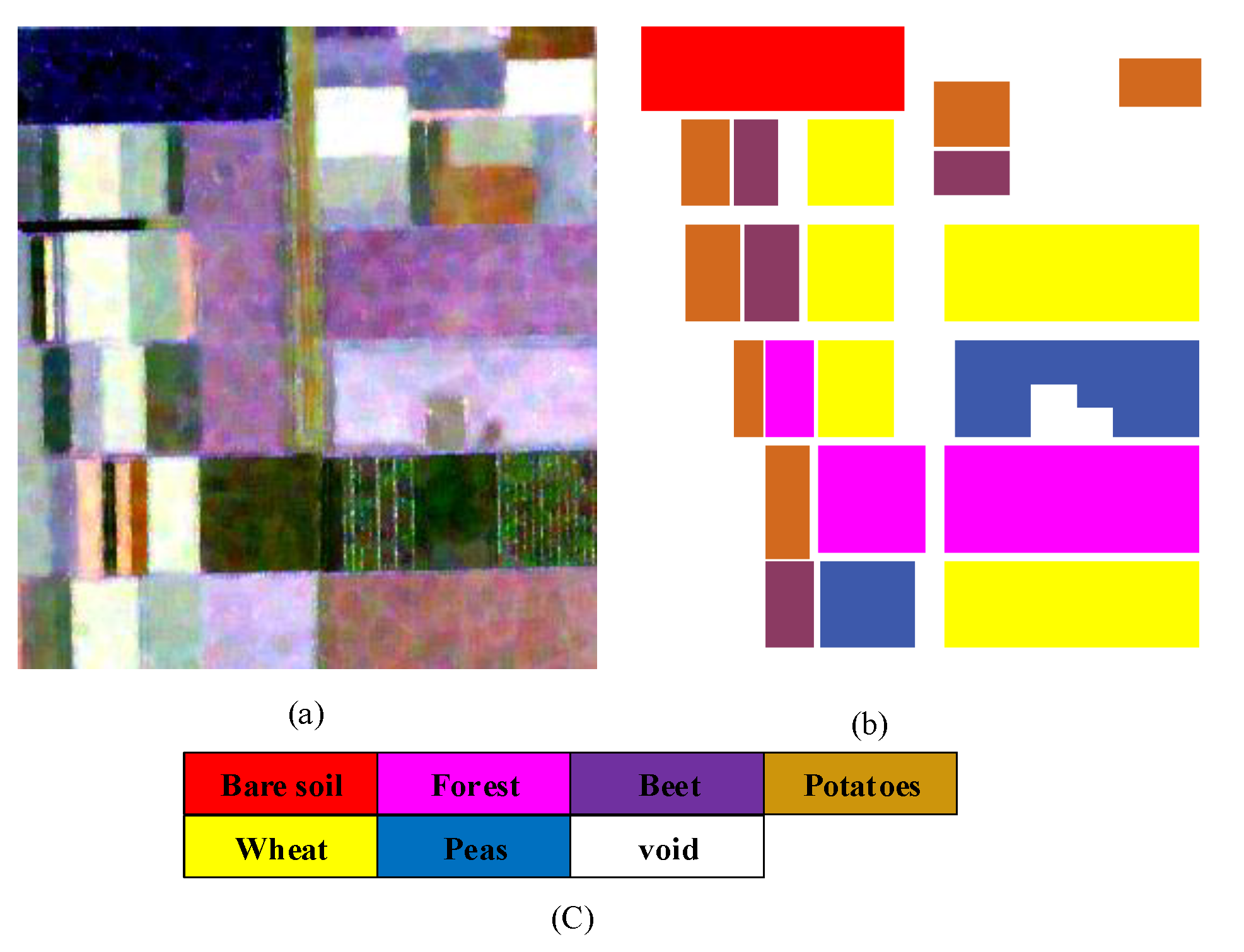
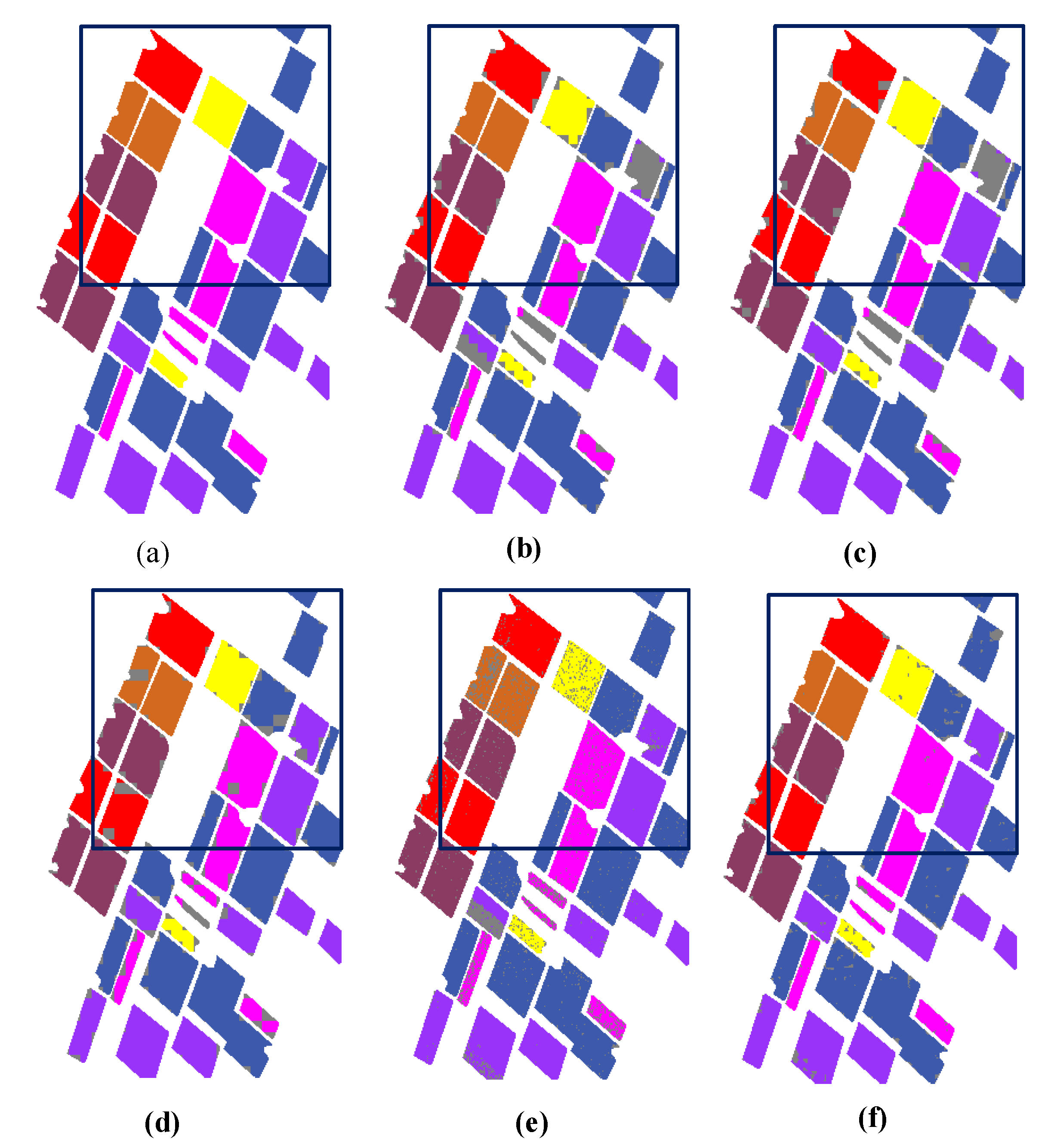
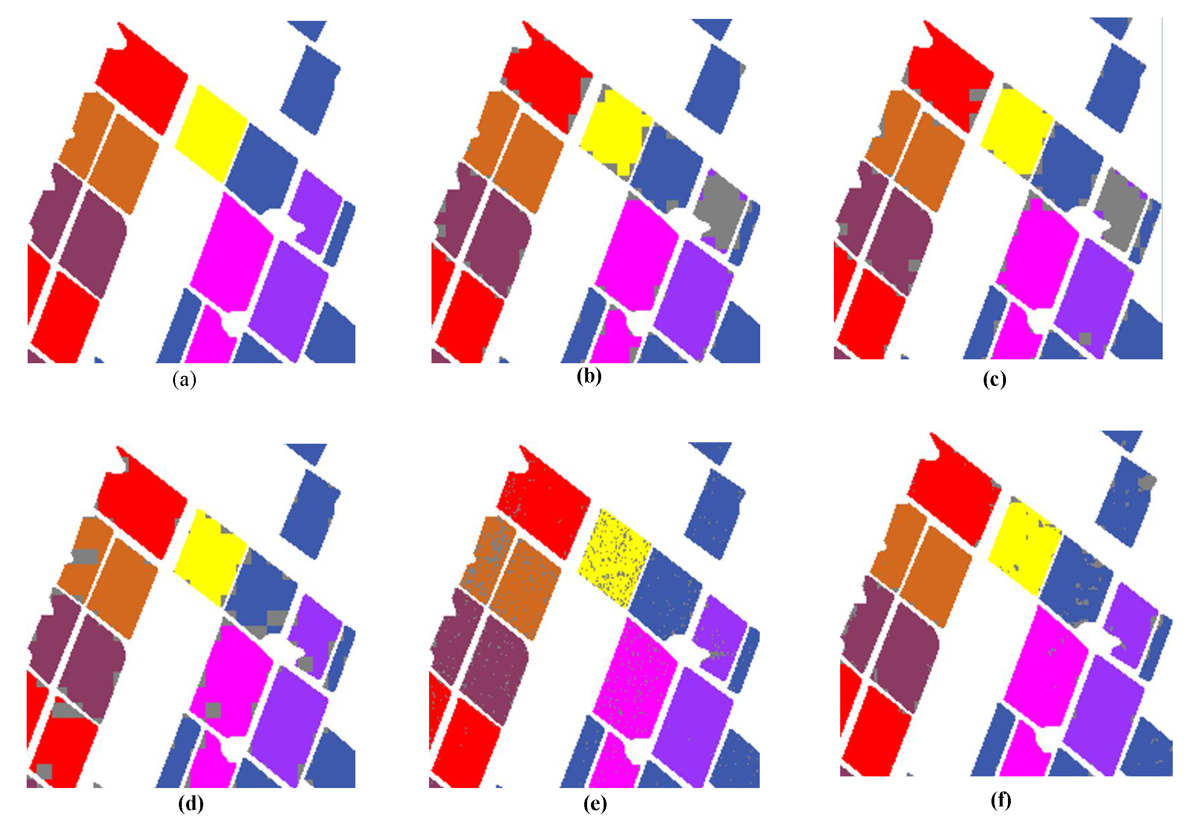
3.3. Experiments on Flevoland Data

In the Flevoland data, the number of generated superpixel is 1000. Ten pixels in each category are selected randomly as the labeled pixels.

Figure 10a,b shows the accuracy of the pseudo labels during the label propagation and the classification performance after each iteration in Algorithm 1. The accuracy of the label propagation is stable between 92% and 94%. The classification accuracy starts from 91% using only the original labeled samples, and reaches 94% after two iterations, then begins to decrease slowly. So for Flevoland Data, we set $tmax$ to 2.

Figure 11 shows the OA of each method showing FS-SCNN still performs better on Flevoland data. Compared with CV-CNN, RV-CNN, LS-QCNN and STS algorithms, the OA of FS-SCNN on the Flevoland data are improved by 4.80%, 3.13%, 1.61% and 0.58%, respectively.

Figure 12a shows the GT for Flevoland. Figure 12b–f shows classification maps obtained by different methods which performs poorly on some of the categories or have many misclassified pixels. FS-SCNN performs well in all categories.

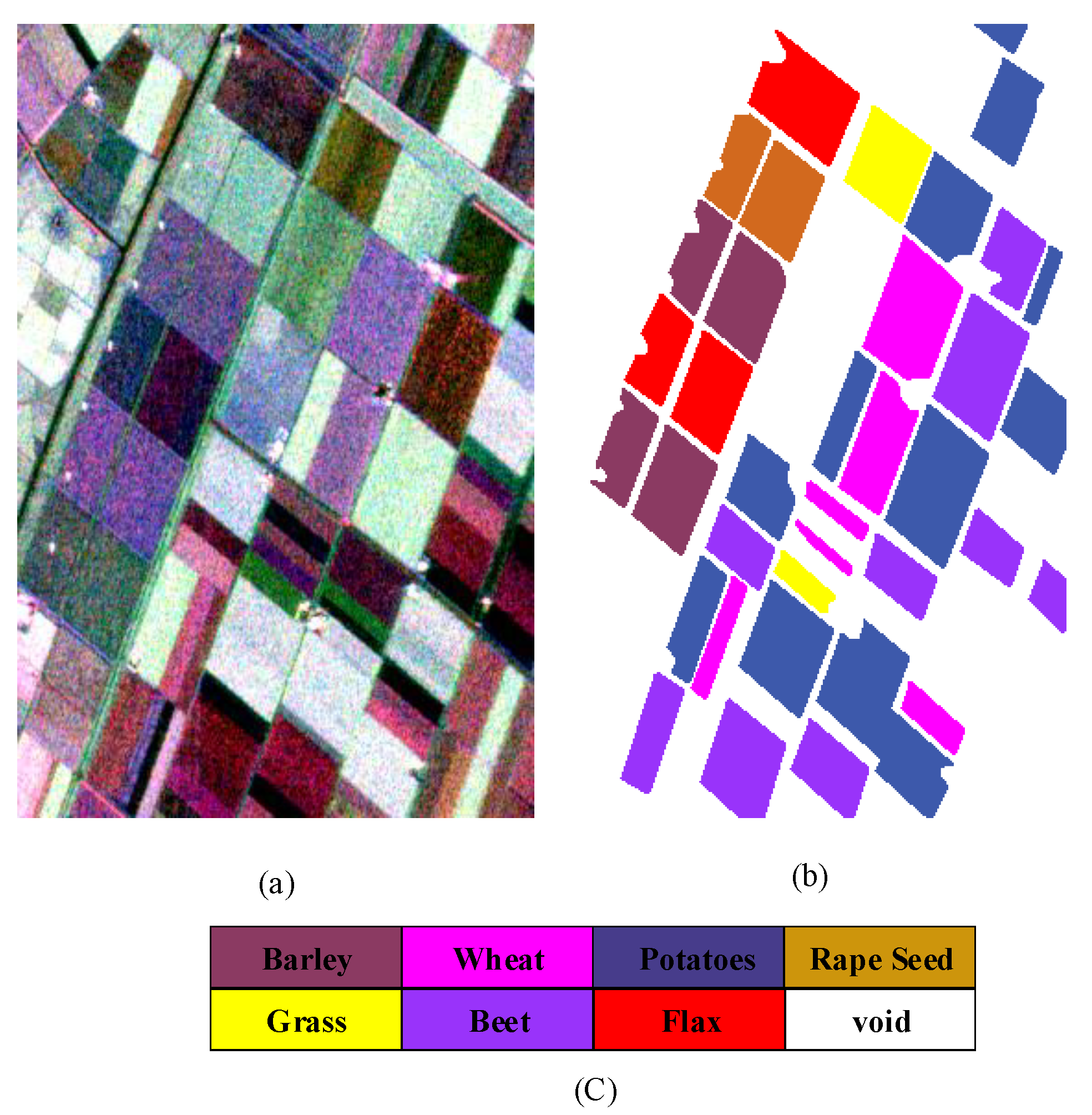
3.4. Experiments on Flevoland1991 Data

The expected number of superpixels is set to 1000 for Flevoland1991 data. Five labeled pixels are selected randomly from each category.

Figure 13 shows the accuracy of the pseudo label and the accuracy of classification after each iteration. For the same reasons as above, we set $tmax$ to 2.

To demonstrate the superiority of the Fs algorithm, we compared Fs with two other superpixel algorithms on the Flevoland1991 dataset. These two algorithms are SLIC [33] and LSC [34]. The classification accuracy using different superpixel algorithms is shown in Figure 14. The accuracy of Fs algorithm exceeds both the other two superpixels algorithms at the first iteration and continues to reach the highest after the second iteration. Therefore, using Fs algorithm is better than the other two algorithms across all the iterations of label propagation in Algorithm 1.

The classification accuracy of each category and OA are shown in

Table 3. Classification accuracy comparisons on Flevoland1991.

	RV-CNN	CV-CNN	LS-QCNN	STS	FS-SCNN
Flax	0.9460	0.9479	0.9268	0.9665	0.9740
Rape Seed	0.9886	0.9466	0.9167	0.8157	0.9893
Barely	0.9545	0.9424	0.9489	0.9633	0.9691
Grass	0.8702	0.9376	0.9276	0.8385	0.9398
Wheat	0.8361	0.8429	0.8450	0.8702	0.9737
Potatoes	0.9668	0.9542	0.9473	0.9753	0.9563
Beet	0.8474	0.8745	0.9447	0.9283	0.9758
OA	0.9177	0.9207	0.9296	0.9346	0.9672

. The best result for each category and OA is in bold. It can be seen that FS-SCNN performs well in most categories and achieves the highest accuracy in six out of seven categories. OA of FS-SCNN reaches 96.72%. Compared with CV-CNN, RV-CNN, LS-QCNN and STS, it is improved by 4.95%, 4.65%, 3.76% and 3.26%, respectively.

The visual display of classification is shown in Figure 15. The enlarged regions are shown in Figure 16. We can see that the performance of the two algorithms RV-CNN and CV-CNN is poor on beet and wheat, and LS-QCNN has many misclassified pixels on wheat. The classification performance of STS performs poorly on grass and rape seed. FS-SCNN has few misclassified pixels in potatoes and performs well on other categories.

4. Discussion

The FS-SCNN method presents excellent advantages in PolSAR image classification with limited labeled data according to the experimental results. The reasons include the following: First, the concept of fuzzy superpixels is adopted to suppress the impact of mixed superpixels on classification accuracy. Second, the similarity-constrained term is considered by SCNN, which strengthens the similarity between features extracted from the same category. Third, two steps are adopted to assign labels to unlabeled samples using different distance evaluation criteria to measure the similarity.

The following points are worth discussing.

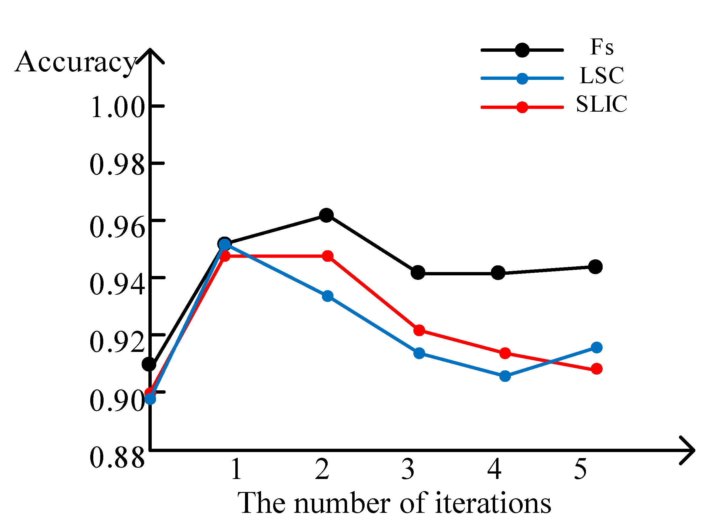
• The superiority of fuzzy superpixels. Superpixels generation techniques can be used to extend the labeled sample. That is, given the label of any pixel in a superpixel, all pixels in the superpixel will be labeled. However, there are mixed superpixels in practical applications. Figure 14 indicates that Fs is better than other superpixels algorithms. In the preprocessing step, the extended labeled samples by superpixels should be as accurate as possible. Fs divides an image into superpixels and undetermined pixels, which strengthens the correctness of the extended labeled samples.
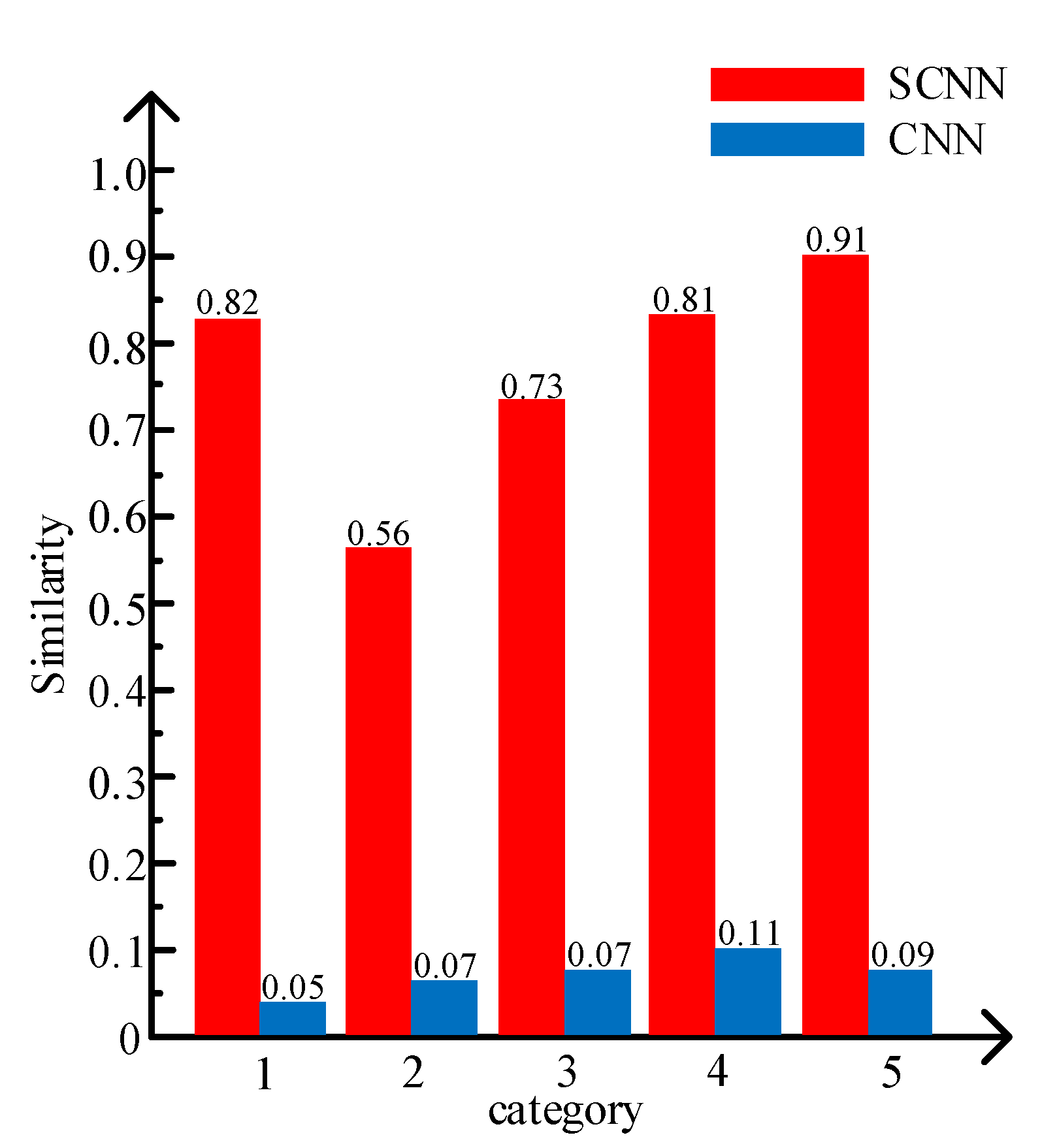
• The validity of the similarity-constrained term. Figure 7 shows that the features extracted from samples with the same category by SCNN are more similar than those extracted by CNN due to the similarity-constrained term, which strengthens the similarity between features of the same category.
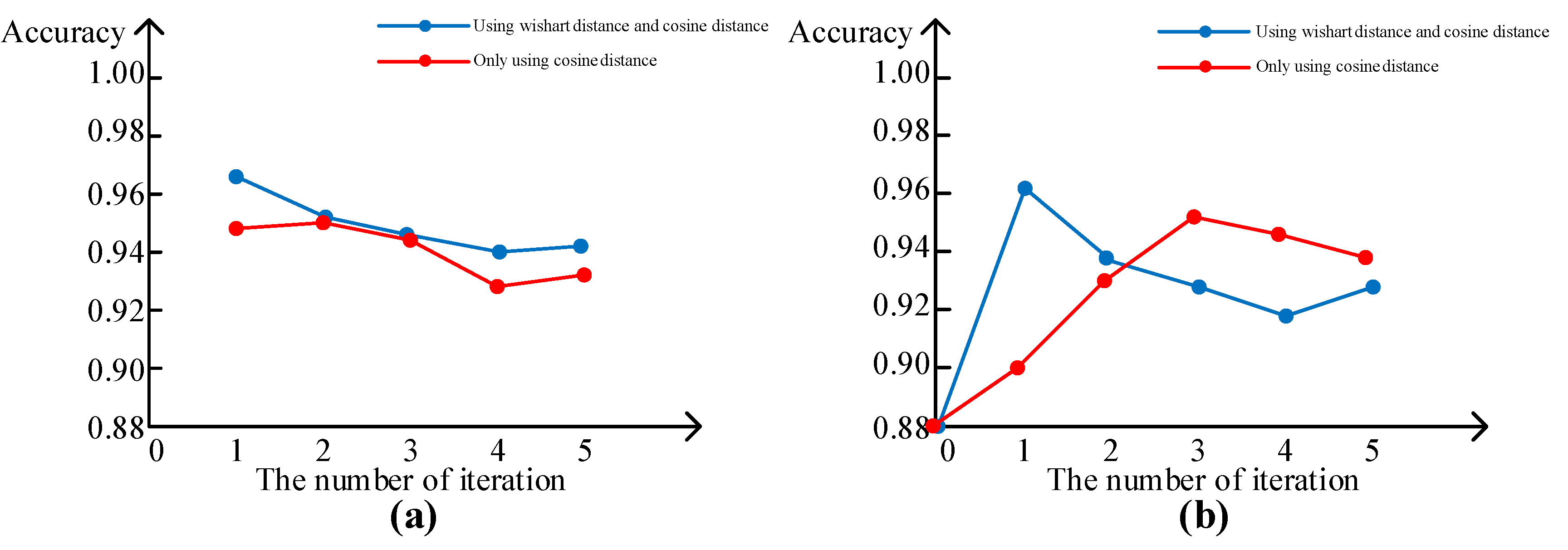
• The different distance measurement criteria. There are two steps in the label propagation. Step 1, cosine distance is used to assign pseudo labels to unlabeled samples. Step 2, Wishart distance is adopted to confirm the pseudo labels obtained in Step 1. Figure 6 shows that using both cosine distance and Wishart distance contributes to better PolSAR image classification.
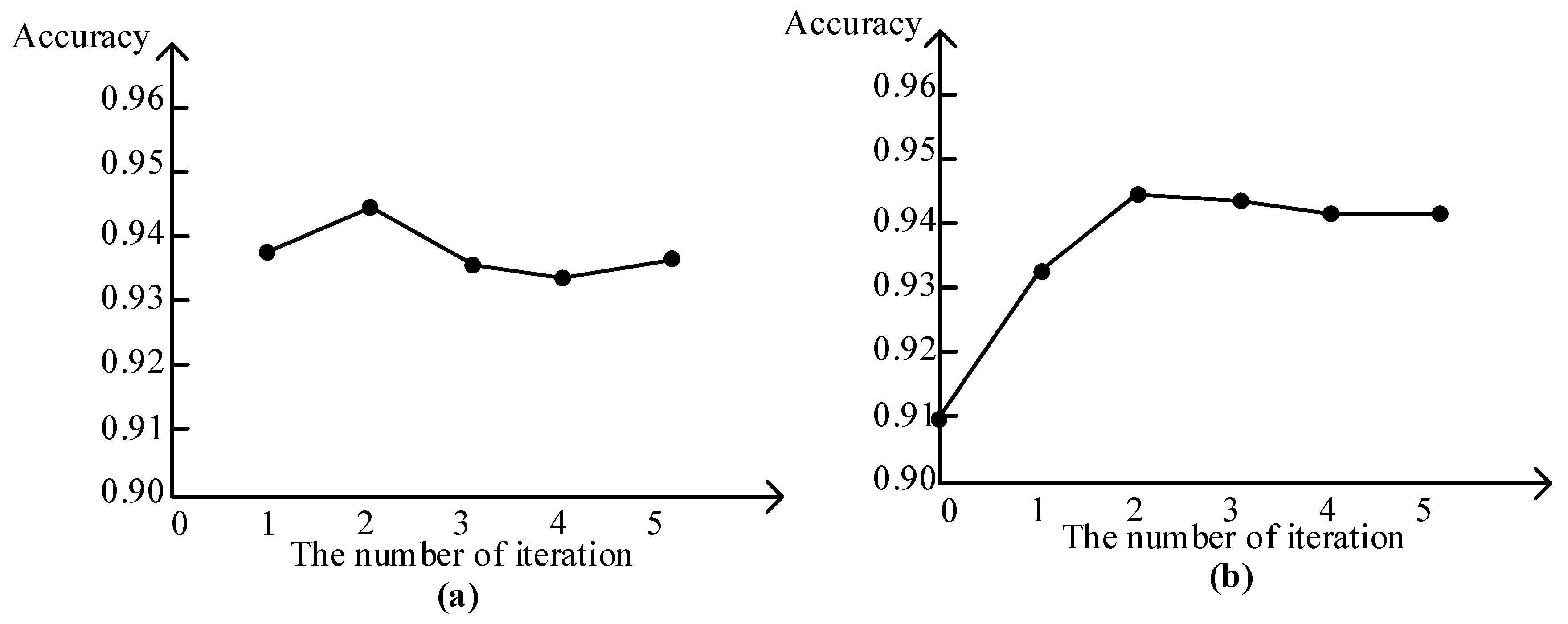
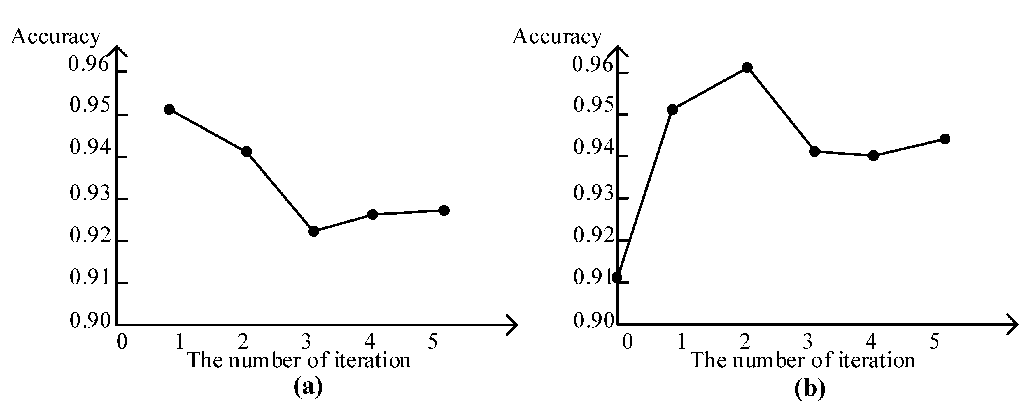
• The role of label propagation. As the iterations increases of Algorithm 1, the accuracy of the pseudo labels slowly decreases and then stabilizes. With an increased number of pseudo labels, the classification accuracy increases first, then decreases slowly after reaching the highest value, and finally stabilizes near a certain value. It demonstrates that the added of pseudo labels can improve the classification accuracy of the network model.
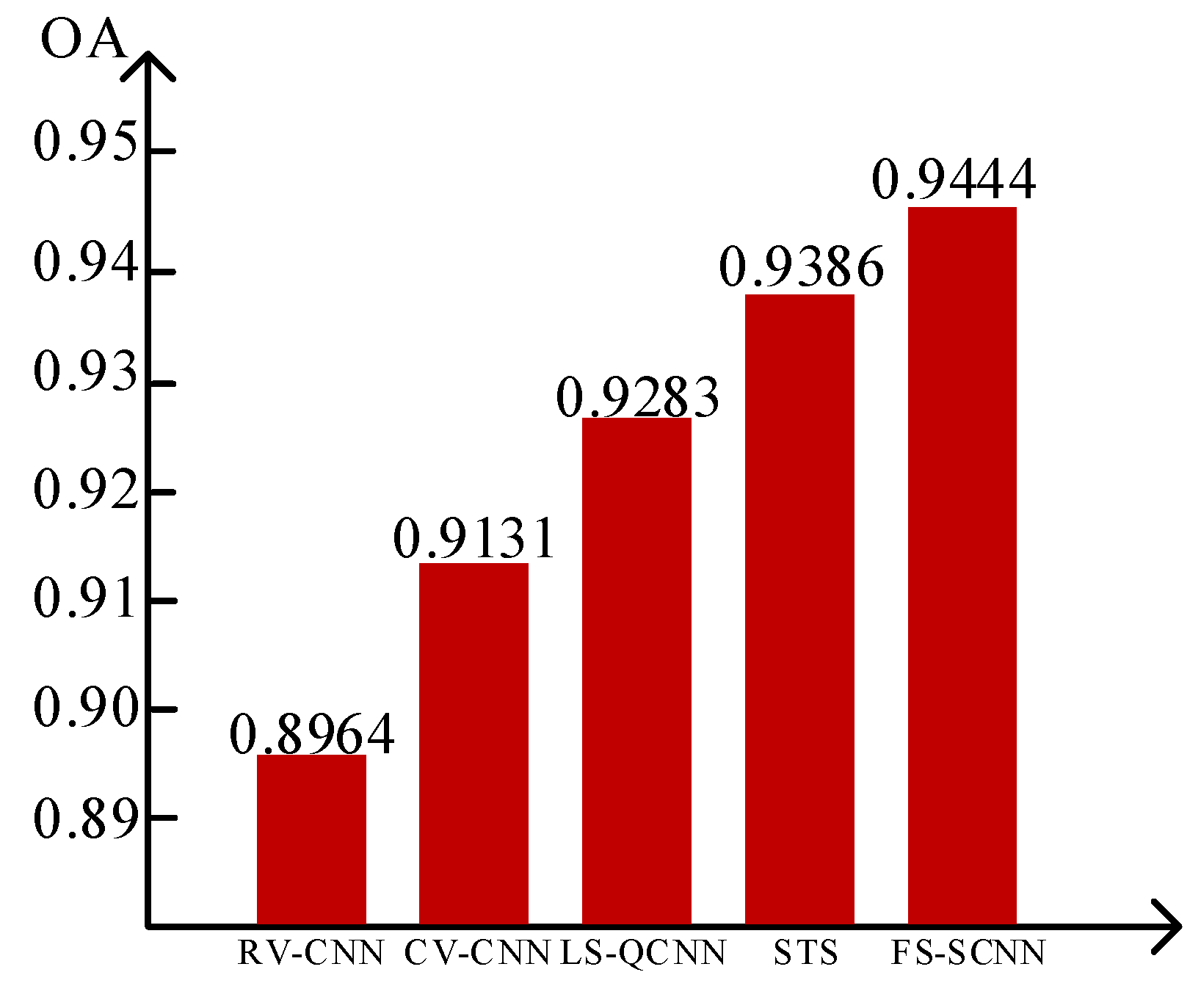
• The parameter S.

  Table 4. OA under different values of parameter S.

  	S	0.1	0.2	0.3	0.4	0.5
  Data
  San Francisco		0.9607	0.9397	0.9304	0.9275	0.9312
  Flevoland		0.9032	0.9133	0.9390	0.9385	0.9444
  Flevoland1991		0.6929	0.7352	0.9672	0.9473	0.9239

  shows that the accuracy changes with parameter S, from which we can see that the value of S corresponding to the highest accuracy is different for different data. The best result for each dataset is in bold. In our experiments, to achieve better classification performance, we set S to 0.1, 0.5 and 0.3 for San Francisco, Flevoland and Flevoland1991 data, respectively.

5. Conclusions

A novel fuzzy superpixels based semi-supervised similarity-constrained CNN for the PolSAR image classification method is proposed in this paper. The proposed algorithm has several attractive features which contribute to its classification performance. Instead of using a traditional superpixels algorithm, a fuzzy superpixels algorithm Fs is used in FS-SCNN to divide the PolSAR image into superpixels and undetermined pixels, so that the generation of mixed superpixels is suppressed. The similarity-constrained CNN (SCNN) model is proposed using a similarity-constrained term in the loss function to strengthen that the extracted features from the same category are as similar as possible. Then, we can use the similarity to propagate labels to unlabeled samples. Moreover, two distance measures, cosine distance and Wishart distance, are used to achieve a higher accuracy ratio for label propagation. With these specific mechanisms integrated, FS-SCNN is reported to outperform four existing CNN algorithms in terms of classification performance on three widely used PolSAR images.

In terms of future work, we plan to improve the performance of semi-supervised CNN by introducing ensemble learning techniques, as considering different models in the knowledge base under different conditions could obtain a superior prediction [35,36].

References

1. Deng, L.; Yan, Y.; Sun, C. Use of sub-aperture decomposition for supervised PolSAR classification in urban area. Remote Sens. 2015, 7, 1380–1396. [Google Scholar] [CrossRef] [Green Version]
2. Ji, Y.; Sumantyo, S.; Tetuko, J.; Chua, M.Y.; Waqar, M.M. Earthquake/tsunami damage assessment for urban areas using post-event PolSAR data. Remote Sens. 2018, 10, 1088. [Google Scholar] [CrossRef] [Green Version]
3. Mascolo, L.; Lopez-Sanchez, J.M.; Vicente-Guijalba, F.; Nunziata, F.; Migliaccio, M.; Mazzarella, G. A complete procedure for crop phenology estimation with PolSAR data based on the complex Wishart classifier. IEEE Trans. Geosci. Remote Sens. 2016, 54, 6505–6515. [Google Scholar] [CrossRef] [Green Version]
4. Hajnsek, I.; Jagdhuber, T.; Schon, H.; Papathanassiou, K.P. Potential of estimating soil moisture under vegetation cover by means of PolSAR. IEEE Trans. Geosci. Remote Sens. 2009, 47, 442–454. [Google Scholar] [CrossRef] [Green Version]
5. Safari, K.; Prasad, S.; Labate, D. A Multiscale Deep Learning Approach for High-Resolution Hyperspectral Image Classification. IEEE Geosci. Remote Sens. Lett. 2020. [Google Scholar] [CrossRef]
6. Wu, X.; Sahoo, D.; Hoi, S.C. Recent advances in deep learning for object detection. Neurocomputing 2020, 396, 39–64. [Google Scholar] [CrossRef] [Green Version]
7. Wang, R.; Wang, Y. Classification of PolSAR Image Using Neural Nonlocal Stacked Sparse Autoencoders with Virtual Adversarial Regularization. Remote Sens. 2019, 11, 1038. [Google Scholar] [CrossRef] [Green Version]
8. Chen, W.; Gou, S.; Wang, X.; Li, X.; Jiao, L. Classification of PolSAR images using multilayer autoencoders and a self-paced learning approach. Remote Sens. 2018, 10, 110. [Google Scholar] [CrossRef] [Green Version]
9. Bi, H.; Sun, J.; Xu, Z. A graph-based semisupervised deep learning model for PolSAR image classification. IEEE Trans. Geosci. Remote Sens. 2018, 57, 2116–2132. [Google Scholar] [CrossRef]
10. Li, Y.; Xing, R.; Jiao, L.; Chen, Y.; Chai, Y.; Marturi, N.; Shang, R. Semi-Supervised PolSAR Image Classification Based on Self-Training and Superpixels. Remote Sens. 2019, 11, 1933. [Google Scholar] [CrossRef] [Green Version]
11. Xie, W.; Ma, G.; Zhao, F.; Liu, H.; Zhang, L. PolSAR image classification via a novel semi-supervised recurrent complex-valued convolution neural network. Neurocomputing 2020, 388, 255–268. [Google Scholar] [CrossRef]
12. Sun, Q.; Li, X.; Li, L.; Liu, X.; Liu, F.; Jiao, L. Semi-Supervised Complex-Valued GAN for Polarimetric SAR Image Classification. In Proceedings of the IGARSS 2019-2019 IEEE International Geoscience and Remote Sensing Symposium, Yokohama, Japan, 28 July–2 August 2019; pp. 3245–3248. [Google Scholar]
13. Hou, B.; Guan, J.; Wu, Q.; Jiao, L. Semisupervised Classification of PolSAR Image Incorporating Labels’ Semantic Priors. IEEE Geosci. Remote Sens. Lett. 2019, 1–5. [Google Scholar] [CrossRef]
14. Geng, J.; Ma, X.; Fan, J.; Wang, H. Semisupervised classification of polarimetric SAR image via superpixel restrained deep neural network. IEEE Geosci. Remote Sens. Lett. 2017, 15, 122–126. [Google Scholar] [CrossRef]
15. Guo, Y.; Jiao, L.; Wang, S.; Wang, S.; Liu, F.; Hua, W. Fuzzy superpixels for polarimetric SAR images classification. IEEE Trans. Fuzzy Syst. 2018, 26, 2846–2860. [Google Scholar] [CrossRef]
16. Oliver, A.; Odena, A.; Raffel, C.A.; Cubuk, E.D.; Goodfellow, I. Realistic evaluation of deep semi-supervised learning algorithms. In Proceedings of the Advances in Neural Information Processing Systems, Vancouver, BC, Canada, 3–8 December 2018; pp. 3235–3246. [Google Scholar]
17. Zhu, X.X.; Tuia, D.; Mou, L.; Xia, G.S.; Zhang, L.; Xu, F.; Fraundorfer, F. Deep learning in remote sensing: A comprehensive review and list of resources. IEEE Geosci. Remote Sens. Mag. 2017, 5, 8–36. [Google Scholar] [CrossRef] [Green Version]
18. Haeusser, P.; Mordvintsev, A.; Cremers, D. Learning by Association–A Versatile Semi-Supervised Training Method for Neural Networks. In Proceedings of the IEEE Conference on Computer Vision and Pattern Recognition, Honolulu, HI, USA, 21–26 July 2017; pp. 89–98. [Google Scholar]
19. Ren, X.; Malik, J. Learning a classification model for segmentation. In Proceedings of the Ninth IEEE International Conference on Computer Vision, Nice, France, 13–16 October 2003; p. 10. [Google Scholar]
20. Wang, W.; Xiang, D.; Ban, Y.; Zhang, J.; Wan, J. Superpixel-based segmentation of polarimetric SAR images through two-stage merging. Remote Sens. 2019, 11, 402. [Google Scholar] [CrossRef] [Green Version]
21. Zhang, Z.; Wang, H.; Xu, F.; Jin, Y.Q. Complex-valued convolutional neural network and its application in polarimetric SAR image classification. IEEE Trans. Geosci. Remote Sens. 2017, 55, 7177–7188. [Google Scholar] [CrossRef]
22. Krizhevsky, A.; Sutskever, I.; Hinton, G.E. Imagenet classification with deep convolutional neural networks. In Proceedings of the Advances in Neural Information Processing Systems, Lake Tahoe, NV, USA, 3–6 December 2012; pp. 1097–1105. [Google Scholar]
23. Simonyan, K.; Zisserman, A. Very deep convolutional networks for large-scale image recognition. arXiv 2014, arXiv:1409.1556. [Google Scholar]
24. He, K.; Zhang, X.; Ren, S.; Sun, J. Deep residual learning for image recognition. In Proceedings of the IEEE Conference on Computer Vision and Pattern Recognition, Las Vegas, NV, USA, 27–30 June 2016; pp. 770–778. [Google Scholar]
25. Szegedy, C.; Liu, W.; Jia, Y.; Sermanet, P.; Reed, S.; Anguelov, D.; Erhan, D.; Vanhoucke, V.; Rabinovich, A. Going deeper with convolutions. In Proceedings of the IEEE Conference on Computer Vision and Pattern Recognition, Boston, MA, USA, 7–12 June 2015; pp. 1–9. [Google Scholar]
26. Huang, G.; Liu, Z.; Van Der Maaten, L.; Weinberger, K.Q. Densely connected convolutional networks. In Proceedings of the IEEE Conference on Computer Vision and Pattern Recognition, Honolulu, HI, USA, 21–26 July 2017; pp. 4700–4708. [Google Scholar]
27. Zhou, Y.; Wang, H.; Xu, F.; Jin, Y.Q. Polarimetric SAR image classification using deep convolutional neural networks. IEEE Geosci. Remote Sens. Lett. 2016, 13, 1935–1939. [Google Scholar] [CrossRef]
28. Livieris, I.E.; Pintelas, E.; Pintelas, P. A CNN-LSTM model for gold price time-series forecasting. Neural Comput. Appl. 2020, 1–10. Available online: https://0-link-springer-com.brum.beds.ac.uk/article/10.1007%2Fs00521-020-04867-x (accessed on 26 April 2020).
29. Luo, P.; Ren, J.; Peng, Z.; Zhang, R.; Li, J. Differentiable learning-to-normalize via switchable normalization. arXiv 2018, arXiv:1806.10779. [Google Scholar]
30. Zhang, Y.; Zou, H.; Luo, T.; Qin, X.; Zhou, S.; Ji, K. A fast superpixel segmentation algorithm for PolSAR images based on edge refinement and revised Wishart distance. Sensors 2016, 16, 1687. [Google Scholar] [CrossRef] [PubMed] [Green Version]
31. Zhang, X.; Xia, J.; Tan, X.; Zhou, X.; Wang, T. PolSAR Image Classification via Learned Superpixels and QCNN Integrating Color Features. Remote Sens. 2019, 11, 1831. [Google Scholar] [CrossRef] [Green Version]
32. Kingma, D.P.; Ba, J. Adam: A method for stochastic optimization. arXiv 2014, arXiv:1412.6980. [Google Scholar]
33. Achanta, R.; Shaji, A.; Smith, K.; Lucchi, A.; Fua, P.; Süsstrunk, S. SLIC superpixels compared to state-of-the-art superpixel methods. IEEE Trans. Pattern Anal. Mach. Intell. 2012, 34, 2274–2282. [Google Scholar] [CrossRef] [PubMed] [Green Version]
34. Chen, J.; Li, Z.; Huang, B. Linear spectral clustering superpixel. IEEE Trans. Image Process. 2017, 26, 3317–3330. [Google Scholar] [CrossRef]
35. Yu, G.; Zhang, G.; Yu, Z.; Domeniconi, C.; You, J.; Han, G. Semi-supervised ensemble classification in subspaces. Appl. Soft. Comput. 2012, 12, 1511–1522. [Google Scholar] [CrossRef]
36. Wang, S.; Yin, Y.; Cao, G.; Wei, B.; Zheng, Y.; Yang, G. Hierarchical retinal blood vessel segmentation based on feature and ensemble learning. Neurocomputing 2015, 149, 708–717. [Google Scholar] [CrossRef]
Figure 1. An example of fuzzy superpixel-based sample selection. (a) Superpixels segmented by using the Fs algorithm. (b) Labeled superpixels and unlabeled superpixels. (c) Sample sets.
Remotesensing 12 01694 g001
Figure 2. Network architecture of the SCNN model.
Remotesensing 12 01694 g002
Figure 3. San. (a) Pauli RGB image. (b) GT. (c) Color code.
Remotesensing 12 01694 g003
Figure 4. Fle. (a) Pauli RGB image. (b) GT. (c) Color code.
Remotesensing 12 01694 g004
Figure 5. Fle1991. (a) Pauli RGB image. (b) GT. (c) Color code.
Remotesensing 12 01694 g005
Figure 6. (a) Accuracy of label propagation during the iteration. (b) Accuracy of classification during the iteration.
Remotesensing 12 01694 g006
Figure 7. Mean similarity between features of the same category.
Remotesensing 12 01694 g007
Figure 8. Visual display of classification on San Francisco. (a) GT. (b) RV-CNN. (c) CV-CNN. (d) LS-QCNN. (e) STS. (f) FS-SCNN.
Remotesensing 12 01694 g008
Figure 9. The enlarged images of the selected region in Figure 8. (a) GT. (b) RV-CNN. (c) CV-CNN. (d) LS-QCNN. (e) STS. (f) FS-SCNN.
Remotesensing 12 01694 g009
Figure 10. (a) Accuracy of label propagation during the iteration. (b) Accuracy of classification during the iteration.
Remotesensing 12 01694 g010
Figure 11. OA comparisons on Flevoland.
Remotesensing 12 01694 g011
Figure 12. Visual display of classification on Flevoland. (a) GT. (b) RV-CNN. (c) CV-CNN. (d) LS-QCNN. (e) STS. (f) FS-SCNN.
Remotesensing 12 01694 g012
Figure 13. (a) Accuracy of label propagation during the iteration. (b) Accuracy of classification during the iteration.
Remotesensing 12 01694 g013
Figure 14. Performance of three superpixel algorithms.
Remotesensing 12 01694 g014
Figure 15. Results of different methods on Flevoland1991. (a) GT. (b) RV-CNN. (c) CV-CNN. (d) LS-QCNN. (e) STS. (f) FS-SCNN.
Remotesensing 12 01694 g015
Figure 16. Visual display of methods on Flevoland1991.The enlarged images of the selected region. (a) GT. (b) RV-CNN. (c) CV-CNN. (d) LS-QCNN. (e) STS. (f) FS-SCNN.
Remotesensing 12 01694 g016