Geometrical Approximated Principal Component Analysis for Hyperspectral Image Analysis

Abstract

Principal Component Analysis (PCA) is a method based on statistics and linear algebra techniques, used in hyperspectral satellite imagery for data dimensionality reduction required in order to speed up and increase the performance of subsequent hyperspectral image processing algorithms. This paper introduces the PCA approximation method based on a geometric construction approach (gaPCA) method, an alternative algorithm for computing the principal components based on a geometrical constructed approximation of the standard PCA and presents its application to remote sensing hyperspectral images. gaPCA has the potential of yielding better land classification results by preserving a higher degree of information related to the smaller objects of the scene (or to the rare spectral objects) than the standard PCA, being focused not on maximizing the variance of the data, but the range. The paper validates gaPCA on four distinct datasets and performs comparative evaluations and metrics with the standard PCA method. A comparative land classification benchmark of gaPCA and the standard PCA using statistical-based tools is also described. The results show gaPCA is an effective dimensionality-reduction tool, with performance similar to, and in several cases, even higher than standard PCA on specific image classification tasks. gaPCA was shown to be more suitable for hyperspectral images with small structures or objects that need to be detected or where preponderantly spectral classes or spectrally similar classes are present.

1. Introduction

The ongoing advances in the field of remotely sensed data opens up new opportunities while also raising challenges regarding their processing and analysis [1]. The availability of hyperspectral images widens not only the spectrum of information (providing detailed characteristics of objects), but also the complexity associated with huge data sets [2]. A unique task in hyperspectral image analysis is represented by the efforts to manage the high data volume, either by selecting a subset of the available bands or by applying data reduction techniques [3].

Being a dimensionality reduction technique, principal component analysis (PCA) is credited as a preprocessing technique in remote sensing for different purposes [4]. Most of the research involving PCA use in remote sensing applications focused on ways of obtaining effective image classification [3,5], feature recognition [6] and identification of areas of change with multitemporal images (change detection) [7], but also on image visualization [8] and image compression [9]. Given that in the case of hyperspectral images, neighboring bands provide usually the same information, the original data is transformed using PCA with the goal to remove the redundancy and decorrelate the bands [3].

Fostered by the continuous innovation efforts in the field of Earth Observation (e.g., the latest 2019 PRISMA mission of the Italian Space Agency featuring innovative electro-optical instrumentation for remote sensing [10]), this paper proposes a novel PCA approximation method based on a geometric construction approach (gaPCA) for hyperspectral remote sensing data analysis, with a specific focus on land classification. For the experimental validation of the gaPCA method for hyperspectral satellite image analysis we chose four different datasets: Indian Pines, Pavia University, DC Mall and AHS.

After computing the principal components using standard PCA and gaPCA, we performed land classification on all four datasets (on the principal components images) in order to evaluate the performances of the gaPCA method with those achieved by the standard PCA algorithm. In the experiments, the same number of components was used for both methods (canonical PCA and gaPCA). The number of principal components retained was selected based on the criteria of the amount of variance explained, aiming to reach 98–99% of cumulative variance from the retained components. This is of course a criterion that is in favor of the standard PCA method, since the gaPCA components are not sorted in decreasing order of their variance. However, the same number of retained principal components was used for both methods: for the Indian Pines data set 10 principal components, for Pavia University-4, for DC Mall-3 and for AHS-3 principal components. Moreover, related research in this field ([11] for Indian Pines and Pavia University) has shown that the results of the accuracy of the classification using this number of PCA principal components is optimal and an increased number does not improve the overall accuracy of the classification.

The classification results were quantitatively validated using two metrics: overall accuracy (OA) [12] and the Kappa coefficient (k) [13]. The hypothesis that we aimed to test was that gaPCA yields better land classification results since it preserves a higher degree of information related to the smaller objects of the scene or to those objects belonging to a spectral class different from the rest (rare spectral objects) than the standard PCA, by not being focused on maximizing the variance of the data, but the range. These objects’ contributions to the total variance of the scene are very small and therefore are considered uninteresting by the PCA (focused on finding the projections that maximize the variance of the signal) but not by the gaPCA (which searches for projections given by those pixels that deviate from the rest—the “outliers”).

The rest of this paper is organized as follows: Section 2 gives an overview of other existing PCA-based adaptations, Section 3 describes the methodology used for validation, including the description of the gaPCA algorithm and it’s implementation, the four multispectral image datasets and the metrics involved in the comparative assessment, Section 4 details the experimental results for each dataset and discusses the comparative evaluation outcome while Section 5 concludes the paper.

2. Related Work

The scientific literature shows that many adaptations of the basic PCA methodology for different data types and structures have been developed [14], resulting in several PCA extensions or variants.

Functional principal component analysis [15] assumes that the observations are functional in nature (time functions) and adapts the PCA concepts such as the rows of the data matrix become functions, a functional inner product is used instead of the inner product and an integral transform is the analog of the eigen-equation [16].

Simplified principal component analysis [14] was conceived in order to overcome the disadvantage that the new variables that PCA defines are usually linear functions of all original variables. This approach aims to simplify the interpretation of the new dimensions, while minimizing the loss of variance due to not using the PCs themselves, either by rotating the principal components, or by imposing a constraint on the loadings of the new variables.

Several approaches to robustifying PCA have been proposed in the literature over several decades in order to make the method less sensitive to the presence of outliers and therefore also to the presence of errors in the datasets [17,18].

Independent Component Analysis provides a representation of the new variables that are independent to each other, not only uncorrelated [19].

The Nonlinear PCA [20] addresses the linearity issue. In nonlinear PCA, the qualitative data of nominal and ordinal variables are nonlinearly transformed into quantitative data [21]. Nonlinear PCA uses backpropagation to train a multi-layer perceptron (MLP) to fit a manifold, updating both the weights and the inputs [20].

In [22] the authors propose using only a few partial data points from the initial dataset (discarding those points which are closer to the mean center and use the rest to approximate PCA) for determining the principal components, in order to save kernel memory and computation time. In [23], instead of selecting the k-largest eigenvectors, as in standard PCA, the Naïve Bayes Classifier is used for calculating the classification error of each feature vector and then the attributes corresponding to k-largest accuracy measures are chosen.

The research in [24] introduces the parameterized principal component analysis which models data with linear subspaces that change continuously according to the extra parameter of contextual information.

In [25], a geometric PCA for images was proposed, based on the use of the deformation operators to model the geometric variability of images around a reference mean pattern. As opposed to the empirical PCA, which may be seen as a method to compute the principal directions of photometric variability around the Euclidean mean, the geometric PCA proposes the use of geometric variability in space.

3. Materials and Methods

3.1. The gaPCA Algorithm

In the context of an increased interest in alternative and optimized PCA-based methods, we aimed at developing a novel algorithm focused on retaining more information by giving credit to the points located at the extremes of the distribution of the data, which are often ignored by the canonical PCA. Hence, gaPCA is a novel method that aims at approximating the principal components of a multidimensional dataset by estimating the direction of the principal components by the direction given by the points separated by the maximum distance of the dataset (the extremities of the distribution).

In the canonical PCA method, the principal components are given by the directions where the data varies the most and are obtained by computing the eigenvectors of the covariance matrix of the data. Because these eigenvectors are defined by the signal’s magnitude, they tend to neglect the information provided by the smaller objects which do not contribute much to the total signal’s variance.

Several different approaches have been proposed in order to overcome this shortcoming of the PCA and enhance the image information. Among them, the well-known projection pursuit techniques are focused on finding a set of linear projections that maximize a selected “projection index”. The work in [26] defines this index as the information divergence from normality (the projection vectors located far from the normal distribution are the most interesting from the information point of view). In a similar manner, the method we propose gives credit to the elements at the extremes of the data distribution. The differences arise from the methodology of computing both the projection index and the projection vectors.

Among the specific features of the gaPCA method are an enhanced ability to discriminate smaller signals or objects from the background of the scene and the potential to accelerate computation time by using the latest High-Performance Computing architectures (the most intense computational task of gaPCA being distance computation, a task easily implemented on parallel architectures [27]). From the computational perspective, gaPCA subscribes to the family of Projection Pursuit methods (because of the nature of its algorithm). These methods are known to be computationally expensive (especially for very large datasets). Moreover, most of them involve statistical computations, discrete functions and sorting operations that are not easily parallelized [28,29]. From this point of view, gaPCA has a computational advantage of being parallelizable and thus yielding decreased execution times (an important advantage in the case of a large hyperspectral dataset).

Unlike canonical PCA (for which the variance maximization objective function may imply discarding information coming from different data labels with similar features, where their separation is not on the highest variance) gaPCA retains more information from the dataset, especially related to smaller objects (or spectral classes). However, it is also true that like other Projection Pursuit (PP) methods, gaPCA beside being computationally expensive (especially for very large datasets) is also prone to noise interference (that is why a common practice in PP is to whiten the data, removing the noise [26]). To illustrate our method, for the experiments, we did not perform any kind of whitening on the data prior to the method computation.

The gaPCA method was designed to obtain an orthonormal transform (for similarity with the standard PCA, for simplifying the computations and also for using the advantages of orthogonality). Each of the gaPCA components are mutually orthogonal, obtained iteratively, their ordering is the one produced by the algorithm. For proving the concept, we did not alter this order in any way. This means that different from the PCA approach, in gaPCA, the components are not ranked in terms of variance (or any other metric). A consequence of this is that the compressed information tends to be distributed among the components, and not concentrated in the first few like in the standard PCA.

The initial step of gaPCA consists of normalizing the input dataset, by subtracting the mean. Given a set of n-dimensional points, ${\mathbf{P}}_{\mathbf{0}}$ = $\{{\mathbf{p}}_{\mathbf{01}},{\mathbf{p}}_{\mathbf{02}},\dots \}\subset R^n$, the mean $\mu$ is computed and subtracted.

$${\mathbf{P}}_{\mathbf{1}}={\mathbf{P}}_{\mathbf{0}}-\mu$$

(1)

The first gaPCA principal component is computed as the vector ${\mathbf{v}}_{\mathbf{1}}$ that connects the two points: ${\mathbf{v}}_{\mathbf{1}}={\mathbf{e}}_{\mathbf{11}}-{\mathbf{e}}_{\mathbf{12}}$, separated by the maximum Euclidean distance:

$$\{{\mathbf{e}}_{\mathbf{11}},{\mathbf{e}}_{\mathbf{12}}\}=arg\underset{{\mathbf{p}}_{\mathbf{1}\mathbf{i}},{\mathbf{p}}_{\mathbf{1}\mathbf{j}}\in P1}{max}d({\mathbf{p}}_{\mathbf{1}\mathbf{i}},{\mathbf{p}}_{\mathbf{1}\mathbf{j}})$$

(2)

where $d(·,·)$ stands for the Euclidean distance.

The second principal component vector is computed as the difference between the two projections of the original elements in $P_1$ onto the hyperplane $H_1$, determined by the normal vector ${\mathbf{v}}_{\mathbf{1}}$ and containing $\mathbf{o}$, the origin:

$$H_1=\{\mathbf{x}\in R^n|<{\mathbf{v}}_{\mathbf{1}},\mathbf{x}>=<{\mathbf{v}}_{\mathbf{1}},\mathbf{o}>\}$$

(3)

with $<·,·>$ denoting the dot product operator. $P_2=\{{\mathbf{p}}_{\mathbf{21}},{\mathbf{p}}_{\mathbf{22}},\dots \}$ represents the projected original points, computed using the following formula:

$${\mathbf{p}}_{\mathbf{2}\mathbf{i}}={\mathbf{p}}_{\mathbf{1}\mathbf{i}}+(<{\mathbf{v}}_{\mathbf{1}},\mathbf{o}>-<{\mathbf{v}}_{\mathbf{1}},{\mathbf{p}}_{\mathbf{1}\mathbf{i}}>)·{\mathbf{v}}_{\mathbf{1}}/\left|\right|{{\mathbf{v}}_{\mathbf{1}}\left|\right|}^2$$

(4)

Consequently, the i-th basis vector is computed by projecting $P_{i-1}$ onto the hyperplane $H_{i-1}$, finding the maximum distance-separated projections and computing their difference, ${\mathbf{v}}_{\mathbf{i}}$.

The gaPCA algorithm has two main iterative steps (each one repeated by the number of times given by the desired number of principal components):

• the first step consists of seeking the projection vector defined by two points separated by the maximum distance and
• the second step consists of reducing the dimension of the data by projecting it onto the subspace orthogonal to the previous projection.

For reconstructing the original data, the components scores S (which are the projection of each point onto the principal components) are computed (similarly to the PCA) by multiplying the original mean-centered data by the matrix of (retained) projection vectors.

$$\mathbf{S}={\mathbf{P}}_{\mathbf{1}}·{\mathbf{v}}^{\mathbf{T}}$$

(5)

The original data can be reconstructed by multiplying the scores S by the transposed principal components matrix and adding the mean.

$${\mathbf{P}}_{\mathbf{0}\left(\mathbf{reconstructed}\right)}=\mathbf{S}·\mathbf{v}+\mu$$

(6)

Algorithm 1 contains the pseudocode for the gaPCA method.

Algorithm 1: gaPCA.

Algorithm 2 contains the pseudocode for the method that computes all the Euclidean distances between each point of a matrix P.

Algorithm 2: computeMaximumDistance.

Algorithm 3 contains the pseudocode for the method that computes the Euclidean projections of each point of matrix P, on the hyperplane determined by the normal vector v and containing the mean point of the dataset $md$.

Algorithm 3: computeProjectionsHyperplane.

The first step, as mentioned above, is computing the two points $e_{11}$ and $e_{12}$ from the dataset $P_1$ that are separated by the maximum Euclidean distance. This is accomplished by computing the Euclidean distances between each pair of points in $P_1$ and returning the two corresponding points separated by the maximum distance. The first principal component $v_i$ is then computed as the vector obtained by subtracting the two values in the dataset $v_1$ = $e_{11}$ – $e_{12}$. The mean of the datasets $md$ is computed next, and will be used as a reference for determining the hyperplanes in the next steps.

For each subsequent principal component that is determined (from the total number of k given as a parameter to the method), first the current dataset ($P_i$) is projected onto a hyperplane determined by the previous computed component $v_{i-1}$ and the point taken as reference $md$. Once the projections are obtained, the algorithm proceeds to compute the furthest two points in $P_i$ dataset, which are consequently used for computing the i-th principal component ($v_i$).

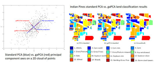
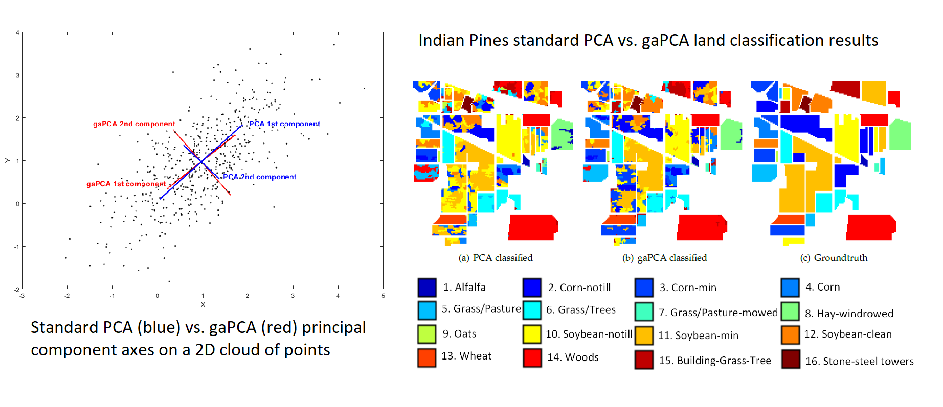
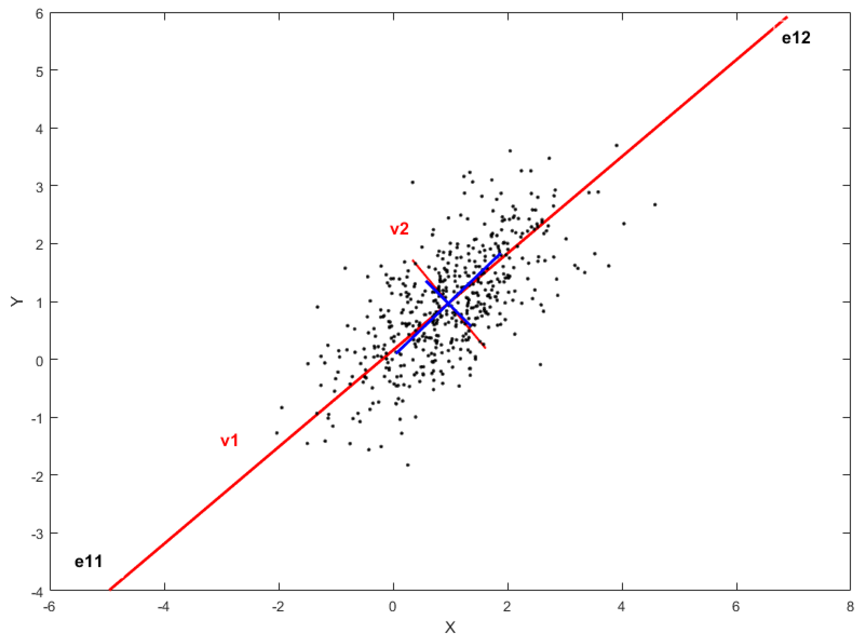
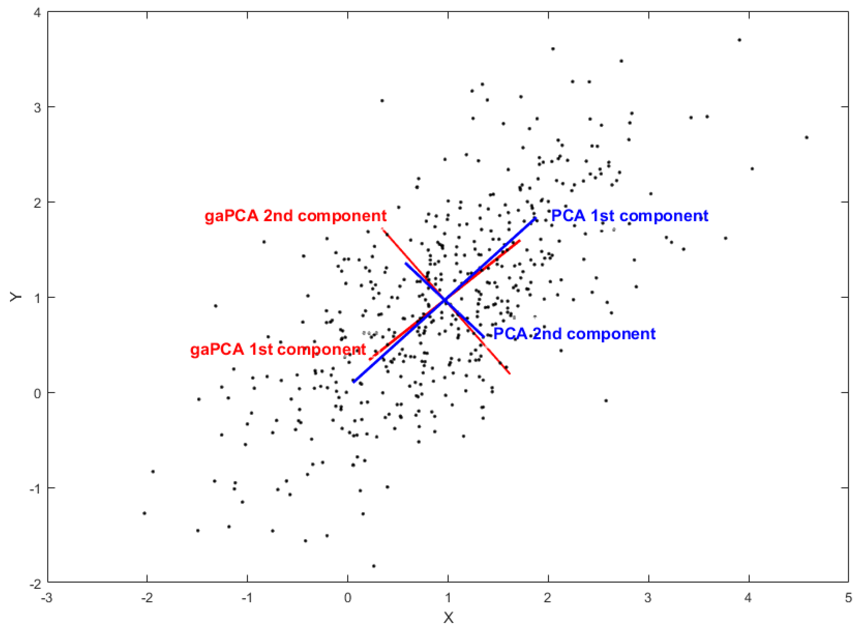
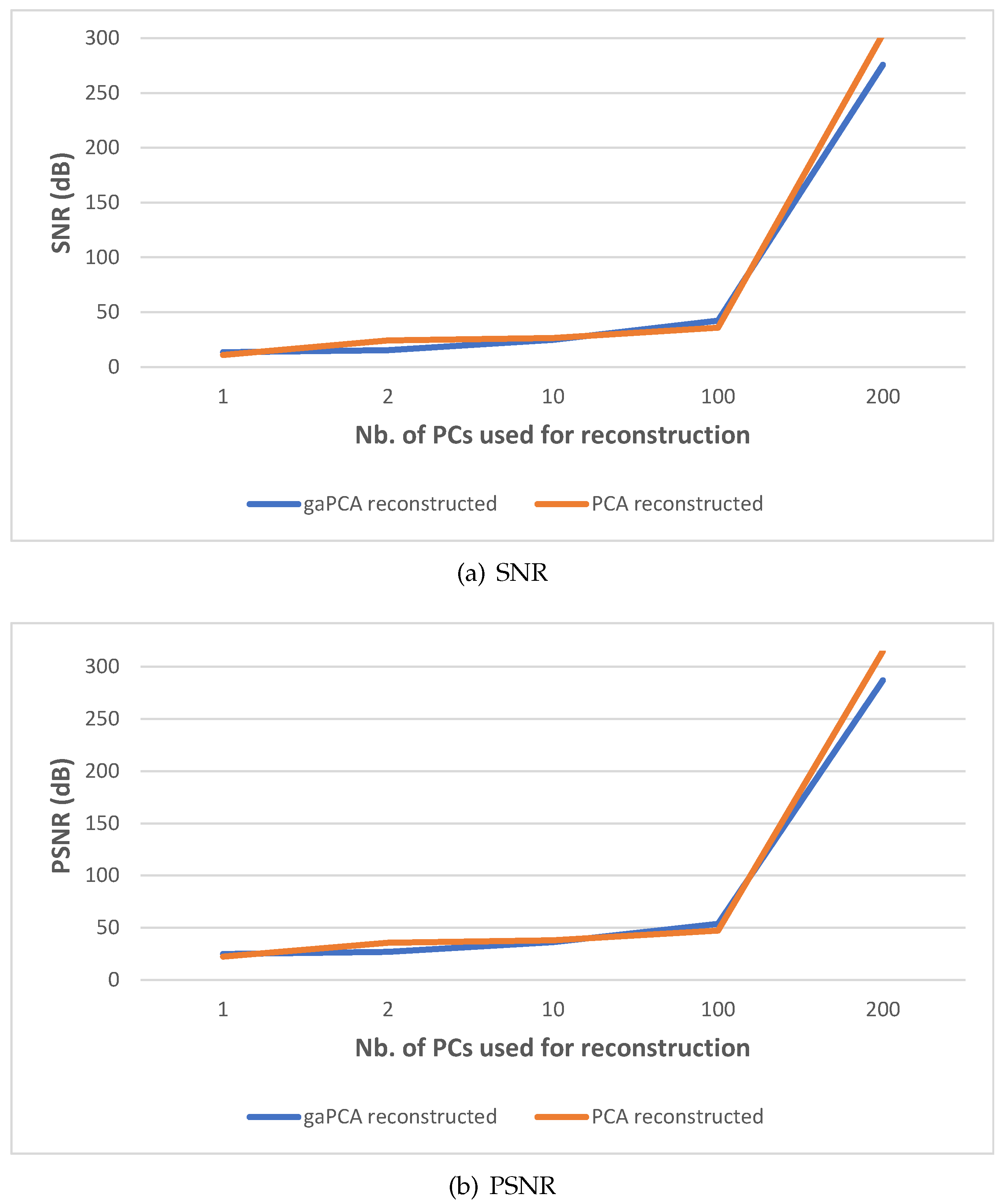
Figure 1 and Figure 2 illustrate the graphical comparison between gaPCA and standard PCA when computing the principal components on a set of randomly generated bidimensional points normally distributed. In both figures, the original points are depicted as black dots; the red lines represent the gaPCA principal components of the points, while the blue lines are the standard principal components. In Figure 1, the longer red line connects the two furthest points of the cloud of points ($e_{11}$ and $e_{12}$, separated by the maximum distance of all the distances computed between all the points) and represents the first gaPCA component ($v_1$). The shorter red line is orthogonal on the first red line and provides the second gaPCA component ($v_2$). Figure 2 depicts the normalized gaPCA vectors. One can notice the very high similarity of the red and blue lines, proving a close approximation of the standard PCA by the gaPCA method. The only visible difference is a small angle deviation.

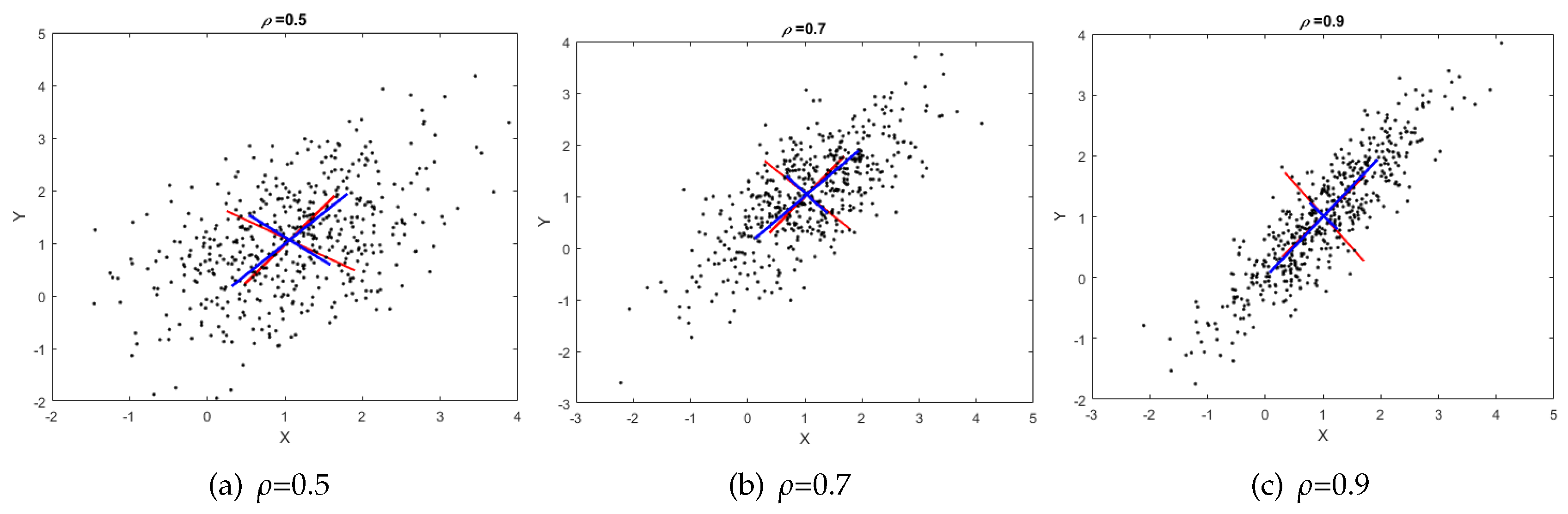
In Figure 3 three randomly-generated 2D points (in black), with the PCA represented with blue lines and gaPCA with red lines, for three values of the correlation coefficient: $\rho =$ 0.5, 0.7 and 0.9, respectively, are shown. One may notice that for higher values of the correlation parameter, angle deviation decreases to very small values. This shows that the stronger the correlation of the variables, the better the approximation provided by gaPCA. On the other hand, when the dataset is weakly correlated, PCA’s direction of the axes is purely arbitrary (since there is no significant maximum variance axis).

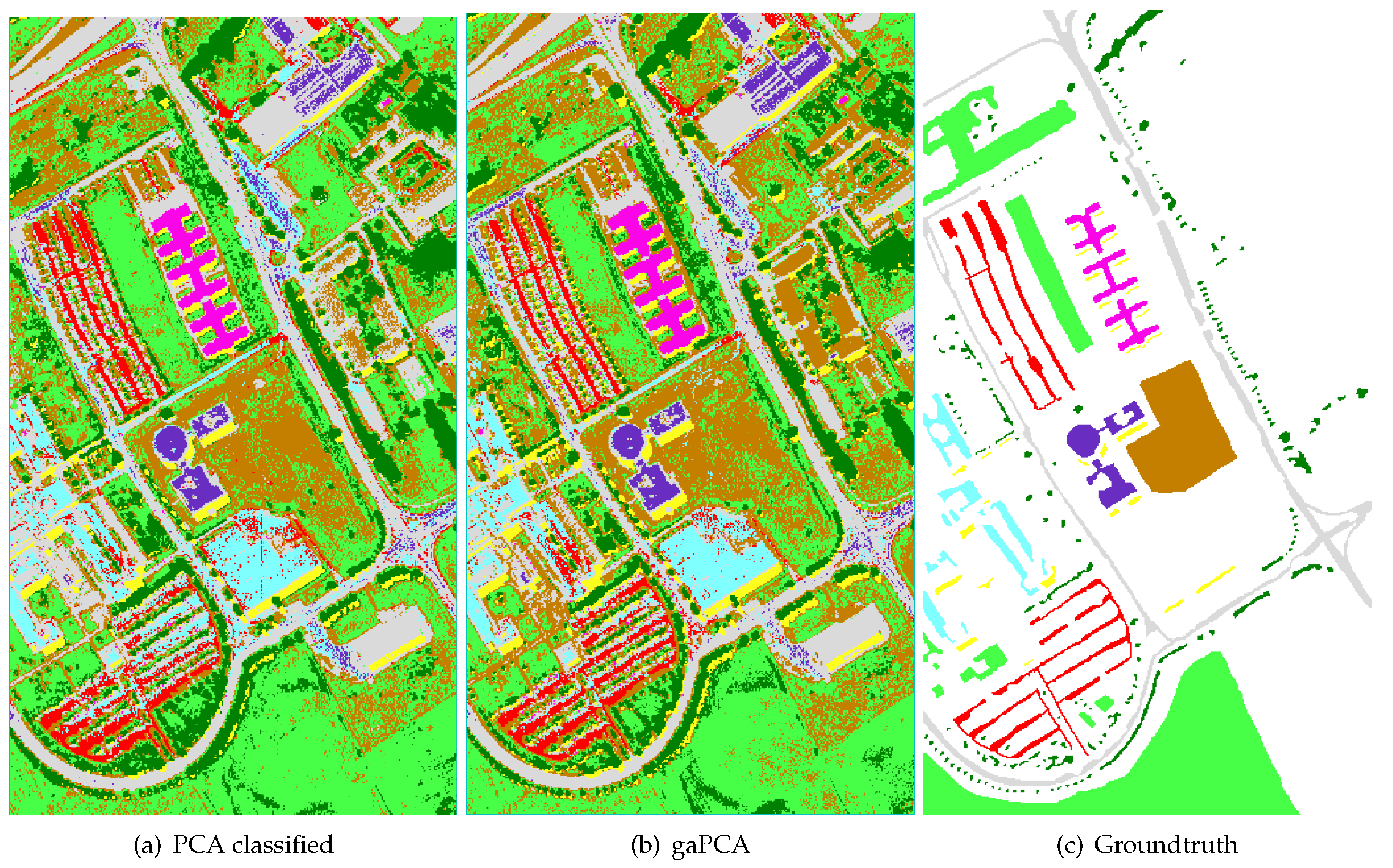
3.2. Datasets

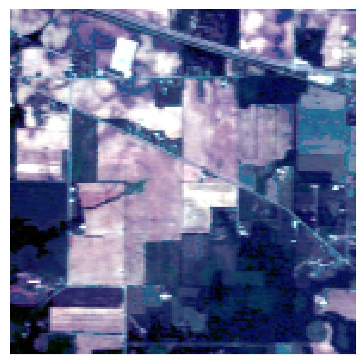
The first set of experimental data was gathered by AVIRIS sensor over the Indian Pines test site in the north-western Indiana and consists of 145 × 145 pixels and 224 (200 usable) spectral reflectance bands in the wavelength range 0.4–2.5 × 10^-6 m. The Indian Pines scene is a subset of a larger one and contains approximately 60 percent agriculture, and 30 percent forest or other natural perennial vegetation. There are two major dual-lane highways, a rail line, and some low density housing, other built structures, and smaller roads. The scene was taken in June and some of the crops present, corn, soybeans, are in early stages of growth with less than 5% coverage [30].

Figure 4 displays an RGB image of the Indian Pines dataset.

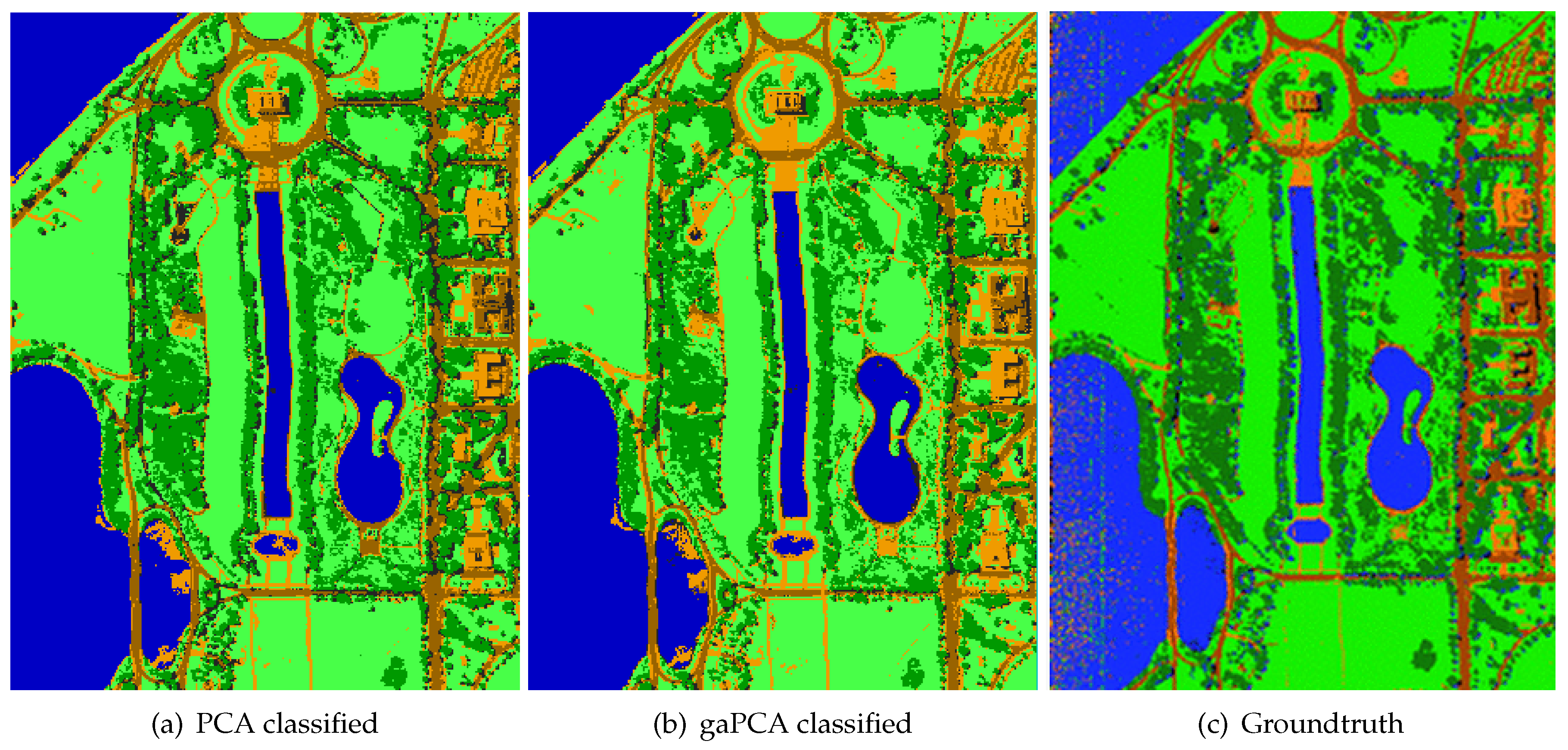
The second data set used for experimental validation was the Pavia University data set, acquired by the ROSIS sensor during a flight campaign over Pavia in northern Italy. The scene containing the Pavia University has a number of 103 spectral bands. Pavia University is a 610 × 340 pixels image with a geometric resolution of 1.3 m. The image ground-truth differentiates nine classes [31]. An RGB image of Pavia University is shown in Figure 5.

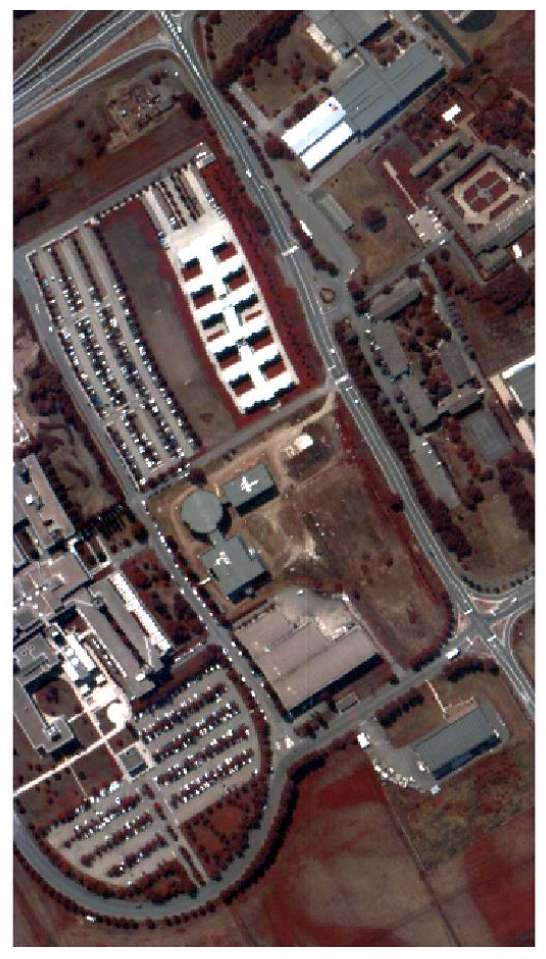
The third set of experimental data was collected by the HYDICE sensor over a mall in Washington DC. It has 1280 × 307 pixels with 210 (191 usable) spectral bands in the range of 0.4–2.4 $\mathsf{\mu }$m. The spatial resolution is 2 m/pixel. An RGB image of the DC Mall is shown in Figure 6.

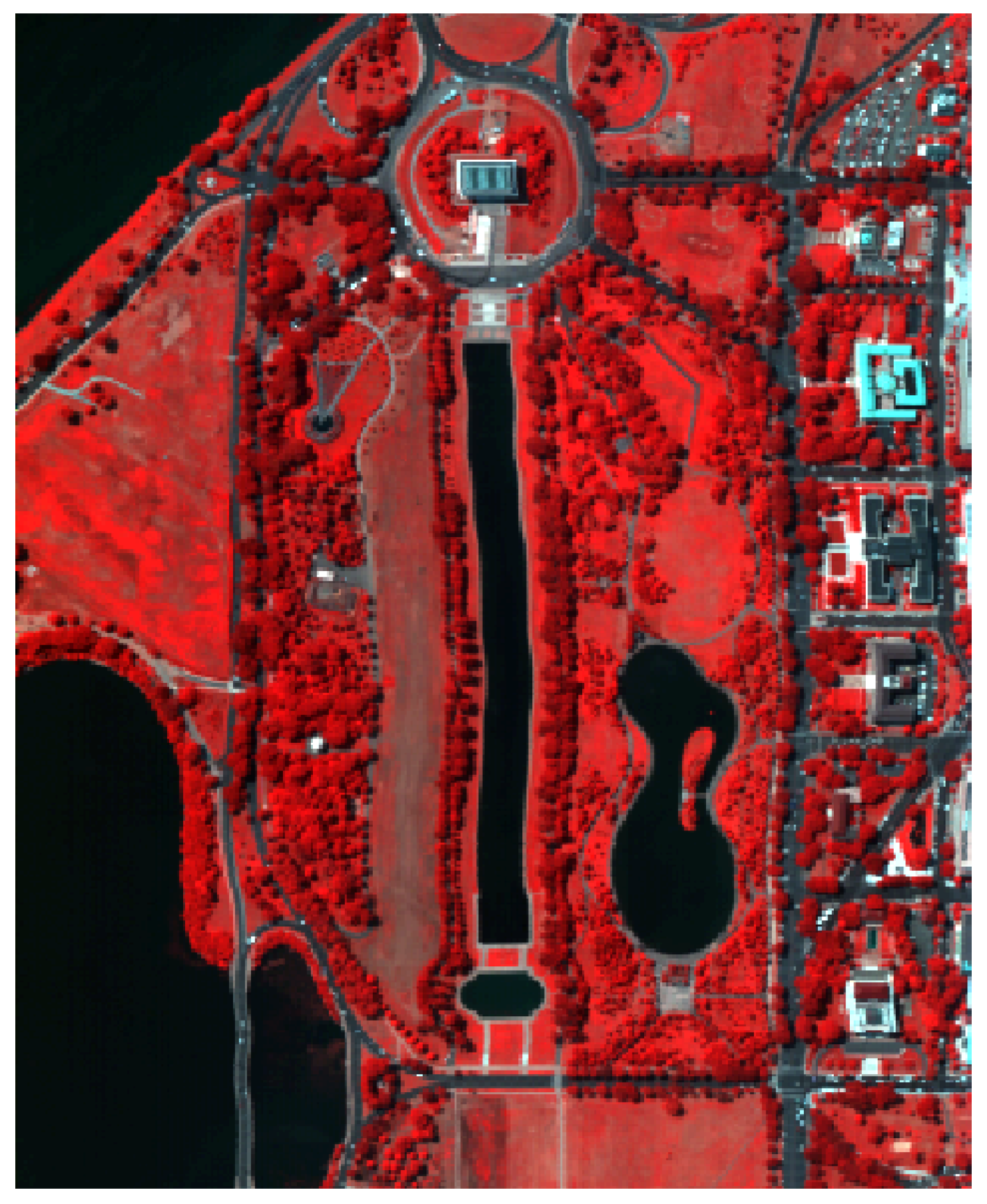
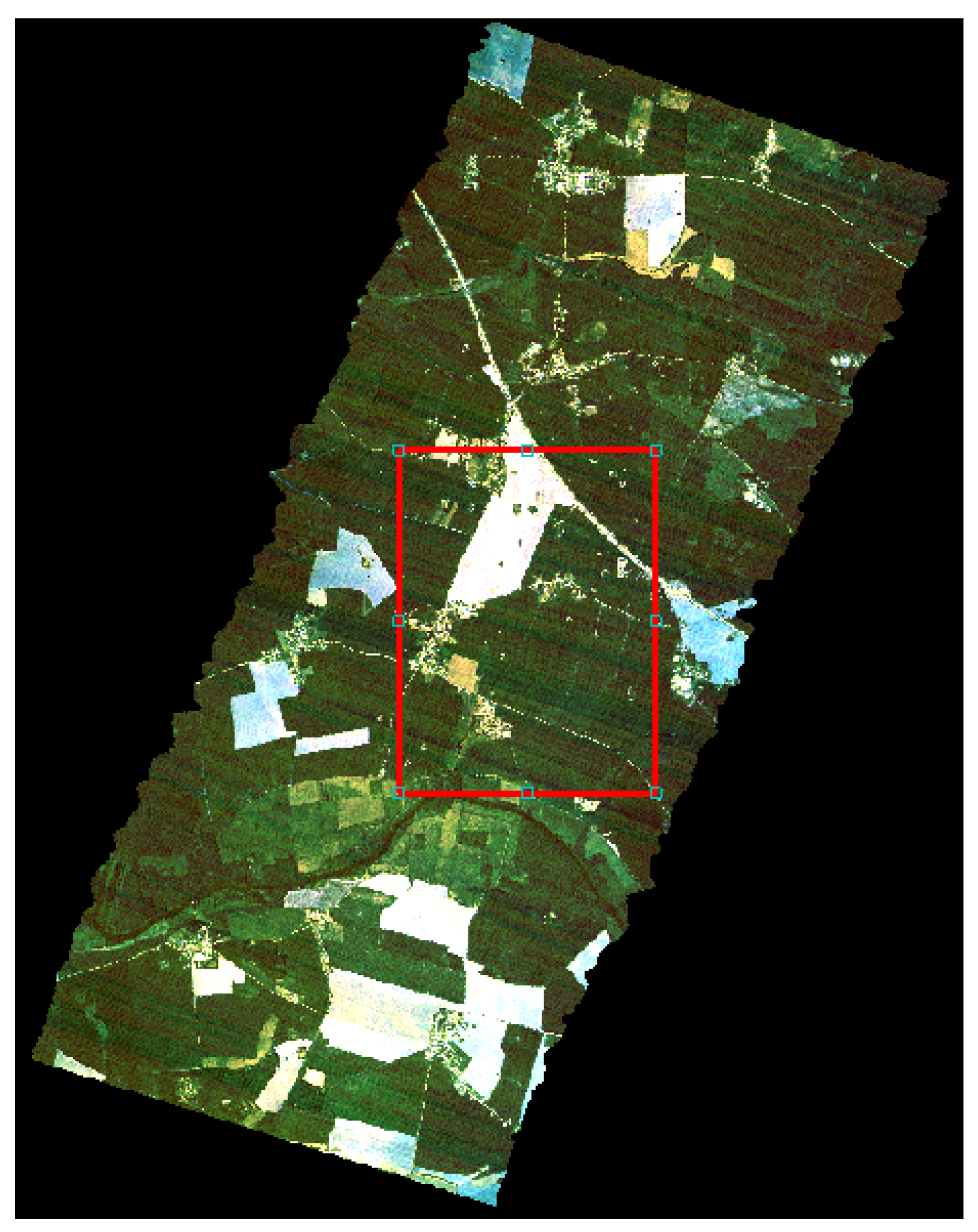
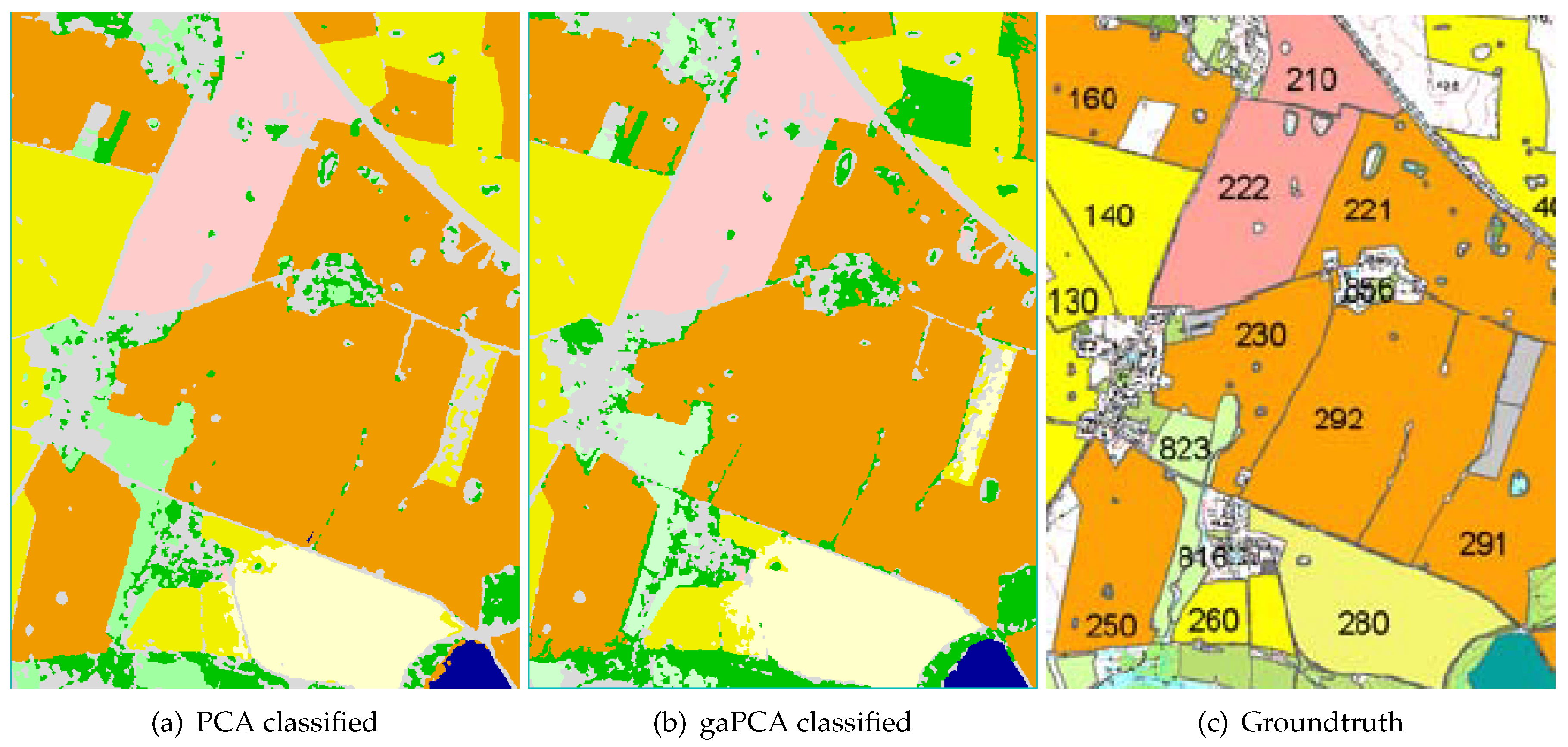
The fourth set of experimental data used in this research was acquired by the airborne INTA-AHS instrument in the framework of the European Space Agency (ESA) AGRISAR measurement campaign [32]. The test site is the area of Durable Environmental Multidisciplinary Monitoring Information Network (DEMMIN). This is a consolidated test site located in Mecklenburg–Western Pomerania, North-East Germany, which is based on a group of farms within a farming association, covering approximately 25,000 ha. The fields are very large in this area (in average, 200–250 ha). The main crops grown are wheat, barley, oilseed rape, maize, and sugar beet. The altitude range within the test site is around 50 m.

The AHS has 80 spectral channels available in the visible, shortwave infrared, and thermal infrared, with a pixel size of 5.2 m. For this research, the acquisition taken on the 6 June 2006, has been considered. At that time, five bands in the SWIR region became blind due to loose bonds in the detector array, so they were not used in this paper. An RGB image of the DEMMIN test site taken by the AHS instrument, also showing the image crop used in our experiments is illustrated in Figure 7.

3.3. Performance Evaluation

The gaPCA method’s results have been qualitatively and quantitatively evaluated, in terms of quality of the principal components images (Gray Level Co-Occurrence Matrix (GLCM) textural analysis metrics), quality of the reconstruction (Signal to Noise Ratio (SNR), Peak Signal to Noise Ratio (PSNR)), redundancy of the principal components (Mutual Information (MI)) and the land classification accuracy obtained on the gaPCA principal components.

3.3.1. Textural Analysis Metrics

Gray level co-occurrence matrix (GLCM) [33] texture is a powerful image feature for image analysis. For this analysis we use three GLCM parameters: energy, contrast and entropy. Energy (Equation (8)), also called angular second moment [34] and uniformity [35] measures textural uniformity (pixel pairs repetitions) [36]. Contrast, also known as spatial frequency, is the difference between the highest and the lowest values of a contiguous set of pixels (as expressed by Equation (7)). Entropy (Equation (9)) measures the complexity of an image [36].

These parameters are correlated with the image quality as follows: energy decreases whereas contrast and entropy increase with increasing image quality [36,37].

$$Contrast=\sum _{i=0}^{N_G-1}\sum _{j=0}^{N_G-1}{(i-j)}^2·G(i,j)$$

(7)

$$Energy=\sum _{i=0}^{N_G-1}\sum _{j=0}^{N_G-1}{G}^2(i,j)$$

(8)

$$Entropy=-\sum _{i=0}^{N_G-1}\sum _{j=0}^{N_G-1}G(i,j)·lo{g}_2\left(G(i,j)\right)$$

(9)

In the above equations (Equations (7)–(9)), G represents the gray level co-occurrence matrix, each entry of the matrix is denoted by $G(i,j)$ and represents the probability that the pixel with value i will be found adjacent to the pixel of value j [38]; $N_G$ is the number of distinct gray levels in the image.

3.3.2. Quality of the Reconstruction Metrics

In order to assess the quality of the reconstruction of the original image, we used the Signal to Noise Ratio (SNR) and Peak Signal to Noise Ratio (PSNR). This paper presents the SNR, PSNR, and MI results for the Indian Pines dataset, since the results for the other datasets are similar and support the same conclusion.

A widely used metric for assessing the quality of the reconstructed image is the Signal to Noise Ratio (SNR) computed as [39]:

$$SNR=10·lo{g}_{10}\frac{{\sum }_{i=1}^n{\sum }_{j=1}^{m}Y{(i,j)}^2}{{\sum }_{i=1}^n{\sum }_{j=1}^m{(Y(i,j)-X(i,j))}^2}$$

(10)

where {$X(i,j)$ is the spectral pixel vector of the original image and $Y(i,j)$ is the spectral pixel vector of the reconstructed image. The values of the SNR can be interpreted such as the higher the values, the closer the reconstructed image to the original one.

Another metric, related to SNR, is Peak Signal to Noise Ratio (PSNR) [39]:

$$PSNR=10·lo{g}_{10}\frac{peakva{l}^2}{{\sum }_{i=1}^n{\sum }_{j=1}^m{(Y(i,j)-X(i,j))}^2}$$

(11)

where $peakval$ is taken from the range of the image (e.g., $0\dots 255$ or $0\dots 1$) and $X(i,j)$ is the spectral pixel vector of the original image and $Y(i,j)$ is the spectral pixel vector of the reconstructed image; m and n are the total number of pixels in the horizontal and the vertical dimensions of the image.

3.3.3. Redundancy of the Principal Components Metric

Mutual Information is a statistical non-parametric complete dependency (both linear and nonlinear) measure, which mathematically evaluates the probabilistic dependence between two random variables using the concept of entropy. High and zero values of MI indicate that two random variables are dependent on each other and independent respectively [40]. It is widely used as a similarity measure for remote sensing images [41,42,43]. It is also used as an evaluation benchmark for dimensionality reduction techniques [44].

In our case the MI between each pair of principal components was computed for both methods in order to assess the amount of redundancy in the computed principal components of each method (the MI measures the information that the two variables share [44]). Differently from the PCA approach, in gaPCA the components are not ranked in terms of variance (or any other metric). A consequence of this is that the compressed information tends to be distributed among the components, and not concentrated in the first few like in the standard PCA.

The classical correlation coefficient was not used since the PCA is optimal for that criterion. For comparison, we used the normalized MI (NMI), defined as [45]:

$$NMI(X,Y)=\frac{MI(X,Y)}{\sqrt{H\left(X\right)}·\sqrt{H\left(Y\right)}}$$

(12)

where

$$MI(X,Y)=H\left(X\right)+H\left(Y\right)-H(X,Y)$$

(13)

In the above equations, $H\left(X\right)$ represents the entropy of a discrete random variable X:

$$H\left(X\right)=\sum _{x\in X}p\left(x\right) log p\left(x\right)$$

(14)

with $p\left(x\right)$ being the probability density function of x. $H(X,Y)$ is the joint entropy of X and Y (in our case, the principal components images), and is defined as:

$$H(X,Y)=-\sum _{x\in X y\in Y}p(x,y) log p(x,y)$$

(15)

with $p(x,y)$ being the joint probability density function of x and y.

The MI is usually used to assess the independence between two variables, and is a standard for the degree the information that the two variables share. Normalized Mutual Information (NMI) is a normalization score to scale the results between 0 (no mutual information) and 1 (100% similarity).

3.3.4. Classification Accuracy Assesment Metrics

On the grounds of PCA (among other methods) being successfully used in remote sensing for reducing the redundant data, for extracting specific land cover information or for performing feature extraction [46], we aimed at comparing the gaPCA approach in the field of classification with the standard PCA algorithm as the benchmark for the assessment of the gaPCA method.

For each data set, the number of principal components computed was selected in order to achieve the best amount of variance explained (98–99%) with a minimum number of components (10 for the Indian Pines data, 4 for Pavia University, 3 for DC Mall and 3 for AHS). The first principal components achieved after the implementation of each of the PCA methods represent the bands of the images on which the classification was performed (the input), using the ENVI [47] software application. For all of the data sets used, the Maximum Likelihood Algorithm (ML) and the Support Vector Machine Algorithm (SVM) were used for classifying both the standard PCA and the gaPCA image. The accuracy of each classification was assessed using the same randomly generated pixels and by visual comparison with the ground-truth image of the test site at the acquisition moment.

We assessed the classification accuracy of each method with two metrics: the overall accuracy (OA representing the number of correctly classified samples divided by the number of test samples) and the kappa coefficient of agreement (k, which is the percentage of agreement corrected by the amount of agreement that could be expected due to chance alone).

In order to assess the statistical significance of the classification results provided by the two methods, the McNemar’s test [48] was performed for each classifier (ML and SVM), based on the equation:

$$z=\frac{f_{12}-f_{21}}{\sqrt{f_{12}+f_{21}}}$$

(16)

where $f_{ij}$ represents the number of samples missclassified by method i, but not by method j. For $\left|z\right|>1.96$, the overall accuracy differences are said to be statistically significant.

4. Results and Discussion

4.1. GLCM Textural Analysis Metrics

After computing the principal components using standard PCA and gaPCA, we performed land classification on all four datasets (on the principal components images). In order to validate the hypothesis that gaPCA yields better classification results due to its enhanced ability to retain information in its principal components compared to the canonical PCA, we used a well-known image quality metric, namely the GLCM textural analysis to assess the amount of information in each method’s principal components.

The GLCM textural analysis metrics were used to assess the quality of the images represented by the principal components of each method. Since these images are the ones on which the actual land classification task is performed, we aimed to evaluate the quality of the images, and the amount of useful information contained by each of the images provided by the two methods, that could actually lead to better classification results. Each of the metric computed (contrast, energy, entropy), used the same number of components that were used in the experiments, (that is 10 for the Indian Pines, four for Pavia University, three for DC Mall and three for the AHS dataset, the same number for both methods).

The contrast computed for each of the retained principal components images and averaged for both methods for each dataset is provided in

Table 1. Gray Level Co-Occurrence Matrix (GLCM) contrast metric for both methods on all datasets.

	Indian Pines	Pavia University	DC Mall	AHS
PCA	0.96	0.14	0.25	0.17
gaPCA	0.34	0.12	0.32	0.18

. For two of the datasets (DC Mall and AHS) the gaPCA principal components held higher contrast values, on average, while for the other two datasets the results are reversed.

Table 2. GLCM energy metric for both methods on all datasets.

	Indian Pines	Pavia University	DC Mall	AHS
PCA	0.14	0.58	0.29	0.23
gaPCA	0.21	0.53	0.20	0.21

shows the energy-averaged values of the principal components images for both methods, for each dataset. The results show that in almost all cases (except for the Indian Pines dataset), the gaPCA principal components energy values are lower (thus better in terms of image quality) than those of the PCA.

Table 3. GLCM entropy metric for both methods on all datasets.

	Indian Pines	Pavia University	DC Mall	AHS
PCA	6.95	5.28	6.07	6.72
gaPCA	6.61	5.17	6.38	6.45

presents the entropy-averaged values of the principal components images for both methods, for each dataset. Like in the contrast case, gaPCA scored better (higher entropy values) for the DCMall and AHS datasets, while for the other two, PCA scored better.

Although from the contrast and entropy point of view, the two methods seem to produce similar results, the energy metric shows that gaPCA principal components have a better image spatial quality, which could actually lead to better classification results.

4.2. Quality of the Reconstruction Metrics

The SNR computed between the original image and the image reconstructed from the standard PCA or gaPCA principal components is provided in

Table 4. SNR for the Indian Pines dataset.

Method	1PC	2PC	10PC	100PC	200PC
gaPCA	13.47	15.39	24.84	42.19	275.66
PCA	10.97	24.33	26.46	35.86	303.67

and in figure Figure 8a. The number of principal components used for reconstruction varied from 1 to 200 for both methods.

The PSNR computed between the original image and the image reconstructed from the standard PCA or gaPCA principal components is provided in

Table 5. PSNR for the Indian Pines dataset.

Method	1PC	2PC	10PC	100PC	200PC
gaPCA	24.87	26.79	36.24	53.60	287.06
PCA	22.37	35.73	37.86	47.26	315.03

and in figure Figure 8b. Different numbers of principal components from 1 to 200 were used for both methods.

These results show that both methods scored similar results in terms of both SNR and PSNR of the reconstruction. Moreover, the shape of the slope is almost identical for the two methods. The values for both methods increase when increasing the number of components used for reconstruction. As the results show, the gaPCA performs better than PCA when only the first principal component is used for reconstruction, while PCA leads to better results when all the principal components are used.

To conclude, gaPCA scores similar results in terms of quality of the reconstruction, with slightly better results when using a certain number of principal components.

4.3. Redundancy of the Principal Components Metric

The MI computed for the PCA and gaPCA principal components are provided in Figure 9. The figure presents the MI matrices, which represents the MI for each pair of principal components with both methods (PCA and gaPCA), for the Indian Pines data set.

The figure shows greater values for the MI between the PCA components (yellow and orange patches) than for those of the gaPCA algorithm. This shows that a higher degree of information is shared by principal components and consequently less new information is provided. Because the gaPCA principal components are not sorted by any criteria, there tends to be an amount of redundancy between the first components, still, the figure shows that more non-redundant information can be provided by the gaPCA components than by those of the PCA. Moreover, in the next sections we will show that the information provided by the gaPCA can be very useful for the purpose of classification.

4.4. Land Classification Accuracy

4.4.1. Indian Pines Dataset

The classification task of the Indian Pines dataset is a challenging one due to the large number of classes on the scene and the moderate spatial resolution of 20 m and also due to the high spectral similarity between the classes, the main crops of the region (soybeans and corn) being in an early stage of their growth cycle. The classification results of the Standard PCA and the gaPCA methods are shown in Figure 10a,b along with the ground-truth of the scene at the time of the acquisition of the image (c). From this figure, it can be seen that although both classified images look noisy (because of the abundance of mixed pixels ), the classification map obtained by the gaPCA is slightly better.

In

Table 6. Classification results for the Indian Pines dataset.

Class	Training Pixels	PCA ML	gaPCA ML	PCA SVM	gaPCA SVM
Alfalfa	32	98.7	80.5	18.2	18.2
Corn notill	1145	30.6	47.6	65.2	69.3
Corn mintill	595	51.6	69.2	34.9	46.1
Corn	167	84.9	100	31.4	37.7
Grass pasture	328	55.7	80.5	64.6	71.9
Grass trees	463	96.1	90.6	91.2	92.5
Grass pasture mowed	19	68.3	71.7	60	60
Hay windrowed	528	88.5	96.7	99.5	99.6
Oats	20	100	96.9	15.6	6.3
Soybean notill	681	83.7	77.1	40.9	56.1
Soybean mintill	1831	46.6	47.7	79.4	78.3
Soybean clean	457	36.9	77.7	11.8	36.1
Wheat	150	97.2	97	91.1	93.1
Woods	884	98.7	96.9	97.3	97.3
Buildings Drives	263	33.7	61.4	45.5	52.1
Stone Steel Towers	103	100	100	95.5	97.2
zML = 25.1 (signif = yes)	OA(%)	62.1	70.2	67.2	72.1
zSVM = 24.8 (signif = yes)	Kappa	0.57	0.67	0.62	0.68

we summarized the classification accuracy of the two methods for each of the classes on the scene along with the overall accuracy of both methods with the Maximum Likelihood (ML) and Support Vector Machine (SVM) algorithms. We used 20,000 randomly generated pixels, uniformly distributed in the entire image for testing. The gaPCA overall accuracy was superior to the one scored by the standard PCA and the classification accuracy results for most classes was better. This may be explained by the fact that PCA makes the assumption that the features that present high variance are more likely to provide good discrimination between classes, while those with low variance are redundant. This can sometimes be erroneous, like in the case of spectral similar classes. There is a substantial difference in the case of sets of similar class labels. gaPCA scored higher accuracy results for the similar sets of corn, corn notill, corn mintill, and also for grass-pasture and Grass-pasture mowed than those achieved by the Standard PCA, due to the ability of the method to better discriminate between similar spectral signatures.

4.4.2. Pavia University Dataset

Figure 11 shows the images achieved with the Standard PCA method (a) and the gaPCA method (b) classified with the Maximum Likelihood Algorithm of Envi software and the ground-truth of the scene (c).

The classification results (for 1000 test pixels) using either ML or SVM are displayed in

Table 7. Classification results for the Pavia University dataset.

Class	Training Pixels	PCA ML	gaPCA ML	PCA SVM	gaPCA SVM
Asphalt (grey)	1766	60.5	61.5	67.2	78.3
Meadows (light green)	2535	68.3	80	65	86.9
Gravel (cyan)	923	100	100	33.3	40
Trees (dark green)	599	88.2	89.7	100	67.7
Metal sheets (magenta)	872	100	100	100	100
Bare soil (brown)	1579	77.8	79.4	53.2	68.3
Bitumen (purple)	565	89.7	89.7	89.7	55.2
Bricks (red)	1474	68.3	72	81.7	86.6
Shadows (yellow)	876	100	100	100	100
zML = 4.87 (signif = yes)	OA(%)	72.2	78	69	78
zSVM = 5.97 (signif = yes)	Kappa	0.65	0.72	0.61	0.72

, showing the classification accuracy for each class and the overall accuracy. One can easily notice that the gaPCA scored the best overall accuracy and classification accuracy for most classes.

The classification accuracies report better performances for gaPCA in interpreting classes with small structures and complex shapes (e.g., asphalt, bricks). This may be explained by the interest accorded by the gaPCA to smaller object and spectral classes leading to less false predictions compared to the standard PCA for these classes. This is more prominent for classes such as bricks where confusion matrix shows a misinterpretation with gravel and for asphalt confused with bitumen.

This confusion can be attributed to the spectral similarity between the two classes and not to the spatial proximity (

Table 8. Excerpt from the confusion matrix for the Pavia University dataset.

Class	True	False
Asphalt (PCA)	60.5 Asphalt	29.5 Bitumen
Asphalt (gaPCA)	61.5 Asphalt	21.8 Bitumen
Meadows (PCA)	68.3 Meadows	25.8 Bare soil
Meadows (gaPCA)	80 Meadows	17.6 Bare soil
Bricks (PCA)	68.3 Bricks	25.6 Gravel
Bricks (gaPCA)	72 Bricks	24.3 Gravel

), proving that gaPCA does a better job in discriminating between similar spectral classes because unlike PCA it is not focused on classes that dominate the signal variance.

In light of these results, gaPCA is shown to have a consistent ability when classifying smaller objects or spectral classes, confirming the hypothesis that it has superior ability to retain information associated with smaller signals’ variance.

4.4.3. DC Mall Dataset

Figure 12 displays the images, obtained with the Standard PCA (a) and the gaPCA (b) method, classified with the Maximum Likelihood Algorithm of Envi software and the ground-truth of the DC Mall scene (c).

The classification accuracies (achieved both with ML and SVM) over different classes along with the overall accuracy (for 140 test pixels) of both methods for the DC Mall dataset are displayed in

Table 9. Classification results for the DC Mall dataset.

Class	Training Pixels	PCA ML	gaPCA ML	PCA SVM	gaPCA SVM
Road (dark brown)	862	90	100	100	100
Trees (dark green)	413	75.9	82.7	75.9	75.9
Water (blue)	466	86.7	83.3	86.7	86.7
Grass (light green)	992	86.9	91.3	67.4	71.7
Shadows (black)	121	87.5	75	37.5	50
Roofs and paths(brown)	358	64.7	94.1	52.9	52.9
zML = 2 (signif = yes)	OA(%)	82	88	72	74
zSVM = 1.13 (signif = no)	Kappa	0.77	0.85	0.65	0.67

. These results show that gaPCA outperforms the standard PCA algorithm in terms of overall accuracy and kappa. As for the Pavia University, gaPCA scores better in the case of small structures with complex shapes, such as roofs and paths, for which it exceeds the standard PCA with more than 30 percents. Trees are another preponderantly spectral class in the case of which the standard PCA’s accuracy is surpassed by the gaPCA’ due to its superior ability in preserving information related to this particular class. The overall accuracy is also higher in the case of the gaPCA approach by more than 5 percents.

4.4.4. AHS Dataset

For this particular dataset, the classification maps obtained after the computation of the standard PCA method and the gaPCA approach reveal relatively homogeneous regions as shown in Figure 13.

The corresponding classification class accuracy and overall accuracy of each PCA method for both ML and SVM, reported in

Table 10. Classification results for the AHS dataset.

Class	Training Pixels	PCA ML	gaPCA ML	PCA SVM	gaPCA SVM
Oilseed rape (dark yellow)	2786	93.3	93.3	93.2	97.7
Oilseed rape (light yellow)	1013	80	80	90	95
Maize (pink)	969	100	100	100	100
Winter wheat (orange)	4429	100	98.1	97.3	97.3
Pasture (light green)	1788	66.7	66.7	84.6	92.3
Grassland (dark green)	1242	60	80	52.4	95.2
Urban (grey)	1079	60	90	64	92
zML = 1.97 (signif = yes)	OA(%)	90.6	93.8	90	96.6
zSVM = 3.92 (signif = yes)	Kappa	0.86	0.91	0.86	0.95

and computed on the base of the ground-truth for 100 test pixels, shows a higher percentage of pixels correctly classified for the most classes for the gaPCA algorithm.

The results also report the differences in classification accuracies for both methods. It can easily be seen the high similarities between the standard PCA and gaPCA for the most extensive represented classes of the scene (oilseed rape, maize, set aside:oilseed rape). Low differences arise in the classes winter wheat, while the grassland and cutting pasture classes, which are known as preponderantly spectral classes, scored the lowest values. The urban class seems to be the most confusing and difficult to classify due to the specifics of these classes comprising a mix of buildings, country roads and vegetation in a rural area. Once again, the results show the gaPCA’s superior ability in classifying smaller spectral classes (e.g., Grassland) or similar and mixed pixels.

The McNemar’s test (z score) confirms for all datasets (with one isolated exception) the consistency of the gaPCA accuracy improvement over the standard PCA.

For obtaining the results shown above, all computations were executed in Matlab R2018b and ENVI 5.5, running on an AMD Ryzen 5 3600 and NVIDIA GeForce GTX 1650 system with 16 GB installed memory. As for the computational times, for the Indian Pines dataset, the total runtime of the gaPCA for computing one principal component was approximately 5 seconds, and under 1 minute for the first 10 principal components.

5. Conclusions

In this paper, a novel PCA approximation method based on a geometric construction approach (gaPCA) was introduced, with applications in hyperspectral remote sensing data analysis—more specific in land classification. The gaPCA method was validated on four experimental datasets consisting of remote sensing data, and the results yielded by the gaPCA method were qualitatively and quantitatively evaluated, in terms of image quality of the principal components provided and in terms of the land classification accuracy obtained on the gaPCA principal components.

As references for benchmarking, the standard PCA algorithm was used. The comparative evaluation with standard PCA was performed first by using several metrics: contrast, energy and entropy of the principal components images, SNR and PSNR between the original and reconstructed images and MI between the principal components.

Furthermore, the validation aimed to assess the performance of the proposed method from the point of view of its efficiency in the field of land classification of the remote sensing images. We performed a classification in order to evaluate the performances of the gaPCA method with those achieved by the standard PCA algorithm. In terms of classification accuracy, gaPCA scored on average higher than the standard method. The most remarkable results were recorded in the cases of preponderantly spectral classes, small objects or classes, where the standard PCA’s performances are lower due to its loss of information considered “unimportant" or redundant due to its small contribution to the overall signal variance, that restrain its ability to discriminate small objects or classes with fine similarities.

Consequently, gaPCA was shown to be more suitable for hyperspectral images with small structures or objects that need to be detected or where preponderantly spectral classes or spectrally similar classes are present.