Fast Split Bregman Based Deconvolution Algorithm for Airborne Radar Imaging

Abstract

Deconvolution methods can be used to improve the azimuth resolution in airborne radar imaging. Due to the sparsity of targets in airborne radar imaging, an $L_1$ regularization problem usually needs to be solved. Recently, the Split Bregman algorithm (SBA) has been widely used to solve $L_1$ regularization problems. However, due to the high computational complexity of matrix inversion, the efficiency of the traditional SBA is low, which seriously restricts its real-time performance in airborne radar imaging. To overcome this disadvantage, a fast split Bregman algorithm (FSBA) is proposed in this paper to achieve real-time imaging with an airborne radar. Firstly, under the regularization framework, the problem of azimuth resolution improvement can be converted into an $L_1$ regularization problem. Then, the $L_1$ regularization problem can be solved with the proposed FSBA. By utilizing the low displacement rank features of Toeplitz matrix, the proposed FSBA is able to realize fast matrix inversion by using a Gohberg–Semencul (GS) representation. Through simulated and real data processing experiments, we prove that the proposed FSBA significantly improves the resolution, compared with the Wiener filtering (WF), truncated singular value decomposition (TSVD), Tikhonov regularization (REGU), Richardson–Lucy (RL), iterative adaptive approach (IAA) algorithms. The computational advantage of FSBA increases with the increase of echo dimension. Its computational efficiency is 51 times and 77 times of the traditional SBA, respectively, for echoes with dimensions of $218\times 400$ and $400\times 400$, optimizing both the image quality and computing time. In addition, for a specific hardware platform, the proposed FSBA can process echo of greater dimensions than traditional SBA. Furthermore, the proposed FSBA causes little performance degradation, when compared with the traditional SBA.

1. Introduction

High-resolution airborne radar imagery are beneficial for obtaining accurate target information of imaging regions in many applications in the military and civilian fields, such as precise guidance of weapons, autonomous landing of aircraft, topographic mapping, and so on. In these applications, the radar usually works in scanning mode. The radar antenna actively transmits a large bandwidth signal, such as a linear frequency modulated (LFM) signal, to scan the imaging area along with the movement of the platform, obtaining surface information of the imaging area through signal reflection. Range resolution can be easily improved by pulse compression and range walk correction. However, its azimuth resolution is limited by the antenna size [1,2,3], which greatly restricts radar imaging performance.

According to the radar imaging theory, high azimuth resolution requires a large antenna aperture, which is usually unrealistic in practice due to the limitations of the platform. As a result, many researchers have devoted effort to improving the azimuth resolution by signal processing methods. It has been verified that the azimuth signal in airborne radar imaging can be modeled as a convolution of a target distribution and an antenna pattern [4,5,6], such that the azimuth resolution can be improved by deconvolution methods. However, as attributable to the ill-posedness of deconvolution, its inverse is highly sensitive to noise. Although many methods have been presented to relax the ill-posedness of deconvolution, such as Wiener filtering (WF) [7], truncated singular value decomposition (TSVD) [8], Tikhonov regularization (REGU) [9], Richardson–Lucy (RL) [10], iterative adaptive approach (IAA) [11], and so on, they have only achieved limited resolution improvement in airborne radar imaging.

Recently, sparse regularization has been proposed as another effective method to overcome the ill-posedness of decovolution and improve the azimuth resolution in airborne radar imaging [12,13,14]. In this method, the problem of azimuth resolution improvement is transformed into an optimization problem by introducing the sparse constraint of the target distribution in the regularization framework, where the distribution of the target is obtained by solving the optimization problem. In airborne radar imaging, the target of interest is usually sparse, compared with whole imaging region; therefore, the sparse regularization method is suitable for improving the azimuth resolution. In the regularization framework, the introduction of the $L_0$ norm of a target can lead to strong sparsity; however, solving this problem is $NP$-hard. A reasonable substitution is the $L_1$ norm of the target [15,16], which leads an $L_1$ regularization problem. The solution of the $L_1$ regularization problem is the estimated target distribution we need.

In reality, solving an $L_1$ regularization problem is a challenging task, as the $L_1$ norm is not differentiable. In recent studies, the split Bregman algorithm (SBA) has been widely utilized to solve the non-differentiable $L_1$ regularization problem, obtaining good effect in many fields such as optical imaging [17,18], radar imaging [19,20], compressed sensing [21,22], computed tomography (CT) [23,24], magnetic resonance imaging (MRI) [21,25], and so on. However, in this process, it is necessary to invert a coefficient matrix, resulting in high computational costs due to the computational complexity of matrix inversion, which is $O\left(N^3\right)$. The acceleration methods need to be researched.

To accelerate an algorithm, some strategies have been studied [26,27,28]. These strategies are designed to reduce iterations. However, due to the high computational costs of SBA is not caused by too many iterations, these strategies can not effectively increase the efficiency of SBA. In order to solve the problem of high computation cost caused by matrix inversion, researchers typically wish to realize fast inversion by utilizing special structures of coefficient matrix to avoid the inversion operation, such as Toeplitz structure, Hankel structure, and so on [29,30,31]. In previous research, we found that the coefficient matrix has a Toeplitz structure when using SBA to solve the $L_1$ regularization problem.

In Reference [32], T. Kailath proposed the concepts of displacement structure and displacement rank, as well as revealing that the operation can be compressed by using a Toeplitz matrix. It has been proven that the displacement rank of a Toeplitz matrix is very small and, so, its inverse matrix also has a displacement structure, which laid the theoretical foundation for the fast solution of Toeplitz equations [33]. Recently, utilizing the low displacement rank features of Toeplitz matrices, along with the Gohberg–Semencul (GS) representation, the fast inversion of Toeplitz matrices has been studied [30,34,35].

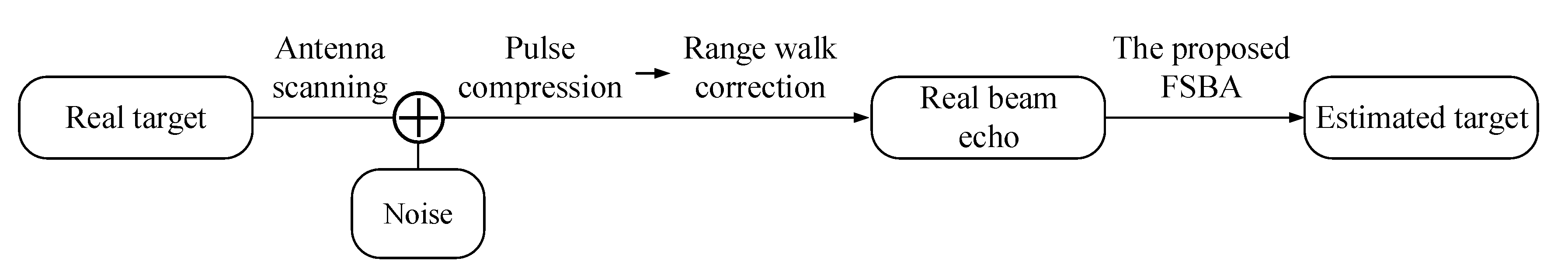
Focusing on the improvement of azimuth resolution and real-time imaging ability for airborne radar, a fast split Bregman algorithm (FSBA) is proposed in this paper. The signal processing scheme of this paper is shown in Figure 1, where the rounded rectangle represents the signal data. We first analyze the imaging process in airborne radar imaging. After antenna scanning, pulse compression, and range walk correction, the real beam echo can be expressed as a convolution between a target distribution and an antenna pattern. Secondly, the problem of azimuth resolution improvement is converted into an $L_1$ regularization problem by introducing the $L_1$ norm as a penalty in the regularization framework. Thirdly, based on the low displacement rank features of Toeplitz matrices, along with the GS representation, the traditional SBA is accelerated to solve the $L_1$ regularization problem, where its solution is the estimated target. After acceleration, the computation complexity is greatly reduced. Finally, the simulation and real data are used to verify the performance of the proposed algorithm.

The remainder of this paper is structured as follows. In Section 2, we analyze the signal model in airborne radar imaging and deduce the $L_1$ regularization problem. In Section 3, the proposed FSBA is derived, in detail, to solve the $L_1$ regularization problem. In Section 4, simulated and real data are exploited to demonstrate the performance of the proposed method. Finally, the conclusion is discussed in Section 5.

2. Problem Formulation

In this section, we deduce the signal model of airborne radar imaging and present the $L_1$ regularization problem.

2.1. Signal Model

In airborne radar imaging, the radar antenna actively transmits an electromagnetic wave to scan the imaging area along the direction of movement of the platform. In range dimension, the resolution depends on the bandwidth of the transmitted signal; that is, ${\rho }_r=c/\left(2B\right)$, where ${\rho }_r$ denotes the range resolution, c is the speed of light, and B is the bandwidth of the transmitted signal. It can be seen that a higher range resolution needs a larger bandwidth. Furthermore, in radar imaging, the working distance is typically large and requires a large time width of the transmitting signal. Therefore, in order to take into account both range resolution and working distance, the LFM signal is usually exploited as a transmitting signal in airborne radar imaging, due to its large time-bandwidth product. After pulse compression, the resolution in range dimension is much higher than that in azimuth dimension. In addition, in moving platform imaging, the targets of the same range bin are dispersed into different range bins, such that range walk correction is required after pulse compression.

In azimuth dimension, the echo is related to antenna scanning. For a radar system, the sampling point (in azimuth) can be expressed as

$$N={\displaystyle \frac{\mathsf{\Phi }}{\omega }}PRF,$$

(1)

where N is the sampling points in azimuth, $\mathsf{\Phi }$ is the scanning region, and $\omega$ is the scanning speed.

After pulse compression and range walk correction, the azimuth echo can be modeled as a convolution between a target distribution and an antenna pattern.

In practice, the noise cannot be avoided. Considering additive white Gaussian noise, the convolution model of the azimuth echo is

$$\mathit{y}=\mathit{h}\otimes \mathit{f}+\mathit{n},$$

(2)

where $\mathit{y}={\left[\begin{array}{cccc}{y}_1& y_2& \cdots & y_N\end{array}\right]}^T$ and $\mathit{f}={\left[\begin{array}{cccc}{f}_1& f_2& \cdots & f_N\end{array}\right]}^T$ are the azimuth echo and target distribution for one range bin, respectively; $\mathit{h}={\left[\begin{array}{cccc}{h}_1& h_2& \cdots & h_L\end{array}\right]}^T$ is the antenna pattern; $\mathit{n}$ is the noise; and ⊗ is the convolution operator.

The convolution of Equation (2) can be written as matrix vector multiplication:

$$\mathit{y}=\mathit{H}\mathit{f}+\mathit{n},$$

(3)

where $\mathit{H}$ is a circular matrix which is structured by an antenna pattern,

$$\mathit{H}=\left[\begin{array}{cccc}{h}_1& 0& \cdots & 0\\ h_2& h_1& \ddots & ⋮\\ ⋮& h_2& \ddots & 0\\ h_L& ⋮& \ddots & h_1\\ 0& h_L& ⋮& h_2\\ ⋮& \ddots & \ddots & ⋮\\ 0& \cdots & 0& h_L\end{array}\right].$$

(4)

From model (3), the target distribution $\mathit{f}$ can be obtained, typically by least squares (LS) estimation; that is,

$$\widehat{\mathit{f}}={\left({\mathit{H}}^T\mathit{H}\right)}^{-1}{\mathit{H}}^T\mathit{y},$$

(5)

where $\widehat{\mathit{f}}$ is the estimation of $\mathit{f}$. However, the problem of recovery by Equation (5) is typically ill-posed. Therefore, the perturbation caused by the noise may cause the estimated $\widehat{\mathit{f}}$ to be far from the true values.

2.2. Regularization Problem

Regularization is a method that effectively relaxes the ill-posedness. The optimization model can be expressed as

$$\widehat{\mathit{f}}=\underset{\mathit{f}}{min}\left[\frac{\mu }{2}{∥\mathit{H}\mathit{f}-\mathit{y}∥}_2^2+R\left(\mathit{f}\right)\right],$$

(6)

where ${∥\mathit{H}\mathit{f}-\mathit{y}∥}_2^2$ is the LS term used to measure the fitting degree between estimated value $\widehat{\mathit{f}}$ and real target $\mathit{f}$, and $R\left(\mathit{f}\right)$ is the regularization term. In particular, the regularization model degenerates to LS estimation if $R\left(\mathit{f}\right)=0$, and can be solved by Equation (5); however, this method is susceptible to noise interference due to the ill-posedness. Furthermore, $\mu$ is a regularization parameter, which is used to balance between LS and regularization terms.

In general, the selection of the regularization term relies on prior information. Based on different imaging scenes, the resolution can be improved by introducing a reasonable regularization term. Recently, many regularization technologies have been proposed, based on different regularization terms $R\left(\mathit{f}\right)$. For example, the REGU [9], total variation (TV) [36], and low rank (LR) [37] methods, among others.

In airborne radar imaging, we typically are only concerned with some strong targets. These strong targets occupy only a small part of the entire imaging scene and are usually sparse. Under the sparsity assumption, the recovery of a target $\mathit{f}$ requires solving the following optimization problem:

$$\widehat{\mathit{f}}=\underset{\mathit{f}}{min}{\displaystyle \frac{\mu }{2}}{∥\mathit{H}\mathit{f}-\mathit{y}∥}_2^2+{∥\mathit{f}∥}_0,$$

(7)

where ${∥\mathit{f}∥}_0$ represents the number of non-zero elements in $\mathit{f}$. However, the optimization problem (7) is $NP$-hard and is generally impossible to solve, as its solution usually requires an intractable combinatorial search.

As an alternative, a common $L_1$ regularization problem has been proposed:

$$\widehat{\mathit{f}}=\underset{\mathit{f}}{min}{\displaystyle \frac{\mu }{2}}{∥\mathit{H}\mathit{f}-\mathit{y}∥}_2^2+{∥\mathit{f}∥}_1,$$

(8)

where ${∥\mathit{f}∥}_1=\sum \left|f_i\right|$.

Unlike (7), the problem (8) is convex, such that it can be effectively solved by convex optimization methods. However, as the $L_1$ norm is not differentiable, finding its solution is challenging.

3. Solution of the Optimization Problem

In this section, we utilize the traditional SBA to obtain the solution of the $L_1$ regularization problem (8). The proposed FSBA will be derived in detail.

3.1. Solution with SBA

The SBA has been introduced in previous research. To solve problem (8), first, a variable $\mathit{d}$ was used to replace $\mathit{f}$:

$$\begin{array}{c}\widehat{\mathit{f}}=\underset{\mathit{f}}{min}{\displaystyle \frac{\mu }{2}}{∥\mathit{H}\mathit{f}-\mathit{y}∥}_2^2+{∥\mathit{d}∥}_1\hfill \\ s.t\mathit{d}=\mathit{f}.\hfill \end{array}$$

(9)

As (9) is a constrained problem, it is not easy to obtain its optimal solution. Therefore, we relax the constraints by using a penalty function continuation method:

$$\widehat{\mathit{f}}=\underset{\mathit{f}}{min}{\displaystyle \frac{\mu }{2}}{∥\mathit{H}\mathit{f}-\mathit{y}∥}_2^2+{\displaystyle \frac{\lambda }{2}}{∥\mathit{d}-\mathit{f}∥}_2^2+{∥\mathit{d}∥}_1,$$

(10)

where $\lambda$ is a positive parameter of penalty function weights. It seems that (9) and (10) are redundant on the surface; however, they can reduce the computational complexity extremely and lead to more efficient iterative strategies.

Another important notion is the Bregman distance for the SBA. For a convex functional defined on a Hilbert space J, its Bregman distance between points $\mathit{u}$ and $\mathit{v}$ is defined as

$$D_J^{\mathit{p}}\left(\mathit{u},\mathit{v}\right)=J\left(\mathit{u}\right)-J\left(\mathit{v}\right)-<\mathit{p},\mathit{u}-\mathit{v}>,\mathit{p}\in \partial J\left(\mathit{u}\right),$$

(11)

where $\partial J\left(\mathit{u}\right)$ is the subgradient of J.

The Bregman distance is not a distance in the usual sense, as it is not symmetric. However, it has several beneficial properties that make it an efficient tool to solve $L_1$ regularization problems [38].

Based on the Bregman distance, for a optimization problem $\widehat{\mathit{f}}=\underset{\mathit{f}}{min}J\left(\mathit{f}\right)+G\left(\mathit{f}\right)$, the solution can be obtained by iterating the Bregman strategy

$$\begin{array}{c}{\mathit{f}}^{k+1}=\underset{\mathit{f}}{min}{D}_J^{{\mathit{p}}^k}\left(\mathit{f},{\mathit{f}}^{k+1}\right)+G\left(\mathit{f}\right)\hfill \\ {\mathit{p}}^{k+1}={\mathit{p}}^k-\nabla G\left({\mathit{f}}^{k+1}\right)\hfill \end{array},$$

(12)

where $\nabla \left(\mathit{f}\right)$ denotes the gradient of $\mathit{f}$.

In problem (10), let $J\left(\mathit{f},\mathit{d}\right)={\displaystyle \frac{\mu }{2}}{∥\mathit{H}\mathit{f}-\mathit{y}∥}_2^2+{∥\mathit{d}∥}_1$, $G\left(\mathit{f},\mathit{d}\right)={\displaystyle \frac{\lambda }{2}}{∥\mathit{d}-\mathit{f}∥}_2^2$. Then, the Bregman strategy is

$$\left({\mathit{f}}^{k+1},{\mathit{d}}^{k+1}\right)=\underset{\mathit{f},\mathit{d}}{min}{∥\mathit{d}∥}_1+{\displaystyle \frac{\mu }{2}}{∥\mathit{H}\mathit{f}-\mathit{y}∥}_2^2+{\displaystyle \frac{\lambda }{2}}{∥{\mathit{d}}^k-\mathit{f}-{\mathit{b}}^k∥}_2^2,$$

(13)

where

$${\mathit{b}}^{k+1}={\mathit{b}}^k+\left({\mathit{f}}^{k+1}-{\mathit{d}}^{k+1}\right).$$

(14)

The Bregman strategies (13) and (14) are convex optimization problems which cover the variables $\mathit{f}$, $\mathit{d}$, and $\mathit{b}$. Using the idea of separation of variables, they can be solved as three subproblems, as follows:

Subproblem 1: Solving the $\mathit{f}$ problem

Fixing $\mathit{d}$, the objective function of the $\mathit{f}$ problem is derived by splitting (13):

$${\mathit{f}}^{k+1}=\underset{\mathit{f}}{min}{\displaystyle \frac{\mu }{2}}{∥\mathit{H}\mathit{f}-\mathit{y}∥}_2^2+{\displaystyle \frac{\lambda }{2}}{∥{\mathit{d}}^k-\mathit{f}-{\mathit{b}}^k∥}_2^2.$$

(15)

This can be solved by derivation and using Gauss–Seidel iteration,

$${\mathit{f}}^{k+1}={\left(\mu {\mathit{H}}^T\mathit{H}+\lambda \mathit{I}\right)}^{-1}\left(\mu {\mathit{H}}^T\mathit{y}+\lambda \left({\mathit{d}}^k-{\mathit{b}}^k\right)\right),$$

(16)

where $\mathit{I}$ is an appropriate identity matrix.

Subproblem 2: Solving the $\mathit{d}$ problem

Fixing $\mathit{f}$, the objective function of the $\mathit{d}$ problem is derived by splitting (13):

$${\mathit{d}}^{k+1}=\underset{\mathit{d}}{min}{∥\mathit{d}∥}_1+{\displaystyle \frac{\lambda }{2}}{∥\mathit{d}-{\mathit{f}}^{k+1}-{\mathit{b}}^k∥}_2^2,$$

(17)

which can be effectively solved by a shrinkage operator

$${\mathit{d}}^{k+1}=\Re \left({\mathit{f}}^{k+1}+{\mathit{b}}^k,1/\lambda \right),$$

(18)

where $\Re (x,\eta )=sign\left(x\right)max\left(\right|x|-\eta ,0)$.

Subproblem 3: Solving the $\mathit{b}$ problem

The $\mathit{b}$ problem is solved by iterating (14).

Although it takes three steps to solve the $L_1$ regularization problem with SBA, the main computational complexity comes from solving the $\mathit{f}$ usually; that is, (16). As for solving the $\mathit{d}$ and $\mathit{b}$ subproblems, it only involves some simple addition and subtraction operations and, so, the computational complexity is very low, compared with (16). Therefore, the proposed FSBA is also an acceleration for solving the $\mathit{f}$ subproblem. Therefore, we mainly analyze the computational complexity of the $\mathit{f}$ subproblem. For Equation (16), we assume the number of iterations is K. First, we need to calculate one ${\mathit{H}}^T\mathit{H}$ and ${\mathit{H}}^T\mathit{y}$, for which the computational complexities are $O\left(NlogN+N^3\right)$ and $\phi \left(N\right)$, respectively; where ${\mathit{H}}^T\mathit{y}$ can be calculated by an N-point fast Fourier transform (FFT) as ${\mathit{H}}^T$ is a circular matrix and, so, the computational complexity is $\phi \left(N\right)$. Secondly, for each iteration, the computational complexity of $\mu {\mathit{H}}^T\mathit{H}+\lambda \mathit{I}$ is $O\left(3N^2\right)$. Thirdly, the computational complexity of the matrix inversion is $O\left(N^3\right)$. Thus, the computational complexity of $\left(\mu {\mathit{H}}^T\mathit{y}+\lambda \left({\mathit{d}}^k-{\mathit{b}}^k\right)\right)$ is $O\left(4N\right)$. Finally, the computational complexity of multiplication of the inverse matrix and a vector is $O\left(N\left(2N-1\right)\right)$. Accordingly, the solution of the subproblem using traditional SBA is $O\left(\left(K+1\right)N^3+5K{N}^2+3KN+NlogN\right)+\phi \left(N\right)$. It can be seen that the computational complexity is very high and, so, the real-time imaging ability of the algorithm is severely restricted, in practice.

3.2. Solution with the Proposed FSBA

Even though the $L_1$ regularization problem (8) can be solved by iterating (16), (18), and (14), as analyzed in the above subsection, its computational complexity is very high; however, the high computational complexity caused by the matrix inversion in (16) can be reduced.

For convenience, we rewrite (16) as

$${\mathit{f}}^{k+1}={\mathit{A}}^{-1}{\mathit{s}}^k,$$

(19)

with $\mathit{A}=\mu {\mathit{H}}^T\mathit{H}+\lambda \mathit{I}$ and ${\mathit{s}}^k=\mu {\mathit{H}}^T\mathit{y}+\lambda \left({\mathit{d}}^k-{\mathit{b}}^k\right)$. From the structure of the matrices $\mathit{H}$ and $\mathit{I}$, the matrix $\mathit{A}$ is a Toeplitz matrix. As a result, ${\mathit{A}}^{-1}$ in (19) can be effectively solved by using suitable GS representations, and the computation of (19) can be implemented more efficiently by using fast Toeplitz vector multiplication methods.

Considering the Yule–Walker AR equations:

$$r_1+a_2{r}_2^{*}+\cdots +a_X{r}_X^{*}=e,$$

(20)

$$\left[\begin{array}{cccc}{r}_1& r_2^{*}& \cdots & r_{X-1}^{*}\\ r_2& r_1& \cdots & ⋮\\ ⋮& ⋮& \ddots & r_2^{*}\\ r_{X-1}& r_{X-2}& \cdots & r_1\end{array}\right]\left[\begin{array}{c}{a}_2\\ a_3\\ ⋮\\ a_X\end{array}\right]=\left[\begin{array}{c}-r_2\\ -r_3\\ ⋮\\ -r_X\end{array}\right],$$

(21)

where the autoregressive coefficients $\mathit{a}$ and prediction error $\mathit{e}$ can be obtained by the Levinson–Durbin algorithm [39].

Let

$$\mathit{u}=\left[\begin{array}{c}1\\ \mathit{a}\end{array}\right]{\displaystyle \frac{1}{\sqrt{e}}}\stackrel{\Delta }{=}{\left(\begin{array}{cccc}{u}_1& u_2& \cdots & u_N\end{array}\right)}^T,$$

(22)

$$\mathit{v}=\left[\begin{array}{c}1\\ {\tilde{\mathit{a}}}^{*}\end{array}\right]{\displaystyle \frac{1}{\sqrt{e}}}\stackrel{\Delta }{=}{\left(\begin{array}{cccc}{v}_1& v_2& \cdots & v_N\end{array}\right)}^T.$$

(23)

Based on the GS representation, the inversion of a Toeplitz matrix can be expressed as [40,41]

$${\mathit{A}}^{-1}=\mathit{U}{\mathit{U}}^H-\mathit{V}{\mathit{V}}^H,$$

(24)

with

$$\mathit{U}=\left[\begin{array}{cccc}{u}_1& 0& \cdots & 0\\ u_2& u_1& \ddots & ⋮\\ ⋮& ⋮& \ddots & 0\\ u_N& u_{N-1}& \cdots & u_1\end{array}\right],$$

(25)

$$\mathit{V}=\left[\begin{array}{cccc}{v}_1& 0& \cdots & 0\\ v_2& v_1& \ddots & ⋮\\ ⋮& ⋮& \ddots & 0\\ v_N& v_{N-1}& \cdots & v_1\end{array}\right].$$

(26)

Then, Equation (19) can be solved quickly by using the GS representation; that is,

$${\mathit{f}}^{k+1}=\left(\mathit{U}{\mathit{U}}^H-\mathit{V}{\mathit{V}}^H\right){\mathit{s}}^k=\mathit{U}{\mathit{U}}^H{\mathit{s}}^k-\mathit{V}{\mathit{V}}^H{\mathit{s}}^k.$$

(27)

Define the matrices

$${\mathit{U}}_1=\left[\begin{array}{cccc}{u}_1& & & \\ u_2& u_1& & \\ ⋮& u_2& \ddots & \\ u_N& ⋮& \ddots & u_1\\ & u_N& & u_2\\ & & \ddots & ⋮\\ & & & u_N\end{array}\right],$$

(28)

$${\mathit{U}}_2=\left[\begin{array}{cccc}{u}_N^{*}& & & \\ ⋮& \ddots & & \\ u_2^{*}& & \ddots & \\ u_1^{*}& u_2^{*}& & u_N^{*}\\ & u_1^{*}& \ddots & ⋮\\ & & \ddots & u_2^{*}\\ & & & u_1^{*}\end{array}\right].$$

(29)

Obviously, $\mathit{U}$ can be obtained by intercepting the first N rows of ${\mathit{U}}_1$ and the ${\mathit{U}}^H$ can be obtained by intercepting rows N to $2N-1$ of ${\mathit{U}}_2$. Therefore, the multiplication of $\mathit{U}$ and a vector can be seen as the 1 to N rows of the multiplication of matrix ${\mathit{U}}_1$ and the vector; that, is the 1 to N elements of the FFT of $\mathit{U}$ and the vector. As for the multiplication of ${\mathit{U}}^H$ and a vector, it can be obtained by the N to $2N-1$ elements of the FFT of $\tilde{\mathit{U}}$ and the point where $\tilde{\mathit{U}}={\left[\begin{array}{cccc}{u}_N^{*}& u_{N-1}^{*}& \cdots & u_1^{*}\end{array}\right]}^T$. For the same reason, $\mathit{V}{\mathit{V}}^H{\mathit{s}}^k$ also can be calculated by two FFTs and truncations.

The computational complexity analysis of the proposed FSBA is as follows. Firstly, using the Levinson–Durbin algorithm to calculate the autoregressive coefficients $\mathit{a}$ and prediction error $\mathit{e}$, the computational complexity is $O\left({\left(N-1\right)}^2\right)$. Then, the solution of Equation (27) can be achieved by four Toeplitz vector operations, for which the computational complexity is $7\phi \left(2N\right)+\phi \left(N\right)+O\left(4N\right)$ [35], where $\phi \left(N\right)+O\left(4N\right)$ is the computational complexity of ${\mathit{s}}^k$. Hence, the computational complexity of the proposed FSBA is $O\left(K\left({(N-1)}^2+4N\right)\right)+7K\phi \left(2N\right)+\phi \left(N\right)$.

Therefore, after acceleration, the computational complexity of the algorithm is reduced from the third power to the second power of N, which greatly reduces the computational complexity and improves the real-time imaging ability, in practice.

3.3. Regularization Parameter

Each regularization problem requires the selection of a regularization parameter $\mu$ which balances the resolution and noise. For our regularization problem (8), a larger $\mu$ would lead to higher resolution improvement, at the cost of the noise being amplified. A small $\mu$ smoothes the noise, but the resolution improvement is limited.

In previous research, we have utilized the L curve to choose the regularization parameter and obtain good effect [42,43]. In this work, the regularization parameter was also determined by the L curve.

At each iteration, the regularization parameter $\mu$ can be determined from the $\mathit{f}$ problem (15). Using the L-curve method, $\mu$ was found as the corner of the L-curve constructed by plotting $log\left({\displaystyle \frac{\lambda }{2}}{∥{\mathit{d}}^k-{\mathit{f}}_{\mu }-{\mathit{b}}^k∥}_2^2\right)$ as a function of $log\left({\displaystyle \frac{1}{2}}{∥\mathit{H}{\mathit{f}}_{\mu }-\mathit{y}∥}_2^2\right)$. As for $\lambda$, it can be selected using same method with the $\mathit{d}$ problem (17).

In particular, the parameter $\lambda$ was determined, by experience, in the first iteration, which allowed us to obtain the regularization parameter $\mu$ by the L-curve. After that, the parameters $\mu$ and $\lambda$ are automatically updated by considering the relevant L-curves.

4. Experiments

We utilized simulated and real data to demonstrate the performance of resolution improvement using the proposed FSBA. The experimental data was first processed using the MATLAB 2016a software on a personal computer (PC). The performance of the proposed FSBA was compared with some widely used deconvolution methods, including Wiener filtering (WF), REGU, Richardson–Lucy (RL), IAA, sparse with fast Majorization-Minimization (SFMM) algorithm [27], and traditional SBA.

In addition, as the data is usually processed by a field programmable gate array (FPGA) or digital signal processing (DSP) chip in practice, we used an eight-core TMS320c6678 chip produced by Texas Instruments (TI) as an example to build a hardware platform, and tested the computing time of different algorithms.

4.1. Simulation

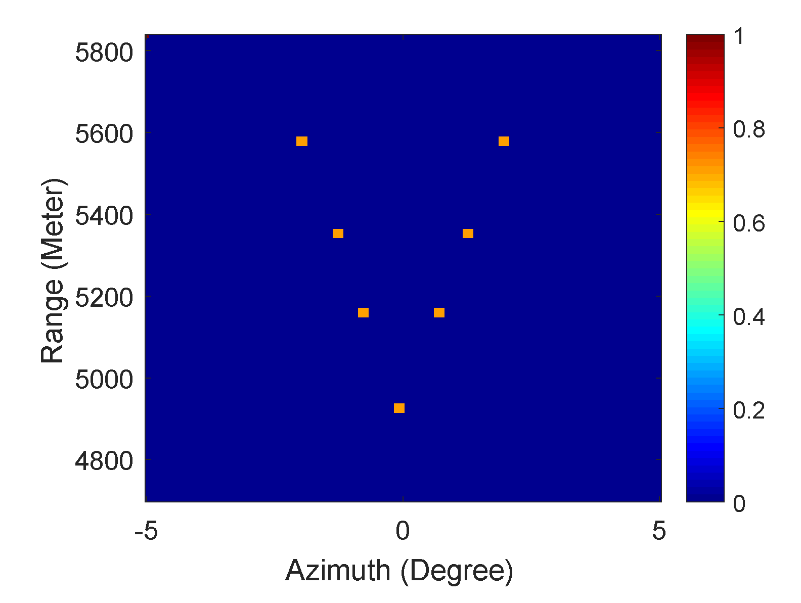
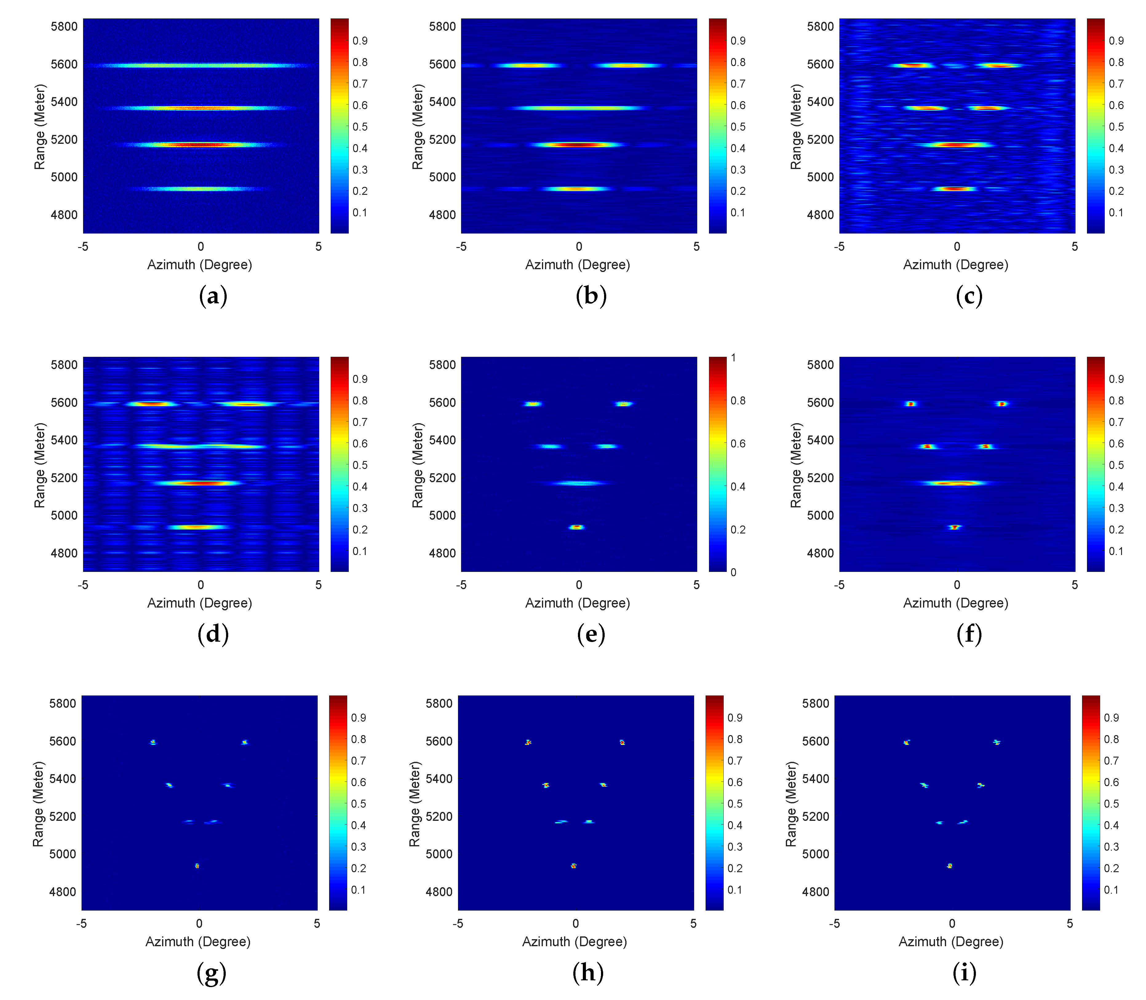
For the simulation, the original scene consisted of three groups of adjacent targets at distances of 5600, 5360, and 5160 m, as well as one island target at a distance of 4930 m, as shown in Figure 2. The antenna pattern was a $sin{c}^2$ function, defined as $\mathrm{sinc}\left(x\right)=sin\left(\pi x\right)/\left(\pi x\right)$, with beam width of 3.5°. Therefore, according to the Rayleigh criterion, the minimum distinguishable distances at the range bin of adjacent targets were $342.08$, $327.42$, and $315.21$ m, respectively. The radar worked in X-band, the scanning region was $\pm 5^{\circ }$, and the scanning speed was ${50}^{\circ }/\mathrm{s}$.

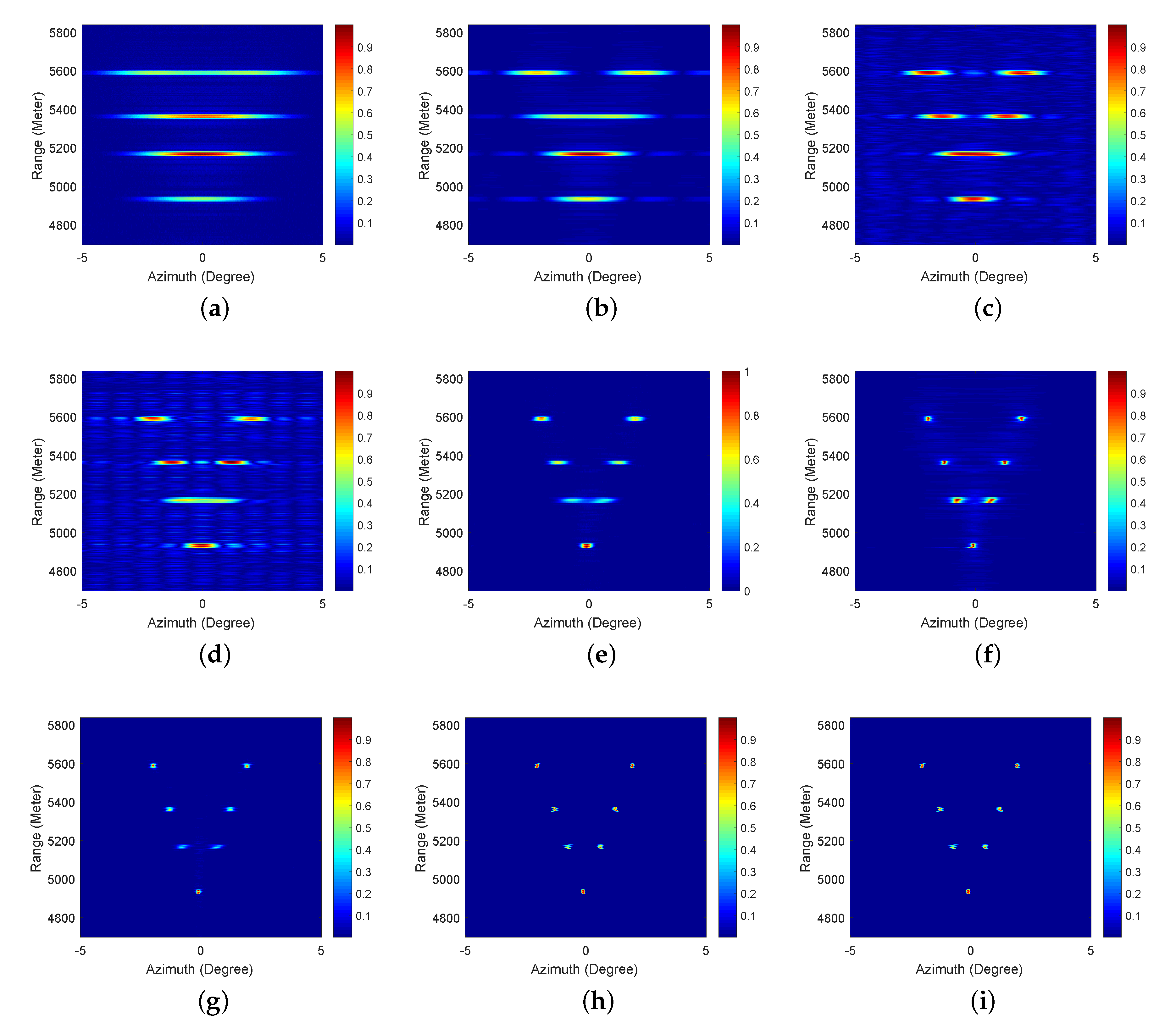
The simulation results are shown in Figure 3. From the prior information, we know that the intervals of adjacent targets were $351.86$, $187.10$, and $108.07$ m, respectively. They are undistinguishable in the real-beam echo. Figure 3a is the real beam echo polluted by white Gaussian white noise (GWN), with signal-to-noise ratio (SNR) of 20 dB, where the SNR is defined as

$$SNR=20{log}_{10}{\displaystyle \frac{{∥\mathit{f}∥}_2^2}{{∥\mathit{y}-\mathit{H}\mathit{f}∥}_2^2}}.$$

(30)

It can be seen that all the adjacent targets could not be distinguished. Figure 3b–i are the results processed by different methods. From the results, WF only could distinguish adjacent targets at 5600 m, with limited improvement in resolution. TSVD and REGU achieved limited resolution improvement. Although adjacent targets at 5600 and 5360 m could be distinguished, the targets at 5160 m could not be distinguished, as shown by Figure 3c,d. From Figure 3e,f, we can see that ML and IAA achieved better resolution improvement than WF, TSVD, and REGU; however, their performance was not as good as SFMM, SBA, and the proposed method. It is obvious that SFMM, SBA, and the proposed method can evidently improve the resolution, as shown by Figure 3g–i. All adjacent targets are distinguished, and the noise is suppressed. Comparing Figure 3i with Figure 3h, it can be seen that the proposed method had almost no performance loss compared to traditional SBA, as it is difficult to discern the differences between them.

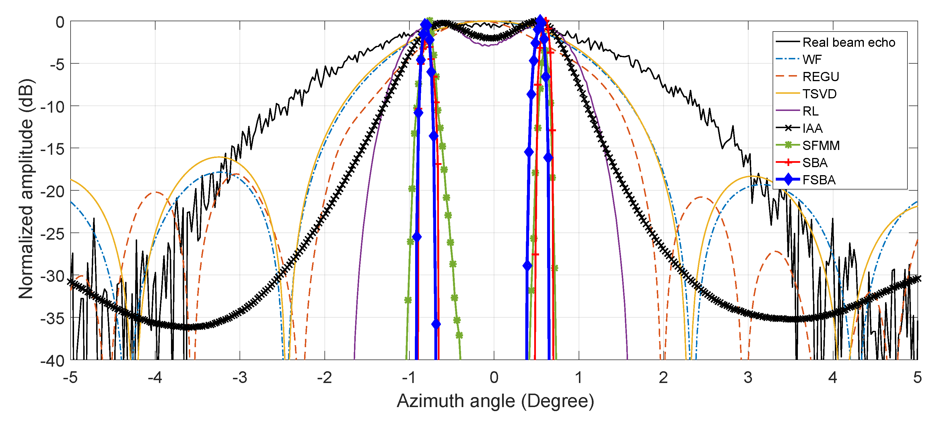
The profiles of the adjacent targets at 5160 m are shown in Figure 4. From the profiles, it is obvious that SFMM, SBA, and FSBA can improve the azimuth resolution better than the other methods. Adjacent targets are completely distinguished and the noise is also suppressed. As for SBA and FSBA, it can be seen that their profiles basically coincide.

In addition, the mean square error (MSE), beam sharpening ratio (BSR), and image entropy were utilized to quantitatively analyze the performances of the different algorithms. The MSE is used to measure the similarity between the processing result and the original scene, which is defined as

$$MSE={\displaystyle \frac{1}{MN}}{∥\widehat{\mathit{\sigma }}-\mathit{\sigma }∥}_2^2.$$

(31)

The BSR is defined as the ratio of beam width before and after processing of a single target, which is used to measure beam sharpening performance. According to the principle of minimum entropy, the image entropy can be used to measure the clarity of an image, as the entropy increases with the increase of image blurring level [44]. The results are shown in

Table 1. Performance of simulation with SNR of 20 dB.

Method	MSE	BSR	Entropy
WF	62.12 × 10${}^{-4}$	1.64	3.81
REGU	74.33 × 10${}^{-4}$	2.41	4.73
TSVD	58.86 × 10${}^{-4}$	2.98	5.14
RL	4.71e × 10${}^{-4}$	10.76	1.83
IAA	6.11 × 10${}^{-4}$	14	3.13
SFMM	4.09 × 10${}^{-4}$	25	0.81
SBA	4.08 × 10${}^{-4}$	25	0.81
FSBA	4.09 × 10${}^{-4}$	25	0.82

.

As can be seen from the table, the MSEs of the processing results of SFMM, SBA, and FSBA were very similar, and much smaller than those of the other methods, which shows that the processing results of these three methods were closer to the original scene. SFMM, SBA, and FSBA achieved the same beam sharpening ability, also far better than the other methods, which is conducive to distinguishing adjacent targets. In addition, the image entropies of the processing results of SFMM, SBA, and FSBA were far less than those of the other methods, which indicates that the quality of their processing results was higher than that of other methods. In conclusion, SFMM, SBA, and FSBA had similar performance, being better than WF, REGU, TSVD, RL, and IAA. As for SFMM, SBA, and FSBA, their performance difference is mainly reflected in computing time. The computing time was tested on the hardware platform; the results are given in the following subsection.

Then, in order to verify the performance of resolution improvement at low SNR, we repeated above simulation with SNR = 10 dB. The simulation results are shown in Figure 5. It can be seen that, under the conditions of low SNR, WF, REGU, TSVD, RL, and IAA could not distinguish adjacent targets at 5160 m. SFMM, SBA and FSBA still had good resolution ability, and all adjacent targets are clearly distinguishable. Similarly, the profiles of the adjacent targets at 5160 m are shown in Figure 6. It can be clearly seen that SFMM, SBA, and FSBA could distinguish adjacent targets, while the other methods could not. The relevant performance indices are shown in

Table 2. Performance of simulation with SNR of 10 dB.

Method	MSE	BSR	Entropy
WF	65.60 × 10${}^{-4}$	1.67	4.18
REGU	75.76 × 10${}^{-4}$	2.12	5.57
TSVD	89.94 × 10${}^{-4}$	1.92	5.48
RL	15.78 × 10${}^{-4}$	7.36	3.55
IAA	20.55 × 10${}^{-4}$	12.72	2.34
SFMM	5.48 × 10${}^{-4}$	24	1.13
SBA	5.12 × 10${}^{-4}$	24	1.14
FSBA	5.98 × 10${}^{-4}$	24	1.16

. From the view of MSE, SBA, and image entropy, we obtained almost the same conclusions as those under the condition of high SNR.

The simulations have demonstrated the superior performance of the proposed FSBA. Having said that, some small approximations have been made in the acceleration process. In the condition of high SNR, these approximations hardly affect the performance of the algorithm. As shown in Figure 3 and Table 1, the results of FSBA and SBA are almost the same. In the condition of low SNR, strong noise will have a slight impact on the performance. From Figure 5 and Table 2, the results of FSBA and SBA are different in MSE and entropy, but these differences are very small and acceptable.

4.2. Real Data Processing

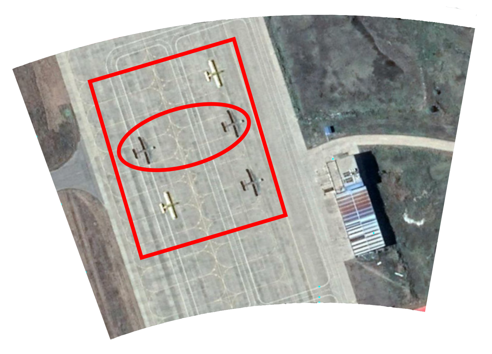
Next, airborne data was processed to verify the performance of the proposed FSBA in practice. In this experiment, a X-band radar was mounted on a transport plane. The beam width was 5.1° and the scanning range was $-{20}^{\circ }$–${10}^{\circ }$.

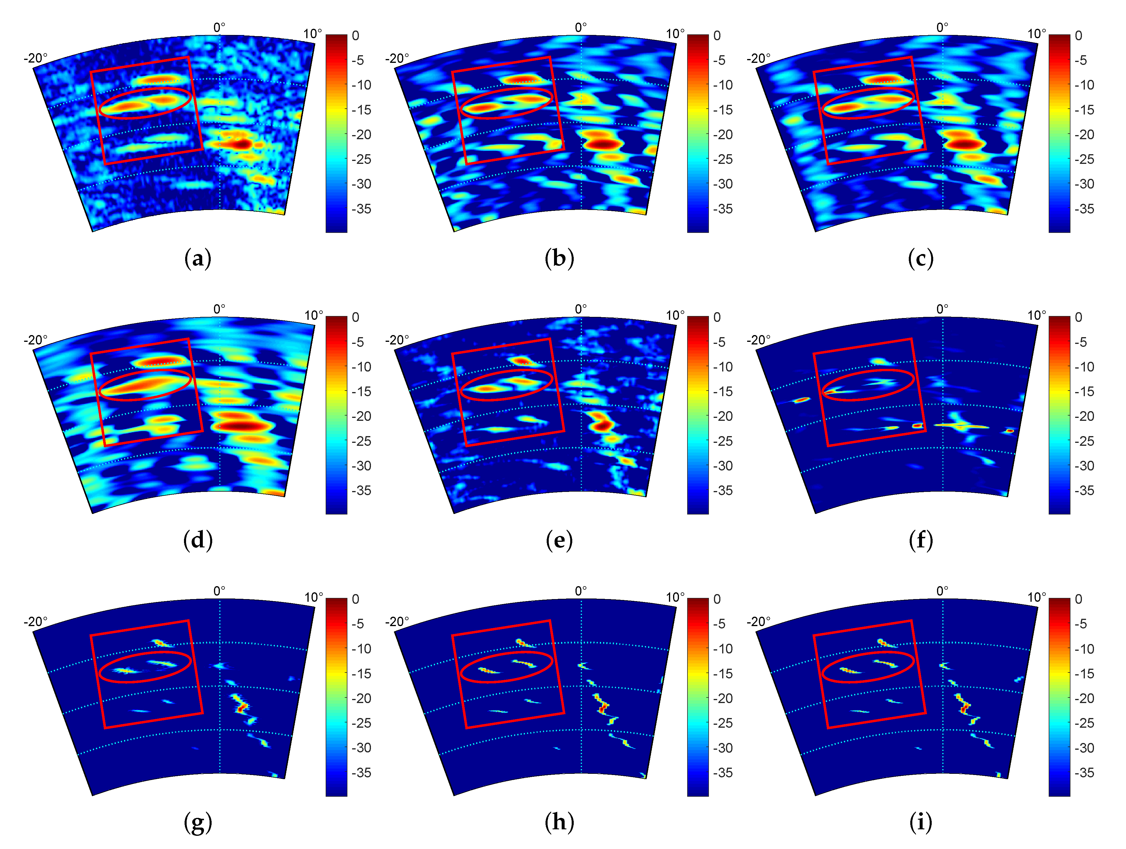
The optical scene, which is shown in Figure 7, was captured from Google earth. It can be seen that the original scene is an airport runway with five co-operative airplanes (marked by the red rectangle). Furthermore, the red circle covers two adjacent airplanes. After antenna scanning, pulse compression, and range walk correction, the real beam echo with low resolution is shown in Figure 8a. In Figure 8a, we cannot distinguish the exact number of planes on the runway. For the real data, the noise is also assumed as GWN and the SNR is defined in Equation (30). Figure 8b–d show that the WF, REGU, and TSVD methods achieved poor resolution improvement and noise suppression. RL and IAA can further improve the resolution, but have limited performance in noise suppression, as shown by Figure 8e,f; in particular, false targets appear in the IAA result, which makes it impossible to determine the number and location of real targets. Figure 8g–i are the processing results of SFMM, SBA, and FSBA, respectively. It can be seen that they have higher resolution and that not only adjacent planes are distinguished, but also the noise is greatly suppressed. Therefore, we can clearly see that the target area has five strong points; that is, the locations of the real targets. Comparing Figure 8h,i, it can be seen that FSBA and SBA had almost the same performance; that is to say, after acceleration, the performance of the SBA had almost no degradation.

The profiles of adjacent airplanes are plotted in Figure 9. It is obvious that SFMM, SBA, and FSBA had a better processing effect than the other methods. Not only are the two targets clearly distinguished, but the noise is also greatly suppressed. For SBA and FSBA, the profiles of their processing results are almost overlapped, which also proves that, after acceleration, the performance of the algorithm has almost no degradation.

In order to quantitatively evaluate the performance of different algorithms, the BSR and entropy are shown in

Table 3. Performance of real data processing.

Algorithm	BSR	Entropy	PSLR (dB)
WF	1.63	4.76	5.51
REGU	1.56	4.67	12.76
TSVD	1.22	5.19	11.37
RL	4.07	3.42	17.08
IAA	4.57	2.16	14.89
SFMM	13.98	1.13	29.96
SBA	14.16	1.12	31.37
FSBA	14.16	1.14	31.36

. Furthermore, the peak side lobe ratio (PSLR) was used to measure the side lobe suppression ability, which is defined as

$$PSLR=20{log}_{10}\frac{A_f}{A_{sl}},$$

(32)

where $A_f$ denotes the signal amplitude and $A_{sl}$ denotes the side-lobe amplitude. From the table, we can see that SFMM, SBA, and the proposed FSBA had better performance in beam sharpening and side lobe suppression than the other methods. Additionally, the entropy of their processing results was smaller than that of the other methods.

It should be noted that, for the processing of real data, it can be seen that although SBA and FSBA can effectively improve the resolution and suppress the noise, they cannot completely separate the target from the noise, and the processing performance is not as good as that with the simulated data. This is due to the assumption of ideal GWN in the simulation; the real world experiment highlights the pitfalls of assuming idealistic noise and clutter sources.

4.3. Assessment of Computing Time

We used the TMS320c6678 chip to test the real-time ability of the proposed FSBA. The main frequency was 1 GHz and the memory was 2 GB. Under this hardware condition, we first give the approximate maximum echo dimension allowed for each algorithm, as shown in

Table 4. Approximate maximum echo dimension allowed for each algorithm.

Algorithms	WF	REGU	TSVD	RL
Dimension	$1800\times 2000$	$220\times 400$	$800\times 400$	$2000\times 1000$
Algorithms	IAA	SFMM	SBA	FSBA
Dimension	$800\times 400$	$800\times 800$	$400\times 400$	$1000\times 2000$

. It can be seen that the maximum echo dimension allowed for FSBA is much larger than other methods except WF and RL. Although the maximum echo dimension allowed for RL and FSBA seems similar, but for airborne radar data, usually we can process each range bin data in turn, and the difficulty of processing depends on the number of azimuth points. That is, the more azimuth data points, the more difficult it is to process. Therefore, the performance of the proposed FSBA to process large-scale data is higher than RL. The maximum data dimension allowed for WF is larger than FSBA, but its resolution improvement is extremely limited.

For above experiments, the dimension of data is $219\times 400$. Based on the hardware platform, the computing times of the different algorithms are listed in

Table 5. Computing time of echo with dimension 219 × 400.

Algorithms	WF	REGU	TSVD	RL	IAA	SFMM	SBA	FSBA
Computing time (s)	0.08	14.02	5.12	0.12	4.11	2.19	11.24	0.22

. The results show that the computing time of the proposed FSBA is much less than that of other methods, except for WF and RL. Although the computing time of WF and RL was less than that of FSBA, it can be seen, from the above experiments, that the performance of WF and RL for resolution improvement was not as good as that of FSBA. Furthermore, the computing time of FSBA can meet real-time requirements. Although SFMM, SBA and FSBA can provide similar results, it is obvious that the computing time of FSBA is much less than SBA and SFMM. In particular, the proposed FSBA only needs about $0.22 \mathrm{s}$ to complete processing, while the traditional SBA needs about $11.24 \mathrm{s}$ and SFMM needs $2.19 \mathrm{s}$. It can be found that the computational efficiency of the proposed FSBA is about 51 times that of SBA and 10 times that of SFMM. As for REGU, TSVD and IAA, their performance of resolution improvement is not as good as that of FSBA, and their computational efficiency is also lower than FSBA. In general, FBSA can perfectly meet the needs of airborne radar real-time resolution improvement in practical applications.

Because the proposed FSBA is accelerated by avoiding matrix inversion, the larger the dimension of echo, the greater the advantage in computational efficiency. To verify this conclusion, the computing time of different algorithms for processing larger dimension echo ($400\times 400$) is shown in

Table 6. Computing time of echo with dimension $400\times 400$.

Algorithms	WF	REGU	TSVD	RL	IAA	SFMM	SBA	FSBA
Computing time (s)	0.15	25.607	9.35	0.22	7.51	6.12	31.53	0.41

. The computing time of the proposed FSBA is also much less than that of other methods, except for WF and RL. In particular, we can obtain that the computational efficiency of the proposed FSBA is about 77 times that of SBA and 14 times that of SFMM.

5. Conclusions

In this paper, we proposed the FSBA to solve the problem of low azimuth resolution in airborne radar imaging. We first transformed the problem of azimuth resolution improvement into an $L_1$ regularization problem. Then, according to the Toeplitz property of the measurement matrix in traditional SBA when solving the $L_1$ regularization problem, we use GS representation to solve the linear equations quickly, skillfully avoiding the matrix inversion operation used in traditional SBA. The proposed method can not only effectively improve the azimuth resolution, but also greatly reduce the computational complexity, which significantly improves the real-time imaging ability.

Through both simulated and real data processing experiments, we demonstrated that the proposed FSBA can greatly improve the resolution, compared with traditional methods, which makes the gray distribution of processing results more uniform and the overall quality better. More importantly, compared with the traditional SBA, the proposed FSBA has almost no performance degradation and its results are almost the same.

Furthermore, the results of hardware test show that the computational efficiency of the proposed FSBA is about 51 times that of SBA and 10 times that of SFMM for echo with $219\times 400$ dimension; for the echo with dimensions of $400\times 400$, the computational efficiency of the proposed FSBA is about 77 times of SBA and 14 times of SFMM, proving that the larger the dimension of the echo, the greater the advantage in computing efficiency.

References

- Uttam, S.; Goodman, N.A. Superresolution of coherent sources in real-beam data. IEEE Trans. Aerosp. Electron. Syst. 2010, 46, 1557–1566. [Google Scholar] [CrossRef]
- Zhang, Y.; Mao, D.; Zhang, Q. Airborne forward-looking radar superresolution imaging using iterative adaptive approach. IEEE J. Sel. Top. Appl. Earth Obs. Remote. Sens. 2019, 12, 2044–2054. [Google Scholar] [CrossRef]
- Li, Z.; Li, S.; Liu, Z. Bistatic Forward-Looking SAR MP-DPCA Method for Space–Time Extension Clutter Suppression. IEEE Trans. Geosci. Remote. Sens. 2020. [Google Scholar] [CrossRef]
- Dropkin, H.; Ly, C. Superresolution for scanning antenna. In Proceedings of the 1997 IEEE National Radar Conference, Ann Arbor, MI, USA, 13 May 1997; pp. 306–308. [Google Scholar]
- Liu, G.; Yang, K.; Sykora, B. Range and azimuth resolution enhancement for 94 GHz real-beam radar. In Proceedings of the XII International Society for Optics and Photonics, Radar, Sensor Technology, Orlando, FL, USA, 15 April 2008; SPIE: Bellingham, WA, USA, 2008; Volume 6947, pp. 1–6. [Google Scholar]
- Zhang, Y.; Jakobsson, A.; Yin, Z.; Huang, Y.; Yang, J. Wideband sparse reconstruction for scanning radar. IEEE Trans. Geosci. Remote. Sens. 2018, 99, 1–14. [Google Scholar] [CrossRef]
- Cruz, C.; Mehta, R.; Katkovnik, V. Single image super-resolution based on Wiener filter in similarity domain. IEEE Trans. Image Process. 2017, 27, 1376–1389. [Google Scholar] [CrossRef]
- Doğu, S.; Akıncı, M.N.; Çayören, M.; Akduman, I. Truncated singular value decomposition for through-the-wall microwave imaging application. IET Microwaves Antennas Propag. 2019, 14, 260–267. [Google Scholar] [CrossRef]
- Kang, M.S.; Kim, K.T. Compressive sensing based SAR imaging and autofocus using improved Tikhonov regularization. IEEE Sensors J. 2019, 19, 5529–5540. [Google Scholar] [CrossRef]
- Campbell, J.F.; Lin, B.; Nehrir, A.R. Super-resolution technique for CW lidar using Fourier transform reordering and Richardson–Lucy deconvolution. Opt. Lett. 2014, 39, 6981–6984. [Google Scholar] [CrossRef]
- Raju, C.; Reddy, T.S. MST radar signal processing using iterative adaptive approach. Geosci. Lett. 2018, 5, 1–10. [Google Scholar]
- Zheng, Y.; Wu, F.; Shim, H.J. Sparse Unmixing for Hyperspectral Image with Nonlocal Low-Rank Prior. Remote Sens. 2019, 11, 2897. [Google Scholar]
- Ghasrodashti, E.; Karami, A.; Heylen, R. Spatial resolution enhancement of hyperspectral images using spectral unmixing and bayesian sparse representation. Remote Sens. 2017, 9, 541. [Google Scholar] [CrossRef] [Green Version]
- Zhang, Y.; Zhang, Q.; Li, C. Sea-Surface Target Angular Superresolution in Forward-Looking Radar Imaging Based on Maximum A Posteriori Algorithm. IEEE J. Sel. Top. Appl. Earth Obs. Remote. Sens. 2019, 12, 2822–2834. [Google Scholar] [CrossRef]
- Candes, E.J.; Wakin, M.B.; Boyd, S.P. Enhancing sparsity by reweighted L1 minimization. J. Fourier Anal. Appl. 2007, 14, 877–905. [Google Scholar] [CrossRef]
- Zhang, Q.; Zhang, Y.; Huang, Y.; Zhang, Y. Azimuth superresolution of forward-looking radar imaging which relies on linearized bregman. IEEE J. Sel. Top. Appl. Earth Obs. Remote. Sens. 2019, 12, 2032–2043. [Google Scholar]
- Osher, S.; Goldstein, T. The split bregman method for L1 regularized problems. SIAM J. Imaging Sci. 2009, 2, 323–343. [Google Scholar]
- Cai, J.F.; Osher, S.; Shen, Z. Split bregman methods and frame based image restoration. Siam J. Multiscale Model. Simul. 2009, 8, 337–369. [Google Scholar] [CrossRef]
- Zhang, Q.; Zhang, Y.; Mao, D. A bayesian superresolution method for forward-looking scanning radar imaging based on split bregman. In Proceedings of the IGARSS 2018-2018 IEEE International Geoscience and Remote Sensing Symposium, Valencia, Spain, 27 July 2018; pp. 5135–5138. [Google Scholar]
- Jazayeri, S.; Kazemi, N.; Kruse, S. Sparse blind deconvolution of ground penetrating radar data. IEEE Trans. Geosci. Remote. Sens. 2019, 57, 3703–3712. [Google Scholar] [CrossRef]
- Smith, D.S.; Gore, J.C.; Yankeelov, T.E.; Welch, E.B. Real-time compressive sensing MRI reconstruction using GPU computing and split bregman methods. Int. J. Biomed. Imaging 2012, 2012, 864827. [Google Scholar]
- Plonka, G.; Ma, J. Curvelet-wavelet regularized split Bregman iteration for compressed sensing. Int. J. Wavelets Multiresolution Inf. Process. 2011, 9, 79–110. [Google Scholar] [CrossRef] [Green Version]
- Ramani, S.; Fessler, J.A. A splitting-based iterative algorithm for accelerated statistical X-ray CT reconstruction. IEEE Trans. Med Imaging 2011, 31, 677–688. [Google Scholar] [CrossRef] [Green Version]
- Chen, D.; Zhu, S.; Cao, X. X-ray luminescence computed tomography imaging based on X-ray distribution model and adaptively split Bregman method. Biomed. Opt. Express. 2015, 6, 2649–2663. [Google Scholar] [CrossRef] [PubMed] [Green Version]
- Aggarwal, P.; Gupta, A. Accelerated fMRI reconstruction using matrix completion with sparse recovery via split bregman. Neurocomputing 2016, 216, 319–330. [Google Scholar] [CrossRef]
- Beck, A.; Teboulle, M. A fast iterative shrinkage thresholding algorithm for linear inverse problems. Siam J. Imaging Sci. 2009, 2, 183–202. [Google Scholar]
- Zhang, Q.; Zhang, Y.; Huang, Y. Sparse with Fast MM Superresolution Algorithm for Radar Forward-Looking Imaging. IEEE Access 2019, 7, 105247–105257. [Google Scholar]
- Osher, S.; Mao, Y.; Dong, B.; Yin, W. Fast linearized Bregman iteration for compressive sensing and sparse denoising. arXiv 2011, arXiv:1104.0262. [Google Scholar]
- Freund, R.W.; Zha, H. A look-ahead algorithm for the solution of general hankel systems. Numer. Math. 1993, 64, 295–321. [Google Scholar] [CrossRef]
- Zhang, Y.; Yin, Z.; Li, W.; Huang, Y.; Yang, J. Superresolution surface mapping for scanning radar: Inverse filtering based on the fast iterative adaptive approach. IEEE Trans. Geosci. Remote. Sens. 2018, 99, 1–18. [Google Scholar] [CrossRef]
- Glentis, G.O.; Jakobsson, A. Time-recursive IAA spectral estimation. IEEE Signal Process. Lett. 2010, 18, 111–114. [Google Scholar] [CrossRef]
- Kailath, T. Some new algorithms for recursive estimation in constant linear systems. Inf. Theory IEEE Trans. 1974, 19, 750–760. [Google Scholar]
- Bitmead, R.R.; Anderson, B.D.O. Asymptotically fast solution of toeplitz and related systems of linear equations. Linear Algebra Appl. 1980, 34, 103–116. [Google Scholar] [CrossRef] [Green Version]
- Glentis, G.O.; Jakobsson, A. Efficient implementation of iterative adaptive approach spectral estimation techniques. IEEE Trans. Signal Process. 2011, 59, 4154–4167. [Google Scholar] [CrossRef]
- Karlsson, J.; Rowe, W.; Xu, L.; Glentis, G.O.; Jian, L. Fast missing-data IAA with application to notched spectrum SAR. IEEE Trans. Aerosp. Electron. Syst. 2014, 50, 959–971. [Google Scholar] [CrossRef]
- Sidky, E.; Pan, X. Image reconstruction in circular cone-beam computed tomography by constrained, total variation minimization. Phys. Med. Biol. 2008, 53, 4777. [Google Scholar] [PubMed] [Green Version]
- Guangcan, L.; Zhouchen, L.; Shuicheng, Y.; Ju, S.; Yong, Y.; Yi, M. Robust recovery of subspace structures by low-rank representation. IEEE Trans. Pattern Anal. Mach. Intell. 2013, 35, 171–184. [Google Scholar]
- Getreuer, P.; Fatemi, R. Rudin-osher-fatemi total variation denoising using split bregman. Image Process. Line 2012, 2, 74–95. [Google Scholar] [CrossRef]
- Lee, U. Spectral Analysis of Signals; Prentice-Hall: Upper Saddle River, NJ, USA, 2005. [Google Scholar]
- Glentis, G.O.; Jakobsson, A. Superfast approximative implementation of the iaa spectral estimate. IEEE Trans. Signal Process. 2011, 60, 472–478. [Google Scholar] [CrossRef] [Green Version]
- Jensen, J.R.; Glentis, G.O.; Christensen, M.G. Fast LCMV-based methods for fundamental frequency estimation. IEEE Trans. Signal Process. 2013, 61, 3159–3172. [Google Scholar] [CrossRef] [Green Version]
- Azadbakht, M.; Fraser, C.; Khoshelham, K. A sparsity-based regularization approach for deconvolution of full-waveform airborne lidar data. Remote. Sens. 2016, 8, 648. [Google Scholar] [CrossRef] [Green Version]
- Zhang, Q.; Zhang, Y. TV-Sparse Super-Resolution Method for Radar Forward-Looking Imaging. IEEE Trans. Geosci. Remote. Sens. 2020. [Google Scholar] [CrossRef]
- Long, T.; Lu, Z.; Ding, Z.; Liu, L. A DBS Doppler centroid estimation algorithm based on entropy minimization. IEEE Trans. Geosci. Remote. Sens. 2011, 49, 3703–3712. [Google Scholar] [CrossRef]
Figure 1.
Signal processing scheme.
Figure 2.
Original scene of simulation.
Figure 3.
Results of simulation with signal-to-noise ratio (SNR) of 20 dB: (a) Real beam echo; (b) Wiener filtering (WF); (c) Tikhonov regularization (REGU); (d) truncated singular value decomposition (TSVD); (e) Richardson–Lucy (RL); (f) iterative adaptive approach (IAA); (g) sparse with fast Majorization-Minimization (SFMM); (h) Split Bregman algorithm (SBA); and (i) fast split Bregman algorithm (FSBA).
Figure 4.
Profiles of adjacent targets with SNR of 20 dB.
Figure 5.
Results of simulation with SNR of 10 dB: (a) Real beam echo; (b) WF; (c) REGU; (d) TSVD; (e) RL; (f) IAA; (g) SFMM; (h) SBA; and (i) FSBA.
Figure 6.
Profiles of adjacent targets with SNR of 10 dB.
Figure 7.
Optical scene of experiment.
Figure 8.
Results of airport data: (a) Real beam echo; (b) WF; (c) REGU; (d) TSVD; (e) RL; (f) IAA; (g) SFMM; (h) SBA; and (i) FSBA.
Figure 9.
Profiles of local regions in Figure 8.