Non-Destructive Early Detection and Quantitative Severity Stage Classification of Tomato Chlorosis Virus (ToCV) Infection in Young Tomato Plants Using Vis–NIR Spectroscopy

Abstract

Tomato chlorosis virus (ToCV) is a serious, emerging tomato pathogen that has a significant impact on the quality and quantity of tomato production worldwide. Detecting ToCV via means of spectral measurements in an early pre-symptomatic stage offers an alternative to the existing laboratory methods, leading to better disease management in the field. In this study, leaf spectra from healthy and diseased leaves were measured with a spectrometer. The diseased leaves were subjected to RT-qPCR for the detection and quantification of the titer of ToCV. Neighborhood component analysis (NCA) algorithm was employed for the feature selection of the effective wavelengths and the most important vegetation indices out of the 24 that were tested. Two machine learning methods, namely XY-fusion network (XY-F) and multilayer perceptron with automated relevance determination (MLP–ARD), were employed for the estimation of the disease existence and viral load in the tomato leaves. The results showed that before outlier elimination, the MLP–ARD classifier generally outperformed the XY-F network with an overall accuracy of 92.1% against 88.3% for the XY-F. Outlier elimination contributed to the performance of the classifiers as the overall accuracy for both XY-F and MLP–ARD reached 100%.

1. Introduction

Agriculture plays a significant role in the economic domain worldwide. The continuously increasing demand for food due to the increase of the global population has triggered the evolution of novel agro-technology methods in the sector of precision agriculture (PA) in order to optimize the productivity and reduce the agricultural waste and the production loss that is caused by biotic and abiotic factors [1,2].

Plant diseases constitute a great threat for the agricultural sector in a worldwide scale, causing significant loss of global production [3]. Diseases in the field and greenhouse conditions are mostly addressed with the use of chemical compounds if the disease is curable. Although this method could be proven efficient, the cost of pesticides is large and the results are questionable. Apart from the economic impact, such methods also have a negative environmental impact [1]. Additionally, in the case of viral diseases, their control is mainly based on preventive measures since it is not possible to cure the infected plants. Thus, it is necessary that there be targeted early detection for the efficient management of such diseases. For these purpose, preventive means and post infection methods are employed, aiming to minimize the extent of the impact of disease damages. Compared to destructive methods, these approaches are noninvasive, since they can be applied on the same plants over time [4]. These approaches can yield useful data from the spectral bands outside the visual spectrum, enhancing crop monitoring potential [5,6].

The tomato yellows disease (TYD) is a serious tomato disease that causes leaf deterioration through yellowing and interveinal chlorosis and leads to important yield losses of the affected crops worldwide [7,8]. Two pathogens of the genus Crinivirus are implicated in this disease: tomato chlorosis virus (ToCV) and tomato infectious chlorosis virus (TICV) [8]. At the worldwide level, ToCV prevails over TICV [9]. Tomato yield is negatively affected by ToCV infection, although tomato fruits are not directly affected, due to loss of photosynthetic area, which causes smaller and reduced number of fruits [10]. The virus is semipersistently transmitted by the whitefly species Trialeurodes varopariorum, Bemisia tabaci (MED and MEAM1) and Trialeurodes abutilonea [10]. Methods to reduce the spread of ToCV in the field are limited to controlling the whitefly population, as there are no commercially available resistant or tolerant tomato varieties to date, and management of the virus sources [9].

Visible symptoms typically appear at least 2–3 weeks after virus inoculation in healthy tomato plants. Spectroscopy methods are employed for preventive screenings, which are non-destructive and could potentially detect the pathogen long before the appearance of symptoms. Examples of spectroscopy methods employed for prevented screening have been presented by Gold et al. [11], Fernández et al. [12] and Herrmann et al. [13]. Thus, removing infected plants before the virus transmission in neighboring plants or crops susceptible to the virus could be of vital importance for the growers in retaining the production.

The conventional laboratory methods and techniques that are used for the detection of ToCV infection include the serological technique of ELISA, which is generally considered an efficient method for criniviruses such as ToCV [14,15,16], and real-time RT-PCR assay [14,17].

Spectroscopy techniques, such as fluorescence, Vis–NIR spectroscopy [11] and hyperspectral imaging [18], among others, are non-destructive methods for the study of the leaves’ spectral responses under any biotic and abiotic stresses that they are subjected to [19,20]. Such methods have been successfully used for the detection and the diagnosis of plant diseases and weeds both on laboratory and field levels and in an early stage of the epidemic [13,21,22,23,24,25,26] or in a later stage for precise targeting of herbicides and pesticides [27,28,29,30]. When spectroscopy methods are applied, differences between the healthy and the infected areas of the leaves can be assessed by the study of the shifting of visible and NIR curves. The visible spectrum area has typically lower reflectance due to absorption by leaf pigments, mostly chlorophyll, caretonoids and anthocyanins [31]. Reflectance in the NIR region depends on the leaf cellular structure [32]. Such differences in the way leaf pigments and structure interact with electromagnetic radiation can be detected by specialized spectrometry equipment in order to discriminate between healthy and infected plants [28], as plant diseases affect the leaf pigments, cellular structure and metabolic activity and even the leaf texture characteristics. In this paper, leaf reflectance in the Vis–NIR spectrum is employed in order to identify and quantify ToCV in young tomato plants.

The aim of this paper is the development of an algorithm for nondestructive detection of a possible ToCV infection in young tomato plants, taking also into account the intensity level of the infection using the spectral signatures that are collected by a portable Vis–NIR spectrometer. The intensity levels of the virus infection that was examined are based on the quantitative virus concentration of the plants and are subject to the detection of ToCV before there is any visible symptom on the plants’ leaves. For the detection of the pathogen, the machine learning classification methods of XY-fusion networks (XY-F) and multilayer perceptron with automatic relevance determination (MLP–ARD) artificial neural networks (ANN) were employed and compared to each other for their accuracy, using effective wavelengths and vegetation indices that were selected by neighborhood components analysis (NCA) algorithm.

2. Materials and Methods

2.1. Plant Material and Growth Conditions

Biologically untreated tomato plants (Solanum lycopersicum L. hybrid Belladonna) were placed in a growth chamber with controlled environment. The temperature was set in a 23/25 °C day/night cycle, and the mean relative humidity was 70 ± 10%. Illumination was provided by artificial fluorescent lighting (Philips 32-Watt T8 4 ft Plant and Aquarium) under a 16 h photoperiod regime per day. The lamps were placed 65 cm above the plants with a mean photosynthetic photon flux density (PPFD) of 410 μmol·m⁻²·s⁻¹. Commercial enriched brown potting peat soil (Agricult^®) mixed with vermiculite in a 3:1 ratio was used with a composition of 70% blond peat, 30% black peat and 1.5 kg of PG-Mix (12–14–24), with a pH of 5.6–6.4.

2.2. ToCV Infection and Quantitative Analysis

A total of 156 tomato plants were used as the experimental material, of which 132 were used for virus infection, and the remaining 24 served as negative controls. The isolate ToCV/Rh1835 (GenBank accession number HG380092) originated from a greenhouse in Rhodes Island (Greece), and it was maintained in an insect-proof cage by serial passages onto tomato plants (Solanum lycopersicum hybrid Belladonna) in the Laboratory of Plant Pathology (Aristotle University of Thessaloniki, Greece) using the whitefly vector Bemisia tabaci MED.

ToCV-infected tomato plants (hybrid Belladonna) were used as viral sources 4 weeks post inoculation (wpi). Twelve groups of 40 adult whiteflies were given a 48-h acquisition access period (AAP) on source plants, and a 72-h inoculation access period (IAP) was followed in order to achieve maximum transmission efficiency. Then, clip cages were removed and all plants were sprayed with the insecticide imidacloprid. Clip-cages are useful experimental tools for gathering and transferring small insects, such as whiteflies, to leaves when aiming to study various biological parameters [33]. Plants were transferred to the chamber where they were grown for approximately two weeks (until the appearance of interveinal yellowing symptoms induced by ToCV). During this period no visible signs of leaf senescence was observed in the plant material that was used.

Finally, the tomato plants were taken to the laboratory, and the first true leaf in which the whiteflies were fed and transmitted the virus was treated by removing lingering dust and dirt for spectral signature acquisition. Eleven spectral measurements were taken during this two week period. The first three measurements occurred within a two-day time interval, and after that there was a measurement every day until the end of the experiment. After the optical measurements, approximately 0.2 g of the leaf was cut off the plant and stored at −80 °C until it was processed. Total RNA was extracted from all leaves from both negative control treatments and infected plants and subjected to RT-qPCR for detection and quantitation of ToCV in infected tissues according to the protocols described by Orfanidou et al. [34].

2.3. Optical Measurements

For each optical measurement that was performed during the experiment, 12 infected tomato plants were randomly picked from the growth chamber and carried to the laboratory. The measurements were carried out using a portable Unispec-SC spectrometer (PP Systems, Inc.). This specific spectral instrument provides robust spectral measurements (reflectance and absorbance) in the visible and near infrared range between 310 nm and 1100 nm with a sampling interval of 3.3 nm and a spectral resolution (FWHM) of less than 10 nm. The leaf spectral signature acquisition was performed through a halogen light source mounted on a leaf clip. A 100% white reference scan was performed before the initial scanning, and it was repeated before each individual measurement. The spectra in the range 310 nm to 399 nm and in the range 1001 nm to 1100 nm at the fringe of the active range of the spectrophotometer showed an excessive noisy pattern and were removed from further analysis.

At least 15 spectral scans were collected from each tomato plant sample, depending on the plant leaf area. The greater the leaf area, the more spectral samples were collected so that there would be a representative sample collection. The negative control plants were scanned three times during the experimental procedure. The first occurred on the first day of the start of the spectral measurements, the second occurred on the sixth day and the last one on the twelfth day.

2.4. Spectral Data Pre-Processing and Feature Selection

It is crucial for the success of the classifiers’ training phase to exclude any excessive non-linearity that is related with noise or any other external effect that is caused either by the spectral measurement instrument sensitivity or the measurement conditions [35]. For this reason, apart from just removing the noisy edges of the spectrometer, as mentioned above, there was further smoothing of the spectral data. Transforming the raw Vis–NIR reflectance data (R) using their transpose logarithm, log(1/R), was used as it was found to be very efficient in the quantification of plant pigments [36,37]. Additionally, the data were mean centered, and finally the Savitzky–Golay smoothing filter [38] was applied, using five supporting points on each edge of the smoothing point and by applying a third-degree polynomial.

Apart from data pre-processing, there was outlier detection in the spectral data, which was decided after performing high-dimensional robust principal component analysis (HR-PCA) as described by Xu et al. [39]. The outlier elimination was performed by iteratively omitting the largest data points from the PCA projection of the principle components that covered at least 80% of the total variance. Both the results of the predictive accuracy before and after the outlier elimination are presented in this paper.

Due to the high dimensionality that the spectral data show, they are not suggested to be used as a model input in statistical and machine learning methods. The problem is mostly related to the limited useful information that these data carry, which in turn lead to lower model performance due to lower variance, as well as the increase of the computational time. Instead, in most cases, dimensionality reduction techniques are used, such as principal component analysis (PCA) or techniques for feature selection. In this study, it was decided to examine the effect of selected vegetation indices (VIs) from the literature (

Table 1. Spectral vegetation indices that were used for feature selection in this study.

Index Abbreviation	Index Name	Index Formula	Reference
NDVI	Normalized Difference Vegetation Index	$\frac{R_{800}-R_{670}}{R_{800}+R_{670}}$	[41]
NSRI	NIR Shoulder Ratio Index	$\frac{R_{890}}{R_{780}}$	[42]
NDRE	Normalized Difference Red Edge	$\frac{R_{790}-R_{720}}{R_{790}+R_{720}}$	[43]
TVI	Triangular Vegetation Index	$0.5\ast \left[120\ast \left(R_{750}-R_{550}\right)-200\ast \left(R_{670}-R_{550}\right)\right]$	[44]
ARI	Anthocyanin Reflectance Index	$\frac{1}{R_{550}}-\frac{1}{R_{700}}$	[45]
CSI1	Carter Stress Index	$\frac{R_{695}}{R_{420}}$	[46]
GM1	Gitelson and Merzylak Index 1	$\frac{R_{750}}{R_{550}}$	[47]
gNDVI	green Normalized Difference Vegetation Index	$\frac{R_{810}-R_{560}}{R_{810}+R_{560}}$	[48]
LCI	Leaf Chlorophyll Index	$\frac{R_{850}-R_{710}}{R_{850}+R_{680}}$	[49]
LIC1	Lichtenhaler Index	$\frac{R_{800}-R_{680}}{R_{800}+R_{680}}$	[50]
MCARI1	Modified Chlorophyll Absorption Ratio Index 1	$1.2\ast \left[2.5\ast \left(R_{800}-R_{670}\right)-1.3\ast \left(R_{800}-R_{550}\right)\right]$	[51]
MCARI2	Modified Chlorophyll Absorption Ratio Index 2	$\frac{1.2\ast \left[2.5\ast \left(R_{800}-R_{670}\right)-1.3\ast \left(R_{800}-R_{550}\right)\right]}{\sqrt{\left[{\left(2\ast R_{800}+1\right)}^2-\left(6\ast R_{800}-5\ast \sqrt{R_{680}}-0.5\right)\right]}}$	[51]
MTVI1	Modified Triangular Vegetation Index 1	$1.2\ast \left[1.2\ast \left(R_{800}-R_{550}\right)-2.5\ast \left(R_{670}-R_{550}\right)\right]$	[51]
MTVI2	Modified Triangular Vegetation Index 2	$\frac{1.5\ast \left[1.2\ast \left(R_{800}-R_{550}\right)-2.5\ast \left(R_{670}-R_{550}\right)\right]}{\sqrt{\left[{\left(2\ast R_{800}+1\right)}^2-\left(6\ast R_{800}-5\ast \sqrt{R_{670}}\right)-0.5\right]}}$	[51]
PSSRa	Pigment Specific Simple Ratio (Chl a)	$\frac{R_{800}}{R_{675}}$	[52]
PSSRb	Pigment Specific Simple Ratio (Chl b)	$\frac{R_{800}}{R_{650}}$	[52]
PSSRc	Pigment Specific Simple Ratio (Carotenoids)	$\frac{R_{800}}{R_{500}}$	[52]
RDVI	Renormalized Difference Vegetation Index	$\frac{R_{800}-R_{670}}{\sqrt{R_{800}+R_{670}}}$	[53]
REIP	Red Edge Inflection Point	$700+40\ast \frac{R_{RE}-R_{700}}{R_{740}-R_{700}}, where R_{RE}=\frac{R_{670}+R_{780}}{2}$	[54]
REIP1	Modified Red Edge Inflection Point	$700+\left(\frac{740}{700}\right)\ast \frac{R_i-R_{700}}{R_{740}-R_{700}}, where R_i=\frac{R_{780}}{R_{670}}$	[55]
SRCHLTOT	Simple Ratio of Total Chlorophyll Content	$\frac{R_{760}}{R_{500}}$	[48]
VOG1	Vogelmann Index 1	$\frac{R_{740}}{R_{720}}$	[56]
VOG2	Vogelmann Index 2	$\frac{R_{734}-R_{747}}{R_{715}-R_{720}}$	[56]
VOG3	Vogelmann Index 3	$\frac{R_{734}-R_{747}}{R_{715}-R_{726}}$	[56]

) on the presymptomatic detection of ToCV infection on young tomato plants [40]. Apart from the VIs, the most effective raw wavelengths were also evaluated for their effect on the disease detection. The effective wavelengths were decided through neighborhood component analysis.

2.5. Feature Selection

Adding many predictors in a model increases its complexity, which may improve the quality of the training process but can have strongly negative impacts on the predictive accuracy. For this reason, the abovementioned VIs, as well as the EWs that were used as features in the classification models were decided by using the neighborhood component analysis (NCA) method, which was based on Yang et al.’s [57] implementation for feature selection of the original Goldberger et al. [58] algorithm.

The NCA method is a feature selection algorithm that learns a low dimensional embedding of the data for kNN classification using a direct gradient-based approach [59]. The quadratic (Mahalanobis) distance metrics are used because they can be represented by the symmetric positive semi-definite matrices. The aim of this algorithm is to find a system for determining the ideal feature distance through a linear transformation of input data to optimize classification in the transformed space. The irrelevant feature weights get reduced to zero, under the leave one out classification scheme. In this paper the feature weights were estimated using the stochastic gradient descent (SGD) solver.

The initial learning rate value was set to 0.1, and the learning rate tuning iteration was set to 20. After 16 iterations, the convergence was accomplished to a learning rate value of 6.4. Optimum lambda regularization hyperparameter (which minimizes the generalization error) was determined after its tuning using five-fold cross-validation and was found to be 0.004. Total subset size that the threshold (θ) above which the most significant features were selected was decided according to Equation (1) [60].

$$\mathsf{\theta }=\mathsf{\tau }·\max \left(w\right)$$

(1)

In this equation, τ denotes the tolerance set at 0.2 [60], and max(w) denotes the maximum value of the updated features weight vector.

2.6. Class Division

The initial division of the tomato samples into the control (healthy) and infected (virus positive) classes was done according to Orfanidou et al. [34], after the quantitative measurement of ToCV on tomato leaves. In their research, Orfanidou et al. [34] define the cycle threshold (Ct) value of 43.3 as a limit for positive ToCV detection. Any value in the Ct range of 30 to 43.5 is considered not detectable, and any higher value belonged to the negative control plants. The class division that reflected the different severity stages of the virus infection and that was used for the classifier training is shown in

Table 2. Class division of tomato plants into healthy (control) and three disease severity stages according to their cycle threshold (Ct) value.

Ct Value	Class Characteristics	Class Label
>43.5	Control—Not infected	1
43.5–30	Very low infection—No symptoms and hardly detectable viral concentration	2
30–25.5	Low to mid infection—No symptoms and detectable viral concentration	3
25.5–20	Mid to high infection—First symptoms	4

. A total of 2984 spectral signatures were collected from the plants. Out of those spectral signatures, 680 belonged to the control treatment, 749 belonged to class 2, 761 to class 3, and the remaining 794 belonged to mid to highly infected leaves (class 4).

2.7. Machine Learning Techniques

The machine learning techniques used in this paper were XY-fused networks and multilayer perceptron with automated relevance determination (MLP–ARD). XY-fused networks [61] are supervised artificial neural networks that are used for classification modelling in a similar way as supervised Kohonen maps. The winning neuron is defined from the fused similarity of the Euclidean distances calculation between the n input feature (x_n) and their respective weights and the target class vector [62]. A graphical representation of the architecture of such a network is shown in Figure 1.

Multilayer perceptron with automated relevance determination (MLP–ARD) neural networks were employed in this study as an alternative to the XY-fusion network. MLPs are feed forward artificial neural networks, which in classification problems map a set of input vectors onto their respective classes. For this study, a fully connected MLP with a three-layer architecture (input layer, hidden layer and output layer) was assigned for the classification of the spectral signatures into the healthy or the intensity of the disease level conditions. The weight correction was performed by the scaled conjugate gradient back propagation algorithm, and the transfer function that were selected were the hyperbolic tangent (tanh) for the interconnections between the input and the hidden layer and the logistic function for the respective interconnections between the hidden and the output layer. The values of the weights were chosen by minimizing the value of the cost function G (Equation (2)):

$$G=-\frac{1}{m}{\displaystyle \sum }_{i=1}^m\left[t_i\log \left(y_i\right)+\left(1-t_i\right)\log \left(1-y_i\right)\right],$$

(2)

where t_i is the target class, y_i is the classifier output, m i ∈ $\mathbb{Z}$ is the number of the training samples and i $\in \mathbb{Z}$ ∈ $\mathbb{Z}$ is the index of a specific sample.

Apart from the first level hyperparameters, the values of which were randomly chosen as priors for the initialization of the MLP classifiers, automatic relevance determination (ARD) was used in this study. In the application of the ARD technique, a new regularization hyperparameter, alpha (α), was introduced for every weight associated with the i input variables in order to determine the relevance of the input data into the model. Evidence maximization was used to infer the regularization parameters, and the inputs with the largest α_i values were not used for further analysis. In the specific algorithm, three additional alpha hyperparameters, including weight classes, were demonstrated; the first was related to the synaptic connection bias, the second to the interconnections between the hidden and the output neurons, and the last one was associated with the connection between the hidden layer bias neuron and the output neurons [63].

A quantification of the influence of the individual features in the model can be derived by the magnitude of L2 regularization norms of the weights and the relevant values of the alpha hyperparameter (α_k) that can be calculated using Equation (3).

$$F\left(W\right)=G+\frac{1}{m}{\displaystyle \sum }_k{a}_k{Ew}_{\mathrm{k}},$$

(3)

where k $\in \mathbb{Z}$, $E{w}_k=\frac{1}{2}\sum w_{kj}^2$, w_j $\in$ ℝ, represents the weights and j weight indicator of the class W_(k).

Both of the classification models that were used for this study had their optimal network architecture hyperparameters, such as the training epoch number and the hidden layer size of the network defined by the means of genetic algorithm (GA) implementation, as described by Ballabio et al. [64], for five different learning rate values. The optimization parameters and their respective values that were set to be optimized are shown in

Table 3. Neural network hyperparameter values that were tested by a genetic algorithm (GA) for the architecture optimization of the classifiers that were used.

Network Hyperparameters	Values
Training Epoch Number	50, 100, 200, 300, 500, 600, 1000
Self Organizing Map (SOM)/Hidden Layer Size	4, 8, 10, 15, 20, 25, 30
Learning Rate	0.001, 0.005, 0.01, 0.02, 0.05

.

For the XY-F network, the optimal architecture was for 200 epochs, a 10 × 10 self organizing map (SOM) layer and a learning rate of 0.005, while for the MLP–ARD network, the respective hyperparameters that were chosen were 500 training epochs, 10 hidden units and a learning rate of 0.005.

All the data analyses and the implementation of the classification methods were carried out using MATLAB software, version 9.5 (R2018b) by Mathworks^® Inc. (Natick, MA, USA).

2.8. Model Evaluation Metrics

Before data analysis, the whole dataset of the spectral signatures was divided into training and testing sets by randomly picking samples from the spectral dataset and by using the ordinary 70–30% scheme for the respective training and testing set divisions. The predictive ability of the trained models were addressed using the confusion matrix from the classifier by which the F1 score and the accuracy were computed, as shown in Equations (6) and (7). In these equations, the notation TP corresponds to the true positive predictions, TN to the true negative, FP to the false positive and FN to the false negative predictions.

$$\mathrm{Recall}=\frac{\mathrm{TP}}{\mathrm{TP}+\mathrm{FN}}$$

(4)

where

$$\mathrm{Precision}=\frac{\mathrm{TP}}{\mathrm{FP}+\mathrm{TP}}$$

(5)

$$\mathrm{F}1 \mathrm{Score}=2·\frac{\mathrm{Recall}·\mathrm{Precision}}{\mathrm{Recall}+\mathrm{Precision}}$$

(6)

$$\mathrm{Accuracy}=\frac{\mathrm{TP}+\mathrm{TN}}{\mathrm{TP}+\mathrm{TN}+\mathrm{FP}+\mathrm{FN}}$$

(7)

Although Accuracy is a widely used evaluation metric in the literature, it also implies balanced class distribution in order to give a trustworthy and robust result. In practice though, this is not always the case, as it is many times more difficult to have balanced class distribution. F1-score can tackle this problem in a better way than accuracy, as it is the weighted average of precision and recall and penalizes extreme values in any class.

3. Results

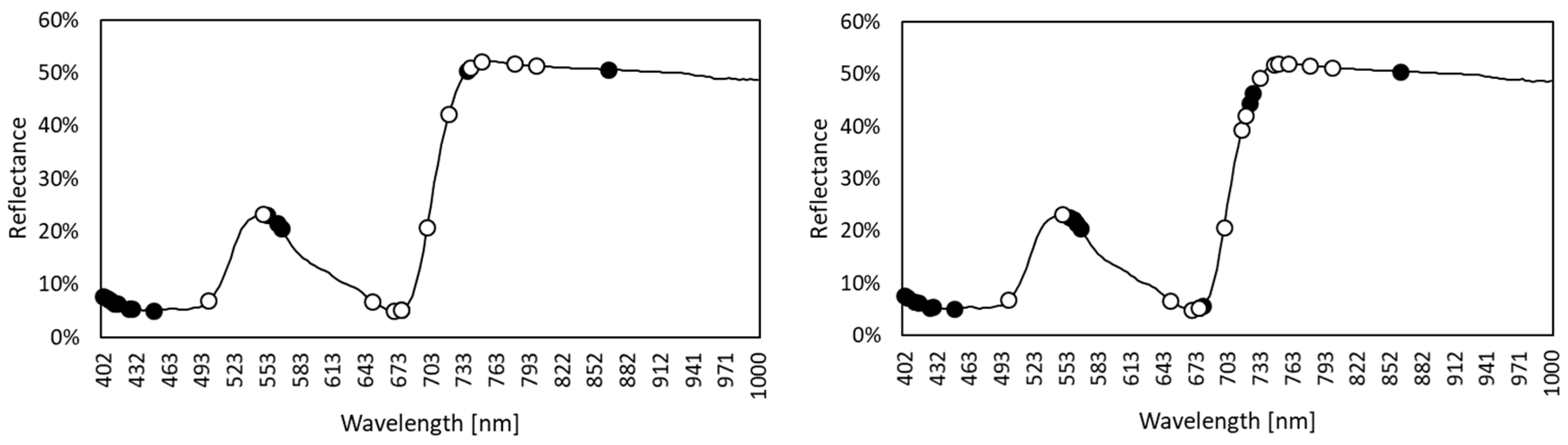
3.1. Spectral Data Overview

Both before and after the outlier elimination it could be concluded that the pattern of the spectral signature was dependent on the disease severity (Figure 2). In both cases it could be seen that there was an inversely proportional attitude for the spectral peaks in the visible and in the near infrared region.

Before the outlier elimination the mean spectral signatures seemed to be closer to each other, in comparison with the data after the outlier elimination, and this could make the classification process more difficult, as it was possible that there would be some overlap between the spectral signatures. A more distinct class division can ensure most of the time a more successful classification [65].

An optical comparison between the graphs in Figure 3 can show that there was almost no influence of the proposed outlier elimination in the visible part of the spectral signature, but in the NIR part, especially after the red edge peak at 750 nm, there was a distinct difference between the different classes. While the data before the outlier elimination showed that in this part of the spectrum it was difficult to differentiate mean spectral response between the class couple 1 and 2 and the class couple 3 and 4, nevertheless, it seemed like after the outlier elimination, the classes became more distinct to each other, with class 1 being on the top and class 2, 3 and 4 following in an order of increasing severity.

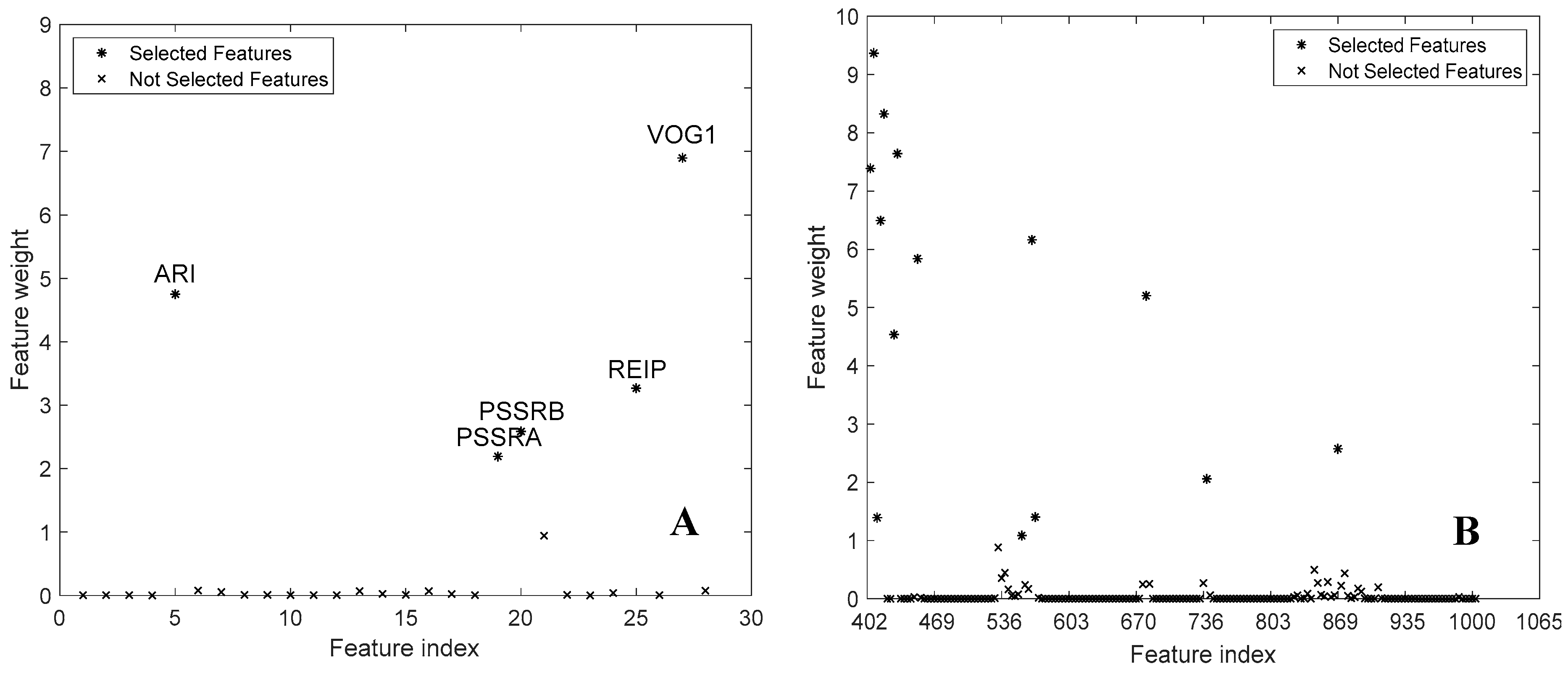
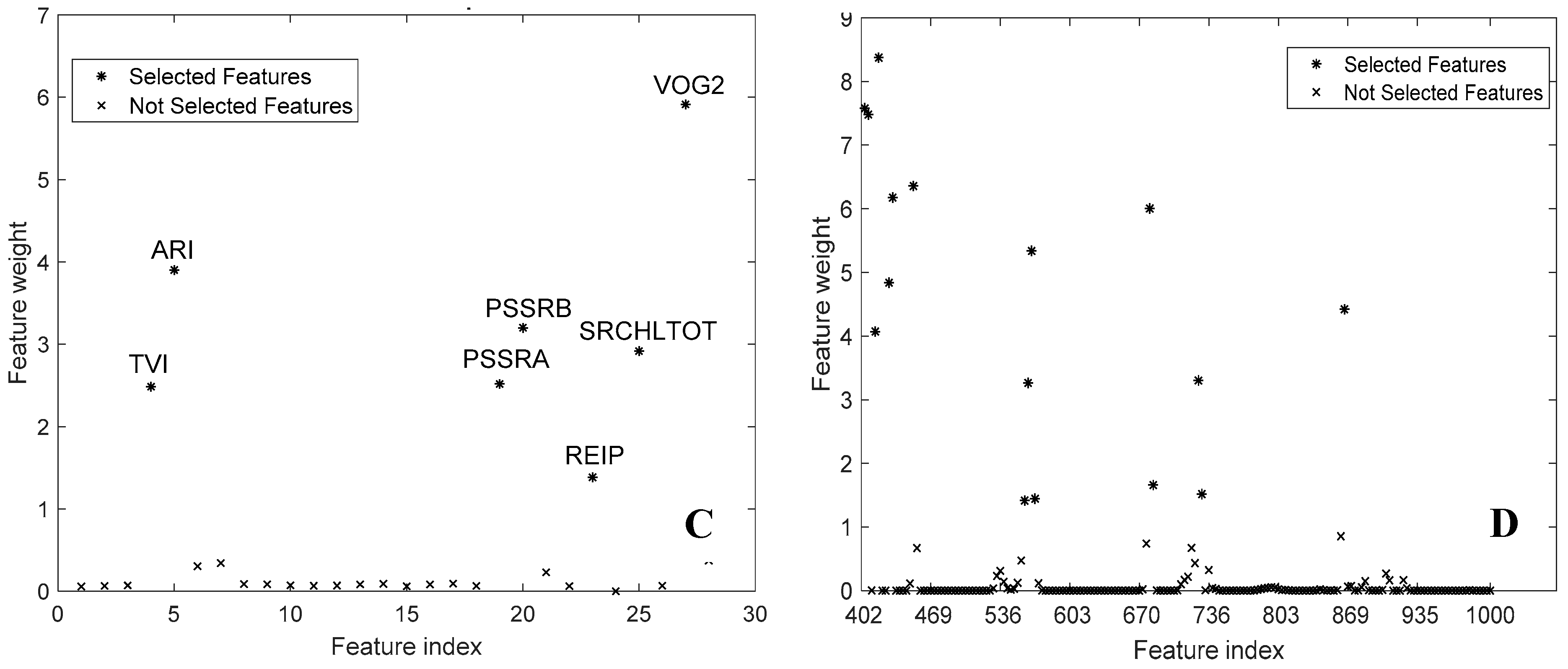
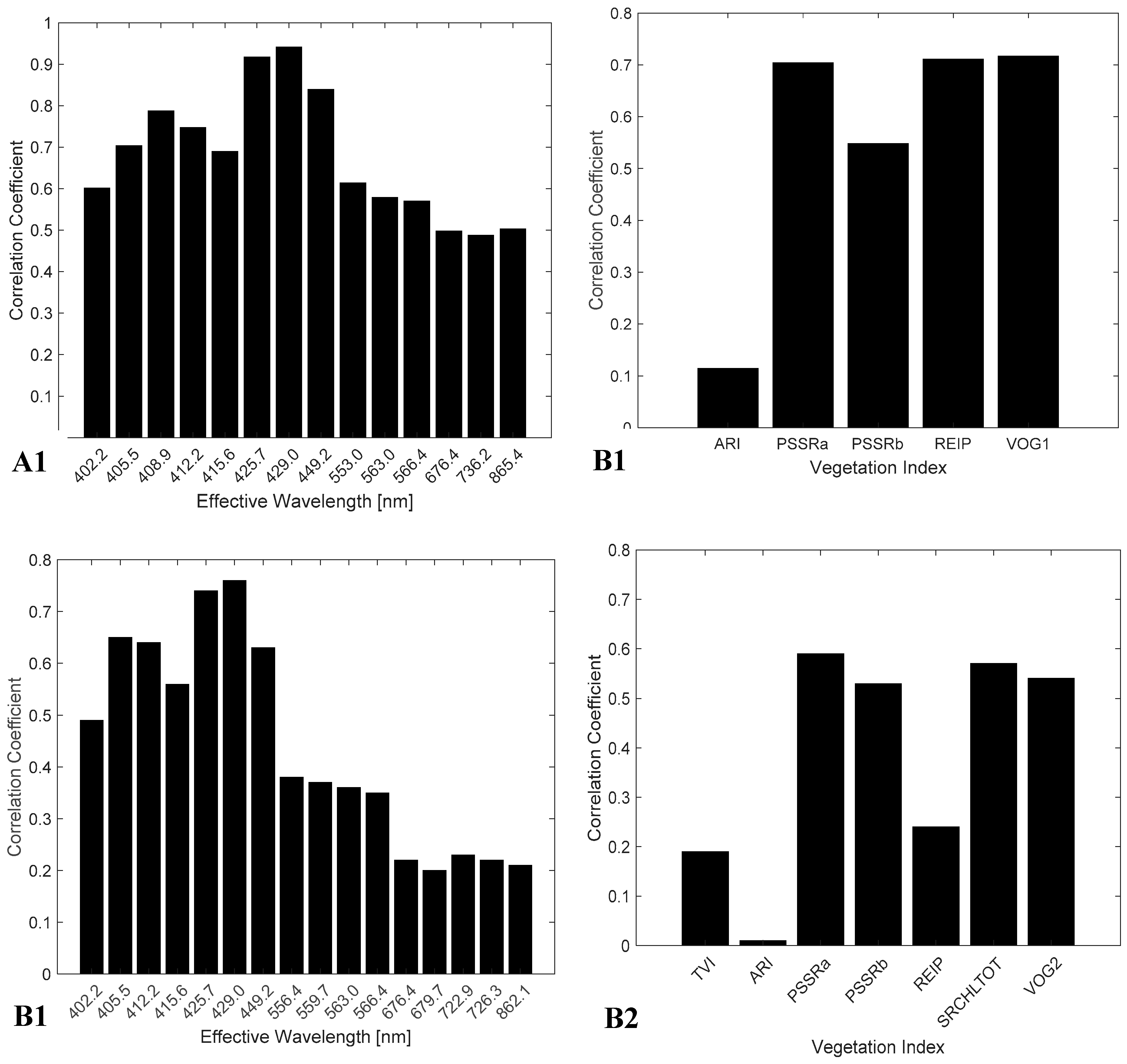
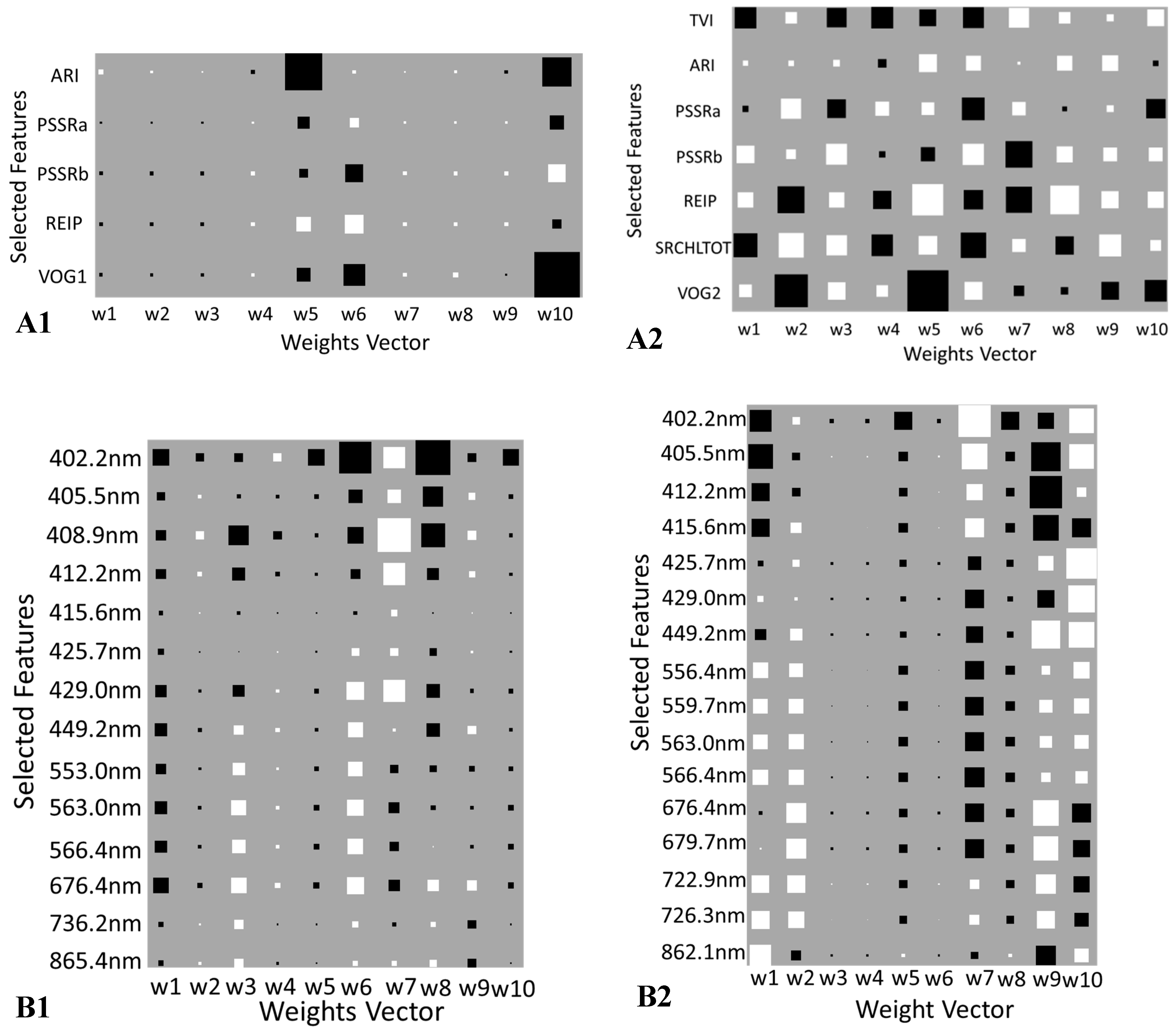
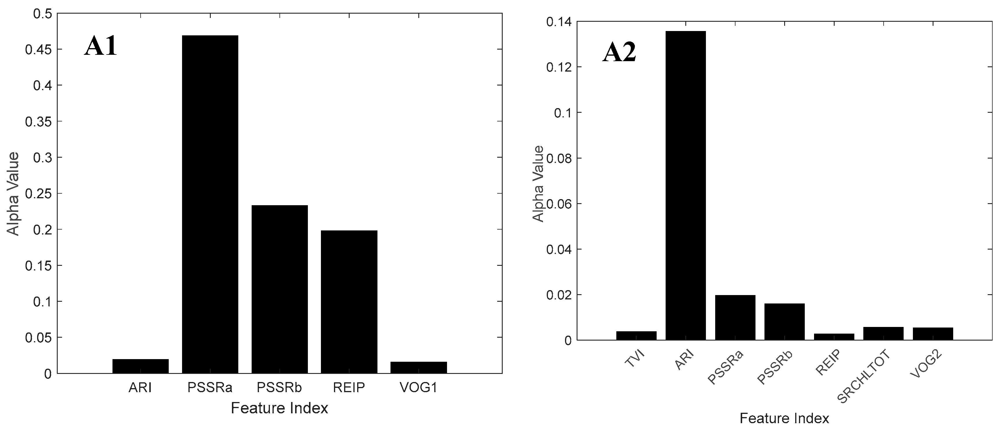
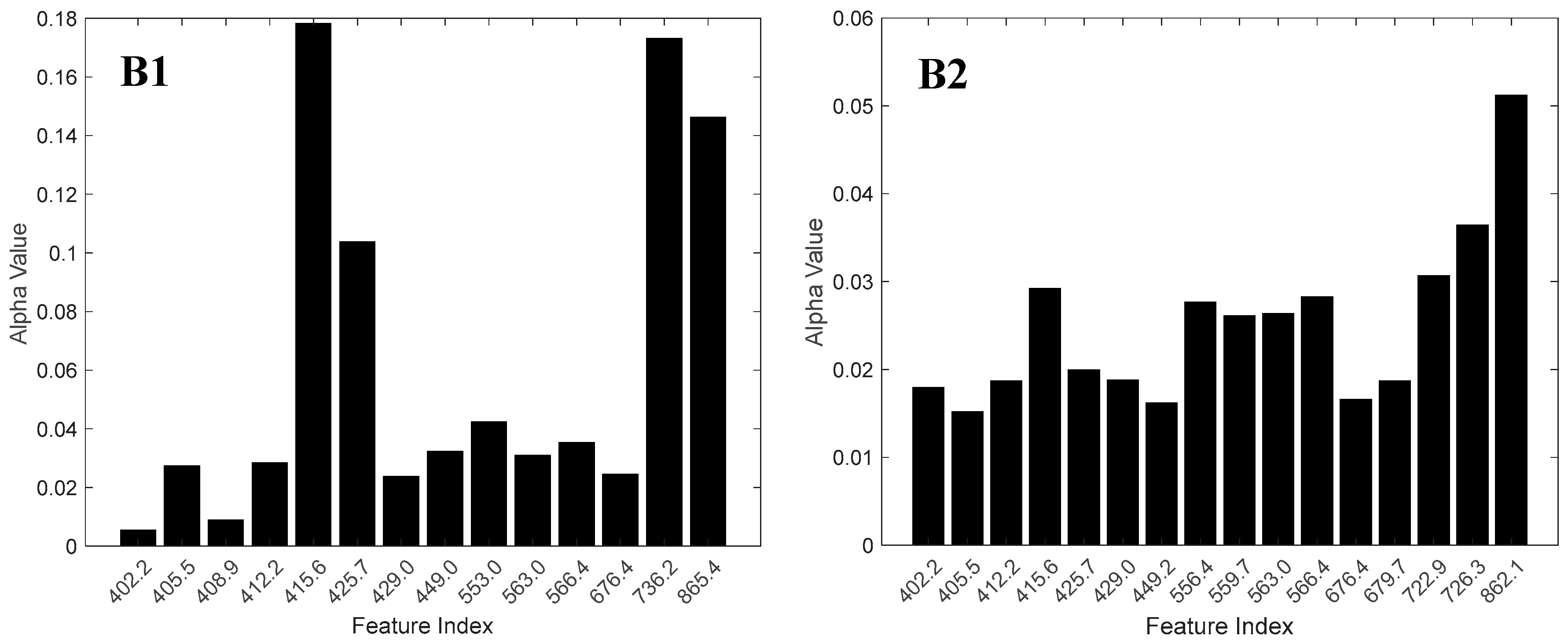
3.2. Feature Selection

As was mentioned, NCA was used for the feature selection of both VIs and EWs, and any spectral index or spectral value that had a feature weight higher than 1.18, as was decided by NCA algorithm, was included as an input feature in the classification process. The selected features for both the VIs and the effective wavelengths are shown in Figure 3.

The features that were selected by the NCA algorithm and that were used as input for the classification algorithms are also shown in

Table 4. Vegetation indices and effective wavelengths that were selected by the NCA algorithm as the input features for the selected classifiers before and after the outlier elimination.

Before Outlier Elimination		After Outlier Elimination
Vegetation Indices	Effective Wavelenghts (nm)	Vegetation Indices	Effective Wavelenghts (nm)
ARI PSSRa PSSRb REIP VOG1	402.2 405.5 408.9 412.2 415.6 425.7 429.0 449.2 553.0 563.0 566.4 676.4 736.2 865.4	TVI ARI PSSRa PSSRb REIP SRCHLTOT VOG2	402.2 405.5 412.2 415.6 425.7 429.0 449.2 556.4 559.7 563.0 566.4 676.4 679.7 722.9 726.3 862.1

.

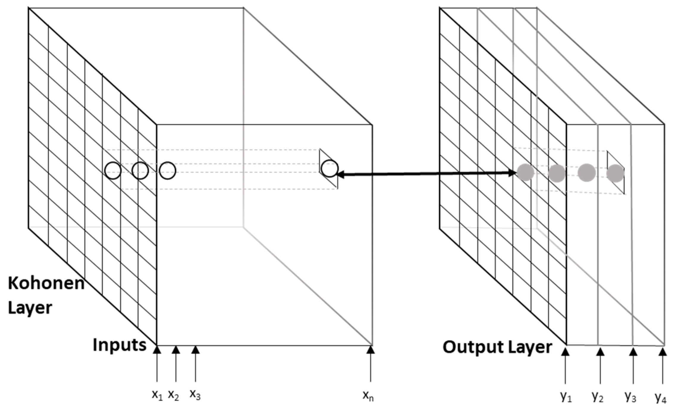
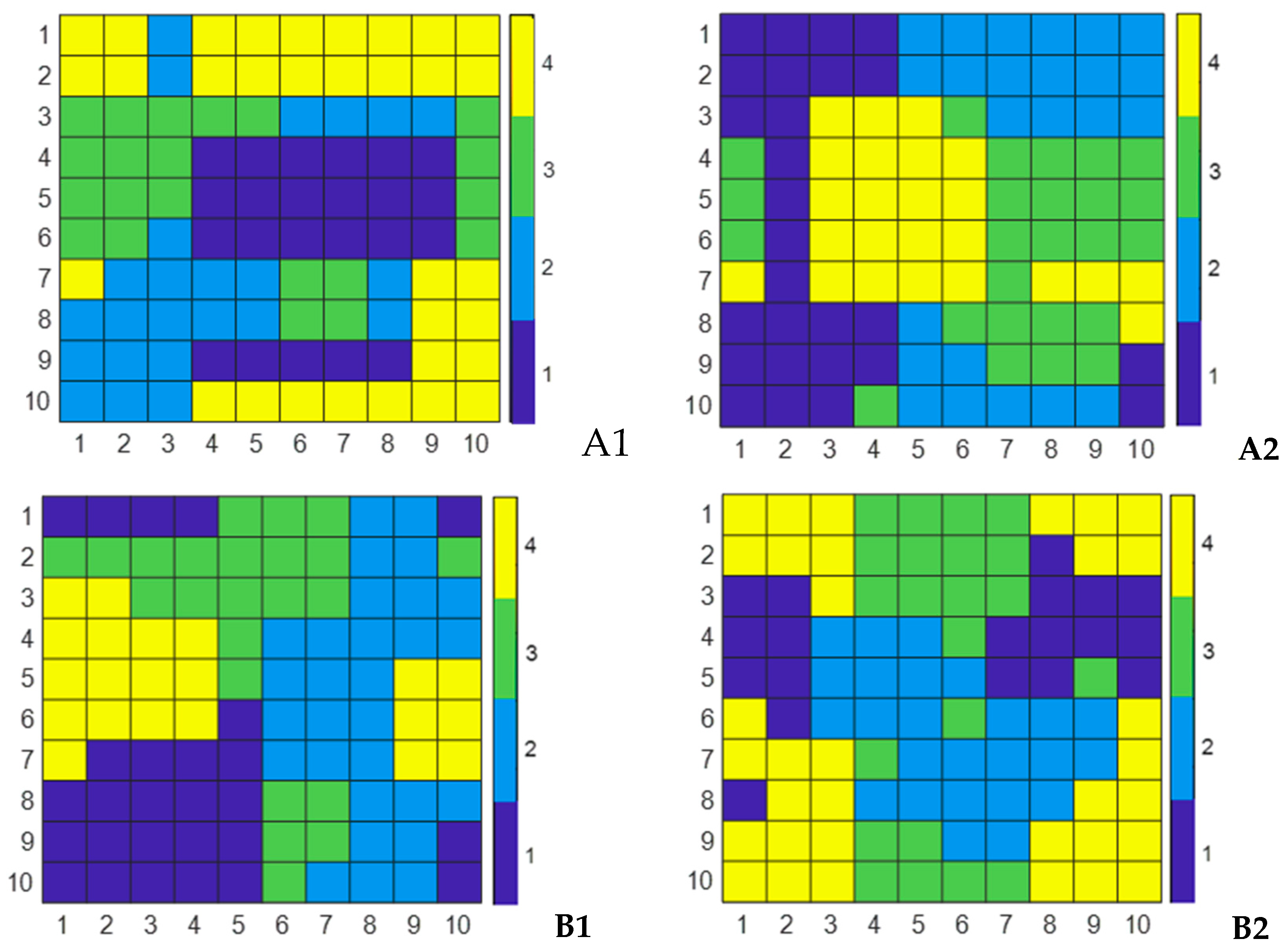
3.3. XY-F classifier

The performance of the XY-F classifier for the ToCV disease detection and its severity evaluation on the young tomato plants for the two different features set selected, before and after the outlier elimination, using the HR-PCA algorithm, are presented in

Table 5. XY – Fusion Network (XY-F) classifier prediction performance on the detection of Tomato Chlorosis Virus (ToCV) on the tomato plants and its severity before outlier elimination. Class 1 represents the healthy state and classes 2–4 the severity of the disease in an increasing order, denoted as ToCV1–ToCV3.

Outliers	Features	Class Prediction Accuracy (%)				Overall	F1 Score
		Healthy	ToCV1	ToCV2	ToCV3
Before Elimination	Effective Wavelengths (EW)	87.6	82.6	86.2	88.0	86.1	0.861
	Vegetation Indices (VI)	92.9	91.7	89.0	88.2	90.4	0.904
After Elimination	Effective Wavelengths (EW)	99.8	99.8	100	100	99.8	0.998
	Vegetation Indices (VI)	99.9	99.9	100	100	99.9	0.999

. Out of the 2984 total spectral signatures that were collected during the experimental process, from the 156 plants, 2089 were used for the training phase of the classifiers and 895 for their validation.

A closer look to Table 5 shows that EWs showed a slightly lower prediction accuracy in comparison with the VIs’ prediction accuracy for both outlier regimes (before and after outlier elimination); when the effective wavelengths (EW) were used as features, the prediction accuracy was always slighter lower in comparison with the respective outcome that the vegetation indices (VI) showed when they were selected as features This difference varied from 0%, in the case of class 3 and 4 (ToCV2 and ToCV3) prediction for the model that used the data after the outlier elimination, to 5.7% in the case of class 1 prediction for the model that used the data before the outlier elimination. It seems that the overall accuracy and F1 scores do not have any significant differences to each other. The best performing combination of classifier and feature selection was found to be the MLP–ARD classifier with vegetation indices as features.

The elimination of the outliers seemed to have a very significant influence in the models’ predictive accuracy, as the results were very close or even equal to the perfect 100% score for classes 3 and 4. The variance in the accuracy results before the outlier elimination was 4.53 for the EW features and 3.68 for the VI features, while after the outliers’ elimination, the variance was less than 0.05 for both feature sets.

The XY-F component maps for both of the feature sets that were selected for the models before and after the outlier elimination are presented in Figure 4. These component maps show the spatial distribution of the classes in the SOM plane, and they can better demonstrate that clusters from various pixels of the imagery can have similar characteristics while being spatially dispersed in the image [29]. The component maps seem to have a uniformity (measured to be more than 80% for each component map) in the class assignation for both the models before and after the outlier elimination. This means that the correlation coefficient of the input SOM layers and the class layers should show the influence of each feature in the model structure.

The correlation between the topological structure of the components map and the respective structure that was generated by the training vectors through their training phase is explained in Figure 5. It is apparent that for the model before the outlier elimination, 408.9, 425.7, 429.0 and 449.2 nm overruled the other EWs in terms of topological correlation to the component map when the EWs were used as features. Nevertheless, the rest of the EWs also played a significant role in the classifier as almost all of them had a correlation coefficient higher than 0.5. A similar pattern was followed for the model that was created after the outlier elimination. The difference is that although the maximum peaks were in the same exact places as in the respective model before the outlier elimination, after this point, the correlation fell to levels below 0.4.

On the other hand, when VIs were used as features, before the outlier elimination it was found that PSSRa, REIP and VOG1 showed a great correlation (r = 0.7) with PSSRb following and ARI playing a minor role contributing only a little to the model creation, having an r value close to 0.1 (Figure 5). Similarly, for the model that was created after the outlier elimination, the SRCHLTOT feature seemed to also have a large correlation alongside PSSRa, PSSRb and VOG2, while REIP and TVI had a minor correlation, and ARI once again had almost no correlation.

3.4. MLP–ARD Classifier

As far as the MLP–ARD classifier is concerned, its performance in detecting the ToCV disease and its severity level on the young tomato plants for the two different features set selected, before and after the outlier elimination, are presented in

Table 6. Multilayer Perceptron with Automated Relevance Detection (MLP-ARD) classifier prediction performance of the detection of ToCV on the tomato plants and its severity before outlier elimination. Class 1 represents the healthy state and classes 2–4 the severity of the disease in an increasing order, denoted as ToCV1–ToCV3.

Outliers	Features	Class Prediction Accuracy (%)				Overall	F1 Score
		Healthy	ToCV1	ToCV2	ToCV3
Before Elimination	EW	91.4	92.8	91.2	90.7	91.6	0.915
	VI	94.7	92.9	92.4	90.7	92.7	0.927
After Elimination	EW	100	100	100	100	100	1
	VI	100	100	100	100	100	1

Once again, out of the 2984 total spectral signatures that were collected, 2089 were used for the training phase of the classifiers and 8895 for their validation.

Table 6 shows that the MLP–ARD algorithm seemed to have great classification performance, as all of the predicted accuracy values exceeded 90%. The model that used the VIs as features showed a slightly better performance, in comparison with the respective model that used the EWs as features, of all cases of the models that were created before the outlier elimination, except the case of class 4 (ToCV3), where the accuracy was the same in both cases. The maximum difference was 2.7% in the case of the prediction of class 1 (healthy leaves).

As shown in the same table, after the outlier elimination, the model showed a perfect 100% accuracy in classifying the leaves’ spectral signatures into the healthy or one of the ToCV severity level classes. The variance in the accuracy results before the outlier elimination was 0.61 for the EW features and 2.03 for the VI features, while after the outlier elimination, there was no variance for both feature sets.

The Hinton diagrams in Figure 6 depict the weight values connecting the input features in any of the cases that were tested in this study (before and after outlier elimination and with EWs and VIs as input features) and is a better way of visualizing the function of the MLP–ARD algorithm [30]. The ARD algorithm suppresses the weights of the least important features and enforces the weights of the most active ones.

As seen in Figure 6, it is apparent that the biggest absolute weight values in case of the VIs used as input features were for ARI and VOG1 for the model before the outlier elimination. Additionally, it appears that in this very model the hidden neurons 1, 2, 3, 4, 7, 8 and 9 had a very small influence on the model’s performance. REIP, SR_CHLTOT and VOG2 were the respective indices that had the biggest absolute values, while ARI seemed to have almost no contribution to the model after outlier elimination. As far as the EWs input features are concerned, the range 402 to 412.2 nm seemed to have the highest impact in the model created before the outlier elimination, while the 415.6, 425.7, 736.2 and 865.4 nm seemed to have the lowest impact. On the other hand, in the Hinton diagram for the model that used the EWs input features after the outlier elimination, there was a uniformity in the impact that each EW had to the model. Only 862.1 nm seemed to have slightly smaller weight values.

As the training procedure went towards the last iterations, the highest L2 norms in the network were connected to the lowest alpha values and thus the highest weigh variances. Figure 7 shows the alpha hyperparameter values for the interconnection weights between the input and the hidden layer of the MLP. As seen in Figure 7, it was apparent that there was an inversely direct connection between the magnitude of the alpha hyperparameter and the weight values that were presented in the Hinton diagrams of Figure 6. Indeed, it appeared that ARI and VOG1 and TVI, REIP, SRCHLTOT and VOG2 had the lowest alpha values for the models before and after the outlier elimination, respectively. Although ARI had the highest alpha value in comparison with the rest of the features in the model that were created after the outlier elimination, this value was not as high when it was compared with the respective highest values of the model before the outlier elimination. Similarly, the EWs that appeared to have the highest alpha values were 415.6, 425.7, 736.2 and 865.4 nm for the model before the outlier elimination and 862.1 nm for the model after the outlier elimination. In the latter case it could be also observed that the maximum alpha value was close to 0.05, which was a relatively small value when compared with the respective data from Figure 7(B1).

4. Discussion

4.1. General and Spectral Data Overview

Spectral reflectance signature samples collected by the young tomato leaf surfaces were used in this study in order to detect a possible viral infection in an early stage, before the symptoms become visible on the leaf surface, and the infection severity. The selected virus was ToCV, because it is an emergent plant pathogen in tomato fields in Greece and worldwide [8,66]. The classifiers that were used were the XY-F network and the MLP–ARD.

From the comparison of the mean spectral responses of the healthy vs. infected plants in Figure 3, it was found that an increase of severity has as a consequence a decrease of the spectral response in the NIR region and a slight increase of the spectral response in the visible region (400–700 nm). This very slight increase in the spectral peak in the visible region (with the local maximum close to 550 nm) is clearly not detectable by human eyes as a visible symptom and is probably happening because as the ToCV infection becomes more serious, it affects the leaf pigments, causing interveinal chlorosis. Yellowing has appeared in a similar situation of sugarcane viral infection [57] to have a slightly increased reflectance percentage in the visible region of the spectrum. There was no shifting of the red edge region though to lower wavelengths, as happens when yellowing occurs to a leaf surface, according to Sims and Gamon [67].

A similar decrease in the red edge and NIR regions was shown by Grisham et al. [23] and Gazala et al. [68] that used hyperspectral imagery and spectral signatures by spectroradiometer to identify sugarcane viruses causing leaf yellowing. Additionally, healthy leaves have been found to show higher reflectance in the NIR region compared to those infected by tobacco mosaic virus (TMV), but the visible part seems to have the highest reflectance in the case of severe infection [26]. The NIR region reflectance pattern is caused by the internal light scattering by the leaf cells [46,68,69]. The change in the NIR reflectance in such a way could be explained by the effects of the virus infection [70] that induce the destruction of the cellular structures, which in turn cause the collapse of cell compactness and loss of air spaces.

4.2. The Effect of Outliers in the Models

It is apparent that outlier elimination gave a more discernible profile in the average spectral signatures in the NIR region by segregating the four different classes in terms of infection severity in descending reflectance order, despite the loss of visible symptoms (Figure 3). This process showed a significant improvement of the performance of the classifiers used in this study, in most of the cases, to score a perfect accuracy and F1 score. This was also confirmed by the literature on the effect of outlier elimination in the classification process [70]. The reason for this remarkable improvement in these models is probably due to the spectral instrument (spectrometer) used having a clip that totally isolates the leaf from the external disturbances. Additionally, the halogen light source of the instrument is fixed on the clip and almost in direct contact with the leaf surface, and thus it does not allow heat fluctuations.

Nevertheless, it should be noted that most of the error occurring during classification to the models before outlier elimination was probably due to spectral signature overlap of different classes. Indeed, unpublished data from the confusion matrices that were created showed that most of the misclassification errors in the models were between consecutive classes, i.e., class 1 and 2 and class 3 and 4, and there were hardly any errors occurring between classes 1 and 3, 2 and 4, and 1 and 4 and very few between classes 2 and 3, meaning that some signatures from healthy leaves were classified as slightly infected and vice versa and some signatures from mid infected leaves were misclassified as severely infected.

Spectral signatures are very close to each other before outlier elimination (Figure 3) making it probable that signatures belonging to the limits of neighboring classes (Table 3) were classified wrongly due to overlap of signatures. Absence of outliers in this case could raise some robustness issues in case of a similar experiment. Thus, it is possible that the collected data containing the outliers may perform a better generalization of the proposed models for either online application or virus detection, and its severity in similar cases, in comparison to the models after the outlier elimination.

4.3. Spectral Bands and Vegetation Indices Selected by NCA

Figure 8 shows the spectral bands that were selected by the NCA algorithm and that were used for the classification either as EWs or as a structural part of the VI formula. This figure shows that the selected bands cover parts from most of the important regions (peak in the visible part, red edge and the peak and parts from the NIR plateau region) of the spectrum for both models before and after the outlier elimination, for the detection of the vegetation health, as was described by Kalacska and Sanchez-Azofeifa [71]. The difference between VIs and EWs is that there are also bands in the EWs that cover the range from 400 to 450 nm, which does not happen in the case of the VIs. In this paper it was found that the bands in that region can have a significant role in the model predictive accuracy, having in most cases high correlation coefficient in the case of the XY-F network (Figure 5) and low alpha values in the case of MLP–ARD classifier (Figure 7), which is also in accordance with the findings of Zhu et al. [26], which had 459.58 nm selected as the most influential spectral band feature, using the successive projections algorithm (SPA).

It is known that the reflectance peak in the visible part of the spectrum is related to and dependent on the chlorophyll a and b, carotenoid and anthocyanin concentrations. The selection of bands in the region of 400 to 450 nm could be probably related to the chlorophyll concentration, while the peak around 550 nm could be related to anthocyanin absorption

The VIs that were chosen in this paper by the NCA algorithm combine spectral bands from both the visible part of the spectrum and the part close to or on the red edge, taking into account that these two regions makes it easier for the algorithm to differentiate any changes that happen either in the shifting of the local minima to higher or lower values or to the shifting of the red edge inflection point to the left or the right. This is probably why the REIP index was chosen for both outlier existence scenarios. REIP was also found to be useful for the detection of vegetation health by Hoque and Hutzler [72] and Vogelmann et al. [56]. Nevertheless, owing to the fact that there was almost no change of the position of the inflection point to higher or lower wavelengths, this index was found to have in most of the cases an average contribution to the model’s performance (Figure 5(B2) and Figure 7(A1)).

Simple ratio indices, like PSSRa and PSSRb, for the direct chlorophyll content estimation were also selected for both model scenarios. For the models created after the outlier elimination there was also the SR_CHLTOT index selected (Table 2). Indeed, chlorophyll is the most important pigment for the photosynthesis and is thus one of the most important indicators for the general health condition of the plant [73]; this is why these indices had such an important contribution to the models, as can be seen in Figure 5 and Figure 7. These findings are in accordance with the respective findings of Lu et al. [74], who investigated the contribution of different VIs to the detection of tomato leaf health condition and found a high contribution of the PSSR index.

VOG1 and VOG2 are both spectral indices that deal with the changes that occur in the red edge zone, and according to Figure 5 and Figure 7, they are proven to have a major effect on the models’ efficiency. This is comparable with the related works of Lu et al. [74] and Lopez et al. [75], that have found a dominant effect of VOG index for disease detection (including viral infection) in an early stage in almond trees and tomato plants, respectively.

Finally, ARI is a VI that is generally used for the estimation of the anthocyanins and is also a VI that was selected for both outlier scenarios in this study. Despite this fact though and the fact that ToCV infection induces increased anthocyanin accumulation in some tomato cultivars [76], the results from the classifiers showed a very low importance of this index for both XY-F network and one case of the MLP–ARD models (Figure 5 and Figure 7). There is a conflict in these findings in comparison with those of Devadas et al. [77], who found that ARI is a very efficient indicator for the differentiation of three different rust types. It is probable that either the contribution of ARI in the present paper’s models’ efficiency was overruled by the contribution of the rest of the VIs that were selected by NCA algorithm, or there was no effect on the anthocyanin content caused by ToCV in this tomato cultivar.

4.4. Classifier Results

An overview of the results for both models created before and after the outlier elimination reveals the great performance that was achieved in all the cases that were studied, scoring individual class accuracies higher than 80% in the case of the XY-F network (Table 5) and higher than 90% in the case of the MLP–ARD ANN (Table 6). The performance of the models, before the outlier elimination, described in this paper are comparable with the findings of Schor et al. [78] for the detection of tomato spotted wilt virus, using PCA, with an overall accuracy of 90%, and Xu et al. [39] for the detection of tobacco mosaic virus using a Mahalanobis distance based model.

Despite the fact that in this paper MLP–ARD generally showed better performance than the XY-F network, previous studies [29,30] that have worked on a dataset for the detection of a fungal infection on S. Marianum weed plants have shown that hierarchical self-organizing models like the XY-F network showed a better overall performance in comparison to the MLP–ARD algorithm. Using the EWs as input features, a slightly lower overall performance was found than with VIs and a higher variance between the models before and after the outlier elimination.

A comparison between the two different aspects of the classifiers that were employed in this paper showed that if we excluded the models that were created after the outlier elimination and had a perfect performance, the best performing combination of classifier and feature selection was found to be the MLP–ARD classifier with VIs as features. This is probably due to the fact that the VIs were developed in such a way as to reveal the structural and metabolic alterations that happen in plant leaves when they are subjected to a stress regime, by fusing the combined effect of two or more spectral bands from the most important regions of the spectrum in one formula.

A close observation of the results of the Hinton diagram in Figure 6 shows that most of the hidden neurons in the best performing VIs (REIP, SR_CHLTOT and VOG2) in the case of the model after the outlier elimination have opposite signs (positive and negative weight values). This could be an indicator that there is very low overlap between the features, and at the same time a synergistic activity, which in turn is an indicator of feature fusion by the classifier performed by the ARD algorithm.

Finally, there was a balanced distribution of the selected signatures for each class from the comparison of the very low absolute difference between the F1 score and accuracy values, for every model. This means that accuracy, an evaluation metric prone to imbalanced data, can be used in this study to give a satisfactory estimation of the detector’s performance.

5. Conclusions

In the present study, the spectral reflectance signatures of ToCV-infected tomato plants were studied for the detection of a possible virus infection and a quantitative severity level estimation by applying machine learning techniques on selected spectral features of these plants. A non-destructive disease detection approach is of value for the early prevention of the disease spread in a nursery or farm level and the subsequent loss of production.

Both XY-F network and MLP–ARD ANN classifiers were demonstrated to be greatly efficient in detecting the ToCV infection and its severity level, scoring an overall accuracy of over 85%. MLP–ARD seems to perform generally better than the XY-F classifier and also shows more robust results in terms of variance.

Outlier elimination plays a major role in the overall performance of the classifiers, showing a perfect accuracy when they are eliminated for both classifiers. Outlier existence though, could be a valuable tool for the generalization of the model for reasons of repetition of the experiment in similar situations, as they take into account the possible class overlap that happens between the spectral signatures of neighbor classes, given that there is no other possible reason for outlier existence, due to the high resolution of the spectrometer measurements.

VIs were shown to have a slightly better overall performance in comparison to the effective wavelengths that were chosen by the NCA algorithm. A combination of pigment specific indices like PSSRa, PSSRb, SR_CHLTOT and ARI and red edge alteration vegetation indices like VOG1, VOG2 and REIP are found to be the most appropriate for the classification process and its performance.

References

1. Liakos, K.G.; Busato, P.; Moshou, D.; Pearson, S.; Bochtis, D. Machine learning in agriculture: A review. Sensors 2018, 18, 2674. [Google Scholar] [CrossRef] [PubMed] [Green Version]
2. Mulla, D.J. Twenty five years of remote sensing in precision agriculture: Key advances and remaining knowledge gaps. Biosyst. Eng. 2013, 114, 358–371. [Google Scholar] [CrossRef]
3. Golhani, K.; Balasundram, S.K.; Vadamalai, G.; Pradhan, B. A review of neural networks in plant disease detection using hyperspectral data. Inf. Process. Agric. 2018, 5, 354–371. [Google Scholar] [CrossRef]
4. Berdugo, C.A.; Mahlein, A.K.; Steiner, U.; Dehne, H.W.; Oerke, E.C. Sensors and imaging techniques for the assessment of the delay of wheat senescence induced by fungicides. Funct. Plant Biol. 2013, 40, 677–689. [Google Scholar] [CrossRef] [PubMed]
5. Mahlein, A.K.; Kuska, M.T.; Behmann, J.; Polder, G.; Walter, A. Hyperspectral sensors and imaging technologies in phytopathology: State of the art. Annu. Rev. Phytopathol. 2018, 56, 535–558. [Google Scholar] [CrossRef]
6. Mahlein, A.K.; Oerke, E.C.; Steiner, U.; Dehne, H.W. Recent advances in sensing plant diseases for precision crop protection. Eur. J. Plant Pathol. 2012, 133, 197–209. [Google Scholar] [CrossRef]
7. Wintermantel, W.M.; Wisler, G.C. Vector specificity, host range, and genetic diversity of Tomato chlorosis virus. Plant Dis. 2006, 90, 814–819. [Google Scholar] [CrossRef] [Green Version]
8. Orfanidou, C.G.; Dimitriou, C.; Papayiannis, L.C.; Maliogka, V.I.; Katis, N.I. Epidemiology and genetic diversity of criniviruses associated with tomato yellows disease in Greece. Virus Res. 2014, 186, 120–129. [Google Scholar] [CrossRef]
9. Fiallo-Olive, E.; Navas-Castillo, J. Tomato chlorosis virus, an emergent plant virus still expanding its geographical and host ranges. Mol. Plant Pathol. 2019, 20, 1307–1320. [Google Scholar] [CrossRef] [Green Version]
10. Wisler, G.C.; Li, R.-H.; Liu, H.Y.; Lowry, D.S.; Duffus, J.E. Tomato Chlorosis Virus: A New Whitefly-Transmitted, Phloem-Limited, Bipartite Closterovirus of Tomato. Phytopathology 1998, 88, 402–409. [Google Scholar] [CrossRef] [Green Version]
11. Gold, K.M.; Townsend, P.A.; Chlus, A.; Herrmann, I.; Couture, J.J.; Larson, E.R.; Gevens, A.J. Hyperspectral Measurements Enable Pre-Symptomatic Detection and Differentiation of Contrasting Physiological Effects of Late Blight and Early Blight in Potato. Remote Sens. 2020, 12, 286. [Google Scholar] [CrossRef] [Green Version]
12. Fernández, C.I.; Leblon, B.; Haddadi, A.; Wang, K.; Wang, J. Potato late blight detection at the leaf and canopy levels based in the red and red-edge spectral regions. Remote Sens. 2020, 12, 1292. [Google Scholar] [CrossRef] [Green Version]
13. Herrmann, I.; Berenstein, M.; Paz-Kagan, T.; Sade, A.; Karnieli, A. Spectral assessment of two-spotted spider mite damage levels in the leaves of greenhouse-grown pepper and bean. Biosyst. Eng. 2017, 157, 72–85. [Google Scholar] [CrossRef]
14. Papayiannis, L.C.; Harkou, I.S.; Markou, Y.M.; Demetriou, C.N.; Katis, N.I. Rapid discrimination of Tomato chlorosis virus, Tomato infectious chlorosis virus and co-amplification of plant internal control using real-time RT-PCR. J. Virol. Methods 2011, 176, 53–59. [Google Scholar] [CrossRef]
15. Duffus, J.E.; Liu, H.Y.; Wisler, G.C. Tomato infectious chlorosis virus—A new clostero-like virus transmitted by Trialeurodes vaporariorum. Eur. J. Plant. Pathol. 1996, 102, 219–226. [Google Scholar] [CrossRef]
16. Jacquemond, M.; Verdin, E.; Dalmon, A.; Guilbaud, L.; Gognalons, P. Serological and molecular detection of Tomato chlorosis virus and Tomato infectious chlorosis virus in tomato. Plant. Pathol. 2009, 58, 210–220. [Google Scholar] [CrossRef]
17. Morris, J.; Steel, E.; Smith, P.; Boonham, N.; Spence, N.; Barker, I. Host range studies for Tomato chlorosis virus and Cucumber vein yellowing virus transmitted by Bemisia tabaci (Gennadius). Eur. J. Plant. Pathol. 2005, 114, 265–273. [Google Scholar] [CrossRef]
18. Thomas, S.; Kuska, M.T.; Bohnenkamp, D.; Brugger, A.; Alisaac, E.; Wahabzada, M.; Behman, J.; Mahlein, A.K. Benefits of hyperspectral imaging for plant disease detection and plant protection: A technical perspective. J. Plant Dis. Prot. 2018, 125, 5–20. [Google Scholar] [CrossRef]
19. Guan, J.; Nutter, F.W., Jr. Relationships between defoliation, leaf area index, canopy reflectance, and forage yield in the alfalfa-leaf spot pathosystem. Comput. Electr. Agric. 2002, 37, 97–112. [Google Scholar] [CrossRef]
20. West, J.S.; Bravo, C.; Oberti, R.; Lemaire, D.; Moshou, D.; McCartney, H.A. The potential of optical canopy measurements for targeted control of field crop diseases. Ann. Rev. Phytopathol. 2003, 41, 593–614. [Google Scholar] [CrossRef] [Green Version]
21. Bravo, C.; Moshou, D.; West, J.; McCartney, A.; Ramon, H. Early disease detection in wheat fields using spectral reflectance. Biosyst. Eng. 2003, 84, 137–145. [Google Scholar] [CrossRef]
22. Moshou, D.; Bravo, C.; Oberti, R.; West, J.; Bodria, L.; McCartney, A.; Ramon, H. Plant disease detection based on data fusion of hyper-spectral and multi-spectral fluorescence imaging using Kohonen maps. Real Time Imaging 2005, 11, 75–83. [Google Scholar] [CrossRef]
23. Grisham, M.P.; Johnson, R.M.; Zimba, P.V. Detecting Sugarcane yellow leaf virus infection in asymptomatic leaves with hyperspectral remote sensing and associated leaf pigment changes. J. Virol. Methods 2010, 167, 140–145. [Google Scholar] [CrossRef] [PubMed]
24. Bürling, K.; Hunsche, M.; Noga, G. Presymptomatic Detection of Powdery Mildew Infection in Winter Wheat Cultivars by Laser-Induced Fluorescence. Appl. Spectrosc. 2012, 66, 1411–1419. [Google Scholar] [CrossRef] [PubMed]
25. Arens, N.; Backhaus, A.; Döll, S.; Fischer, S.; Seiffert, U.; Mock, H.-P. Non-invasive Presymptomatic Detection of Cercospora beticola Infection and Identification of Early Metabolic Responses in Sugar Beet. Front. Plant Sci. 2016, 7, 1377. [Google Scholar] [CrossRef] [Green Version]
26. Zhu, H.; Chu, B.; Zhang, C.; Liu, F.; Jiang, L.; He, Y. Hyperspectral imaging for presymptomatic detection of tobacco disease with successive projections algorithm and machine-learning classifiers. Sci. Rep. 2017, 7, 4125. [Google Scholar] [CrossRef] [Green Version]
27. Moshou, D.; Bravo, C.; West, J.; Wahlen, S.; McCartney, A.; Ramon, H. Automatic detection of ‘yellow rust’ in wheat using reflectance measurements and neural networks. Comput. Electron. Agric. 2004, 44, 173–188. [Google Scholar] [CrossRef]
28. Moshou, D.; Bravo, C.; Oberti, R.; West, J.S.; Ramon, H.; Vougioukas, S.; Bochtis, D. Intelligent multi-sensor system for the detection and treatment of fungal diseases in arable crops. Biosyst. Eng. 2011, 108, 311–321. [Google Scholar] [CrossRef]
29. Pantazi, X.E.; Tamouridou, A.A.; Alexandridis, T.K.; Lagopodi, A.L.; Kashefi, J.; Moshou, D. Evaluation of hierarchical self-organising maps for weed mapping using UAS multispectral imagery. Comput. Electron. Agric. 2017, 139, 224–230. [Google Scholar] [CrossRef]
30. Tamouridou, A.; Pantazi, X.; Alexandridis, T.; Lagopodi, A.; Kontouris, G.; Moshou, D. Spectral identification of disease in weeds using multilayer perceptron with automatic relevance determination. Sensors 2018, 18, 2770. [Google Scholar] [CrossRef] [Green Version]
31. Mishra, P.; Asaari, M.S.M.; Herrero-Langreo, A.; Lohumi, S.; Diezma, B.; Scheunders, P. Close range hyperspectral imaging of plants: A review. Biosyst. Eng. 2017, 164, 49–67. [Google Scholar] [CrossRef]
32. Bannari, A.; Morin, D.; Bonn, F.; Huete, A.R. A review of vegetation indices. Remote Sens. Rev. 1995, 13, 95–120. [Google Scholar] [CrossRef]
33. Haas, J.; Lozano, E.R.; Poppy, G.M. A simple, light clip-cage for experiments with aphids. Agric. For. Entomol. 2018, 20, 589–592. [Google Scholar] [CrossRef]
34. Orfanidou, C.G.; Pappi, P.G.; Efthimiou, K.E.; Katis, N.I.; Maliogka, V.I. Transmission of Tomato chlorosis virus (ToCV) by Bemisiatabaci biotype Q and evaluation of four weed species as viral sourced. Plant Dis. 2016, 100, 2043–2049. [Google Scholar] [CrossRef] [PubMed] [Green Version]
35. Morellos, A.; Pantazi, X.E.; Moshou, D.; Alexandridis, T.; Whetton, R.; Tziotzios, G.; Wiebensohn, J.; Bill, R.; Mouazen, A.M. Machine learning based prediction of soil total nitrogen, organic carbon and moisture content by using VIS-NIR spectroscopy. Biosyst. Eng. 2016, 152, 104–116. [Google Scholar] [CrossRef] [Green Version]
36. Kochubey, S.M.; Kazantsev, T.A. Derivative vegetation indices as a new approach in remote sensing of vegetation. Front. Earth Sci. 2012, 6, 188–195. [Google Scholar] [CrossRef]
37. Yao, X.; Ren, H.; Cao, Z.; Tian, Y.; Cao, W.; Zhu, Y.; Cheng, T. Detecting leaf nitrogen content in wheat with canopy hyperspectrum under different soil backgrounds. Int. J. Appl. Earth Obs. Geoinf. 2014, 32, 114–124. [Google Scholar] [CrossRef]
38. Savitzky, A.; Golay, M.J. Smoothing and differentiation of data by simplified least squares procedures. Anal. Chem. 1964, 36, 1627–1639. [Google Scholar] [CrossRef]
39. Xu, H.; Caramanis, C.; Mannor, S. Outlier-robust PCA: The high-dimensional case. IEEE Trans. Inf. Theory 2013, 59, 546–572. [Google Scholar] [CrossRef] [Green Version]
40. Mahlein, A.K.; Rumpf, T.; Welke, P.; Dehne, H.W.; Plümer, L.; Steiner, U.; Oerke, E.C. Development of spectral indices for detecting and identifying plant diseases. Remote Sens. Environ. 2013, 128, 21–30. [Google Scholar] [CrossRef]
41. Rouse, J.W.; Hass, R.H.; Schell, J.A.; Deering, D.W. Monitoring Vegetation Systems in the Great Plains with ERTS. In Proceedings of the Third Earth Resources Technology Satellite-1 Symposium, Washington, DC, USA, 10–14 December 1972. [Google Scholar]
42. Liu, L.; Huang, W.; Pu, R.; Wang, J. Detection of Internal Leaf Structure Deterioration Using a New Spectral Ratio Index in the Near-Infrared Shoulder Region. J. Integr. Agric. 2014, 13, 760–769. [Google Scholar] [CrossRef]
43. Barnes, E.M.; Clarke, T.R.; Richards, S.E.; Colaizzi, P.D.; Haberland, J.; Kostrzewski, M.; Lascano, R.J. Coincident detection of crop water stress, nitrogen status and canopy density using ground based multispectral data. In Proceedings of the Fifth International Conference on Precision Agriculture, Bloomington, MN, USA, 16–19 July 2000; Volume 1619. [Google Scholar]
44. Broge, N.H.; Leblanc, E. Comparing prediction power and stability of broadband and hyperspectral vegetation indices for estimation of green leaf area index and canopy chlorophyll density. Remote Sens. Environ. 2001, 76, 156–172. [Google Scholar] [CrossRef]
45. Gitelson, A.A.; Gritz, Y.; Merzlyak, M.N. Relationships between leaf chlorophyll content and spectral reflectance and algorithms for non-destructive chlorophyll assessment in higher plant leaves. J. Plant Physiol. 2003, 160, 271–282. [Google Scholar] [CrossRef] [PubMed]
46. Carter, G.A. Ratios of leaf reflectances in narrow wavebands as indicators of plant stress. Remote Sens. 1994, 15, 697–703. [Google Scholar] [CrossRef]
47. Gitelson, A.A.; Merzlyak, M.N. Remote estimation of chlorophyll content in higher plant leaves. Int. J. Remote Sens. 1997, 18, 2691–2697. [Google Scholar] [CrossRef]
48. Datt, B. Remote sensing of chlorophyll a, chlorophyll b, chlorophyll a + b, and total carotenoid content in eucalyptus leaves. Remote Sens. Environ. 1998, 66, 111–121. [Google Scholar] [CrossRef]
49. Datt, B. A new reflectance index for remote sensing of chlorophyll content in higher plants: Tests using Eucalyptus leaves. J. Physiol. 1999, 154, 30–36. [Google Scholar] [CrossRef]
50. Lichtenthaler, H.K.; Gitelson, A.; Lang, M. Non-Destructive Determination of Chlorophyll Content of Leaves of a Green and an Aurea Mutant of Tobacco by Reflectance Measurements. J. Plant Physiol. 1996, 148, 483–493. [Google Scholar] [CrossRef]
51. Haboudane, D.; Miller, J.R.; Pattey, E.; Zarco-Tejada, P.J.; Strachan, I.B. Hyperspectral vegetation indices and novel algorithms for predicting green LAI of crop canopies: Modeling and validation in the context of precision agriculture. Remote Sens. Environ. 2004, 90, 337–352. [Google Scholar] [CrossRef]
52. Blackburn, G.A. Quantifying chlorophylls and carotenoids at leaf and canopy scales: An evaluation of some hyperspectral approaches. Remote Sens. Environ. 1998, 66, 273–285. [Google Scholar] [CrossRef]
53. Roujean, J.-L.; Breon, F.-M. Estimating PAR absorbed by vegetation from bidirectional reflectance measurements. Remote Sens. Environ. 1995, 51, 375–384. [Google Scholar] [CrossRef]
54. Dawson, T.P.; Curran, P.J. Technical note A new technique for interpolating the reflectance red edge position. Int. J. Remote Sens. 1998, 19, 2133–2139. [Google Scholar] [CrossRef]
55. Guyot, G.; Baret, F.; Major, D.J. High spectral resolution: Determination of spectral shifts between the red and the near infrared. Int. Arch. Photogramm. Remote Sens. 1988, 11, 750–760. [Google Scholar]
56. Vogelmann, J.E.; Rock, B.N.; Moss, D.M. Red edge spectral measurements from sugar maple leaves. Remote Sens. 1993, 14, 1563–1575. [Google Scholar] [CrossRef]
57. Yang, W.; Wang, K.; Zuo, W. Neighborhood Component Feature Selection for High-Dimensional Data. J. Comput. 2012, 7, 161–168. [Google Scholar] [CrossRef]
58. Goldberger, J.; Hinton, G.E.; Roweis, S.T.; Salakhutdinov, R.R. Neighbourhood components analysis. In Advances in Neural Information Processing Systems; MIT Press: Cambridge, MA, USA, 2005; pp. 513–520. [Google Scholar]
59. Torresani, L.; Lee, K.C. Large margin component analysis. In Advances in Neural Information Processing Systems; MIT Press: Cambridge, MA, USA, 2007; pp. 1385–1392. [Google Scholar]
60. Raghu, S.; Sriraam, N. Classification of focal and non-focal EEG signals using neighborhood component analysis and machine learning algorithms. Expert Syst. Appl. 2018, 113, 18–32. [Google Scholar] [CrossRef]
61. Melssen, W.; Wehrens, R.; Buydens, L. Supervised Kohonen networks for classification problems. Chemom. Intell. Lab. Syst. 2006, 83, 99–113. [Google Scholar] [CrossRef]
62. Pantazi, X.E.; Moshou, D.; Oberti, R.; West, J.; Mouazen, A.M.; Bochtis, D. Detection of biotic and abiotic stresses in crops by using hierarchical self organizing classifiers. Precis. Agric. 2017, 18, 383–393. [Google Scholar] [CrossRef]
63. Bishop, C.M. Pattern Recognition and Machine Learning; Springer: Berlin, Germany, 1995. [Google Scholar]
64. Ballabio, D.; Vasighi, M.; Consonni, V.; Kompany-Zareh, M. Genetic Algorithms for architecture optimisation of Counter-Propagation Artificial Neural Networks. Chemom. Intell. Lab. Syst. 2010, 105, 56. [Google Scholar] [CrossRef]
65. Fabelo, H.; Ortega, S.; Ravi, D.; Kiran, B.R.; Sosa, C.; Bulters, D.; Callico, G.; Bulstrode, H.; Szolna, A.; Pineiro, J.; et al. Spatio-spectral classification of hyperspectral images for brain cancer detection during surgical operations. PLoS ONE 2018, 13, e0193721. [Google Scholar] [CrossRef] [Green Version]
66. Dovas, C.I.; Katis, N.I.; Avgelis, A.D. Multiplex detection of criniviruses associated with epidemics of a yellowing disease of tomato in Greece. Plant Dis. 2002, 86, 1345–1349. [Google Scholar] [CrossRef] [PubMed] [Green Version]
67. Sims, D.A.; Gamon, J.A. Relationships between leaf pigment content and spectral reflectance across a wide range of species, leaf structures and developmental stages. Remote Sens. Environ. 2002, 81, 337–354. [Google Scholar] [CrossRef]
68. Gazala, I.S.; Sahoo, R.N.; Pandey, R.; Mandal, B.; Gupta, V.K.; Singh, R.; Sinha, P. Spectral reflectance pattern in soybean for assessing yellow mosaic disease. Indian J. Virol. 2013, 24, 242–249. [Google Scholar] [CrossRef] [PubMed] [Green Version]
69. Adams, M.L.; Philpot, W.D.; Norvell, W.A. Yellowness index: An application of spectral second derivatives to estimate chlorosis of leaves in stressed vegetation. Int. J. Remote Sens. 1999, 20, 3663–3675. [Google Scholar] [CrossRef]
70. Kim, K.S.; Flores, E.M. Nuclear changes associated with Euphorbia mosaic virus transmitted by the whitefly. Phytopathology 1979, 69, 984. [Google Scholar] [CrossRef]
71. Kalacska, M.; Sanchez-Azofeifa, G.A.; Rivard, B.; Calvo-Alvarado, J.C.; Quesada, M. Baseline assessment for environmental services payments from satellite imagery: A case study from Costa Rica and Mexico. J. Environ. Manag. 2008, 88, 348–359. [Google Scholar] [CrossRef]
72. Hoque, E.; Hutzler, P.J.S. Spectral blue-shift of red edge monitors damage class of beech trees. Remote Sens. Environ. 1992, 39, 81. [Google Scholar] [CrossRef]
73. Wu, C.; Niu, Z.; Tang, Q.; Huang, W. Estimating chlorophyll content from hyperspectral vegetation indices: Modeling and validation. Agric. For. Meteorol. 2008, 148, 1230–1241. [Google Scholar] [CrossRef]
74. Lu, J.; Ehsani, R.; Shi, Y.; Castro, A.I.; Wang, S. Detection of multi-tomato leaf diseases (late blight, target and bacterial spots) in different stages by using a spectral-based sensor. Sci. Rep. 2018, 8, 2793. [Google Scholar] [CrossRef] [Green Version]
75. López-López, M.; Calderón, R.; González-Dugo, V.; Zarco-Tejada, P.; Fereres, E. Early detection and quantification of almond red leaf blotch using high-resolution hyperspectral and thermal imagery. Remote Sens. 2016, 8, 276. [Google Scholar] [CrossRef] [Green Version]
76. Seo, J.K.; Kim, M.K.; Kwak, H.R.; Choi, H.S.; Nam, M.; Choe, J.; Koi, B.; Han, S.J.; Kang, J.H.; Jung, C. Molecular dissection of distinct symptoms induced by tomato chlorosis virus and tomato yellow leaf curl virus based on comparative transcriptome analysis. Virology 2018, 516, 1–20. [Google Scholar] [CrossRef] [PubMed]
77. Devadas, R.; Lamb, D.W.; Simpfendorfer, S.; Backhouse, D. Evaluating ten spectral vegetation indices for identifying rust infection in individual wheat leaves. Precis. Agric. 2009, 10, 459–470. [Google Scholar] [CrossRef]
78. Schor, N.; Bechar, A.; Ignat, T.; Dombrovsky, A.; Elad, Y.; Berman, S. Robotic Disease Detection in Greenhouses: Combined Detection of Powdery Mildew and Tomato Spotted Wilt Virus. IEEE Robot. Autom. Lett. 2016, 1, 354–360. [Google Scholar] [CrossRef]
Figure 1. XY-fusion network architecture for a dataset constituted by n input features (x) in the input layer and 4 output layer classes, each one of which represents one of the 4 output conditions. The white cycles represent the neuron weights in the input layer and the gray ones the respective weights in the output layer.
Remotesensing 12 01920 g001
Figure 2. Summary of the mean raw spectral reflectance percentage profile for each one of the four different classes before (left graph) and after (right graph) the outlier elimination.
Remotesensing 12 01920 g002
Figure 3. Vegetation indices (A,C) and effective wavelengths (B,D) that were used as model features, as were selected by the neighborhood component analysis (NCA) algorithm before (A,B) and after (C,D) the outlier elimination. The threshold weight value of 1 was selected for the feature selection.
Remotesensing 12 01920 g003aRemotesensing 12 01920 g003b
Figure 4. Neuron class assignments in the XY-F network’s class layer as it was trained before the outlier elimination for the EW features (A1,A2) and for the VI features (B1,B2). The axes represent the SOM grid (10 × 10 neurons). The index 1 denotes the results before the outlier elimination, while the index 2 denotes the respective results after the outlier elimination. Each pixel color represents one of the target classes (dark blue for class 1, light blue for class 2, green for class 3 and yellow for class 4).
Remotesensing 12 01920 g004
Figure 5. Pearson’s correlation coefficient between the topological structure of the input SOM layer and the class layer for each one of the features that were selected in form of EWs (A1,A2) and VIs (B1,B2). The index 1 denotes the results before the outlier elimination, while the index 2 denotes the respective results after the outlier elimination.
Remotesensing 12 01920 g005
Figure 6. The Hinton diagram of the trained MLP–ARD algorithm. The magnitude of the square shows the value of the weight. White squares represent positive weight values, while the black squares represent negative weight values. Diagrams A1 and B1 represent the performance of the model before the outlier elimination and A2 and B2 the performance of the model after the outlier elimination. In row A (A1,A2), the models that use the VIs as input features are presented, while the respective models that use the EWs as input features are presented in row B (B1,B2).
Remotesensing 12 01920 g006
Figure 7. The alpha hyperparameter values for connected input features with the hidden layer of the trained MLP–ARD algorithm. Diagrams A1 and B1 represent the alpha values of the model before the outlier elimination and A2 and B2 the alpha values of the model after the outlier elimination. In row A (A1,A2) the models that use the VIs as input features are presented, while the respective models that use the EWs as input features are presented in row B (B1,B2).
Remotesensing 12 01920 g007aRemotesensing 12 01920 g007b
Figure 8. Spectral bands covered in the classification algorithms, as selected by the NCA algorithm for the models before (left graph) and after the outlier elimination (right graph). White dots depict the bands that came of the VI formulas and black dots the bands that were selected as EWs.
Remotesensing 12 01920 g008