Rooftop Photovoltaic Energy Production Management in India Using Earth-Observation Data and Modeling Techniques

 ,
,  ,
,
Abstract
: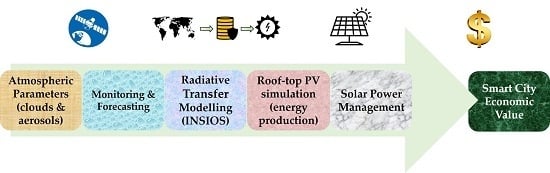
1. Introduction
2. Data and Methodology
2.1. Data
2.1.1. INSAT-3D
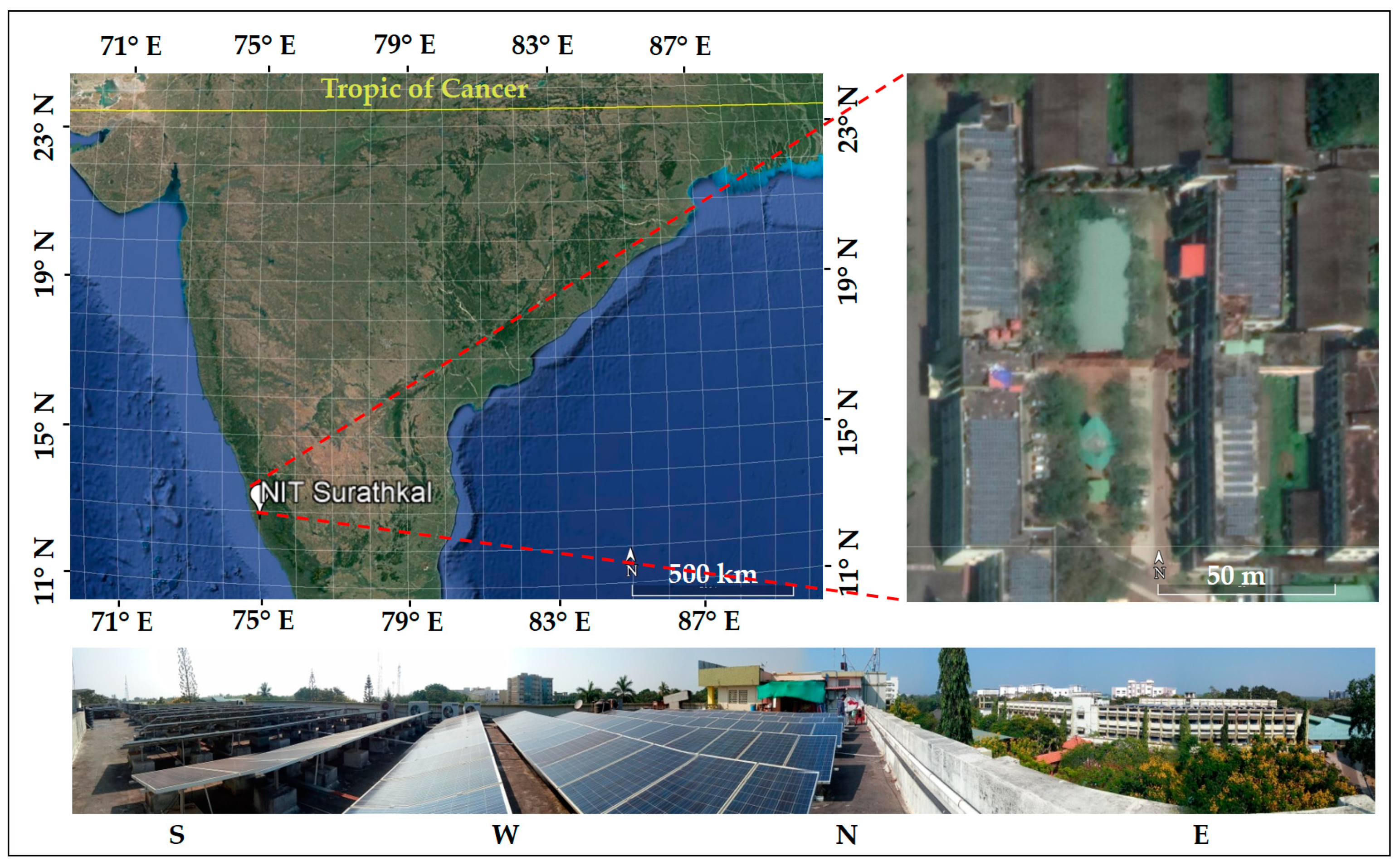
2.1.2. Rooftop PV
2.1.3. Solar Sensor
2.2. Methodology
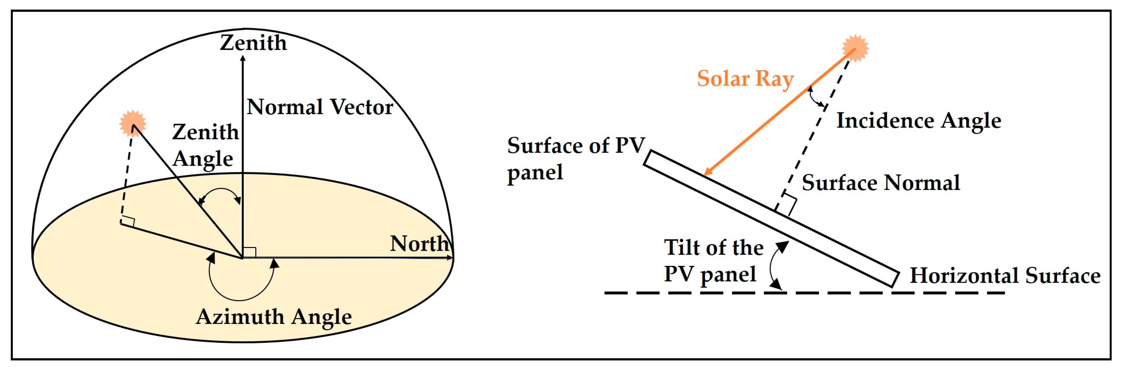
2.2.1. Solar Irradiance Simulation (INSIOS)
2.2.2. Energy Production Calculation
2.2.3. Assumptions
3. Result
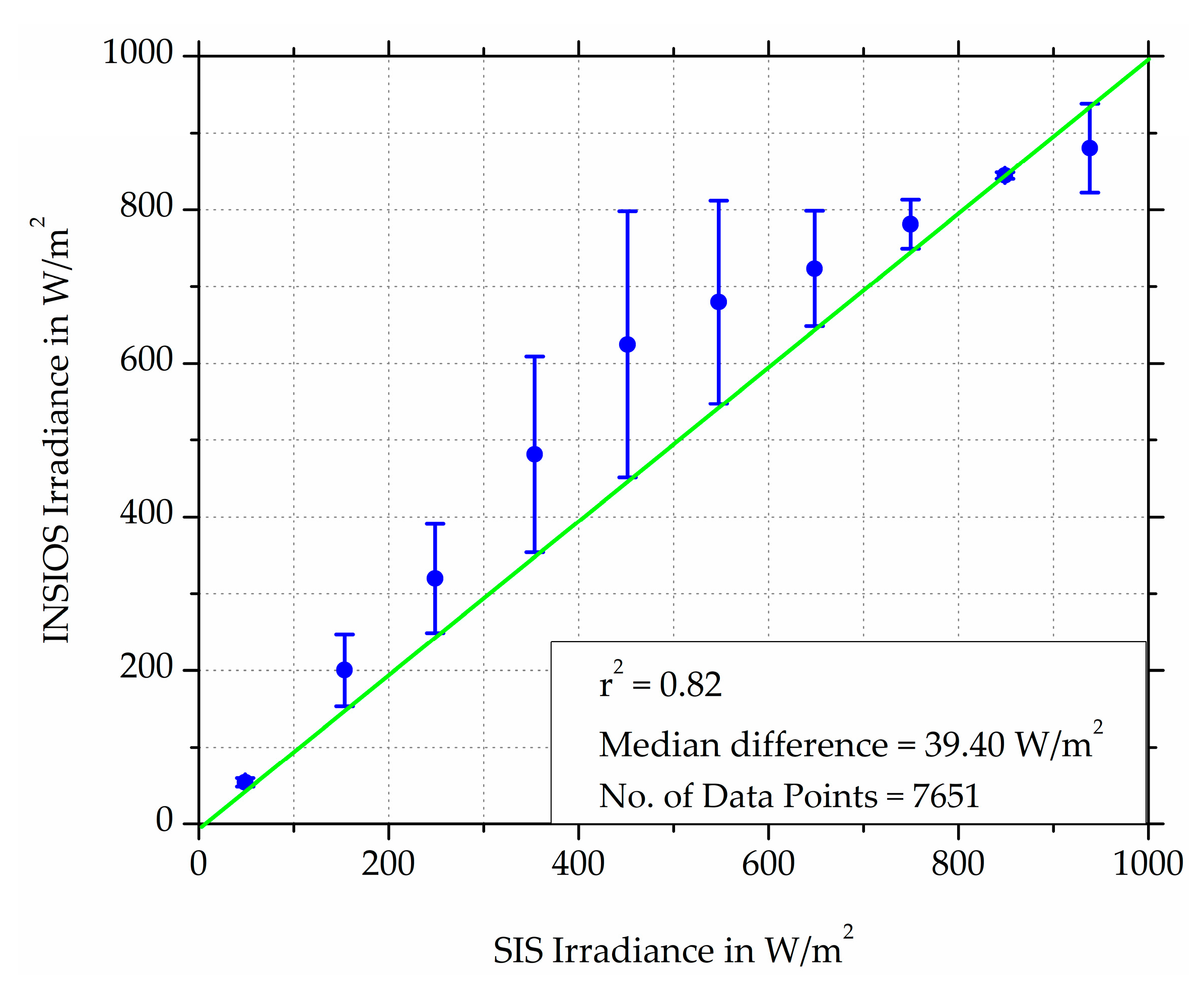
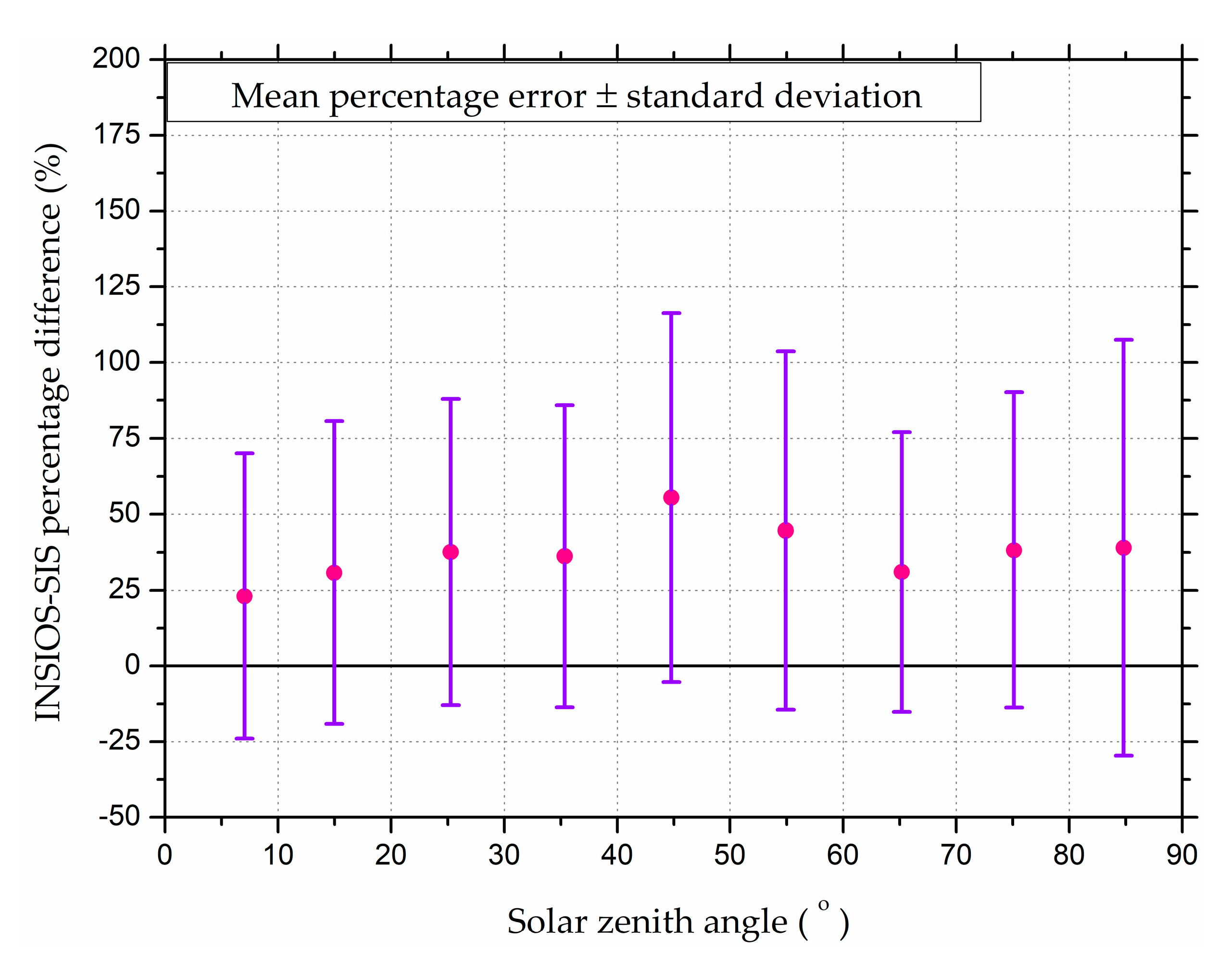
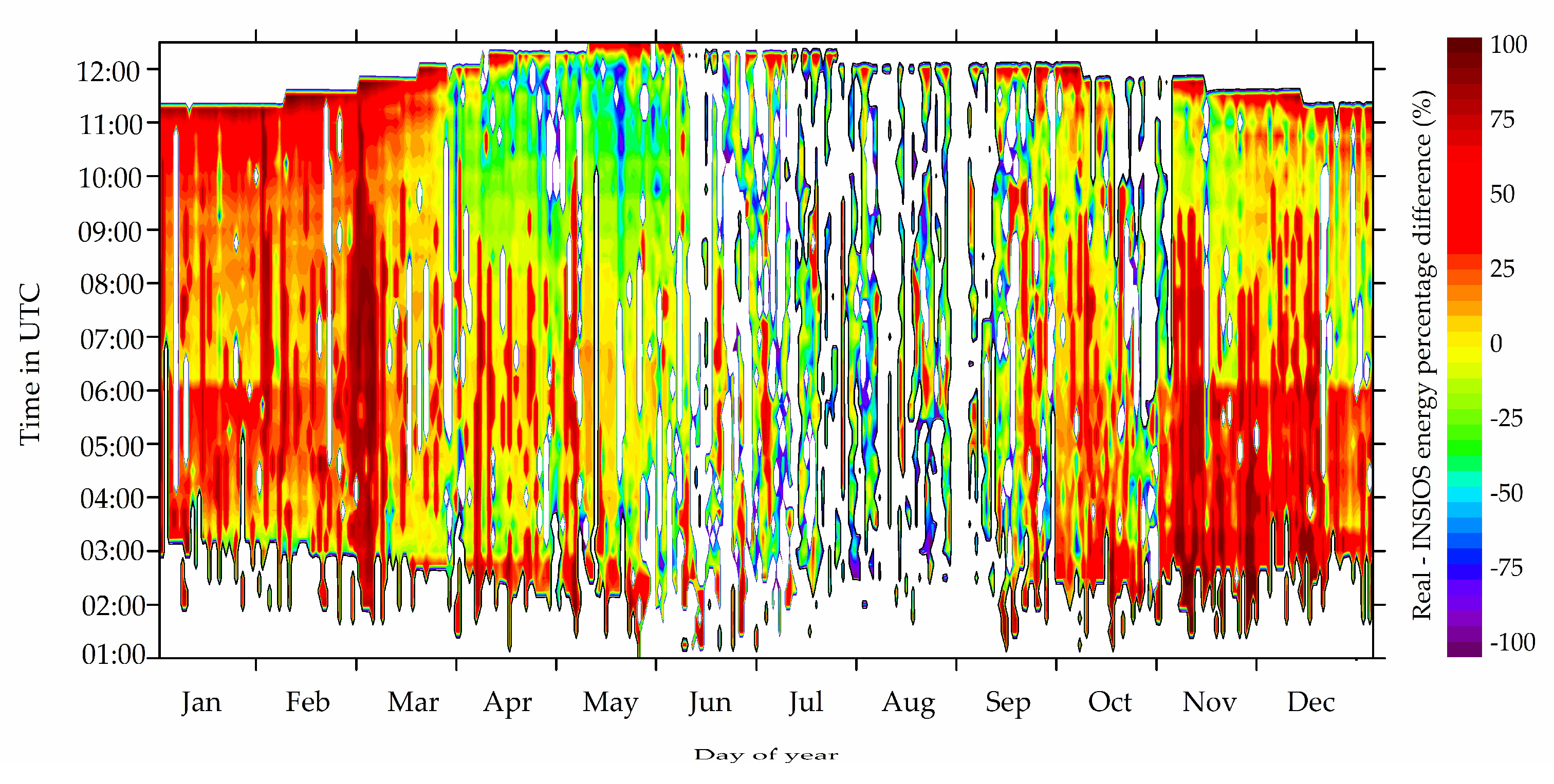
3.1. Comparison of Solar Irradiance (INSIOS vs. SIS)
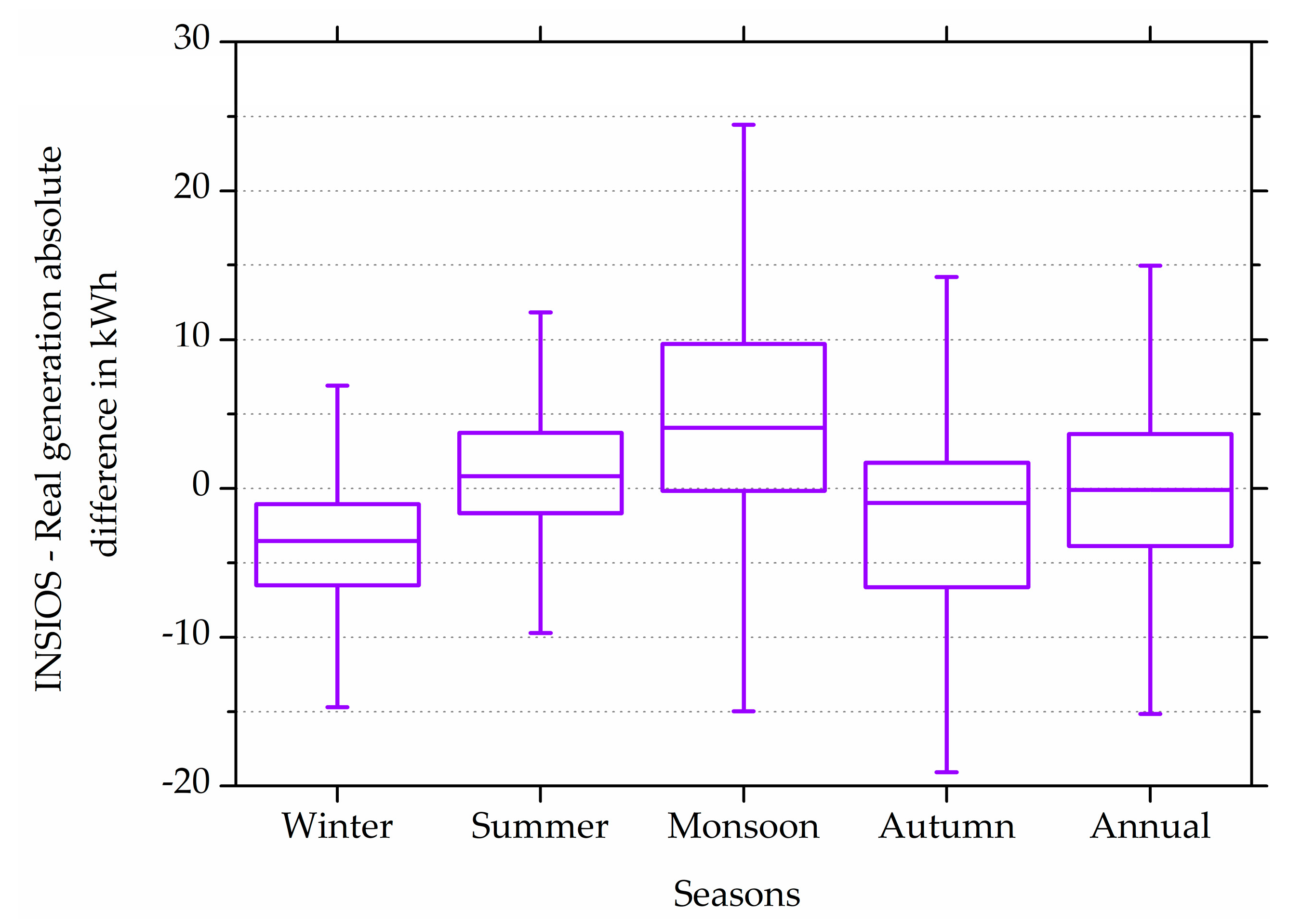
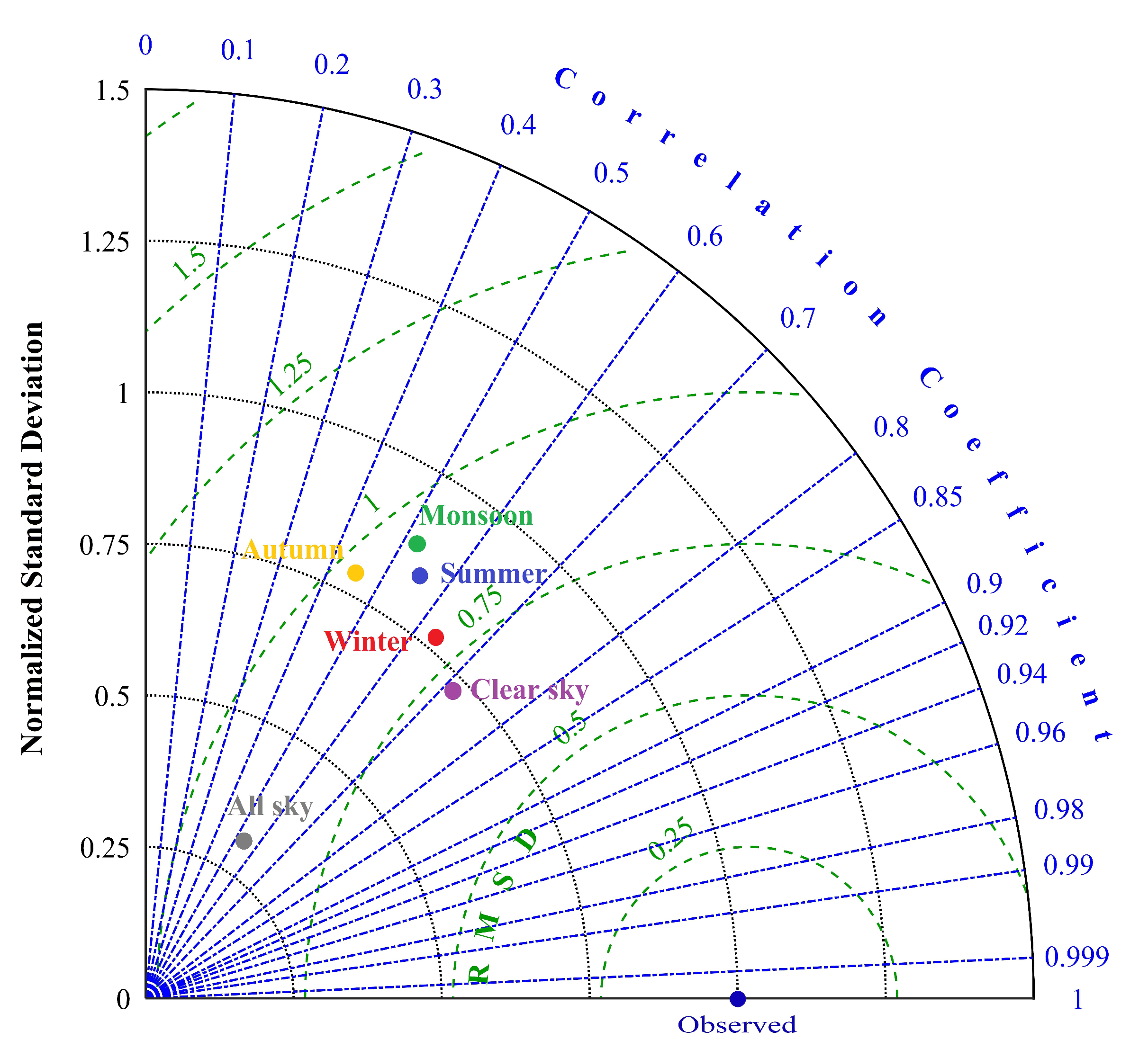
3.2. Reliability of Energy Production Estimations
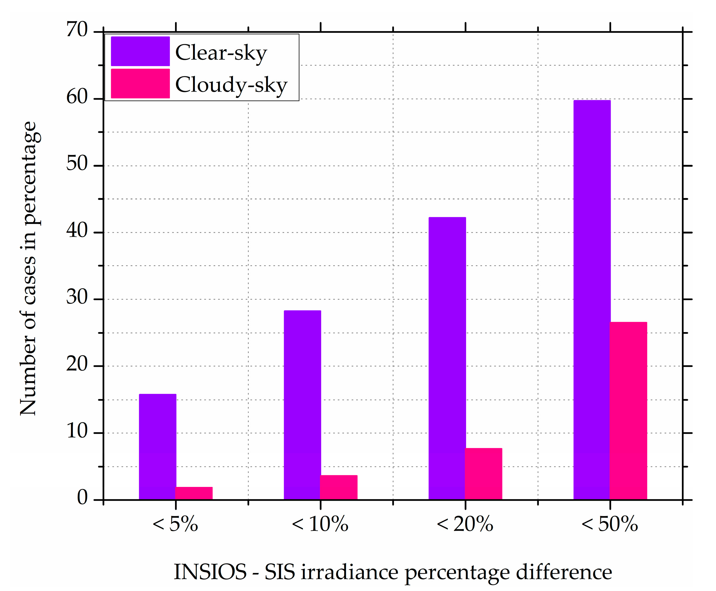
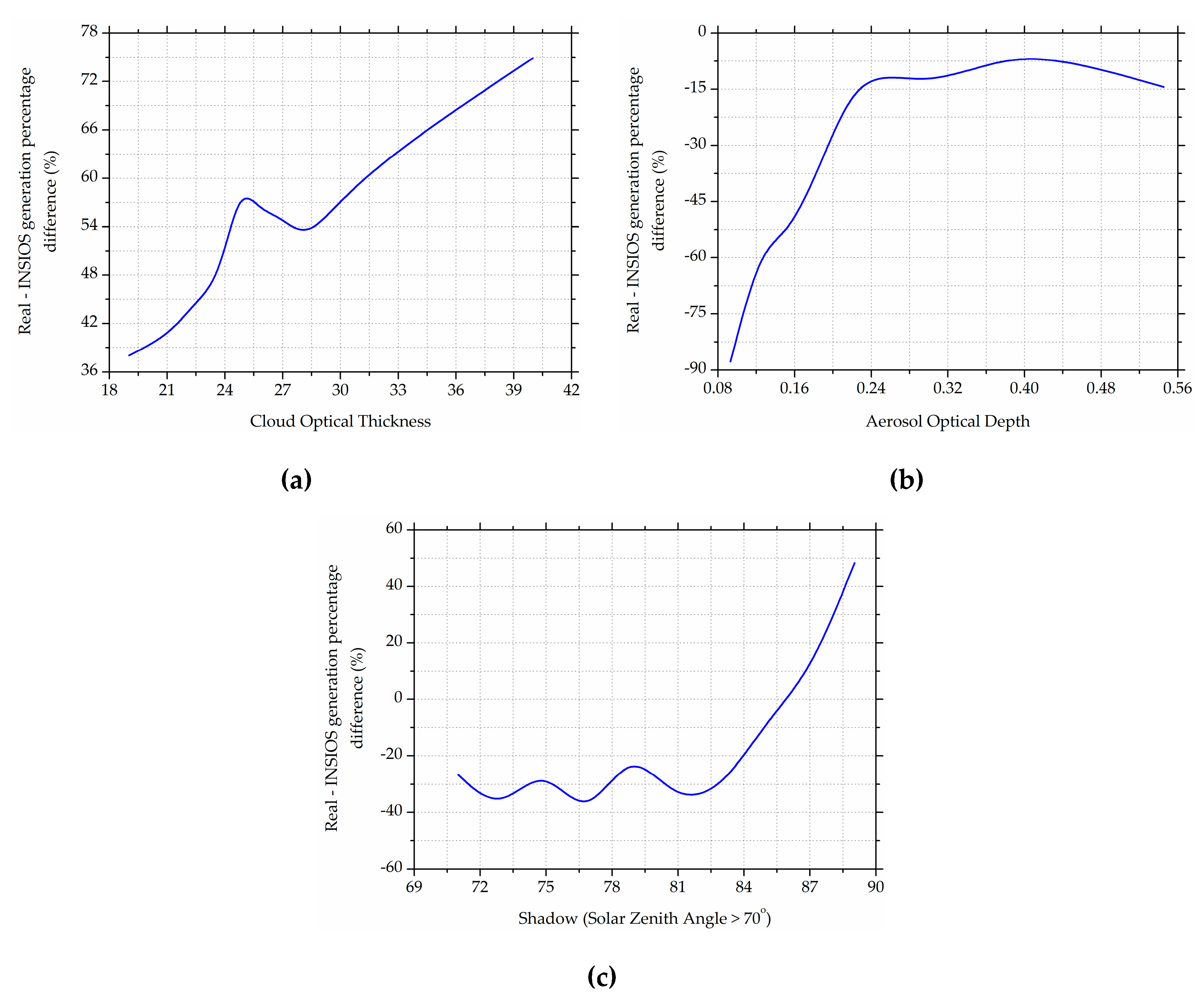
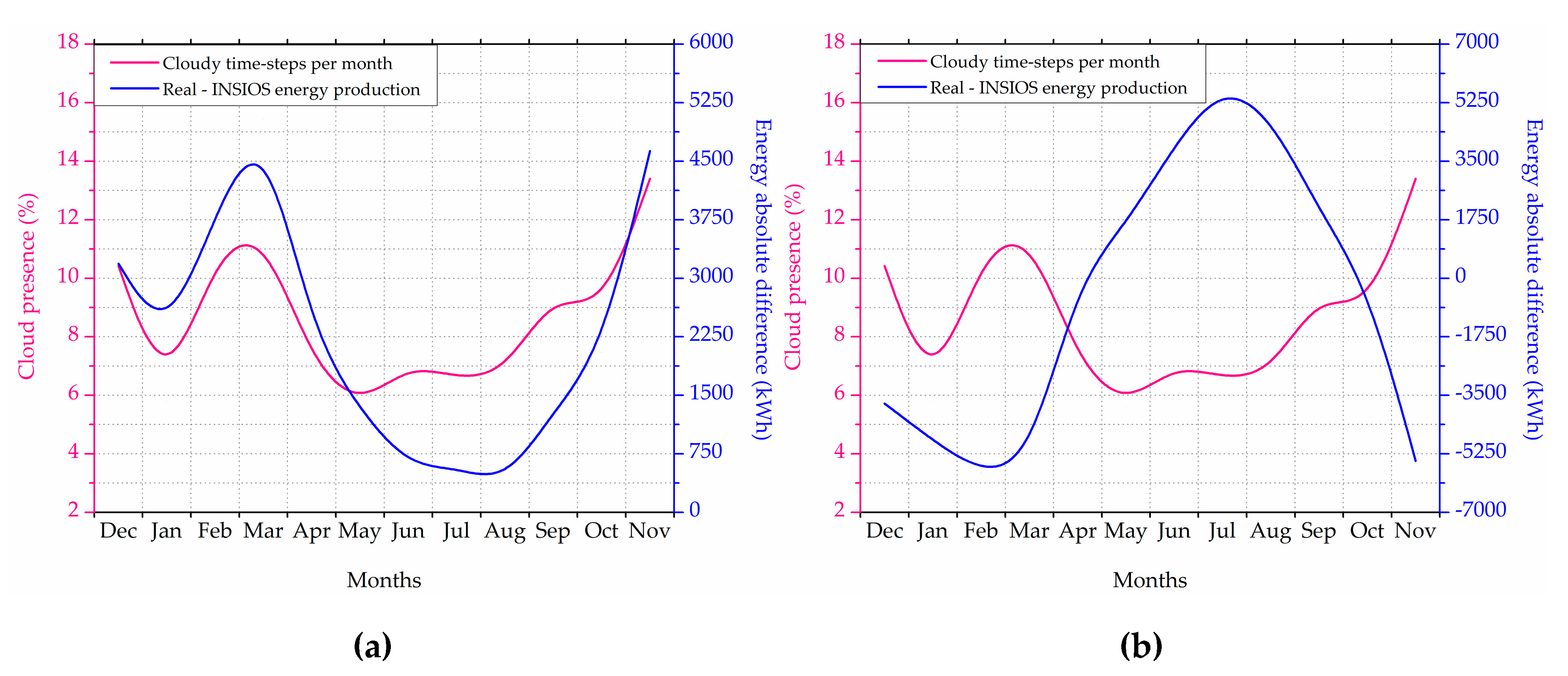
3.3. Cloud and Shadow Effect
4. Discussions
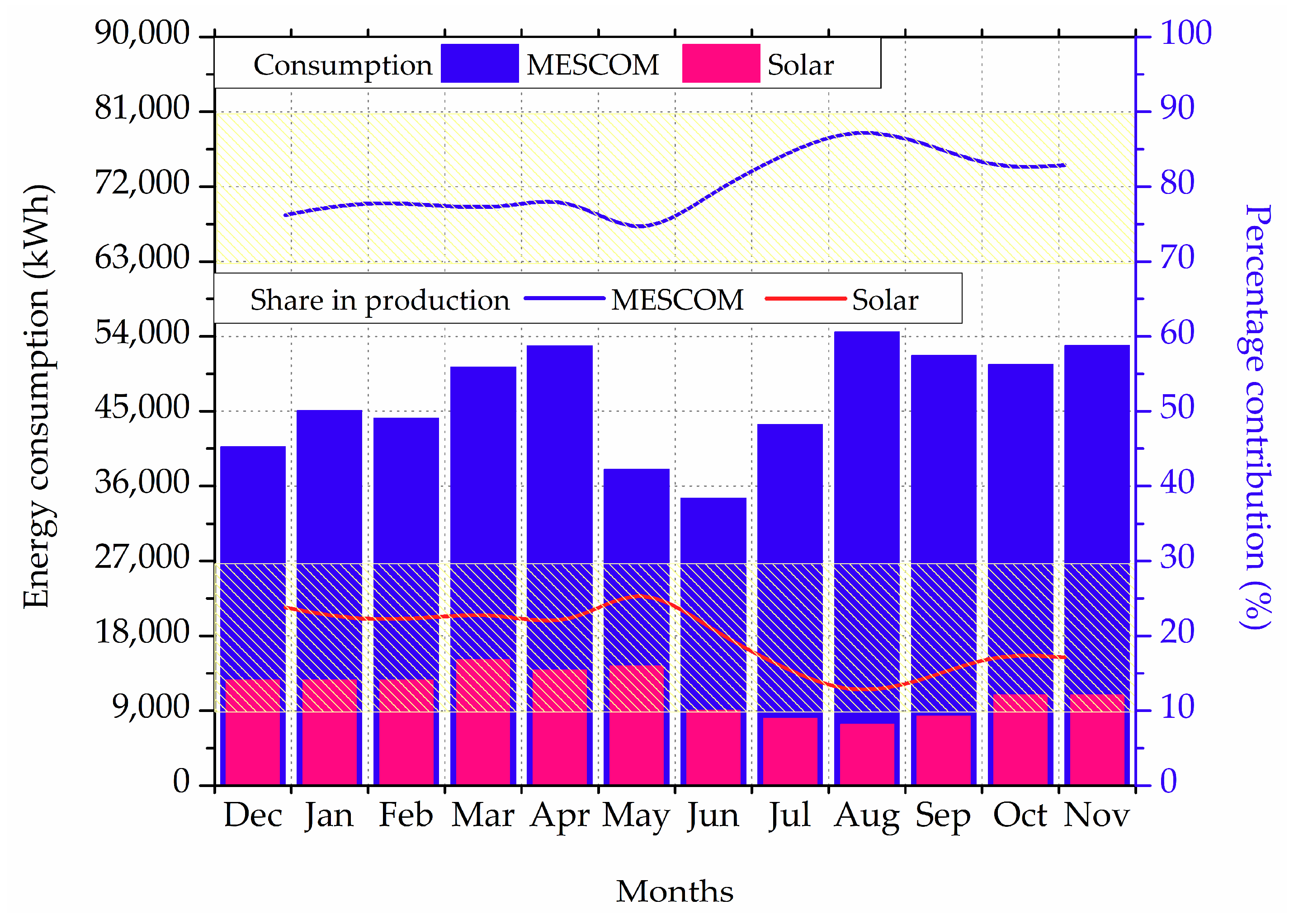
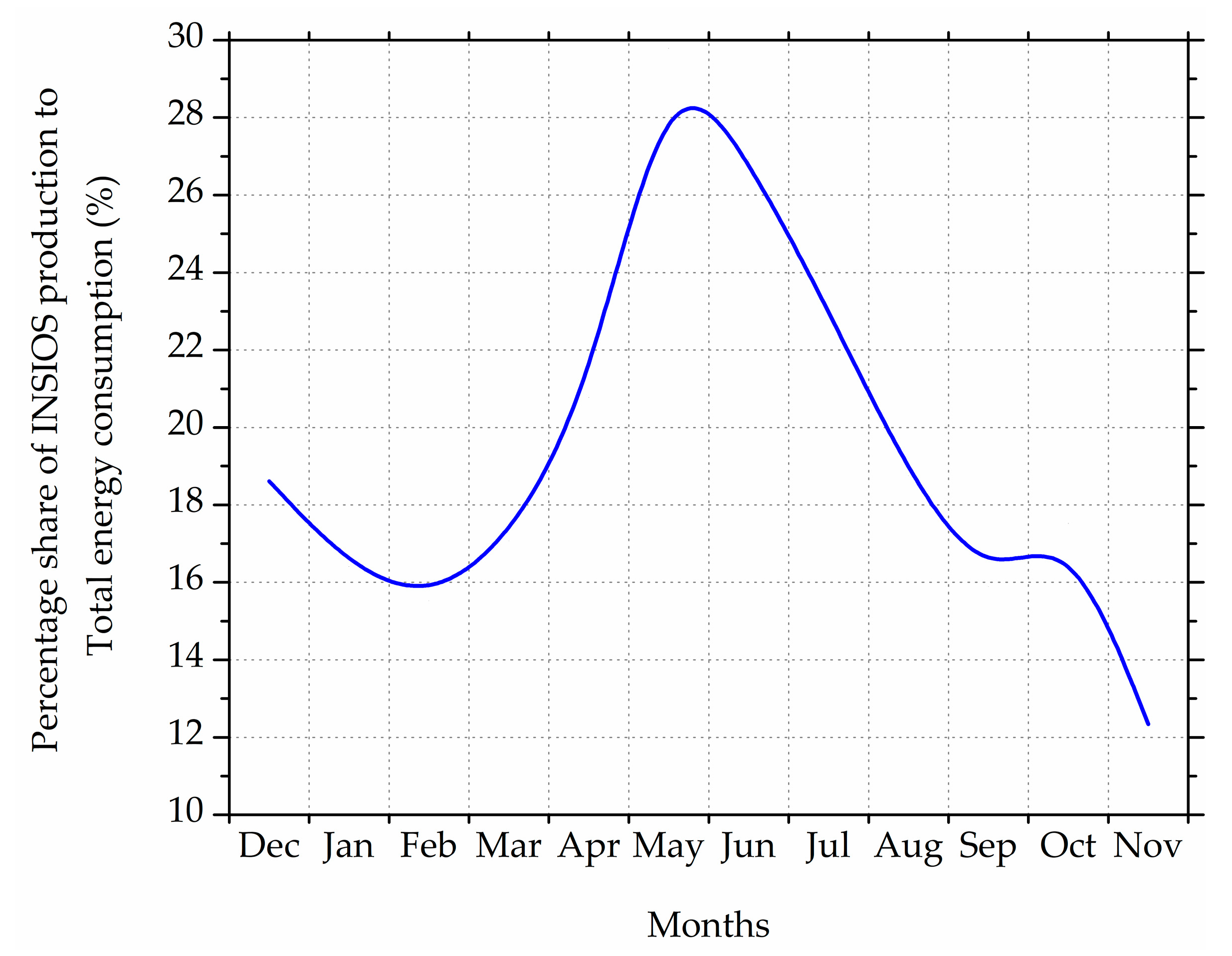
4.1. PV Energy Production Management
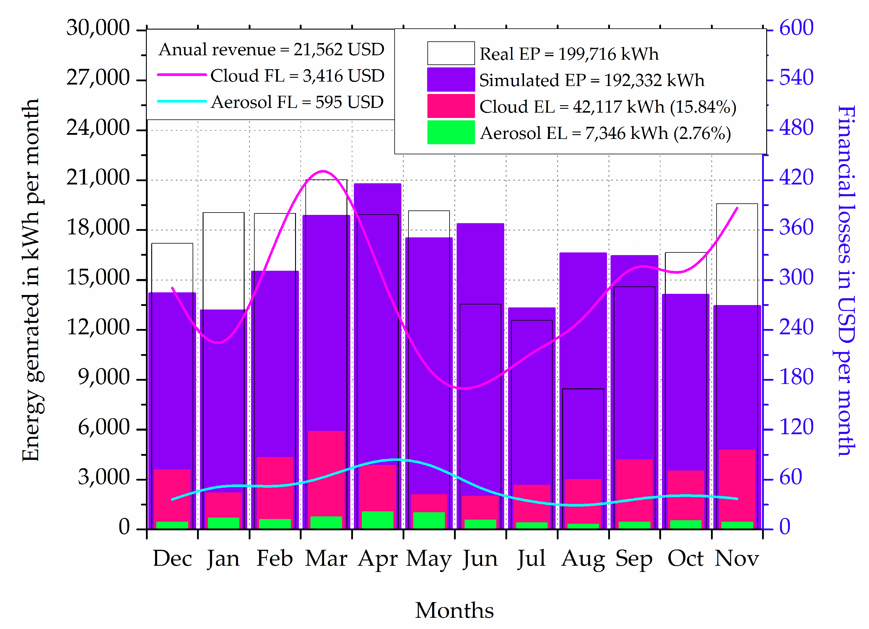
4.2. Financial Analysis (Economic Impact of Cloud and Aerosol Uncertainty)
5. Conclusions
Author Contributions
Funding
Acknowledgments
Conflicts of Interest
References
- Ellabban, O.; Abu-Rub, H.; Blaabjerg, F. Renewable energy resources: Current status, future prospects and their enabling technology. Renew. Sustain. Energy Rev. 2014, 39, 748–764. [Google Scholar] [CrossRef]
- Gielen, D.; Saygin, D.; Wagner, N.; Ghosh, A.; Chawla, K. Renewable Energy Prospects for India, a Working Paper Based on REmap; International Renewable Energy Agency: Abu Dhabi, UAE, 2017. [Google Scholar]
- Transmission Plan for Envisaged Renewable Capacity. Green Energy Corridor Report Vol-1; Power Grid Corporation of India Ltd.: Gurgaon, India, 2012.
- Commercial Real Estate India. India 2030 Exploring the Future; Commercial Real Estate India: New Delhi, India, 2019. [Google Scholar]
- Anuta, A.; Ralon, P.; Taylor, M. Renewable Power Generation Costs in 2018; International Renewable Energy Agency: Abu Dhabi, UAE, 2018. [Google Scholar]
- Behuria, P. The politics of late late development in renewable energy sectors: Dependency and contradictory tensions in India’s National Solar Mission. World Dev. 2020, 126, 104726. [Google Scholar] [CrossRef]
- Sharma, S.; Jain, G.; Mishra, S.; Bhattacharya, B. Assessment of Roof-Top Solar Energy Potential in Proposed Smart Cities of India; Space Applications Centre: Jodhpur, India, 2017.
- Sharma, N.K.; Tiwari, P.K.; Sood, Y.R. Solar energy in India: Strategies, policies, perspectives and future potential. Renew. Sustain. Energy Rev. 2012, 16, 933–941. [Google Scholar] [CrossRef]
- Harriss-white, B.; Rohra, S.; Singh, N. Political Architecture of India’s Technology System for Solar Energy. Econ. Political Wkly. 2009, 44, 47. [Google Scholar]
- 60 Solar Cities to Be Developed across Country. Available online: https://pib.gov.in/Pressreleaseshare.aspx?PRID=1519372 (accessed on 5 April 2020).
- Pune Municipal Corporation. Reimagining Pune: Mission Smart City; Pune Municipal Corporation: Pune, India, 2015. [Google Scholar]
- Singh, G.K. Solar power generation by PV (Photovoltaic) technology: A review. Energy 2013, 53, 1–13. [Google Scholar] [CrossRef]
- Lund, H. Renewable energy strategies for sustainable development. Energy 2007, 32, 912–919. [Google Scholar] [CrossRef] [Green Version]
- Angelis-Dimakis, A.; Biberacher, M.; Dominguez, J.; Fiorese, G.; Gadocha, S.; Gnansounou, E.; Guariso, G.; Kartalidis, A.; Panichelli, L.; Pinedo, I.; et al. Methods and tools to evaluate the availability of renewable energy sources. Renew. Sustain. Energy Rev. 2011, 15, 1182–1200. [Google Scholar] [CrossRef]
- International Energy Agency. Potential for Building Integrated Photovoltaics; International Energy Agency: Paris, France, 2002. [Google Scholar]
- Gharakhani Siraki, A.; Pillay, P. Study of optimum tilt angles for solar panels in different latitudes for urban applications. Sol. Energy 2012, 86, 1920–1928. [Google Scholar] [CrossRef]
- Tiris, M.; Tiris, C. Optimum collector slope and model evaluation: Case study for Gebze, Turkey. Energy Convers. Manag. 1998, 39, 167–172. [Google Scholar] [CrossRef]
- Rowlands, I.H.; Kemery, B.P.; Beausoleil-Morrison, I. Optimal solar-PV tilt angle and azimuth: An Ontario (Canada) case-study. Energy Policy 2011, 39, 1397–1409. [Google Scholar] [CrossRef]
- El-Sebaii, A.A.; Al-Hazmi, F.S.; Al-Ghamdi, A.A.; Yaghmour, S.J. Global, direct and diffuse solar radiation on horizontal and tilted surfaces in Jeddah, Saudi Arabia. Appl. Energy 2010, 87, 568–576. [Google Scholar] [CrossRef]
- Koussa, M.; Saheb-Koussa, D.; Hamane, M.; Boussaa, Z.; Lalaoui, M.A. Effect of a Daily Flat Plate Collector Orientation Change on the Solar System Performances. In Proceedings of the 7th International Renewable Energy Congress, Hammamet, Tunisia, 2016; Available online: https://0-ieeexplore-ieee-org.brum.beds.ac.uk/document/7478942 (accessed on 5 April 2020).
- Demain, C.; Journée, M.; Bertrand, C. Evaluation of different models to estimate the global solar radiation on inclined surfaces. Renew. Energy 2013, 50, 710–721. [Google Scholar] [CrossRef]
- Ko, L.; Wang, J.C.; Chen, C.Y.; Tsai, H.Y. Evaluation of the development potential of rooftop solar photovoltaic in Taiwan. Renew. Energy 2015, 76, 582–595. [Google Scholar] [CrossRef]
- Arán Carrión, J.; Espín Estrella, A.; Aznar Dols, F.; Zamorano Toro, M.; Rodríguez, M.; Ramos Ridao, A. Environmental decision-support systems for evaluating the carrying capacity of land areas: Optimal site selection for grid-connected photovoltaic power plants. Renew. Sustain. Energy Rev. 2008, 12, 2358–2380. [Google Scholar] [CrossRef]
- Wiginton, L.K.; Nguyen, H.T.; Pearce, J.M. Quantifying rooftop solar photovoltaic potential for regional renewable energy policy. Comput. Environ. Urban Syst. 2010, 34, 345–357. [Google Scholar] [CrossRef] [Green Version]
- Mulherin, A.; Pratson, L. A Spatial Approach to Determine Solar PV Potential for Durham Homeowners; Duke University: Durham, NC, USA, 2011. [Google Scholar]
- Snow, M.; Prasad, D. Designing with Solar Power: A Source Book for Building Integrated Photovoltaics; Earthscan: London, UK, 2005; ISBN 978-1-31506-573-1. [Google Scholar] [CrossRef]
- Tooke, T.R.; Coops, N.C. A Review of Remote Sensing for Urban Energy System Management and Planning. Proceeding of the Joint Urban Remote Sensing Event, Sao Paulo, Brazil, 21–23 April 2013; pp. 167–170. [Google Scholar]
- Beyer, H.G.; Costanzo, C.; Heinemann, D. Modifications of the Heliosat procedure for irradiance estimates from satellite images. Sol. Energy 1996, 56, 207–212. [Google Scholar] [CrossRef]
- Hammer, A.; Heinemann, D.; Hoyer, C.; Kuhlemann, R.; Lorenz, E.; Müller, R.; Beyer, H.G. Solar energy assessment using remote sensing technologies. Remote Sens. Environ. 2003, 86, 423–432. [Google Scholar] [CrossRef]
- Lefèvre, M.; Oumbe, A.; Blanc, P.; Espinar, B.; Gschwind, B.; Qu, Z.; Wald, L.; Schroedter-Homscheidt, M.; Hoyer-Klick, C.; Arola, A.; et al. McClear: A new model estimating downwelling solar radiation at ground level in clear-sky conditions. Atmos. Meas. Tech. 2013, 6, 2403–2418. [Google Scholar] [CrossRef] [Green Version]
- Mueller, R.W.; Matsoukas, C.; Gratzki, A.; Behr, H.D.; Hollmann, R. The CM-SAF operational scheme for the satellite based retrieval of solar surface irradiance—A LUT based eigenvector hybrid approach. Remote Sens. Environ. 2009, 113, 1012–1024. [Google Scholar] [CrossRef]
- Huang, G.; Ma, M.; Liang, S.; Liu, S.; Li, X. A LUT-based approach to estimate surface solar irradiance by combining MODIS and MTSAT data. Geophys. Res. Atmos. 2011, 116, 1–14. [Google Scholar] [CrossRef] [Green Version]
- MODIS Web. Available online: https://modis.gsfc.nasa.gov/about/ (accessed on 26 May 2020).
- Masoom, A.; Kosmopoulos, P.; Bansal, A.; Kazadzis, S. Solar Energy Estimations in India Using Remote Sensing Technologies and Validation with Sun Photometers in Urban Areas. Remote Sens. 2020, 12, 254. [Google Scholar] [CrossRef] [Green Version]
- Mayer, B.; Kylling, A. Technical Note: The libRadtran software package for radiative transfer calculations—description and examples of use. Atmos. Chem. Phys. 2005, 5, 1855–1877. [Google Scholar] [CrossRef] [Green Version]
- Mayer, B.; Kylling, A.; Emde, C.; Buras, R.; Hamann, U.; Gasteiger, J.; Richter, B. LibRadtran User’s Guide. 2017. Available online: http://libradtran.org/doc/libRadtran.pdf (accessed on 16 March 2020).
- Kosmopoulos, P.G.; Kazadzis, S.; El-Askary, H.; Taylor, M.; Gkikas, A.; Proestakis, E.; Kontoes, C.; El-Khayat, M.M. Earth-Observation-Based Estimation and Forecasting of Particulate Matter Impact on Solar Energy in Egypt. Remote Sens. 2018, 10, 1870. [Google Scholar] [CrossRef] [Green Version]
- Evenflow SPRL. Business Plan for the Establishment, Operation and Exploitation of a Solar Farm: Aswan’s Solar Plant Project Extension of Sir Magdi Yacoub Heart Hospital; Evenflow SPRL: Aswan, Egypt, 2017. [Google Scholar]
- John, J.; Dey, I.; Pushpakar, A.; Sathiyamoorthy, V.; Shukla, B.P. INSAT-3D cloud microphysical product: Retrieval and validation. Int. J. Remote Sens. 2019, 40, 1481–1494. [Google Scholar] [CrossRef]
- National Satellite Meteorological Centre. INSAT-3D Products Catalog; India Meteorological Department: New Delhi, India, 2014.
- Meteorological & Oceanographic Satellite Data Archival Centre | Space Applications Centre, ISRO. Available online: https://www.mosdac.gov.in/ (accessed on 8 June 2019).
- Atmospheric Monitoring Service | Copernicus. Available online: https://atmosphere.copernicus.eu/data (accessed on 16 November 2019).
- Schroedter-Homscheidt, M.; Hoyer-klick, C.; Killius, N.; Lefèvre, M. User’s Guide to the CAMS Radiation Service. Copernicus Atmosphere Monitoring Service; German Aerospace Center: Cologne, Germany, 2017. [Google Scholar]
- Eissa, Y.; Korany, M.; Aoun, Y.; Boraiy, M.; Wahab, M.M.A.; Alfaro, S.C.; Blanc, P.; El-Metwally, M.; Ghedira, H.; Hungershoefer, K.; et al. Validation of the Surface Downwelling Solar Irradiance Estimates of the HelioClim-3 Database in Egypt. Remote Sens. 2015, 7, 9269–9291. [Google Scholar] [CrossRef] [Green Version]
- Copernicus Atmosphere Monitoring Service. Validation Report of the CAMS Near-Real Time Global Atmospheric Composition Service; Royal Netherlands Meteorological Institute: De Bilt, Netherlands, 2019. [Google Scholar]
- Shukla, A.K.; Sudhakar, K.; Baredar, P. Design, simulation and economic analysis of standalone roof top solar PV system in India. Sol. Energy 2016, 136, 437–449. [Google Scholar] [CrossRef]
- Cebecauer, T.; Huld, T.; Suri, M. Using High-Resolution Digital Elevation Model for Improved PV Yield Estimates. In Proceedings of the 22nd European Photovoltaic Solar Energy Conference, Milano, Italy, 3–7 September 2007; pp. 3553–3557. [Google Scholar]
- Solar Irradiance Sensors: Ingenieurbüro Mencke & Tegtmeyer GmbH. Available online: https://www.imt-solar.com/solar-irradiance-sensors/ (accessed on 19 April 2020).
- Duffee, J.A.; Bechman, W.A. Solar Energy of Thermal Processes, 4th ed.; John Wiley & Sons: Hoboken, NJ, USA, 2013; ISBN 978-04-7087-366-3. [Google Scholar] [CrossRef]
- Maleki, S.A.M.; Hizam, H.; Gomes, C. Estimation of Hourly, Daily and Monthly Global Solar Radiation on Inclined Surfaces: Models Re-Visited. Energies 2017, 10, 134. [Google Scholar] [CrossRef] [Green Version]
- Badescu, V. 3D isotropic approximation for solar diffuse irradiance on tilted surfaces. Renew. Energy 2002, 26, 221–233. [Google Scholar] [CrossRef]
- Karnataka leads Indian States in New Rooftop PV Attractiveness Index. Available online: https://list.solar/news/karnataka-leads/ (accessed on 29 May 2020).
- Kosmopoulos, P.G.; Kazadzis, S.; Taylor, M.; Raptis, P.I.; Keramitsoglou, I.; Kiranoudis, C.; Bais, A.F. Assessment of surface solar irradiance derived from real-time modelling techniques and verification with ground-based measurements. Atmos. Meas. Tech. 2017, 11, 907–924. [Google Scholar] [CrossRef] [Green Version]
- Rajput, D.S.; Sudhakar, K. Effect of Dust on the Performance of Solar PV. In Proceedings of the International Conference on Global Scenario in Environment and Energy, Bhopal, India, 14–16 March 2013; pp. 1083–1086. [Google Scholar]
- Shukla, K.N.; Rangnekar, S.; Sudhakar, K. Comparative study of isotropic and anisotropic sky models to estimate solar radiation incident on tilted surface: A case study for Bhopal India. Energy Rep. 2015, 1, 96–103. [Google Scholar] [CrossRef] [Green Version]
- Šúri, M.; Huld, T.A.; Dunlop, E.D.; Ossenbrink, H.A. Potential of solar electricity generation in the European Union member states and candidate countries. Sol. Energy 2007, 81, 1295–1305. [Google Scholar] [CrossRef]
- Eck, T.F.; Holben, B.N.; Slutsker, I.; Setzer, A.; Intercomparison, T. Measurements of irradiance attenuation and estimation of aerosol single scattering albedo for biomass burning aerosols in Amazonia. Geophys. Res. Atmos. 1998, 103, 31865–31878. [Google Scholar] [CrossRef]
- Kosmopoulos, P.G.; Kazadzis, S.; Taylor, M.; Athanasopoulou, E.; Speyer, O.; Raptis, P.I.; Marinou, E.; Proestakis, E.; Solomos, S.; Gerasopoulos, E.; et al. Dust Iimpact on surface solar irradiance assessed with model simulations, satellite observations and ground-based measurements. Atmos. Meas. Tech. 2017, 10, 2435–2453. [Google Scholar] [CrossRef] [Green Version]
- Eskes, H.; Huijnen, V.; Arola, A.; Benedictow, A.; Blechschmidt, A.M.; Botek, E.; Boucher, O.; Bouarar, I.; Chabrillat, S.; Cuevas, E.; et al. Validation of Rreactive gases and aerosols in the MACC global analysis and forecast system. Geosci. Model Dev. 2015, 8, 3523–3543. [Google Scholar] [CrossRef] [Green Version]
- Riihelä, A.; Kallio, V.; Devraj, S.; Sharma, A.; Lindfors, A.V. Validation of the SARAH-E Satellite-Based Surface Solar Radiation Estimates over India. Remote Sens. 2018, 10, 392. [Google Scholar] [CrossRef] [Green Version]
- Maghami, M.R.; Hizam, H.; Gomes, C.; Radzi, M.A.; Rezadad, M.I.; Hajighorbani, S. Power loss due to soiling on solar panel: A review. Renew. Sustain. Energy Rev. 2016, 59, 1307–1316. [Google Scholar] [CrossRef] [Green Version]
- Rieger, D.; Steiner, A.; Bachmann, V.; Gasch, P.; Förstner, J.; Deetz, K.; Vogel, B.; Vogel, H. Impact of the 4 April 2014 Saharan dust outbreak on the photovoltaic power generation in Germany. Atmos. Chem. Phys. 2017, 17, 13391–13415. [Google Scholar] [CrossRef] [Green Version]
- Neher, I.; Buchmann, T.; Crewell, S.; Evers-Dietze, B.; Pfeilsticker, K.; Pospichal, B.; Schirrmeister, C.; Meilinger, S. Impact of atmospheric aerosols on photovoltaic energy production Scenario for the Sahel zone. Energy Procedia 2017, 125, 170–179. [Google Scholar] [CrossRef]
- Solar Radiation Basics | Department of Energy. Available online: https://www.energy.gov/eere/solar/articles/solar-radiation-basics (accessed on 15 April 2020).
- Kosmopoulos, P.G.; Kazadzis, S.; Lagouvardos, K.; Kotroni, V.; Bais, A. Solar energy prediction and verification using operational model forecasts and ground-based solar measurements. Energy 2015, 93, 1918–1930. [Google Scholar] [CrossRef]
- Sengupta, M.; Gotseff, P.; Myers, D.; Stoffel, T. Performance Testing Using Silicon Devices—Analysis of Accuracy. In Proceedings of the IEEE Photovoltaic Specialists Conference, Austin, TX, USA, 3–8 June 2012. [Google Scholar]
- Driesse, A.; Zaaiman, W. Characterization of Global Irradiance Sensors for Use with PV Systems. In Proceedings of the IEEE 42nd Photovoltaic Specialists Conference, New Orleans, LA, USA, 14–19 June 2015; pp. 2–6. [Google Scholar]
- Dunlop, E.D.; Halton, D. The performance of crystalline silicon photovoltaic solar modules after 22 years of continuous outdoor exposure. Prog. Photovolt. Res. Appl. 2006, 14, 53–64. [Google Scholar] [CrossRef]
- Huld, T.; Gottschalg, R.; Beyer, H.G.; Topič, M. Mapping the performance of PV modules, effects of module type and data averaging. Sol. Energy 2010, 84, 324–338. [Google Scholar] [CrossRef]
- Huld, T.; Cebecauer, T.; Šúri, M.; Dunlop, E.D. Analysis of one-axis tracking strategies for PV systems in Europe. Prog. Photovolt. Res. Appl. 2010, 18, 183–194. [Google Scholar] [CrossRef]
- Perez, R.; Cebecauer, T.; Šúri, M. Semi-Empirical Satellite Models. In Solar Energy Forecasting and Resource Assessment, 1st ed.; Kleissl, J., Ed.; Academic Press: Cambridge, MA, USA, 2013; pp. 21–48. ISBN 978-0-1239-7772-4. [Google Scholar] [CrossRef]
- Ramachandran, S.; Kedia, S. Aerosol-Precipitation Interactions over India: Review and Future Perspectives. Adv. Meteorol. 2013, 2013, 649156. [Google Scholar] [CrossRef] [Green Version]
- Thotakura, S.; Kondamudi, S.C.; Xavier, J.F.; Quanjin, M.; Reddy, G.R.; Gangwar, P.; Davuluri, S.L. Operational performance of megawatt-scale grid integrated rooftop solar PV system in tropical wet and dry climates of India. Case Stud. Therm. Eng. 2020, 18, 100602. [Google Scholar] [CrossRef]
- Climate and Average Monthly Weather in Mangalore (Karnataka), India. Available online: https://weather-and-climate.com/average-monthly-Rainfall-Temperature-Sunshine,Mangalore,India (accessed on 1 April 2020).
- Polo, J.; Zarzalejo, L.F.; Cony, M.; Navarro, A.A.; Marchante, R.; Martín, L.; Romero, M. Solar radiation estimations over India using Meteosat satellite images. Sol. Energy 2011, 85, 2395–2406. [Google Scholar] [CrossRef]
- Dunning, C.M.; Turner, A.G.; Brayshaw, D.J. The impact of monsoon intraseasonal variability on renewable power generation in India. Environ. Res. Lett. 2015, 10, 6064002. [Google Scholar] [CrossRef]
- Sendanayake, S.; Miguntanna, N.P.; Jayasinghe, M.T.R. Predicting solar radiation for tropical islands from rainfall data. Urban Environ. Eng. 2015, 9, 109–118. [Google Scholar] [CrossRef]
- Deneke, H.M.; Feijt, A.J.; Roebeling, R.A. Estimating surface solar irradiance from METEOSAT SEVIRI-derived cloud properties. Remote Sens. Environ. 2008, 112, 3131–3141. [Google Scholar] [CrossRef]
- Perez, R.; Stewart, R.; Arbogast, C.; Seals, R.; Scott, J. An anisotropic hourly diffuse radiation model for sloping surfaces: Description, performance validation, site dependency evaluation. Sol. Energy 1986, 36, 481–497. [Google Scholar] [CrossRef]
- Desthieux, G.; Carneiro, C.; Camponovo, R.; Ineichen, P.; Morello, E.; Boulmier, A.; Abdennadher, N.; Dervey, S.; Ellert, C. Solar Energy Potential Assessment on Rooftops and Facades in Large Built Environments Based on Lidar Data, Image Processing, and Cloud Computing. Methodological Background, Application, and Validation in Geneva (Solar Cadaster). Front. Built Environ. 2018, 4. [Google Scholar] [CrossRef]
- Shiva Kumar, B.; Sudhakar, K. Performance evaluation of 10 MW grid connected solar photovoltaic power plant in India. Energy Rep. 2015, 1, 184–192. [Google Scholar] [CrossRef] [Green Version]
- Ministry of New and Renewable Energy. State Rooftop Solar Attractiveness Index; Ministry of New and Renewable Energy: New Delhi, India, 2018.
- Izquierdo, S.; Rodrigues, M.; Fueyo, N. A method for estimating the geographical distribution of the available roof surface area for large-scale photovoltaic energy-potential evaluations. Sol. Energy 2008, 82, 929–939. [Google Scholar] [CrossRef]
- Huld, T.A.; Suri, M.; Kenny, R.P.; Dunlop, E.D. Estimating PV Performance over Large Geographical Regions. In Proceedings of the Photovoltaic Specialists IEEE Conference, Lake Buena Vista, FL, USA, 3–7 January 2005; pp. 1679–1682. [Google Scholar]
- Ŝúri, M.; Hofierka, J. A New GIS-Based Solar Radiation Model and Its Application to Photovoltaic Assessments. Trans. GIS 2004, 8, 175–190. [Google Scholar] [CrossRef]


| Solar Zenith Angle | SIS Angular Correction | INSIOS Tilt Correction | |
|---|---|---|---|
| 0–360 min | 360–1440 min | ||
| 0–10 | 1.07 | 0.96 | 0.96 |
| 10–20 | 1.00 | 0.95 | 1.07 |
| 20–30 | 0.90 | 0.90 | 1.12 |
| 30–40 | 0.85 | 0.80 | 1.25 |
| 40–50 | 0.75 | 0.70 | 1.35 |
| 50–60 | 0.66 | 0.40 | 1.50 |
| 60–70 | 0.56 | 0.20 | 1.70 |
| 70–80 | 0.42 | 0.10 | 1.90 |
| 80–90 | 0.20 | 0.00 | 2.80 |
© 2020 by the authors. Licensee MDPI, Basel, Switzerland. This article is an open access article distributed under the terms and conditions of the Creative Commons Attribution (CC BY) license (http://creativecommons.org/licenses/by/4.0/).
Share and Cite
Masoom, A.; Kosmopoulos, P.; Kashyap, Y.; Kumar, S.; Bansal, A. Rooftop Photovoltaic Energy Production Management in India Using Earth-Observation Data and Modeling Techniques. Remote Sens. 2020, 12, 1921. https://0-doi-org.brum.beds.ac.uk/10.3390/rs12121921
Masoom A, Kosmopoulos P, Kashyap Y, Kumar S, Bansal A. Rooftop Photovoltaic Energy Production Management in India Using Earth-Observation Data and Modeling Techniques. Remote Sensing. 2020; 12(12):1921. https://0-doi-org.brum.beds.ac.uk/10.3390/rs12121921
Chicago/Turabian StyleMasoom, Akriti, Panagiotis Kosmopoulos, Yashwant Kashyap, Shashi Kumar, and Ankit Bansal. 2020. "Rooftop Photovoltaic Energy Production Management in India Using Earth-Observation Data and Modeling Techniques" Remote Sensing 12, no. 12: 1921. https://0-doi-org.brum.beds.ac.uk/10.3390/rs12121921