Evaluating the Performance of Sentinel-3A OLCI Land Products for Gross Primary Productivity Estimation Using AmeriFlux Data


School of Resource and Environmental Science, Wuhan University, Wuhan 430079, China
*
Author to whom correspondence should be addressed.
†
These authors contributed equally to this work.
Remote Sens. 2020, 12(12), 1927; https://0-doi-org.brum.beds.ac.uk/10.3390/rs12121927
Submission received: 18 April 2020
/
Revised: 3 June 2020
/
Accepted: 12 June 2020
/
Published: 14 June 2020
(This article belongs to the Special Issue Remote Sensing of Atmosphere and Underlying Surface Using OLCI and SLSTR on Board Sentinel-3: Calibration, Algorithms, Geophysical Products and Validation)
Abstract
:Accurate and reliable estimation of gross primary productivity (GPP) is of great significance in monitoring global carbon cycles. The fraction of absorbed photosynthetically active radiation (FAPAR) and vegetation index products of the Moderate Resolution Imaging Spectroradiometer (MODIS) are currently the most widely used data in evaluating GPP. The launch of the Ocean and Land Colour Instrument (OLCI) onboard the Sentinel-3 satellite provides the FAPAR and the OLCI Terrestrial Chlorophyll Index (OTCI) products with higher temporal resolution and smoother spatial distribution than MODIS, having the potential to monitor terrain GPP. OTCI is one of the red-edge indices and is particularly sensitive to canopy chlorophyll content related to GPP. The purpose of the study is to evaluate the performance of OLCI FAPAR and OTCI for the estimation of GPP across seven biomes in 2017–2018. To this end, OLCI FAPAR and OTCI products in combination with insitu meteorological data were first integrated into the MODIS GPP algorithm and in three OTCI-driven models to simulate GPP. The modeled GPP (GPPOLCI-FAPAR and GPPOTCI) were then compared with flux tower GPP (GPPEC) for each site. Furthermore, the GPPOLCI-FAPAR and GPP derived from the MODIS FAPAR (GPPMODIS-FAPAR) were compared. Results showed that the performance of GPPOLCI-FAPAR was varied in different sites, with the highest R2 of 0.76 and lowest R2 of 0.45. The OTCI-driven models that include APAR data exhibited a significant relationship with GPPEC for all sites, and models using only OTCI provided the most varied performance, with the relationship between GPPOTCI and GPPEC from strong to nonsignificant. Moreover, GPPOLCI-FAPAR (R2 = 0.55) performed better than GPPMODIS-FAPAR (R2 = 0.44) across all biomes. These results demonstrate the potential of OLCI FAPAR and OTCI products in GPP estimation, and they also provide the basis for their combination with the soon-to-launch Fluorescence Explorer satellite and their integration with the Sentinel-3 land surface temperature product into light use models for GPP monitoring at regional and global scales.
1. Introduction
Terrestrial gross primary production (GPP), which is the total amount of organic carbon fixed by green plants through photosynthesis at an ecosystem scale, determines the initial amount of energy and material entering the terrestrial ecosystem [1,2]. Terrestrial ecosystems can partly mitigate global warming and offset increasing CO2 emissions through GPP [3]. Therefore, accurately quantifying GPP is essential for assessing global climate variation and carbon cycles [4].
The eddy covariance (EC) technique is the most accurate approach to measure the net CO2 exchange (NEE) between the atmosphere and the terrestrial ecosystem [5]. NEE then partitions into ecosystem respiration and GPP using different modeling methods. However, EC provides a limited carbon flux measurements scope, ranging from a hundred meters to several kilometers around the flux tower depending on the height of the tower, canopy characteristics, wind velocity, and homogeneity of the fetch [6,7]. This limitation necessitates upscaling flux tower data to regional, continental, or global scales to reflect terrestrial carbon cycling [8].
Satellite remote sensing (RS) provides a potentially viable tool for upscaling efforts. This technology has played an increasing role in the estimation of GPP that can offset the restricted coverage of flux tower observations [9,10]. A number of RS-based models have been developed to quantify the GPP of terrestrial ecosystems because they are relatively simple and efficient [11,12,13]. The prevalent RS-based GPP models can be categorized into four groups [14]: light use efficiency (LUE) models [15,16], vegetation index (VI) driven models [17,18], process-based models [13], and machine learning models [19,20]. In the aforementioned models, LUE and VI-driven models have been most frequently used on account of their simple conceptual algorithm and practicality [21]. Therefore, only LUE and VI-driven models are discussed in this study.
The foundation of LUE models is based on the LUE concept proposed by Monteith [22], which is determined as the ratio of GPP to absorbed photosynthetically active radiation (APAR). APAR is defined as the product of photosynthetically active radiation (PAR) and the fraction of absorbed photosynthetically active radiation (FAPAR). LUE is regulated under environmental stresses such as temperature stress and water availability [23]. Without environmental stress conditions, maximal LUE (εmax) is specified for different biome types. Under environmental stresses, the εmax is down-regulated by scalars (ƒ), which varies from 0 to 1 and which represents the reduction of LUE relative to εmax due to environmental stresses. The definitions of the scalars (ƒ) are various in different LUE models [24]. Numerous LUE models have been proposed, including the Carnegie–Ames–Stanford approach (CASA) [1], the global production efficiency model (GLO-PEM) [25], the moderate resolution imaging spectroradiometer GPP algorithm (MODIS GPP) [10], the vegetation photosynthesis model (VPM) [16,26], and the eddy covariancelight use efficiency (EC-LUE) model [12]. At present, the first operational, near-real-time GPP dataset, which is based on the MODIS GPP algorithm, is the MOD17 product at an eight-day interval [27]. The primary input data of the MOD17 product are the FAPAR product (MOD15) and meteorological data. Three collections of the MOD17 GPP product (5.0, 5.5, and 6.0) are currently freely available to users. The essential improvement of the latest collection 6.0 is focused on the spatial resolution of the FAPAR (MOD15A2H) and GPP (MOD17A2H) products from 1000 to 500 m compared with the previous collections [28]. Although the MOD17 GPP products have been widely used as the recognized standard global GPP products, some discrepancies between this product and insitu measured GPP remain [29,30,31,32]. Among the problems are the uncertainties in FAPAR estimates [28,33,34]. The maximum FAPAR across the eight days is selected to represent the final FAPAR value for this period in MOD15 [35], which means FAPAR does not vary during a given eight-day period.
VI-driven models estimate GPP based on the empirical relationship between VIs and FAPAR [36]. A number of prevalent VI-driven models include the temperature and greenness (TG) model [18], the greenness and radiation (GR) model [17], and the vegetation index (VI) model [37]. The Normalized Difference Vegetation Index (NDVI) and the Enhanced Vegetation Index (EVI) are the most widely used VIs in VI-based models [38]. In addition to the NDVI and EVI, numerous studies have utilized vegetation red-edge reflectance VIs to improve GPP estimation [39,40]. The Medium Resolution Imaging Spectrometer (MERIS) Terrestrial Chlorophyll Index (MTCI), originally derived from the MERIS onboard the Envisat satellite of the European Space Agency (ESA), is one of the red-edge VIs [41]. The global MTCI product, with a spatial resolution of 1km, was available either weekly or monthly [42]. The MTCI has demonstrated its suitability to evaluate GPP across different biomes such as grasslands [43], deciduous forest, and croplands [44]. Harris and Dash [44] concluded that the MTCI performed better than the MODIS EVI products for estimating GPP across a diversity of ecosystems and climatic conditions. The MTCI product was discontinued in 2012, but the successful launch of the Ocean and Land Colour Instrument (OLCI) onboard the Sentinel-3 satellite provides the continuity of the MERIS.
As a legacy of the MERIS, the Sentinel-3 OLCI has recognized the pivotal deficiencies of MERIS and has undergone many enhancements [45]. The double satellite system of the OLCI instruments (i.e., Sentinel-3A and 3B) enables a revisit period less than two days, and 21 spectral bands exist with wavelengths ranging from optical to near-infrared in OLCI [46]. There are mainly two OLCI products levels, i.e., level-1B and level-2 (land and water), with a spatial resolution of approximately 300 m or 1.2 km. Specifically, the OLCI level-2 land products include the FAPAR and OTCI products, named the OLCI Global Vegetation Index (OGVI) and the OLCI Terrestrial Chlorophyll Index (OTCI), respectively. OGVI and OTCI are the continuity of the MERIS FAPAR (MERIS Global Vegetation Index (MGVI)) and the MTCI datasets, respectively [47]. The apparent difference of the OLCI products compared with MODIS and MERIS is the data composition algorithm. OGVI and OTCI used the actual value for the day while MOD15 and MTCI were composited using the arithmetic mean and maximum value across eight days, respectively [48]. The fine temporal and spectral resolution of OLCI products opened opportunities for GPP estimation. Nevertheless, to the best of our knowledge, only Zhang et al. [49] focused on GPP estimation using the OLCI FAPAR product so far. The main objective of their study was to investigate the relationships between a series of satellite FAPAR products (including OLCI FAPAR) and solar-induced chlorophyll fluorescence (SIF) products. Only the relationship between APAR and flux-tower based GPP was established, and neither LUE nor VI-driven models were used.
The main objective of this research is to assess the performance of the Sentinel-3 OLCI FAPAR and OTCI products in estimating GPP across different biome types. Thus, this study aims to (1) evaluate the GPP obtained from the OLCI FAPAR and three OTCI-driven models, (2) compare these obtained values of GPP with those derived from EC measurements, and (3) compare the performance between the OLCI FAPAR and MODIS FAPAR products.
2. Materials and Methods
2.1. Study Sites Description
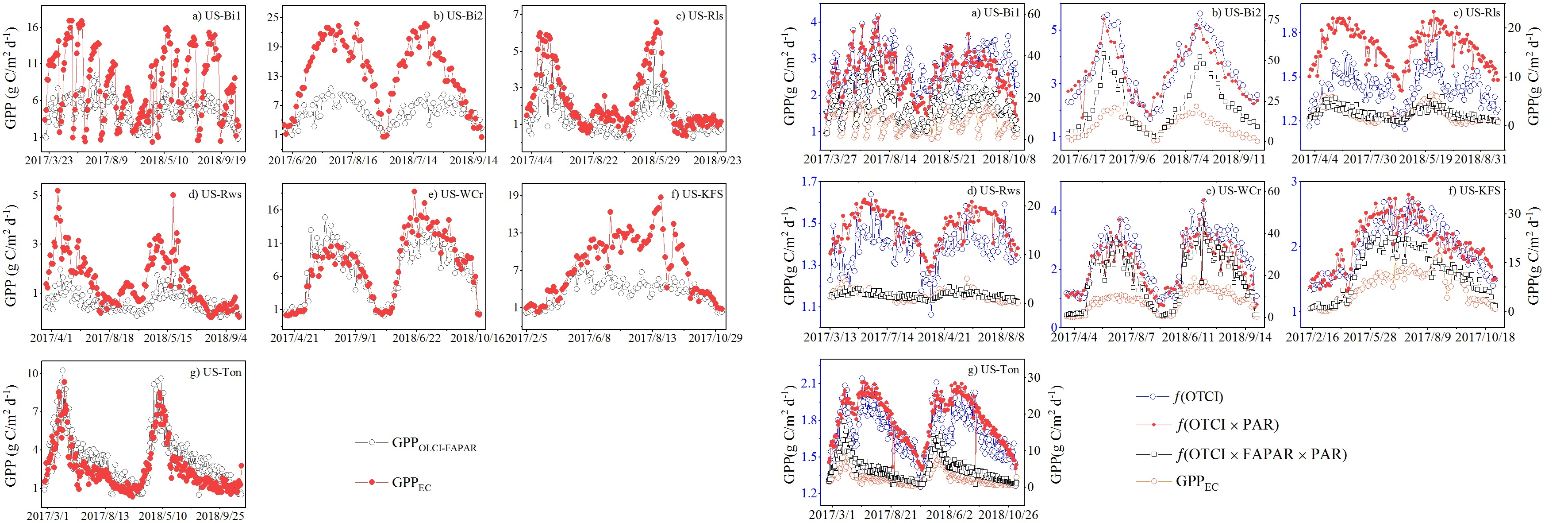
Seven AmeriFlux eddy covariance flux towers including a variety of vegetation ecosystems types with latitudes ranging from 38° to 45°N and longitudes from −122° to −89°W were selected for this study (Figure 1). These sites cover a range of climate conditions and land use classes, including two cropland (CRO) sites (C3: alfalfa and C4: corn, respectively), one grassland (GRA) site, one deciduous broadleaf forest (DBF) site, one closed shrubland (CSH) site, one open shrubland (OSH) site, and one woody savanna (WSA) site (Table 1). The reason that we selected these sites was mainly in terms of the availability of satellite images, GPP measurements, and meteorological observations data. Detailed site descriptions and other related information can be obtained via the AmeriFluxwebsite (https://ameriflux.lbl.gov/sites/site-search/).
2.2. Flux and Meteorological Data
The fluxes and meteorological data at a half-hourly scale are provided by AmeriFlux website. The AmeriFlux network provides continuous observations of CO2, water, and energy fluxes at the ecosystem and landscape levels. It also provides standard datasets of climate and CO2 fluxes to the public, after various levels of data processing have been completed. Individualsite data were standardized and rigorously quality-filtered according to established standards within AmeriFlux [54]. The data of the seven flux towers, including GPP (g C m−2 d−1), vapor pressure deficit (VPD, hPa), air temperature (Ta, °C), sensible heat (H, W m−2), downward shortwave radiation (W m−2), and latent heat (LE, W m−2), were used in our study. The daily GPP and downward shortwave radiation were calculated as the sum of the half-hourly GPP and downward shortwave radiation. The half-hourly VPD was averaged to obtain the daily VPD. The daily minimum Ta was derived from the minimum half-hourly Ta. Specifically, at the corn site, the GPP and the meteorological data only during the growing season were used to preclude the possible disturbance caused by satellite observations during the nongrowing season [55].
2.3. Satellite Products
2.3.1. Sentinel-3 OLCI Land Products
There are three processing levels (i.e., level-0, level-1, and level-2) of OLCI with various data products. OLCI level-1 and 2 data products are freely available to the general public. Products are delivered in full resolution (FR, 300 m) and reduced resolution (RR, 1.2 km) for the same coverage area. The two OLCI level-2 land products of FAPAR and OTCI at FR were used in our study.
OLCI FAPAR is essential for studying the plant photosynthetic process. The OLCI FAPAR algorithm consists of two steps. First, thebidirectional reflectance factors are “rectified”, that is, angular effects are removed. Then, the information from the blue channel is used to decontaminate the red and near-infrared bands from any atmospheric influence. Such an approach does not require any assumption on the ambient atmospheric properties [56]. Seasonality comparisons against ground-based measurements have shown that OLCI FAPAR effectively describesthe seasonal changes over various types of crops, and more ground-truth is under collection for validation purposes.
OTCI is an indicator of canopy chlorophyll content and is a continuation of the MTCI. The formula of OTCI is as follows:
where Band12, Band11, and Band10 are the reflectance in the band centered respectively at 753, 709, and 681 nm of the OLCI sensor. OTCI is easily calculated and strongly correlated with the red-edge position (REP). It is more sensitive to the high chlorophyll content compared to REP [41]. Information on canopy chlorophyll content is an important indication of plant photosynthetic capacity. OTCI ranges from 1 to 6.5. Further validation work of OTCI with additional in situ data is currently performed.
All of the Sentinel-3 OLCI products in this study were downloaded from the ESA (https://scihub.copernicus.eu). The data preprocessing operations include reprojection, resampling and subset; these batch processing operations were accomplished through the ENVI Modeler tool in ENVI 5.5.
2.3.2. MODIS FAPAR Product
Different series of MODIS FAPAR products have been widely used in modeling GPP. The latest version is Collection 6 (C6) MOD15A2H, which is composited at an eight-day interval with a spatial resolution of 500 m. The main retrieval method is based on the 3-D radiative transfer (RT) model setting canopy spectral properties for a given biome type [49]. A Look-up-Table (LUT), which is generated by 3-D RT, is used to retrieve FAPAR [57]. A back-up method based on the statistical relationships between NDVI and FAPAR is chosen as an alternative when the main RT retrieval method fails [58].
2.4. Methods
2.4.1. MODIS GPP Algorithm
In this study, we adopted the MODIS GPP algorithm combined with the Sentinel-3 OLCI FAPAR product to calculate GPP so that the result is comparable with the GPP derived from MODIS FAPAR. The MODIS GPP is a representative LUE model algorithm that calculates GPP by employing the amount of PAR absorbed by vegetation [59]. The algorithm is developed as follows:
where εmax represents the maximum LUE, TMINmin is the daily minimum temperature (Tmin) at which ε = 0, TMINmax is the daily Tmin at which ε = εmax, VPDmax is the daylight average VPD at which ε = εmax, VPDmin is the daylight average VPD at which ε = 0, FAPAR is from the OLCI FAPAR product (OGVI), and SWrad is the incident solar shortwave radiation. Here, εmax, TMINmin, TMINmax, VPDmax, and VPDmin were determined according to the biome properties LUT for each biome types (Table 2), while Tmin, VPD, and SWrad were obtained from flux tower sites. Additionally, a 1.5 km × 1.5 km area centered on every flux tower site was extracted to represent the flux footprint, FAPAR, and OTCI [5].
2.4.2. Modeling of OTCI-Driven Models
Three types of OTCI-driven models in combination with different input variables were established. Model 1 used the OTCI alone to estimate the GPP directly (GPP = ƒ (OTCI)), according to the fact that GPP is directly related to chlorophyll content, which is also closely associated with OTCI. Therefore, OTCI is regarded as a proxy for LUE and APAR [60]. Model 2 combines OTCI and the incoming shortwave radiation that uses wavelength in the 400–700 nm region to estimate GPP (GPP = ƒ (OTCI × PAR)), according to Yoder and Waring [61], who assumed a direct linear relationship between GPP and the product of photosynthetic efficiency and incoming shortwave radiation over a period of the growing season. Therefore, OTCI related to canopy chlorophyll content represents the photosynthetic efficiency here. Model 3 (GPP = ƒ (OTCI × PAR × FAPAR)) introduces the actual incoming shortwave radiation by considering only absorbed PAR (APAR = PAR × FAPAR) to be functioning for photosynthesis. Therefore, this model theoretically overcomes the limitation of the previous two models and is expected to obtain the highest potential for GPP simulation.
2.4.3. Statistical Analysis
To make a comparisonwith the GPPOLCI-FAPAR, the eight-day period of the MODIS FAPAR product was first averaged to obtain the daily value for the FAPAR. Then, the daily GPPMODIS-FAPAR was calculated based on the site meteorological data and the MODIS GPP algorithm. The GPPMODIS-FAPAR values with dates corresponding to GPPOLCI-FAPAR were selected. Moreover, it is well known that GPPEC encompasses many uncertainties. In this study, random uncertainties in GPPEC were estimated following Richardson and Hollinger [62]. Uncertaintiesare expressed as a 95% confidence interval estimated from the 2.5th and 97.5th percentiles of the daily sum in g C m−2 d−1. Three statistical metrics were used to evaluate the accuracies ofthe modeled GPP, including the coefficient of determination (R2), root mean square error (RMSE), and bias. A higher R2 and a lower RMSE and bias mean a better model performance. The RMSE and bias are calculated as follows:
where Mi and Ei are the modeled and EC-measured GPP values, respectively.
3. Results
3.1. Variability of Tmin, VPD, GPPEC, and Input Model Variables
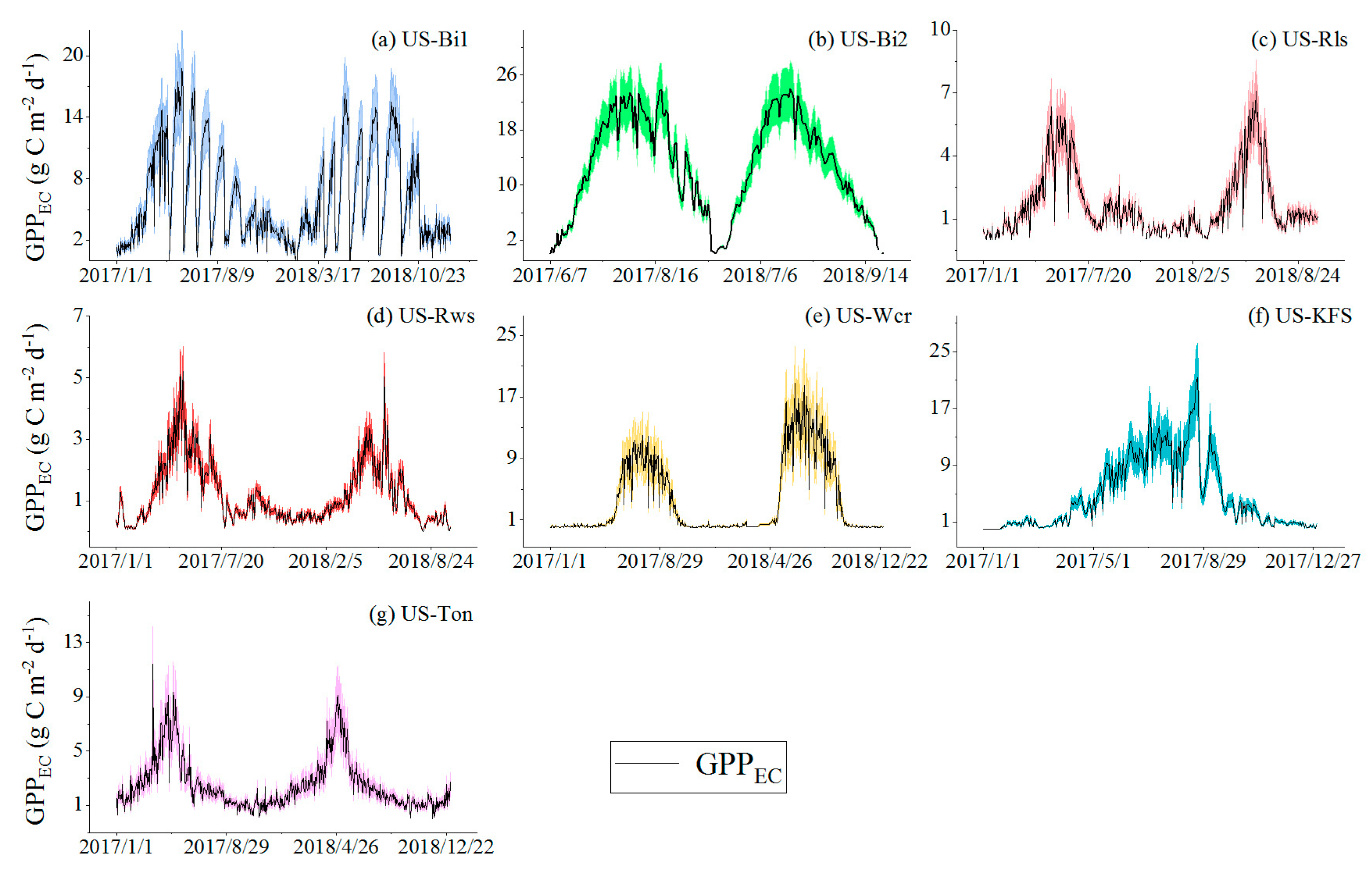
The flux-tower based GPP varied among the study sites and land use classes. The CRO sites of US-Bi2 and US-Bi1 showed the highest average GPPEC: 12.69 ± 7.04 g C m−2 d−1 at US-Bi2 and 6.11 ± 4.51g C m−2 d−1 at US-Bi1. The GRA, DBF and WSA sites showed a relatively lower average GPPEC: 4.72 ± 1.88g C m−2 d−1 at US-KFS, 3.53 ± 4.80 g C m−2 d−1 at US-WCr, and 2.54 ± 1.88 g C m−2 d−1 at US-Ton. Two types of shrubland (i.e., CSH and OSH) sites, Rls and Rws, had the lowest average GPPEC of 1.68 ± 1.59 g C m−2 d−1 and 1.21 ± 0.99 g C m−2 d−1, respectively. The temporal dynamics in GPPEC at the seven sites is shown in Figure 2. Apparently, the seasonal change patterns in the GPPEC of alfalfa and corn are different. The corn site (US-Bi2) is a single croppingsystem, whereas the alfalfa site (US-Bi1) is a multiple cropping system. At the US-Bi2 site, GPPEC rose rapidly and peaked in early August 2017 and late July 2018, respectively. At the US-Bi1 site, the harvest cycle of alfalfa is approximately a month. Alfalfa is harvested multiple times per growing season, depending on the level of rainfall and magnitude of production. Moreover, the maximum GPPEC of corn was found to be substantially larger than that of alfalfa. For example, in 2018, the highest GPPEC of corn was 23.75 ± 4.02 g C m−2 d−1, whereas alfalfa was only 16.33 ± 3.46 g C m−2 d−1. The OSH and CSH presented a similar temporal variation characteristic, reaching a peak in early May 2017 and the end of May 2018, respectively. The maximum GPPEC of the CSH site (US-Rls) was slightly higher than that of the OSH site (US-Rws) in 2017 and 2018. The DBF site (US-WCr) reached maximum GPPEC in late July 2017 and in late June 2018. The maximum GPPEC in 2017 (11.87 ± 3.02 g C m−2 d−1) was lower than in 2018 (18.77 ± 4.78 g C m−2 d−1). The GPPEC in the GRA site (US-KFS) exhibited a great variation, ranging from 0.02 ± 0.01g C m−2 d−1 to 21.36 ± 4.80 g C m−2 d−1. The WSA site (US-Ton) reached maximum GPPEC earlier than US-WCr and US-KFS, and the maximum GPPEC was 11.42 ± 2.73 g C m−2 d−1 in 2017 and 9.13 ± 2.19 g C m−2 d−1 in 2018.The temporal dynamics of Tmin and VPD for all sites areshown in Figure 3. Overall, Tmin and VPD presented a similar variation trend. For Tmin, great variation was found at the two shrublands, i.e., the GRA and DBF sites. Amongst them, maximum Tmin can reach 20°C while minimum Tmin was even below −15°C. At the two croplands sites, the overall growing season Tmin was higher in 2017 than 2018. At the WSA site, the Tmin was approximately 0 °C and the maximum Tmin was higher in 2017 than 2018. In regard to VPD, the two shrublands and GRA sites were generally higher than other sites. Two croplands sites had a similar range during growing season. The maximum VPD was the lowest at the WSA site compared with other sites.
The temporal dynamics of environmental variables corresponding to the temporal resolution of OLCI products used in our study at the seven sites are shown in Figure 4. The FAPAR show similar seasonal patterns that are approximately consistent with the variation in GPPEC at all sites. At the two shrublands sites, the value of FAPAR in peak-growing season waslower than other sites on account of the low vegetation cover of shrublands. Similarly, PAR has strong seasonal variability at most sites, except the US-Bi2 site. The reason may be that the PAR data we collected were only during the corn-growing season. The magnitude of PAR was similar for all sites, approximately ranging from 400 to 1400 hPa. Several minimal values of PAR at the US-Ton site may due to the changeable weather condition. Two scalar factors, ƒ(Tmin) and ƒ(VPD), showed anopposite temporal change trend at most sites, except for the US-Bi2 and US-Ton sites. At the US-Bi2 site, a great variation of ƒ(Tmin) was observed within days. At the US-Ton site, VPD was not responsible for the LUE restriction since the ƒ(VPD) values were equal to 1. At other sites, ƒ(Tmin) plays an important role in regulating LUE during the nongrowing season and ƒ(VPD) during the growing season. Obviously, the actual Tmin being higher and the actual VPD being lower than the model prescribed threshold lead to the ƒ(Tmin) and ƒ(VPD) values equaling to 1 during the growing and nongrowing season, respectively.
3.2. Agreement between GPPOLCI-FAPAR and GPPEC
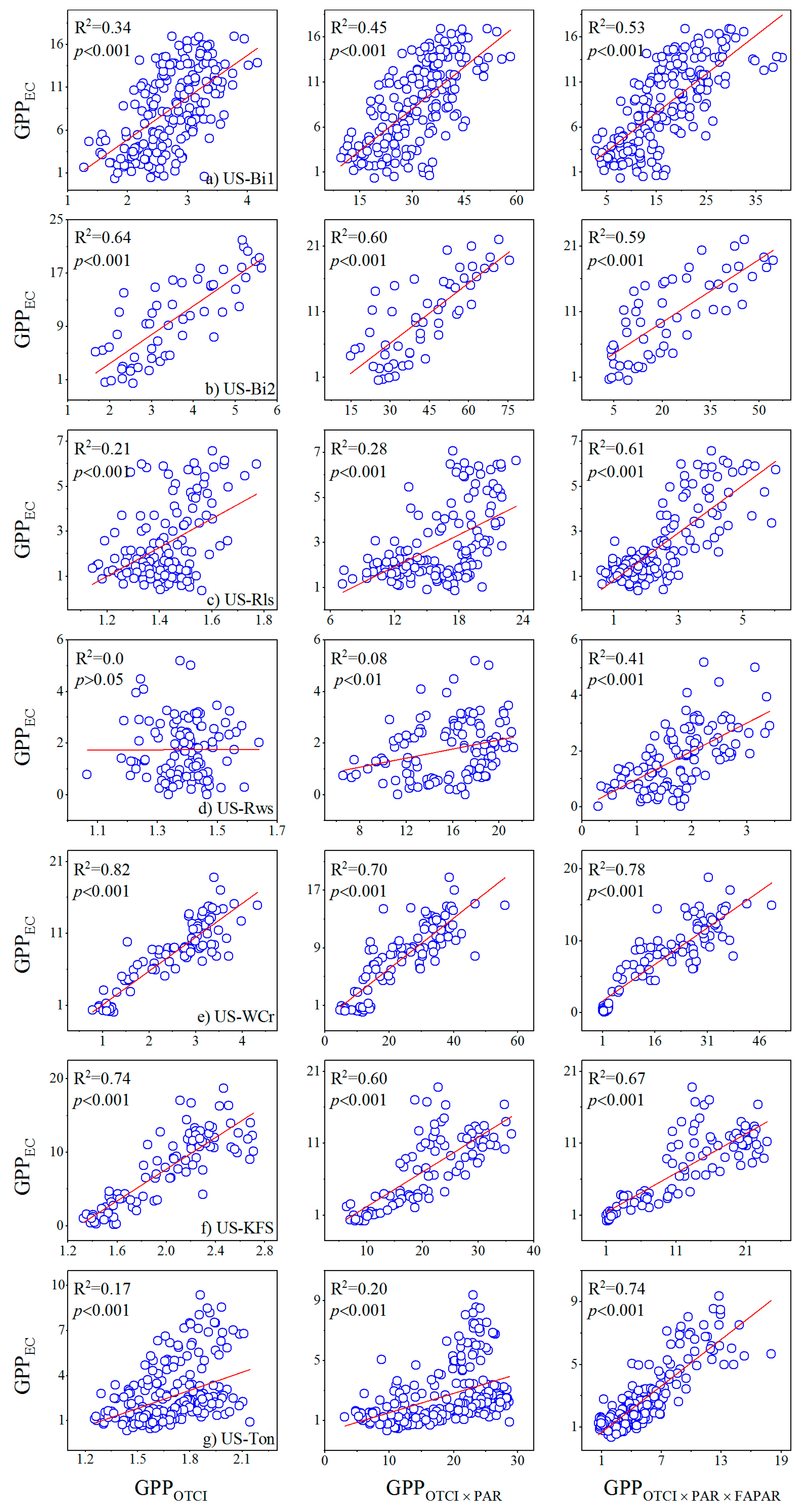
We first compared the performance of GPPOLCI-FAPAR against that of the GPPEC across all sites, including for 2017 and 2018 (Figure 5). Results showed that the US-WCr site obtained the best performance (R2 = 0.76), followed by the US-Ton site with R2 = 0.65, the US-Rls site with R2 = 0.64, and the US-Bi2 site with R2 = 0.55. The R2 values between the GPPOLCI-FAPAR and GPPEC at US-Bi1, US-Rws, and US-KFS were all below 0.5. In terms of the RMSE, the US-Bi2 site produced the maximum error (RMSE = 9.77 g C m−2 d−1), which is nearly twice or more than any other sites (Table 3). This situation was mainly caused by thesubstantial underestimation of GPPOLCI-FAPAR during the peak growth period of corn. This cause of underestimation is also applicable to alfalfa and grass sites. US-Rws had the lowest error with an RMSE of 1.23 g C m−2 d−1 (Table 3). Part of the difference between the US-Rws site and other sites in terms of RMSE was due to the low mean GPP in CSH.
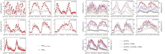
Figure 6 illustrates the temporal variation of GPPOLCI-FAPAR and GPPEC at all sites. Overall, the GPPOLCI-FAPAR effectively matched the GPPEC and generally captured the seasonal variations consistent with the GPPEC at all sites. However, a remarkable difference remains between the GPPEC and GPPOLCI-FAPAR at several sites. Notably, the GPPEC values in most sites were underestimated by the GPPOLCI-FAPAR, except for US-Ton site. As shown in Table 3, the GPPOLCI-FAPAR tracked the GPPEC well at the US-Ton site, with the second lowest bias of 0.64 g C m−2 d−1. Similar to RMSE, the US-Bi2 site had the highest bias (−8.44 g C m−2 d−1). Interestingly, the US-WCr site with a large RMSE also showed the lowest bias. The reason is that part of the bias is offset by the compensation of GPP underestimation in several months in 2017 with overestimation in 2018.
3.3. Agreement between GPPOTCI and GPPEC
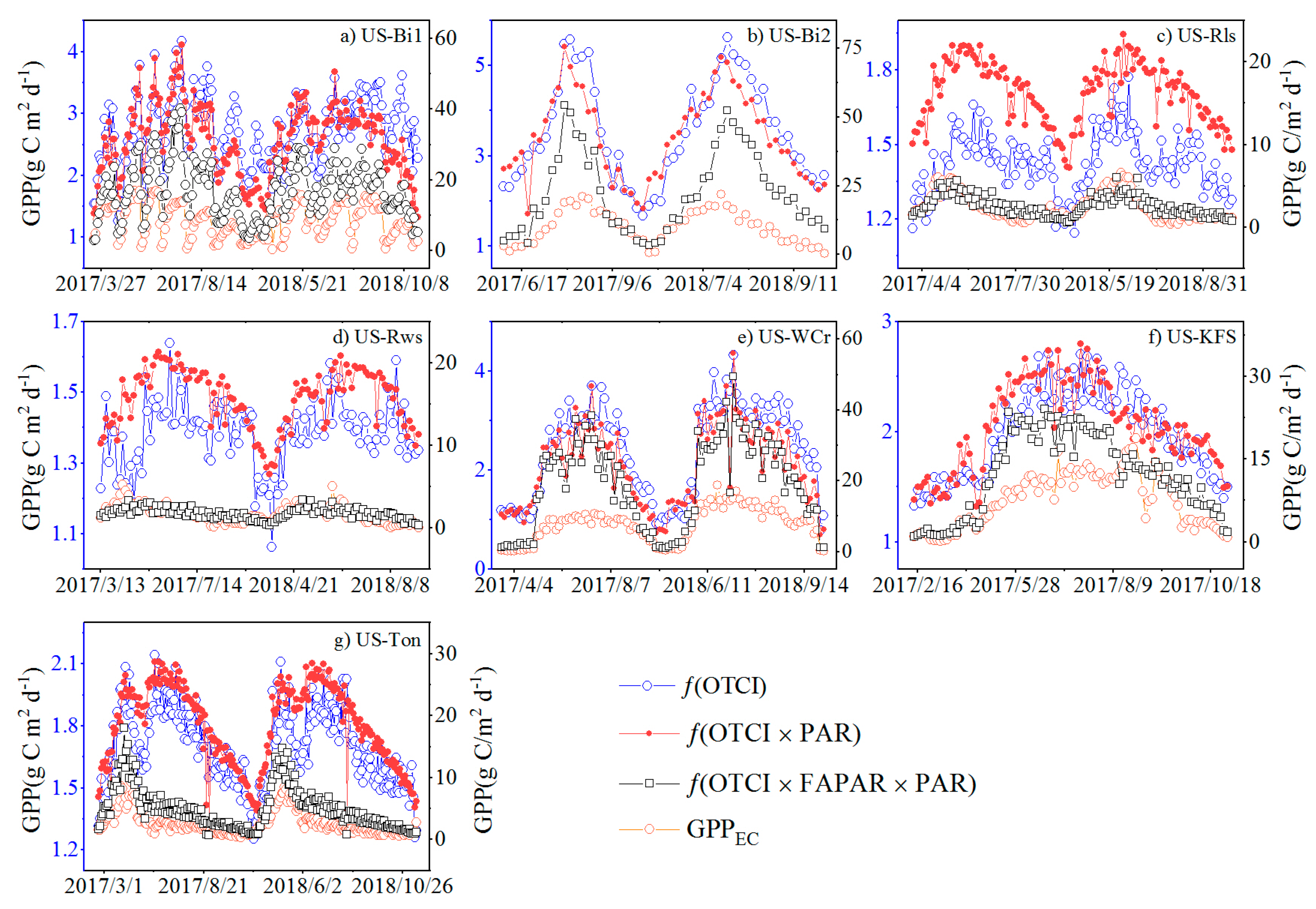
The time series of GPPEC and GPPOTCI that was derived from the three OTCI-driven models in 2017–2018 are presented in Figure 7. Overall, the day-to-day variation in the time series of GPP is evident, whether in GPPEC or GPPOTCI. The consistency in temporal dynamics between GPPEC and GPP from models 1, 2, and 3 were high at most sites. For instance, the growth process of alfalfa from growth to harvest to regrowth was tracked well by the GPP estimated from the OTCI-driven models. However, at the US-Rws site, the GPP obtained from model 3 matched well with the GPPEC while the GPP derived from both models 1 and 2 failed to capture the variation trend. This mismatch can be attributed to the fact that when GPPEC started to decline, the modeled GPP from models 1 and 2 continued to increase. The magnitude of the GPP derived from models 1, 2, and 3 varies considerably across sites. Model 2 gained the maximum value compared with models 1 and 3 among all sites in 2017 and 2018. It is worth noting that the GPP produced by model 3 was close to the GPPEC at the two shrubland sites (US-Rls and US-Rws). At the DBF site, the GPP values modeled at models 2 and 3 were highly consistent, whether in magnitude or in variation trend during the growth period. The reason is that the FAPAR inputted in model 3 is nearly equal to 1, which has a minimal effect on GPP estimation.
The scatter plots between the GPPOTCI based on three OTCI-driven models and the GPPEC for each site are shown in Figure 8. The performance of the three models varies at different sites, thereby demonstrating that the applicability of the three OTCI-driven models is dependent on the biome types. For instance, insignificant correlations of model 1 were obtained at the US-Rws site, whereas the strongest relationship was exhibited with the GPPEC at the US-WCr site. Even for the same type, their performance also differs due to disparate input parameters. For example, model 3 performed much better than model 1 and 2 at the US-Ton, US-Rls and US-Rws sites. Obviously, the inclusion of FAPAR into the model lead to this result. Additionally, strong relationships were established between GPPEC and all the OTCI-driven models at the US-Bi2, US-WCr, and US-KFS sites. At the Bi1 site, a strong to weak relationship was observed from model 3 to model 1. To sum up, model 3, which includes APAR data, provided a significant relationship with GPPEC at all sites, and model 1 is superior to the other two at several sites.
3.4. Comparison between GPPOLCI-FAPAR and GPPMODIS-FAPAR
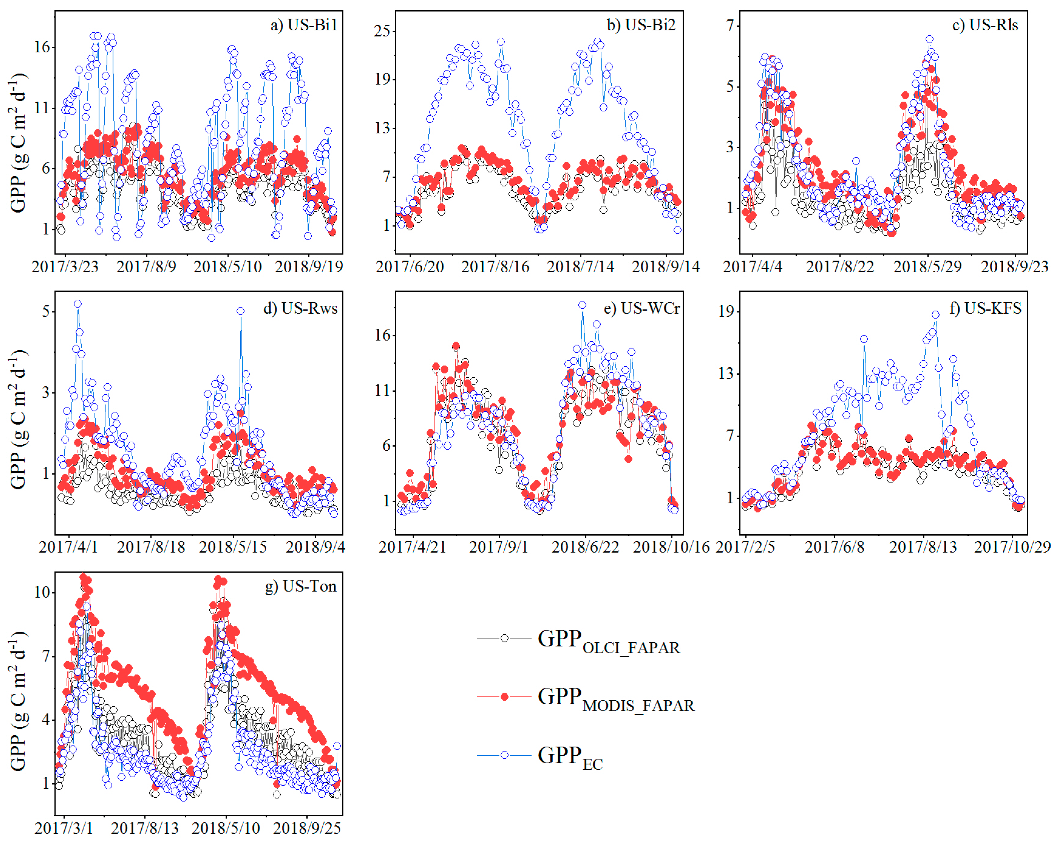
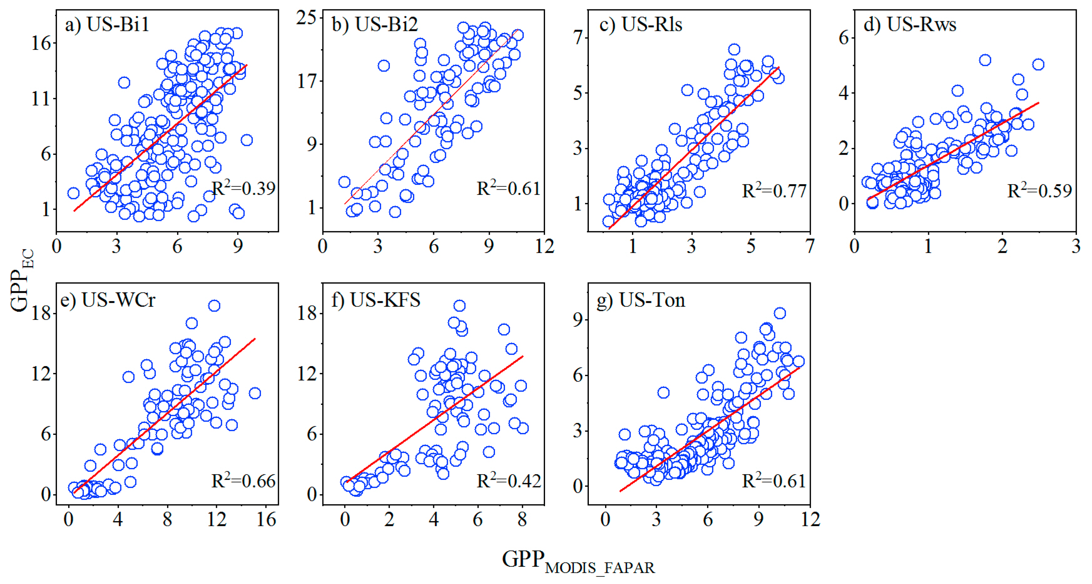
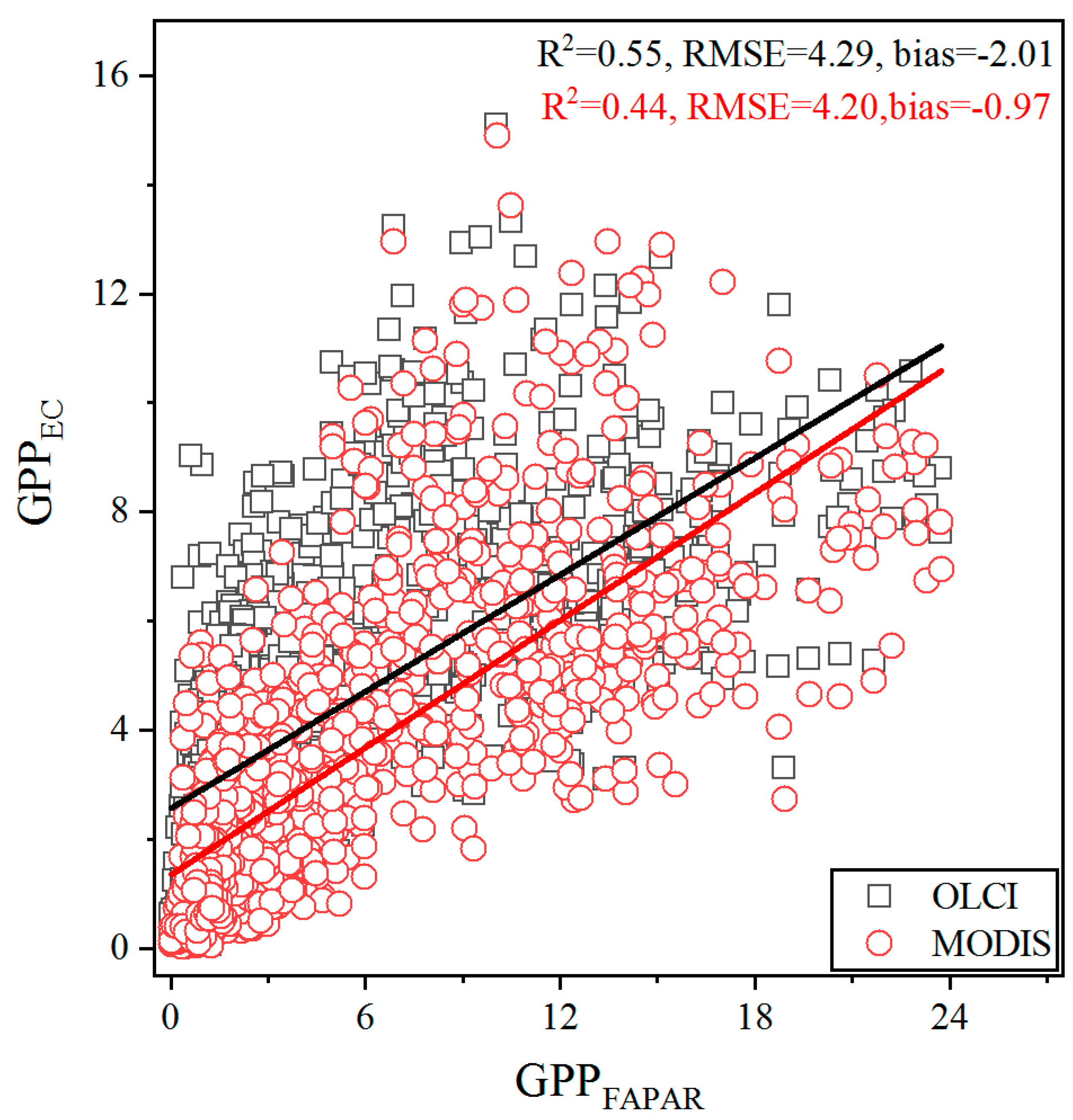
Figure 9 describes the temporal dynamics of GPPEC, GPPMODIS-FAPAR, and GPPOLCI-FAPAR at the seven sites during 2017 and 2018. Obviously, both GPPMODIS-FAPAR and GPPOLCI-FAPAR followed a similar variation trend observed in GPPEC. Nevertheless, GPPMODIS-FAPAR and GPPOLCI-FAPAR, which overestimated or underestimated GPPEC to varying degrees, were also observed at several sites. For example, a substantial underestimation of GPP at two crop sites during peak growth period and a slight overestimation of GPP at the US-Ton site during growing season were clearly identified. As shown in Figure 10, the relationship between GPPMODIS-FAPAR and GPPEC was established. In addition, Table 3 and Table 4 show a comparison of GPPEC, GPPMODIS-FAPAR, and GPPOLCI-FAPAR for each site across two years. As a result, GPPOLCI-FAPAR performed better than GPPMODIS-FAPAR at the US-Bi1, Us-WCr, US-KFS, and US-Ton sites, with a higher R2. With respect to RMSE, the GPPMODIS-FAPAR was superior to GPPOLCI-FAPAR for most sites, except for the Us-WCr and US-Ton sites. In terms of bias, GPPMODIS-FAPAR provided the best performance at most sites, except the US-Ton site. Moreover, the relationship of GPPOLCI-FAPAR and GPPMODIS-FAPAR with GPPEC in the combined sites was established (Figure 11). Overall, the GPPOLCI-FAPAR and GPPMODIS-FAPAR produced acceptable GPP estimates, and if only R2 is considered, the GPPOLCI-FAPAR (R2 = 0.55) performed better than GPPMODIS-FAPAR (R2 = 0.44) across all biomes, demonstrating the applicability of the OLCI FAPAR product for estimating vegetation GPP.
4. Discussion
4.1. Performance Analysis of GPPOLCI-FAPAR Using MODIS GPP Algorithm
The significant relationship between the GPPOLCI-FAPAR and GPPEC across all sites indicates the potential of Sentinel-3 OLCI FAPAR in estimating GPP. However, the performance of the model varies at different sites. The US-WCr site obtained the best performance across all sites. This finding isconsistent with previous studies [5,63]. The reasons can be summarized as follows. Firstly, the seasonal fractional vegetation cover and vegetation structure of DBF were obvious, which can be easily tracked by FAPAR [12]. Secondly, DBF grows in the middle and high latitudes with less cloud cover, and thus time series images with high quality can be obtained [30]. The performance of the US-Ton site was only worse than the US-WCr site. Many studies have reported that the savanna GPP estimation accuracy was lower than other vegetation types due to the misclassification of the savanna [32,64,65]. Unlike savanna, which has a forest canopy cover between 10%–30%, woody savanna’s canopy cover is greater than 30%. Dense vegetation cover can minimize the impact from understory vegetation, which may improve the GPP estimation accuracy. The performance of two shrubland sites was relatively inferior than that of the US-Ton site in our study. Previous studies have indicated that the estimation accuracy of the GPP at shrubland sites varied with regions [36,66]. Temperate regions aregenerally superior than tropical regions. The growth of shrubland is mainly controlled by water ability [32]. As shown in Figure 3c,d, ƒ(VPD) plays a dominant role, especially during shrubland growing season. Moreover, due to the sparse vegetation at the shrubland region, the background soil conditions may have a great impact on GPP estimation [67]. The relationship between GPPOLCI-FAPAR and GPPEC was moderate at the US-Bi1 and US-Bi2 sites. Previous studies have demonstrated that GPP estimation accuracy varied with regions and crop types [68,69,70]. Our study also confirmed this conclusion. It is noteworthy that the RMSE was large at the two cropland sites (Table 3). There are mainly two reasons for this situation. Firstly, the rotation period is different for the two crop types. The US-Bi1 site is a single croppingsystem whereas the US-Bi1 site is a multiple cropping system. However, the threshold of the environmental variables in the MODIS GPP algorithm was set the same for different crop types. Secondly, the algorithm assumed one value of εmax for all C3 and C4 crops, which led to the underestimation of GPP. The GPP estimation accuracy was lowest at the US-KFS site. This was not consistent with other studies, which obtained great performance for grassland [71,72]. The seasonal changes of grassland is obvious and can be tracked well by satellite images [73]. Thus, the flux and climate data uncertainty may lead to the discrepancy between GPPOLCI-FAPAR and GPPEC.
4.2. Performance of OTCI-Driven Models in GPP Estimation
The R2 between GPPOTCI and GPPEC at seven sites showed that at least one of the three OTCI-driven models agreed well with the GPP. The US-Wcr site performed best, whether the model used OTCI only or introduced either PAR or FAPAR. This result was also consistent with that in Section 3.2 using the OLCI FAPAR product. Interestingly, the inclusion ofradiation information (PAR and FAPAR) did much to enhance model performance at the savannas and the two shrubland sites (Figure 4c,d,g). The probable reason is that the impact of soil background on the low vegetation coverage at these sites leads to failure of the OTCI in tracking GPP. By contrast, the addition of PAR and FAPAR appears to have little contribution to the GPP estimation at the US-Bi2, US-WCr, and US-KFS sites (Figure 4b,e,f), as OTCI can directly capture the pronounced seasonal variation of GPP at these sites [17,74].
4.3. Difference between OLCI FAPAR and MODIS FAPAR Product
As described in Section 3.4, the performance of GPPOLCI-FAPAR and GPPMODIS-FAPAR varies at different sites. The main difference between GPPOLCI-FAPAR and GPPMODIS-FAPAR results from the FAPAR product being incorporated in the model. Therefore, the differences between OLCI FAPAR and MODIS FAPAR, which may lead to inconsistency between GPPOLCI-FAPAR and GPPMODIS-FAPAR, are summarized mainly from two aspects. First, the temporal compositing periods of the two products are different. The MODIS FAPAR product is provided in aneight-day interval while the OLCI FAPAR is at a daily interval. For temporal aggregation purposes, MODIS FAPAR is resampled to daily, but its value does not change throughout the eight days.The maximum FAPAR is chosen as the final output value representing the eight days [35]. Second, the MODIS FAPAR and OLCI FAPAR are retrieved from different algorithms. The OLCI FAPAR retrieval algorithm belongs to the family of the JRC (Joint Research Center), which is based on the 1-D RT model, while MODIS FAPAR is derived from the 3-D RT model. The difference between these algorithms is mainly derived from the various definitions and the leaf/wood spectral values assumptions [49].
4.4. Other Sources of Uncertainty, Limitation, and Future Prospects
Additional sources of uncertainty, limitation, and further prospects in simulating GPP are illuminated in the study. First, the quality of the instrument, the randomness of turbulence, the partitioning methods, and gap-filling techniques leading to the random and systematic errors in the flux-derived GPP data is inevitable [75,76]. Second, the mismatches in scale between Sentinel-3 pixels and tower flux footprints lead to further uncertainties. The limitations exist, such as the slow update of the latest EC data and less reliable Sentinel-3 data during the December–April period due to cloudiness contamination. In the future, improvements in the OLCI products through the use of more robust gap-filling methods and in combination with Sentinel-3B data (only Sentinel-3A data wereused in our study to match the flux tower data) may provide even better GPP estimates [28,77].
Although our results showed that GPPOLCI-FAPAR did not always perform better than GPPMODIS-FAPAR, it needs to be emphasized that the objective of our study is not to distinguish which FAPAR product is superior in GPP estimation. Our study demonstrated the potential of OLCI FAPAR and OTCI products for GPP simulation and providedmore complementary solutions to estimate GPP. For example, in terms of data fusion, the OLCI FAPAR product with 10m spatial resolution and nearly daily temporal resolution can be generated by blending Sentinel-2 images and the OLCI FAPAR product using downscaling method and spatiotemporal fusion approaches [45,78]. Then, the same spatial and temporal resolution of the GPP product can be obtained by assimilating FAPAR into LUE models. Moreover, with regard toSIF, the Fluorescence Explorer satellite, which is ESA’s eighth Earth Explorer and is proposed as a tandem with Sentinel-3, is expected to be launched by 2022, and it will provide an integrated package of measurements as well as all the necessary auxiliary information to improve GPP assessment together with Sentinel-3 OLCI and the Sea and Land Surface Temperature Radiometer (SLSTR) [79]. Additionally, this study demonstrated that the MODIS GPP algorithm is also suitable for OLCI FAPAR besides MODIS FAPAR. In years to come, attempts in integrating OLCI FAPAR and the SLSTR land surface temperature (LST) product into other LUE models (e.g., CASA and VPM) to estimate GPP at a large scale are also essential.
5. Conclusions
In this study, we evaluated the performance of two Sentinel-3A OLCI products (i.e., FAPAR and OTCI) in estimating the GPP across seven biomes in 2017–2018. OLCI FAPAR and OTCI products in combination with meteorological data were integrated into the MODIS GPP algorithm and three OTCI-driven models respectively to simulate GPP. GPPOLCI-FAPAR and GPPOTCI were compared with the GPPEC for each site, and a comparison between GPPOLCI-FAPAR and GPPMODIS-FAPAR was established. The main conclusions are summarized as follows:
(1) The relationship between GPPOLCI-FAPAR and GPPEC is significant across all sites. The GPPOLCI-FAPAR correlated best with GPPEC at the US-WCr site (R2 = 0.76) while it performed worst at the US-KFS site (R2 = 0.45).
(2) The inclusion of APAR data in OTCI-driven models exhibited significant relationship with GPPEC for all sites. Nonetheless, the model using only OTCI provided the most varied performance, with the relationship between GPPOTCI and GPPEC from strong to nonsignificant.
(3) The comparison of GPPOLCI-FAPAR and GPPMODIS-FAPAR suggested that they all produced reasonable GPP estimates. In terms of R2, GPPOLCI-FAPAR performed better than the GPPMODIS-FAPAR across all biomes. In the aspect of RMSE and bias, GPPMODIS-FAPAR was superior than GPPOLCI-FAPAR. The main difference between GPPOLCI-FAPAR and GPPMODIS-FAPAR result from the inherent retrieval algorithm and assumptions in the FAPAR product.
In conclusion, the results of this study demonstrate the potential of OLCI FAPAR and OTCI products in GPP estimation, and these results open the possibility of applying them to GPP monitoring at regional and global scales for future studies.
Author Contributions
Conceptualization, Z.Z.; methodology, Z.Z.; software, Z.Z.; validation, Z.Z. and L.Z.; formal analysis, L.Z.; data curation, Z.Z.; writing—original draft preparation, Z.Z.; writing—review and editing, L.Z.; supervision, A.L.; funding acquisition, L.Z. and A.L. All authors have read and agreed to the published version of the manuscript.
Funding
This research was funded by the National Natural Science Foundation of China (41301586) and the Chinese National Funding of Social Sciences (awards 18ZDA040).
Acknowledgments
The authors would like to thank the AmeriFlux community for the eddy covariance data they provided for free, as well as the science teammembers who produce and managethe MODIS and Sentinel-3 data.
Conflicts of Interest
The authors declare no conflict of interest.
References
- Beer, C.; Reichstein, M.; Tomelleri, E.; Ciais, P.; Jung, M.; Carvalhais, N.; Rödenbeck, C.; Arain, M.A.; Baldocchi, D.; Bonan, G.B.; et al. Terrestrial Gross Carbon Dioxide Uptake: Global Distribution and Covariation with Climate. Science 2010, 329, 834–838. [Google Scholar] [CrossRef] [PubMed] [Green Version]
- Zhang, Y.; Xiao, X.; Wu, X.; Zhou, S.; Zhang, G.; Qin, Y.; Dong, J. A global moderate resolution dataset of gross primary production of vegetation for 2000–2016. Sci. Data 2017, 4, 170165. [Google Scholar] [CrossRef] [PubMed] [Green Version]
- Ballantyne, A.; Alden, C.B.; Miller, J.B.; Tans, P.P.; White, J.W.C. Increase in observed net carbon dioxide uptake by land and oceans during the past 50 years. Nature 2012, 488, 70–72. [Google Scholar] [CrossRef] [PubMed]
- Zheng, Y.; Zhang, L.; Xiao, J.; Yuan, W.; Yan, M.; Li, T.; Zhang, Z. Sources of uncertainty in gross primary productivity simulated by light use efficiency models: Model structure, parameters, input data, and spatial resolution. Agric. For. Meteorol. 2018, 263, 242–257. [Google Scholar] [CrossRef]
- Wu, C.; Munger, J.W.; Niu, Z.; Kuang, D. Comparison of multiple models for estimating gross primary production using MODIS and eddy covariance data in Harvard Forest. Remote Sens. Environ. 2010, 114, 2925–2939. [Google Scholar] [CrossRef]
- Osmond, B.; Ananyev, G.; Berry, J.; Langdon, C.; Kolber, Z.S.; Lin, G.; Monson, R.; Nichol, C.; Rascher, U.; Schurr, U.; et al. Changing the way we think about global change research: Scaling up in experimental ecosystem science. Glob. Chang. Biol. 2004, 10, 393–407. [Google Scholar] [CrossRef]
- Schmid, H.P. Source areas for scalars and scalar fluxes. Boundary-Layer Meteorol. 1994, 67, 293–318. [Google Scholar] [CrossRef]
- Xiao, J.; Zhuang, Q.; Baldocchi, D.; Law, B.; Richardson, A.D.; Chen, J.; Oren, R.; Starr, G.; Noormets, A.; Ma, S.; et al. Estimation of net ecosystem carbon exchange for the conterminous United States by combining MODIS and AmeriFlux data. Agric. For. Meteorol. 2008, 148, 1827–1847. [Google Scholar] [CrossRef] [Green Version]
- Behrenfeld, M.J.; Randerson, J.T.; McClain, C.R.; Feldman, G.C.; Los, S.; Tucker, C.J.; Falkowski, P.G.; Field, C.B.; Frouin, R.; Esaias, W.E.; et al. Biospheric Primary Production During an ENSO Transition. Science 2001, 291, 2594–2597. [Google Scholar] [CrossRef] [Green Version]
- Running, S.W.; Thornton, P.E.; Nemani, R.; Glassy, J.M. Global Terrestrial Gross and Net Primary Productivity from the Earth Observing System. Methods Ecosyst. Sci. 2000, 44–57. [Google Scholar]
- Machwitz, M.; Gessner, U.; Conrad, C.; Falk, U.; Richters, J.; Dech, S. Modelling the Gross Primary Productivity of West Africa with the Regional Biomass Model RBM+, using optimized 250 m MODIS FPAR and fractional vegetation cover information. Int. J. Appl. Earth Obs. Geoinf. 2015, 43, 177–194. [Google Scholar] [CrossRef]
- Yuan, W.; Liu, S.; Zhou, G.; Zhou, G.; Tieszen, L.L.; Baldocchi, D.; Bernhofer, C.; Gholz, H.; Goldstein, A.H.; Goulden, M.; et al. Deriving a light use efficiency model from eddy covariance flux data for predicting daily gross primary production across biomes. Agric. For. Meteorol. 2007, 143, 189–207. [Google Scholar] [CrossRef] [Green Version]
- Ryu, Y.; Baldocchi, D.; Kobayashi, H.; van Ingen, C.; Li, J.; Black, T.A.; Beringer, J.; van Gorsel, E.; Knohl, A.; Law, B.; et al. Integration of MODIS land and atmosphere products with a coupled-process model to estimate gross primary productivity and evapotranspiration from 1 km to global scales. Glob. Biogeochem. Cycles 2011, 25. [Google Scholar] [CrossRef] [Green Version]
- Song, C.; Dannenberg, M.P.; Hwang, T. Optical remote sensing of terrestrial ecosystem primary productivity. Prog. Phys. Geogr. Earth Environ. 2013, 37, 834–854. [Google Scholar] [CrossRef]
- Veroustraete, F. On the use of a simple deciduous forest model for the interpretation of climate change effects at the level of carbon dynamics. Ecol. Model. 1994, 75, 221–237. [Google Scholar] [CrossRef]
- Xiao, X.; Zhang, Q.; Braswell, B.; Urbanski, S.; Boles, S.; Wofsy, S.; Moore, B.; Ojima, D. Modeling gross primary production of temperate deciduous broadleaf forest using satellite images and climate data. Remote Sens. Environ. 2004, 91, 256–270. [Google Scholar] [CrossRef]
- Gitelson, A.A.; Viña, A.; Verma, S.; Rundquist, D.; Arkebauer, T.J.; Keydan, G.; Leavitt, B.; Ciganda, V.; Burba, G.; Suyker, A.E. Relationship between gross primary production and chlorophyll content in crops: Implications for the synoptic monitoring of vegetation productivity. J. Geophys. Res. Space Phys. 2006, 111. [Google Scholar] [CrossRef] [Green Version]
- Sims, D.; Rahman, A.; Cordova, V.; El Masri, B.; Baldocchi, D.; Bolstad, P.V.; Flanagan, L.B.; Goldstein, A.H.; Hollinger, D.Y.; Misson, L. A new model of gross primary productivity for North American ecosystems based solely on the enhanced vegetation index and land surface temperature from MODIS. Remote Sens. Environ. 2008, 112, 1633–1646. [Google Scholar] [CrossRef]
- Jung, M.; Reichstein, M.; Margolis, H.A.; Cescatti, A.; Richardson, A.D.; Arain, M.A.; Arneth, A.; Bernhofer, C.; Bonal, D.; Chen, J.; et al. Global patterns of land-atmosphere fluxes of carbon dioxide, latent heat, and sensible heat derived from eddy covariance, satellite, and meteorological observations. J. Geophys. Res. Space Phys. 2011, 116. [Google Scholar] [CrossRef] [Green Version]
- Liu, S.; Zhuang, Q.; He, Y.; Noormets, A.; Chen, J.; Gu, L. Evaluating atmospheric CO2 effects on gross primary productivity and net ecosystem exchanges of terrestrial ecosystems in the conterminous United States using the AmeriFlux data and an artificial neural network approach. Agric. For. Meteorol. 2016, 220, 38–49. [Google Scholar] [CrossRef] [Green Version]
- Sun, Z.; Wang, X.; Zhang, X.; Tani, H.; Guo, E.; Yin, S.; Zhang, T. Evaluating and comparing remote sensing terrestrial GPP models for their response to climate variability and CO2 trends. Sci. Total Environ. 2019, 668, 696–713. [Google Scholar] [CrossRef] [PubMed]
- Monteith, J.L. Solar Radiation and Productivity in Tropical Ecosystems. J. Appl. Ecol. 1972, 9, 747. [Google Scholar] [CrossRef] [Green Version]
- Noumonvi, K.D.; Ferlan, M.; Eler, K.; Alberti, G.; Peressotti, A.; Cerasoli, S. Estimation of Carbon Fluxes from Eddy Covariance Data and Satellite-Derived Vegetation Indices in a Karst Grassland (Podgorski Kras, Slovenia). Remote Sens. 2019, 11, 649. [Google Scholar] [CrossRef] [Green Version]
- Zhang, L.-X.; Zhou, D.-C.; Fan, J.-W.; Hu, Z.-M. Comparison of four light use efficiency models for estimating terrestrial gross primary production. Ecol. Model. 2015, 300, 30–39. [Google Scholar] [CrossRef] [Green Version]
- Prince, S.D.; Goward, S.N. Global Primary Production: A Remote Sensing Approach. J. Biogeogr. 1995, 22, 815. [Google Scholar] [CrossRef]
- Xiao, X.; Hollinger, D.; Aber, J.; Goltz, M.; Davidson, E.A.; Zhang, Q.; Moore, B. Satellite-based modeling of gross primary production in an evergreen needleleaf forest. Remote Sens. Environ. 2004, 89, 519–534. [Google Scholar] [CrossRef]
- Wang, L.; Zhu, H.; Lin, A.; Zou, L.; Qin, W.; Du, Q. Evaluation of the Latest MODIS GPP Products across Multiple Biomes Using Global Eddy Covariance Flux Data. Remote Sens. 2017, 9, 418. [Google Scholar] [CrossRef] [Green Version]
- de Almeida, C.T.; Delgado, R.C.; Galvão, L.S.; Aragão, L.; Ramos, M.C. Improvements of the MODIS Gross Primary Productivity model based on a comprehensive uncertainty assessment over the Brazilian Amazonia. ISPRS J. Photogramm. Remote Sens. 2018, 145, 268–283. [Google Scholar] [CrossRef]
- Zhu, H.; Lin, A.; Wang, L.; Xia, Y.; Zou, L. Evaluation of MODIS Gross Primary Production across Multiple Biomes in China Using Eddy Covariance Flux Data. Remote Sens. 2016, 8, 395. [Google Scholar] [CrossRef] [Green Version]
- Lin, S.; Li, J.; Liu, Q. Overview on estimation accuracy of gross primary productivity with remote sensing methods. J. Remote Sens. 2018, 22, 234–252. [Google Scholar]
- Heinsch, F.; Zhao, M.; Running, S.; Kimball, J.; Nemani, R.; Davis, K.; Bolstad, P.V.; Cook, B.; Desai, A.R.; Ricciuto, D.M.; et al. Evaluation of remote sensing based terrestrial productivity from MODIS using regional tower eddy flux network observations. IEEE Trans. Geosci. Remote Sens. 2006, 44, 1908–1925. [Google Scholar] [CrossRef] [Green Version]
- Sjöström, M.; Zhao, M.; Archibald, S.; Arneth, A.; Cappelaere, B.; Falk, U.; de Grandcourt, A.; Hanan, N.P.; Kergoat, L.; Kutsch, W.; et al. Evaluation of MODIS gross primary productivity for Africa using eddy covariance data. Remote Sens. Environ. 2013, 131, 275–286. [Google Scholar] [CrossRef]
- Cheng, Y.-B.; Zhang, Q.; Lyapustin, A.; Wang, Y.; Middleton, E.M. Impacts of light use efficiency and fPAR parameterization on gross primary production modeling. Agric. For. Meteorol. 2014, 189, 187–197. [Google Scholar] [CrossRef]
- He, M.; Ju, W.; Zhou, Y.; Chen, J.; He, H.; Wang, S.; Wang, H.; Guan, D.; Yan, J.; Li, Y.; et al. Development of a two-leaf light use efficiency model for improving the calculation of terrestrial gross primary productivity. Agric. For. Meteorol. 2013, 173, 28–39. [Google Scholar] [CrossRef]
- Running, S.W.; Glassy, J.M.; Thornton, P.E. MODIS Daily Photosynthesis (PSN) and Annual Net Primary Production (NPP) Product (MOD17) Algorithm Theoretical Basis Document; University of Montana: Missoula, Montana, 1999. [Google Scholar]
- Yuan, W.; Cai, W.; Xia, J.; Chen, J.; Liu, S.; Dong, W.; Merbold, L.; Law, B.; Arain, A.; Beringer, J.; et al. Global comparison of light use efficiency models for simulating terrestrial vegetation gross primary production based on the LaThuile database. Agric. For. Meteorol. 2014, 192, 108–120. [Google Scholar] [CrossRef]
- Wu, C.; Niu, Z.; Gao, S. Gross primary production estimation from MODIS data with vegetation index and photosynthetically active radiation in maize. J. Geophys. Res. Space Phys. 2010, 115. [Google Scholar] [CrossRef] [Green Version]
- Nestola, E.; Calfapietra, C.; Emmerton, C.A.; Wong, C.Y.S.; Thayer, D.R.; Gamon, J.A. Monitoring Grassland Seasonal Carbon Dynamics, by Integrating MODIS NDVI, Proximal Optical Sampling, and Eddy Covariance Measurements. Remote Sens. 2016, 8, 260. [Google Scholar] [CrossRef] [Green Version]
- Lin, S.; Li, J.; Liu, Q.; Li, L.; Zhao, J.; Yu, W. Evaluating the Effectiveness of Using Vegetation Indices Based on Red-Edge Reflectance from Sentinel-2 to Estimate Gross Primary Productivity. Remote Sens. 2019, 11, 1303. [Google Scholar] [CrossRef] [Green Version]
- Cerasoli, S.; Campagnolo, M.; Faria, J.; Nogueira, C.; Caldeira, M. On estimating the gross primary productivity of Mediterranean grasslands under different fertilization regimes using vegetation indices and hyperspectral reflectance. Biogeosciences 2018, 15, 5455–5471. [Google Scholar] [CrossRef] [Green Version]
- Dash, J.; Curran, P.J. The MERIS terrestrial chlorophyll index. Int. J. Remote Sens. 2004, 25, 5403–5413. [Google Scholar] [CrossRef]
- Loozen, Y.; Rebel, K.T.; Karssenberg, D.; Wassen, M.J.; Sardans, J.; Peñuelas, J.; de Jong, S.M. Remote sensing of canopy nitrogen at regional scale in Mediterranean forests using the spaceborne MERIS Terrestrial Chlorophyll Index. Biogeosciences 2018, 15, 2723–2742. [Google Scholar] [CrossRef] [Green Version]
- Rossini, M.; Cogliati, S.; Meroni, M.; Migliavacca, M.; Galvagno, M.; Busetto, L.; Cremonese, E.; Julitta, T.; Siniscalco, C.; Di Cella, U.M.; et al. Remote sensing-based estimation of gross primary production in a subalpine grassland. Biogeosciences 2012, 9, 2565–2584. [Google Scholar] [CrossRef] [Green Version]
- Harris, A.; Dash, J. The potential of the MERIS Terrestrial Chlorophyll Index for carbon flux estimation. Remote Sens. Environ. 2010, 114, 1856–1862. [Google Scholar] [CrossRef] [Green Version]
- Wang, Q.; Atkinson, P.M. Spatio-temporal fusion for daily Sentinel-2 images. Remote Sens. Environ. 2018, 204, 31–42. [Google Scholar] [CrossRef] [Green Version]
- Wang, X.; Ling, F.; Yao, H.; Liu, Y.; Xu, S. Unsupervised Sub-Pixel Water Body Mapping with Sentinel-3 OLCI Image. Remote Sens. 2019, 11, 327. [Google Scholar] [CrossRef] [Green Version]
- Donlon, C.; Berruti, B.; Buongiorno, A.; Ferreira, M.-H.; Féménias, P.; Frerick, J.; Goryl, P.; Klein, U.; Laur, H.; Mavrocordatos, C.; et al. The Global Monitoring for Environment and Security (GMES) Sentinel-3 mission. Remote Sens. Environ. 2012, 120, 37–57. [Google Scholar] [CrossRef]
- Jin, J.; Jiang, H.; Zhang, X.; Wang, Y. Characterizing Spatial-Temporal Variations in Vegetation Phenology over the North-South Transect of Northeast Asia Based upon the MERIS Terrestrial Chlorophyll Index. Terr. Atmos. Ocean. Sci. 2012, 23, 413. [Google Scholar] [CrossRef] [Green Version]
- Zhang, Z.; Zhang, Y.; Zhang, Y.; Gobron, N.; Frankenberg, C.; Wang, S.; Li, Z. The potential of satellite FPAR product for GPP estimation: An indirect evaluation using solar-induced chlorophyll fluorescence. Remote Sens. Environ. 2020, 240, 111686. [Google Scholar] [CrossRef]
- Hemes, K.S.; Chamberlain, S.D.; Eichelmann, E.; Anthony, T.; Valach, A.; Kasak, K.; Szutu, D.; Verfaillie, J.; Silver, W.L.; Baldocchi, D. Assessing the carbon and climate benefit of restoring degraded agricultural peat soils to managed wetlands. Agric. For. Meteorol. 2019, 268, 202–214. [Google Scholar] [CrossRef]
- Renwick, K.M.; Fellows, A.; Flerchinger, G.N.; Lohse, K.A.; Clark, P.E.; Smith, W.K.; Emmett, K.; Poulter, B. Modeling phenological controls on carbon dynamics in dryland sagebrush ecosystems. Agric. For. Meteorol. 2019, 274, 85–94. [Google Scholar] [CrossRef]
- Zhang, Q.; Ficklin, D.L.; Manzoni, S.; Wang, L.; Way, D.; Phillips, R.P.; A Novick, K. Response of ecosystem intrinsic water use efficiency and gross primary productivity to rising vapor pressure deficit. Environ. Res. Lett. 2019, 14, 074023. [Google Scholar] [CrossRef]
- Brunsell, N.; Nippert, J.B.; Buck, T.L. Impacts of seasonality and surface heterogeneity on water-use efficiency in mesic grasslands. Ecohydrology 2013, 7, 1223–1233. [Google Scholar] [CrossRef]
- Boden, T.A.; Krassovski, M.; Yang, B. The AmeriFlux data activity and data system: An evolving collection of data management techniques, tools, products, and services. Geosci. Instrum. Methods Data Syst. 2013, 2, 165–176. [Google Scholar] [CrossRef] [Green Version]
- Piao, S.; Fang, J.; Zhou, L.; Zhu, B.; Tan, K.; Tao, S. Changes in vegetation net primary productivity from 1982 to 1999 in China. Glob. Biogeochem. Cycles 2005, 19. [Google Scholar] [CrossRef] [Green Version]
- Gorbon, N. Uncertainties Assessment for MERIS/OLCI fAPAR; European Commission: Brussels, Belgium, 2015. [Google Scholar]
- Knyazikhin, Y.; Glassy, J.; Privette, J.L.; Tian, Y.; Running, S.W. MODIS Leaf Area Index (LAI) and Fraction of Photosynthetically Active Radiation Absorbed by Vegetation (FPAR) Product (MOD15) Algorithm Theoretical Basis Document; Boston University: Boston, MA, USA, 1999. [Google Scholar]
- Myneni, R.B.; Hoffman, S.; Knyazikhin, Y.; Privette, J.L.; Glassy, J.; Tian, Y.; Wang, Y.; Song, X.; Zhang, Y.; Smith, G.R.; et al. Global products of vegetation leaf area and fraction absorbed PAR from year one of MODIS data. Remote Sens. Environ. 2002, 83, 214–231. [Google Scholar] [CrossRef] [Green Version]
- Xiao, X. Light absorption by leaf chlorophyll and maximum light use efficiency. IEEE Trans. Geosci. Remote Sens. 2006, 44, 1933–1935. [Google Scholar] [CrossRef]
- Boyd, D.S.; Almond, S.; Dash, J.; Curran, P.J.; Hill, R.A.; Foody, G.M. Evaluation of Envisat MERIS Terrestrial Chlorophyll Index-Based Models for the Estimation of Terrestrial Gross Primary Productivity. IEEE Geosci. Remote Sens. Lett. 2011, 9, 457–461. [Google Scholar] [CrossRef]
- Yoder, B.J.; Waring, R.H. The normalized difference vegetation index of small Douglas-fir canopies with varying chlorophyll concentrations. Remote Sens. Environ. 1994, 49, 81–91. [Google Scholar] [CrossRef]
- Richardson, A.D.; Hollinger, D.Y. A method to estimate the additional uncertainty in gap-filled NEE resulting from long gaps in the CO2 flux record. Agric. For. Meteorol. 2007, 147, 199–208. [Google Scholar] [CrossRef]
- Verma, M.; Friedl, M.; Law, B.; Bonal, D.; Kiely, G.; Black, T.; Wohlfahrt, G.; Moors, E.; Montagnani, L.; Marcolla, B.; et al. Improving the performance of remote sensing models for capturing intra- and inter-annual variations in daily GPP: An analysis using global FLUXNET tower data. Agric. For. Meteorol. 2015, 214, 416–429. [Google Scholar] [CrossRef] [Green Version]
- Jin, C.; Xiao, X.; Merbold, L.; Arneth, A.; Veenendaal, E.; Kutsch, W.L. Phenology and gross primary production of two dominant savanna woodland ecosystems in Southern Africa. Remote Sens. Environ. 2013, 135, 189–201. [Google Scholar] [CrossRef]
- Kanniah, K.D.; Beringer, J.; Hutley, L.B.; Tapper, N.J.; Zhu, X. Evaluation of Collections 4 and 5 of the MODIS Gross Primary Productivity product and algorithm improvement at a tropical savanna site in northern Australia. Remote Sens. Environ. 2009, 113, 1808–1822. [Google Scholar] [CrossRef]
- Jiang, C.; Ryu, Y. Multi-scale evaluation of global gross primary productivity and evapotranspiration products derived from Breathing Earth System Simulator (BESS). Remote Sens. Environ. 2016, 186, 528–547. [Google Scholar] [CrossRef]
- Zhang, L.; Zhou, D.; Fan, J.; Guo, Q.; Chen, S.; Wang, R.; Li, Y. Contrasting the Performance of Eight Satellite-Based GPP Models in Water-Limited and Temperature-Limited Grassland Ecosystems. Remote Sens. 2019, 11, 1333. [Google Scholar] [CrossRef] [Green Version]
- Kalfas, J.L.; Xiao, X.; Vanegas, D.X.; Verma, S.B.; Suyker, A.E. Modeling gross primary production of irrigated and rain-fed maize using MODIS imagery and CO2 flux tower data. Agric. For. Meteorol. 2011, 151, 1514–1528. [Google Scholar] [CrossRef] [Green Version]
- Yuan, W.; Cai, W.; Nguy-Robertson, A.L.; Fang, H.; Suyker, A.; Chen, Y.; Dong, W.; Liu, S.; Zhang, H. Uncertainty in simulating gross primary production of cropland ecosystem from satellite-based models. Agric. For. Meteorol. 2015, 207, 48–57. [Google Scholar] [CrossRef] [Green Version]
- Yan, H.; Fu, Y.; Xiao, X.; Huang, H.Q.; He, H.; Ediger, L. Modeling gross primary productivity for winter wheat–maize double cropping system using MODIS time series and CO2 eddy flux tower data. Agric. Ecosyst. Environ. 2009, 129, 391–400. [Google Scholar] [CrossRef]
- Liu, Z.; Wang, L.; Wang, S. Comparison of Different GPP Models in China Using MODIS Image and ChinaFLUX Data. Remote Sens. 2014, 6, 10215–10231. [Google Scholar] [CrossRef] [Green Version]
- Zhang, F.; Chen, J.M.; Chen, J.; Gough, C.M.; Martin, T.A.; Dragoni, D. Evaluating spatial and temporal patterns of MODIS GPP over the conterminous U.S. against flux measurements and a process model. Remote Sens. Environ. 2012, 124, 717–729. [Google Scholar] [CrossRef]
- Li, Z.; Yu, G.-R.; Xiao, X.; Li, Y.; Zhao, X.; Ren, C.; Zhang, L.; Fu, Y. Modeling gross primary production of alpine ecosystems in the Tibetan Plateau using MODIS images and climate data. Remote Sens. Environ. 2007, 107, 510–519. [Google Scholar] [CrossRef]
- Wu, C.; Niu, Z.; Tang, Q.; Huang, W.; Rivard, B.; Feng, J. Remote estimation of gross primary production in wheat using chlorophyll-related vegetation indices. Agric. For. Meteorol. 2009, 149, 1015–1021. [Google Scholar] [CrossRef]
- Richardson, A.D.; Hollinger, D.Y.; Burba, G.; Davis, K.J.; Flanagan, L.B.; Katul, G.G.; Munger, J.W.; Ricciuto, D.M.; Stoy, P.C.; Suyker, A.E.; et al. A multi-site analysis of random error in tower-based measurements of carbon and energy fluxes. Agric. For. Meteorol. 2006, 136, 1–18. [Google Scholar] [CrossRef] [Green Version]
- Lucas-Moffat, A.; Papale, D.; Reichstein, M.; Hollinger, D.Y.; Richardson, A.D.; Barr, A.; Beckstein, C.; Braswell, B.; Churkina, G.; Desai, A.R.; et al. Comprehensive comparison of gap-filling techniques for eddy covariance net carbon fluxes. Agric. For. Meteorol. 2007, 147, 209–232. [Google Scholar] [CrossRef]
- Liu, Z.; Wu, C.; Peng, D.; Wang, S.; Gonsamo, A.; Fang, B.; Yuan, W. Improved modeling of gross primary production from a better representation of photosynthetic components in vegetation canopy. Agric. For. Meteorol. 2017, 233, 222–234. [Google Scholar] [CrossRef]
- Yu, T.; Sun, R.; Xiao, Z.; Zhang, Q.; Wang, J.; Liu, G. Generation of High-Resolution Vegetation Productivity from a Downscaling Method. Remote Sens. 2018, 10, 1748. [Google Scholar] [CrossRef] [Green Version]
- Tenjo, C.; Rivera-Caicedo, J.P.; Sabater, N.; Servera, J.V.; Alonso, L.; Verrelst, J.; Moreno, J. Design of a Generic 3-D Scene Generator for Passive Optical Missions and Its Implementation for the ESA’s FLEX/Sentinel-3 Tandem Mission. IEEE Trans. Geosci. Remote Sens. 2018, 56, 1290–1307. [Google Scholar] [CrossRef]
Figure 1.
Geographical location of AmeriFlux sites in this study.

Figure 2.
Temporal dynamics of the daily flux tower gross primary productivity (GPPEC) at seven eddy flux tower sites in 2017 and 2018. Colored shadings denote the uncertainties. (a): alfalfa site, (b): corn site, (c): closed shrubland site, (d): open shrubland site, (e): deciduous broadleaf forest site, (f): grass site, (g): woody savanna site.

Figure 3.
Temporal dynamics of the minimum temperature (Tmin) and vapor pressure deficit (VPD) for all seven sites in 2017 and 2018. (a–g) represent the sites the same as Figure 2.
Figure 3.
Temporal dynamics of the minimum temperature (Tmin) and vapor pressure deficit (VPD) for all seven sites in 2017 and 2018. (a–g) represent the sites the same as Figure 2.

Figure 4.
Temporal dynamics ofscalar factors (ƒ(Tmin) and ƒ(VPD)) in the left column; fraction of absorbed photosynthetically active radiation (FAPAR), photosynthetically active radiation (PAR), and GPPEC in the right column for all seven sites in 2017 and 2018. (a–g) represent the sites the same as Figure 2.

Figure 5.
Scatterplots between GPPEC and GPPOLCI-FAPAR (GPP for the Ocean and Land Colour Instrument FAPAR product) for all sites in 2017 and 2018. Significance levels: p < 0.001. (a–g) represent the sites the same as Figure 2.
Figure 5.
Scatterplots between GPPEC and GPPOLCI-FAPAR (GPP for the Ocean and Land Colour Instrument FAPAR product) for all sites in 2017 and 2018. Significance levels: p < 0.001. (a–g) represent the sites the same as Figure 2.

Figure 6.
Temporal dynamics of GPPEC and GPPOLCI-FAPAR for all sites in 2017 and 2018.

Figure 7.
Temporal dynamics of GPPEC and three OTCI-driven GPPOTCI for all sites in 2017 and 2018.

Figure 8.
Scatterplots between GPPEC and GPPOTCI for all sites in 2017 and 2018. The left column represents model 1: GPP = ƒ(OTCI), the middle column represents model 2: GPP = ƒ(OTCI × PAR), and the right column represents model 3: GPP = ƒ (OTCI × PAR × FAPAR). (a–g) represent the sites the same as Figure 2.

Figure 9.
Temporal dynamics of GPPMODIS-FAPAR (GPP with the FAPARfrom the Moderate Resolution Imaging Spectroradiometer (MODIS)), GPPOLCI-FAPAR, and GPPEC for all sites in 2017 and 2018. (a–g) represent the sites the same as Figure 2.
Figure 9.
Temporal dynamics of GPPMODIS-FAPAR (GPP with the FAPARfrom the Moderate Resolution Imaging Spectroradiometer (MODIS)), GPPOLCI-FAPAR, and GPPEC for all sites in 2017 and 2018. (a–g) represent the sites the same as Figure 2.

Figure 10.
Scatterplots between GPPEC and GPPMODIS-FAPAR for all sites in 2017 and 2018. Significance levels: p < 0.001. (a–g) represent the sites the same as Figure 2.
Figure 10.
Scatterplots between GPPEC and GPPMODIS-FAPAR for all sites in 2017 and 2018. Significance levels: p < 0.001. (a–g) represent the sites the same as Figure 2.

Figure 11.
Scatterplots betweenthe flux tower GPP and the GPP estimated from satellite FAPAR products for all combined data across all sites. Black and red lines represent the GPP derived from the OLCI and MODIS FAPAR respectively. Significance levels: p < 0.001.
Figure 11.
Scatterplots betweenthe flux tower GPP and the GPP estimated from satellite FAPAR products for all combined data across all sites. Black and red lines represent the GPP derived from the OLCI and MODIS FAPAR respectively. Significance levels: p < 0.001.


Table 1.
List of AmeriFlux eddy covariance tower sites used in this study.
| Site ID | Site Name | Latitude | Longitude | IGBP | Main Species | Measurement Height/Canopy Height (m) | MAT | MAP | MAT and MAP Period | Years Used | Reference |
|---|---|---|---|---|---|---|---|---|---|---|---|
| US-Bi1 | Bouldin Island Alfalfa | 38.1 | −121.5 | CRO | Alfalfa (Medicago sativa L.) | 3.9/0.5 | 16 | 338 | 2016–2018 | 2017–2018 | [50] |
| US-Bi2 | Bouldin Island corn | 38.11 | −121.54 | CRO | Corn (Zea mays) | 5.1/2.6 | 16 | 338 | 2017–2018 | 2017–2018 | [50] |
| US-Rls | RCEW Low Sagebrush | 43.14 | −116.74 | CSH | Low sagebrush | * | 8.4 | 333 | 2014–2018 | 2017–2018 | [51] |
| US-Rws | Reynolds Creek Wyoming big sagebrush | 43.17 | −116.71 | OSH | Wyoming big sagebrush | * | 8.9 | 290 | 2014–2018 | 2017–2018 | [51] |
| US-WCr | Willow Creek | 45.81 | −90.08 | DBF | Sugar maple, Acer saccharum | 30/25 | 4.02 | 787 | 1999–2018 | 2017–2018 | [52] |
| US-KFS | Kansas Field Station | 39.06 | −95.19 | GRA | Bromus inermis | */0.5 | 12 | 1014 | 2007–2017 | 2017 | [53] |
| US-Ton | Tonzi Ranch | 38.43 | −120.97 | WSA | Blue oak | 23/13 | 15.8 | 559 | 2001–2018 | 2017–2018 | [52] |
MAT: mean annual temperature (°C); MAP: mean annual long-term precipitation (mm); IGBP: International Geosphere-Biosphere Programme; CRO: croplands; CSH: close shrublands; OSH: open shrubland; DBF: deciduous broadleaf forests; GRA: grasslands; WSA: woody savanna; * denotes no data.
Table 2.
Biome properties lookup table for the MODIS GPP algorithm.
| Biome Types | DBF | CSH | OSH | WSA | GRA | CRO |
|---|---|---|---|---|---|---|
| εmax (g C m−2 d−1) | 1.165 | 1.281 | 0.841 | 1.239 | 0.860 | 1.044 |
| TMINmin (°C) | −6.00 | −8.00 | −8.00 | −8.00 | −8.00 | −8.00 |
| TMINmax (°C) | 9.94 | 8.61 | 8.80 | 11.39 | 12.02 | 12.02 |
| VPDmin (Pa) | 650.0 | 650.0 | 650.0 | 650.0 | 650.0 | 650.0 |
| VPDmax (Pa) | 2300.0 | 4700.0 | 4800.0 | 3200.0 | 5300.0 | 4300.0 |
Table 3.
Coefficient of determination (R2), root mean square error (RMSE, g C m−2 d−1) and bias (g C m−2 d−1) between GPPOLCI-FAPAR and GPPEC for seven sites.
Table 3.
Coefficient of determination (R2), root mean square error (RMSE, g C m−2 d−1) and bias (g C m−2 d−1) between GPPOLCI-FAPAR and GPPEC for seven sites.
| Site ID | R2 | RMSE | Bias |
|---|---|---|---|
| US-Bi1 | 0.45 | 5.18 | −3.6 |
| Us-Bi2 | 0.55 | 9.77 | −8.13 |
| US-Rls | 0.64 | 1.36 | −0.88 |
| US-Rws | 0.5 | 1.23 | −0.89 |
| US-WCr | 0.76 | 2.42 | −0.61 |
| US-KFS | 0.45 | 5.54 | −4.03 |
| US-Ton | 0.65 | 1.39 | 0.64 |
Note: Highest R2, lowest RMSE, and lowest bias value are shown in bold. Significance levels: p < 0.001.
Table 4.
Coefficient of determination (R2), root mean square error (RMSE, g C m−2 d−1), and bias (g C m−2 d−1) between GPPMODIS-FAPAR and GPPEC for seven sites.
Table 4.
Coefficient of determination (R2), root mean square error (RMSE, g C m−2 d−1), and bias (g C m−2 d−1) between GPPMODIS-FAPAR and GPPEC for seven sites.
| Site ID | R2 | RMSE | Bias |
|---|---|---|---|
| US-Bi1 | 0.39 | 4.61 | −2.6 |
| Us-Bi2 | 0.61 | 9.14 | −7.41 |
| US-Rls | 0.77 | 0.79 | 0.05 |
| US-Rws | 0.59 | 0.87 | −0.45 |
| US-WCr | 0.66 | 2.81 | −0.1 |
| US-KFS | 0.42 | 5.26 | −3.57 |
| US-Ton | 0.42 | 3.11 | 2.74 |
Note: Highest R2, lowest RMSE, and lowest bias value are shown in bold. Significance levels: p < 0.001.
© 2020 by the authors. Licensee MDPI, Basel, Switzerland. This article is an open access article distributed under the terms and conditions of the Creative Commons Attribution (CC BY) license (http://creativecommons.org/licenses/by/4.0/).
Share and Cite
MDPI and ACS Style
Zhang, Z.; Zhao, L.; Lin, A. Evaluating the Performance of Sentinel-3A OLCI Land Products for Gross Primary Productivity Estimation Using AmeriFlux Data. Remote Sens. 2020, 12, 1927. https://0-doi-org.brum.beds.ac.uk/10.3390/rs12121927
AMA Style
Zhang Z, Zhao L, Lin A. Evaluating the Performance of Sentinel-3A OLCI Land Products for Gross Primary Productivity Estimation Using AmeriFlux Data. Remote Sensing. 2020; 12(12):1927. https://0-doi-org.brum.beds.ac.uk/10.3390/rs12121927
Chicago/Turabian StyleZhang, Zhijiang, Lin Zhao, and Aiwen Lin. 2020. "Evaluating the Performance of Sentinel-3A OLCI Land Products for Gross Primary Productivity Estimation Using AmeriFlux Data" Remote Sensing 12, no. 12: 1927. https://0-doi-org.brum.beds.ac.uk/10.3390/rs12121927
Note that from the first issue of 2016, this journal uses article numbers instead of page numbers. See further details here.