Monitoring the Seasonal Hydrology of Alpine Wetlands in Response to Snow Cover Dynamics and Summer Climate: A Novel Approach with Sentinel-2

Abstract

Climate change in the European Alps during recent years has led to decreased snow cover duration as well as increases in the frequency and intensity of summer heat waves. The risk of drought for alpine wetlands and temporary pools, which rely on water from snowmelt and provide habitat for specialist plant and amphibian biodiversity, is largely unknown and understudied in this context. Here, we test and validate a novel application of Sentinel-2 imagery aimed at quantifying seasonal variation in water surface area in the context of 95 small (median surface area <100 m²) and shallow (median depth of 20 cm) alpine wetlands in the French Alps, using a linear spectral unmixing approach. For three study years (2016–2018), we used path-analysis to correlate mid-summer water surface area to annual metrics of snowpack (depth and duration) and spring and summer climate (temperature and precipitation). We further sought to evaluate potential biotic responses to drought for study years by monitoring the survival of common frog (Rana temporaria) tadpoles and wetland plant biomass production quantified using peak Normalized Difference Vegetation Index (NDVI). We found strong agreement between citizen science-based observations of water surface area and Sentinel-2 based estimates (R² = 0.8–0.9). Mid-summer watershed snow cover duration and summer temperatures emerged as the most important factors regulating alpine wetland hydrology, while the effects of summer precipitation, and local and watershed snow melt-out timing were not significant. We found that a lack of summer snowfields in 2017 combined with a summer heat wave resulted in a significant decrease in mid-summer water surface area, and led to the drying up of certain wetlands as well as the observed mortality of tadpoles. We did not observe a negative effect of the 2017 summer on the biomass production of wetland vegetation, suggesting that wetlands that maintain soil moisture may act as favorable microhabitats for above treeline vegetation during dry years. Our work introduces a remote sensing-based protocol for monitoring the surface hydrology of alpine wetland habitats at the regional scale. Given that climate models predict continued reduction of snow cover in the Alps during the coming years, as well as particularly intense warming during the summer months, our conclusions underscore the vulnerability of alpine wetlands in the face of ongoing climate change.

1. Introduction

Recent climate warming in the European Alps is currently reshaping alpine landscapes and ecosystems. Increases in mean temperature in the Alps are amplified with respect to the global average [1] and warming has accelerated markedly since the 1980s [2]. Rising mean temperatures have been accompanied by an increase in the frequency and intensity of extreme events, such as summer heat waves, during the last twenty years [3]. Shifts in air temperature have led to significant reductions in glacier mass and extent [4,5], as well as a 4–5 week reduction in snow cover duration since the 1970s in the Swiss Alps [6]. Mountain plant species are moving upslope and increasing biomass production in response to climate warming [7,8,9], and vegetation belts within the Alps are expected to continue to shift upward in response to 21st century climate change [10].

Alpine wetlands are situated at the confluence of the aforementioned recent changes in climate, cryosphere, hydrology, and vegetation. Located between the treeline and snowfields and glaciers, alpine semipermanent pools and ponds (hereafter referred to more generally as wetlands) are present throughout most of world’s mountains and are defined as small (1 m² to a few square hectares) and shallow water bodies characterized by at least the seasonal presence of surface water [11]. The hydrology of alpine wetlands is understood to be tightly linked to watershed runoff from rain and snowmelt [11]. Predicted decreases in snow cover duration combined with continued glacier retreat are expected to diminish summer water runoff, particularly during the second half of the 21st century [12], which could decrease available surface water for alpine wetlands. In the Swiss Alps, recent warming has been associated with increases in the abundance of generalist thermophilous plant species at the expense of specialized wetland species [13]. Amphibian populations are known to be declining at the global scale due to climate change, disease, and habitat degradation [14,15], and amphibian habitat loss has been documented in mountainous regions throughout Australia, North America, and Central America [16]. Notably, the drying up of wetland pools in Australia has been linked to the local mortality of an endangered Australian frog species, Pseudophyrne pengilleyi [17]. In light of these examples, studies linking climate, wetland hydrology, and biodiversity responses in the Alps remain lacking. Improving our knowledge of the ecohydrological functioning of alpine wetlands is of particular importance in order to inform wetland biodiversity conservation measures and also from the standpoint of ecosystem services, given that wetland habitats are known to provide important downstream regulatory services such as aquifer recharge, flood mitigation, and denitrification [18].

Recent improvements in widely available optical satellite imagery are enabling unprecedented opportunities for tracking the responses of mountain ecosystems to climate variability and change. Specifically, the Sentinel-2 satellite mission, launched in 2015, includes an unprecedented combination of 5 day temporal revisit, 10 m spatial resolution, ten spectral bands ranging from visible to short-wave infrared, and a free and open access data policy. In mountainous regions, Sentinel-2 has already been utilized for a number of applications, including for example generating high-resolution snow cover maps across the Alps and Pyrenees [19], quantifying the effects of snow cover duration on alpine plant community habitat [20], and improving land cover maps of dwarf Ericaceae shrubs above treeline [21]. We propose that the relatively high spatial, temporal, and spectral resolution of Sentinel-2 could be utilized to enhance monitoring of the seasonal hydrology of alpine wetlands.

In this study, we focus on alpine pools and ponds characterized by seasonal snow cover and fluctuating amounts of surface water over the course of the summer season. In contrast to alpine lakes, biological communities in small alpine water bodies are strongly driven by water availability and hydroperiod [11,22]. In this context, binary classification approaches based on spectral indices [23], or object-oriented classification that have previously been used to map large wetlands and water bodies [24], may be insufficient to map small (e.g., <100 m²) and constantly fluctuating mountain pools. Furthermore, high spatial resolution images with pixel size below 25 m², obtained, for example, using aerial photographs, specialized satellite platforms such as PLEIADES or SPOT 6/7, or drone imagery, tend to have highly limited temporal and spectral resolution and can require expensive and time consuming acquisition and preprocessing protocols [25].

To respond to these methodological challenges, we propose using linear spectral unmixing, which was originally developed as a method for mapping desert shrublands using Landsat imagery [26]. This approach allows for mapping sub-pixel fractions that correspond to objects that are smaller than the spatial resolution of available imagery, which, in this case, means smaller than a 100 m² Sentinel-2 pixel. Based on the assumption that the reflectance values of image pixels are the result of varying mixtures of components, or endmembers, this technique has been used for numerous applications in plant cover mapping and forestry (see, e.g., in [27,28]), soil and erosion mapping (see, e.g., in [29]) and more recently for snow algae detection in Antarctica [30]. We propose multi-temporal spectral unmixing as a potential approach for quantifying the surface dynamics of wetlands, in terms of snow cover and surface water.

In this paper, we test the use of linear spectral unmixing as a means of quantifying seasonal variation in the water surface area of small alpine wetlands located in the northern French Alps with respect to field observations of water surface area. We further utilize available Sentinel-2 imagery to quantify snow cover duration at the watershed and local wetland scales. For three study years (2016 to 2018), we correlate interannual variability in meteorological and snow cover parameters to mid-summer water surface area, in order to identify the most important parameters linked to drought risk. Finally, we assess the potential of our method for quantifying biotic responses of wetland communities to drought, by monitoring the development and survival of common frog (Rana temporaria) tadpoles in select sites and by quantifying wetland vegetation biomass production.

2. Materials and Methods

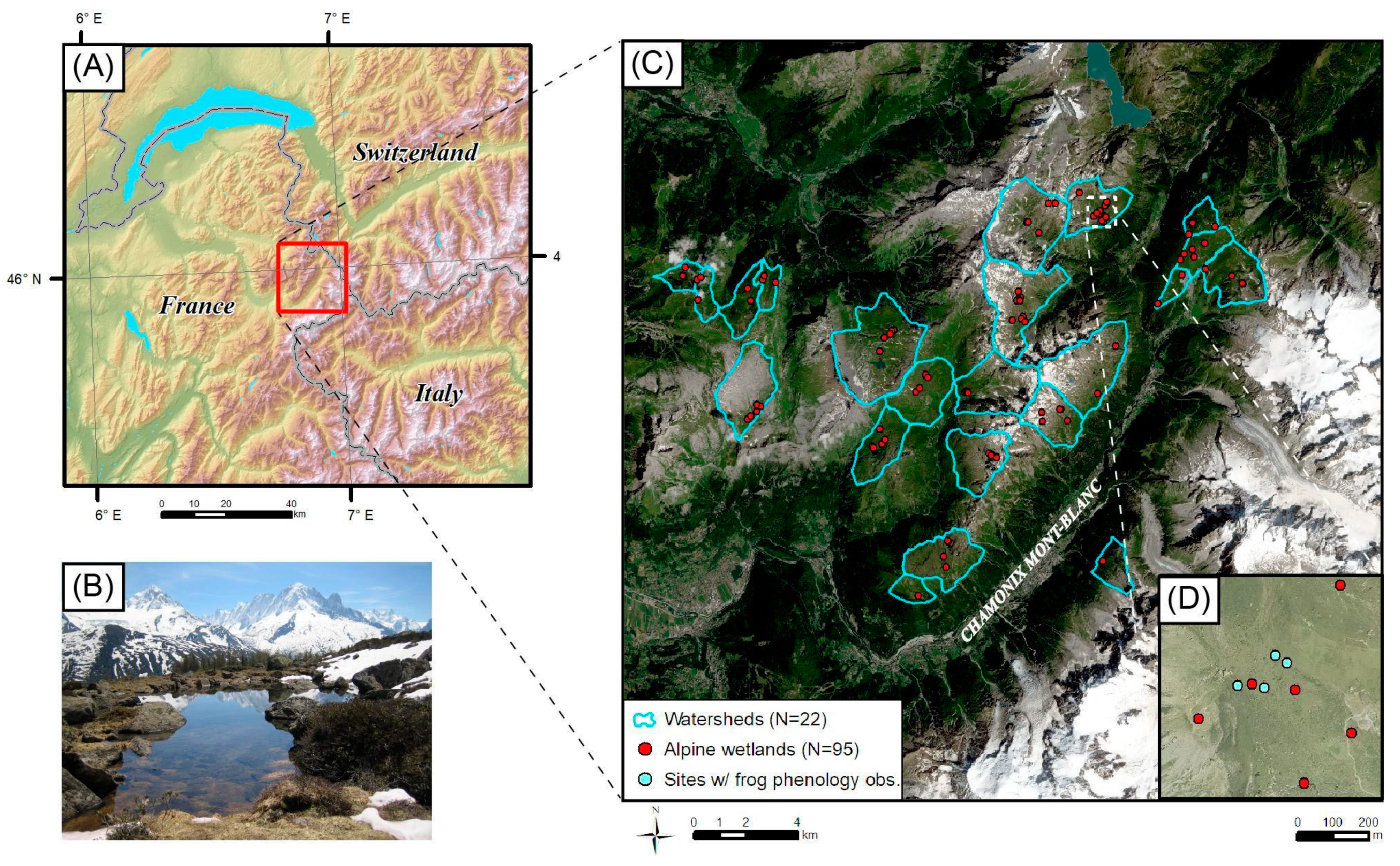
2.1. Study Area and Fieldwork

This work was carried out in the Chamonix valley in the Mont-Blanc massif and located in the northern French Alps (Figure 1). Studied sites (N = 95) were identified over the course of two field seasons carried out between mid-July and mid-August: 20 wetlands were identified in 2010, while an additional 75 wetlands were visited during the summers of 2017 and 2018. We focused on ponds and pools located in open areas without forest cover above 1800 m a.s.l., and that contained surface water at the time of the field survey (lakes, rivers, streams, peat bogs, and wetlands characterized by damp soil were excluded from the analysis). Observed water surface area of target wetlands varied from 3 to 5000 m² with a mean of 511 m², with water depth ranging from 3 cm to 3 m with a mean depth of 44 cm. The elevation of studied wetlands ranged from 1820 to 2600 m a.s.l., with a mean elevation of 2100 m a.s.l.. Sites were distributed across 22 alpine watersheds (Figure 1C). Bedrock varied from limestone in the western portion of the study area, to schist and limestone for central and northeastern wetlands and granite in the case of the southeastern most watershed. Many of the watersheds are characterized by persistent snowfields during the summer months (Figure 1C).

During the summers of 2016, 2017, and 2018 we carried out weekly visits to four wetlands at the Loriaz site (Figure 1D) to monitor the development of common frog (Rana temporaria) tadpoles. During each visit, we recorded the presence of frog eggs as well as the number of egg clusters, followed by the phenological stage attained by the tadpoles (see Figure S1). We also noted local mortality of the tadpole population, in the case of drought.

2.2. Sentinel-2 Imagery

For this analysis, we relied on multi-spectral images acquired by the Sentinel-2 satellites (2A and 2B), which jointly provide a 5 day revisit time since March 2017. Available spectral bands range from visible to shortwave infrared, with 4 bands at 10 m spatial resolution (B2: 490 nm, B3: 560 nm, B4: 665 nm, B8: 842 nm) and 6 bands at 20 m spatial resolution (B5: 705 nm, B6: 740 nm, B7: 783 nm, B8a: 865 nm, B11: 1610 nm, B12: 2190 nm). We downloaded 76 Sentinel-2A and B (hereafter referred to as Sentinel-2) scenes for the T32TLS tile and for the years 2016, 2017, and 2018 from the French THEIA platform.

Acquired images were preprocessed by the THEIA to level 2A (i.e., orthorectified product in surface reflectance). Images were corrected for both atmospheric and topographic effects [31,32], which are particularly important in mountainous areas where slope angle and aspect affects pixel illumination [33]. Level-2A products were provided with cloud and shadow masks, which we applied to all spectral bands. In total, we analyzed 23 dates in 2016, 25 dates in 2017, and 28 dates in 2018 between the months of February and November of each year.

2.3. Endmember Selection and Spectral Unmixing

Spectral endmembers were identified using a 50 cm resolution aerial photograph acquired in 2009 covering the study area. We hypothesized that all alpine wetland pixels could be composed of a mixture of the following endmembers, water, vegetation, rock and bareground, and snow. Given that all sites were located above the treeline with low-stature vegetation, we considered it unnecessary to include shadow as a spectral endmember. Using the aerial photographs for reference, we identified between three and four visually pure Sentinel-2 pixels for each target endmember class, representing an area of homogenous cover for at least a 50 × 50 m zone in order to avoid edge effects. We then extracted spectral values for identified endmember pixels from a Sentinel-2A image acquired on August 3, 2016. We averaged spectral values for each endmember class and carried out a principal component analysis (PCA) using the ade4 package in R.

Linear spectral unmixing allows for the estimation of sub-pixel fractions of target endmembers and is suitable for mapping phenomena that vary at finer scales than the spatial resolution of available imagery [26]. By resolving an ordinary least squares equation, the algorithm estimates the fractional cover of endmembers resulting in observed spectral values [34]. In Equation (1), ρ_j represents the observed spectral band values (in this case from the Sentinel-2 reflectance value for a given band and pixel), F_i represents endmember fractions that are equivalent to slope values in the linear model, ρ_{j, i} represents the known reflectance values of target endmembers, and E_j represents an error term estimated for each band. The sum of estimated fractions (∑ F_i) is constrained to be equal to 1 (Equation (2)). In this configuration, F_i is the only unknown value and can be solved for using the following equations:

$${\mathsf{\rho }}_j={\displaystyle \sum }_{i=1}^m{F}_{i }\times {\mathsf{\rho }}_j+E_j$$

(1)

$${\displaystyle \sum }_{i=1}^m{F}_i=1$$

(2)

where j corresponds to the number spectral bands, i corresponds to a given endmember, and m represents the the number of endmembers.

For each acquired Sentinel-2 scene, we resampled 20 m bands to 10 m using bilinear interpolation, and created a stack covering the study area. We extracted Sentinel-2 spectral values for the GPS coordinates of each wetland using two approaches: (i) a simple method extracting spectral values for the pixel overlapping the coordinates, and (ii) using a 20 m buffer to extract spectral values in the vicinity of the target wetland. The resulting tables were defined as spectral libraries, with each column representing one of the ten Sentinel-2 bands and each row representing a target pixel. We then used the “unmix” function in the hsdar R package to estimate the fractional cover of endmembers for each pixel and for each date. Error values and fraction estimates resulting from the simple extract were stored directly for each wetland. For results of the 20 m buffer, we summed the surface area of each endmember across all pixels and stored values for each Sentinel-2 scene date. In order to quantify water levels during the critical midsummer period when drought is most likely, we calculated the mean water surface area for available dates between July 15 and August 15 (Water surface area; Figure S2).

2.4. Field Validation

In order to validate Sentinel-2 based estimates of water surface area, we carried out field observations with different volunteer groups for four summer dates between 2016 and 2019. Volunteers included local elementary school students accompanied by teachers, local adults, visiting university students, and tourists. Group size ranged from 6 to 15 participants, which were split into at least two groups. In the field, groups were asked to delimit a 30 × 30 m grid centered on the target wetland and GPS coordinate, composed of nine smaller 10 m sub-squares (see Figure S3). For each 10 × 10 m square, volunteers conducted visual estimates of the percent cover of different endmembers (rock and bareground, vegetation, water, and snow). For each plot, two separate groups observed the central grid cell in order to quantify observer error. Based on values for the nine grid cells, we calculated mean and total water surface area for each site as noted by volunteers.

For target wetlands, we extracted water surface area estimates for the nine nearest Sentinel-2 pixels centered on the wetland GPS coordinate. Field visits were coordinated so as to occur either the same day or within 1 day of the passage of one of the Sentinel-2 satellites. We calculated mean and total water surface area from Sentinel-2 fractional estimates for the nine pixels overlapping the target water body, and correlated these values with field observations. Given that both field and satellite observations were subject to errors, we utilized standardized major axis regression in the smatr R-package to assess agreement between Sentinel-2 and ground-based observations.

2.5. Mapping Snow Cover and Wetland Plant Biomass

For each Sentinel-2 scene, we calculated the Normalized Difference Snow Index (NDSI) and the Normalized Difference Vegetation Index (NDVI) and the using Equations (3) and (4):

$$NDSI=\frac{\left(Rgreen-Rswir\right)}{(Rgreen+Rswir)}$$

(3)

$$NDVI=\frac{\left(Rnir-Rred\right)}{\left(Rnir+Rred\right)}$$

(4)

where NIR is the reflectance in the near-infrared band (Band 8), red corresponds reflectance in Band 4, green corresponds to Band 3, and SWIR is shortwave infrared (Band 11). We applied a 0.4 threshold to NDSI values to estimate the presence or absence of snow cover for 10 m pixels for each Sentinel-2 scene [35]. For each date, we also calculated the percentage of watersheds covered by snow. We also estimated local snow melt out date for wetlands based on the following criteria, NDSI < 0.4 and a snow fraction estimate of 0. Finally, for each year and each wetland, we extracted the maximum value of NDVI between July 15 and August 15 as a proxy of peak biomass and plant photosynthetic activity.

2.6. Meteorological Data and Structural Equation Modeling

We obtained daily meteorological and snowpack data for the last thirty years for 300 m elevation bands within the Mont-Blanc massif from the Safran-CROCUS atmosphere-snowpack reanalysis, provided by Météo-France and the Centre d’Etudes de la Neige [36,37]. Data were downloaded from the open access Aeris portal [38]. Based on our hypotheses, we extracted the following monthly parameters for each year (1988 to 2018): mean snowpack height for the month of March (March snowpack depth), sum of growing degree days (>0 °C) for 2 m air temperature in March and April (March–April GDD), sum of growing degree days (>0 °C) for June and July (June–July GDD), and the sum of rainfall in June and July (June–July precip.). For study years (2016–2018), we assigned values from the 300 m elevation class corresponding to each study site. In order to contextualize study years within the last thirty years and for the 1950 to 2250 m a.s.l. elevation band, we calculated average values and annual anomalies for all variables over the 1988 to 2018 period.

We derived the following spatial snow cover variables from Sentinel-2 imagery: the date that watershed snow cover fell below 30%, based on NDSI-based binary snow cover maps (Watershed snowmelt), the date of local snow melt-out for wetlands (defined by fractional snow cover below 10% for wetland pixels, Wetland snowmelt) and the average percent snow cover of watersheds between July 15 and August 15 based on NDSI snow cover maps (Summer snowfields).

We utilized a structural equation modeling (SEM) approach to test linear relationships between meteorological and snowpack parameters and observed midsummer water surface area. As an extension of path analysis, SEM represents an appropriate statistical framework for modeling multivariate and hierarchical effects of predictors on target response variables [39,40]. We first standardized values using the “decostand” function in the vegan R package, and subsequently verified that pairwise relationships between variables could be modeled using ordinary least squares linear regressions. We then tested multiple model pathways, based on the following hypotheses; in all models, we expected midsummer Water surface area to be correlated with June-July GDD, June–July precip., and with snowpack. In order to identify which snowpack parameter was the most significant, we tested models using Watershed snowmelt, Wetland snowmelt, and Summer snowfields as predictors. We also systematically tested models with and without summer precipitation as a predictor of Water surface area. To test the effects of snowpack depth on spatial snow cover parameters, we correlated each snowpack parameter with March snowpack depth and an air temperature variable (April–May GDD for Wetland and Watershed snowmelt, and June–July GDD in the case of Summer snowfields). We compared models using the following criteria: goodness-of-fit requiring a χ² chi-square p-value greater than 0.05 [41], the Akaike Information Criterion (AIC) value, and explained variance (R²) of Water surface area.

3. Results

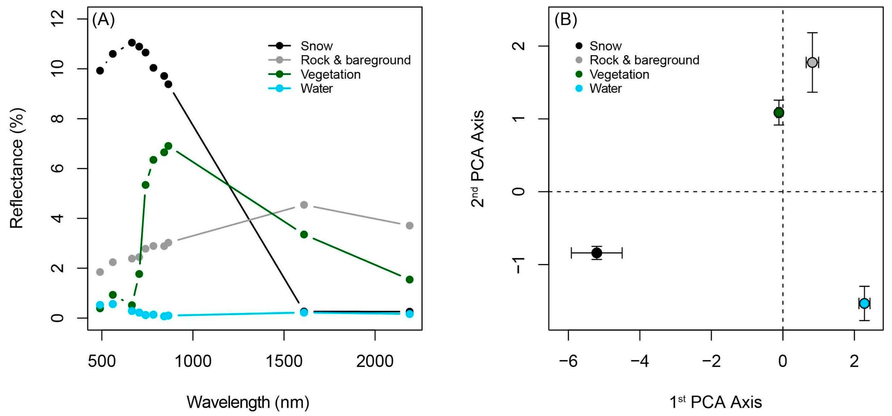
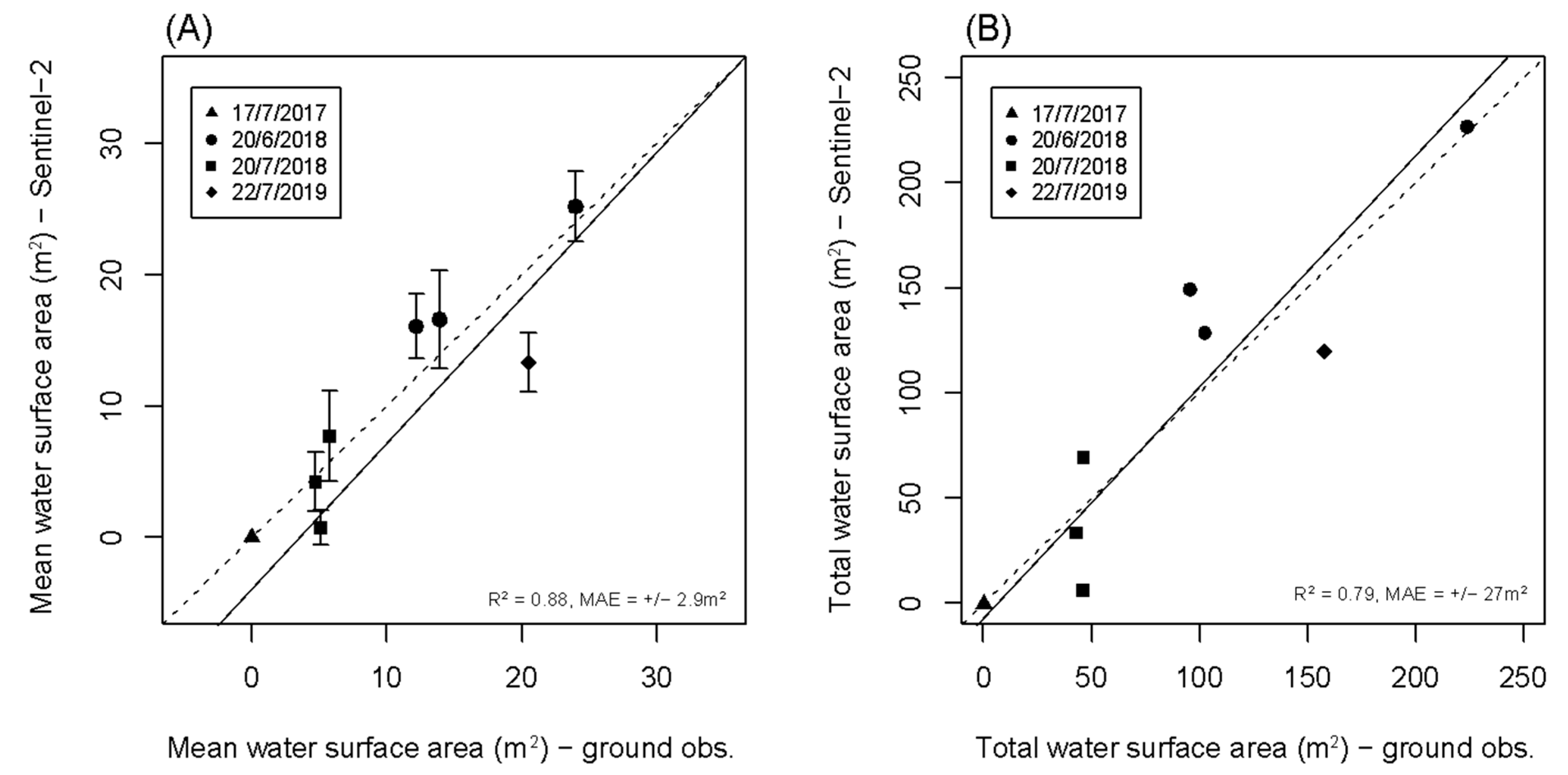
3.1. Spectral Endmember Differentiation and Method Validation

Selected endmembers exhibited distinct spectral signals with respect to Sentinel-2 bands, both in terms of mean reflectance values (Figure 2A) and multivariate PCA coordinates (Figure 2B). Vegetation and bareground were the most closely related spectral endmembers, while snow and water exhibited highly distinctive spectral signatures. Error resulting from spectral unmixing was low (around 0.01%) across scene dates, with slightly higher errors at the beginning (June) and end (September) of the summer season, potentially due to persistent snow cover and the variable state of plant canopies during the fall season compared to the early-August reference used for endmember definition (Figure S2).

Wetlands underwent a characteristic transition from full snow cover during the winter months to a mixture of water, bareground, and vegetation between snowmelt-out in the spring and snow onset in the fall (Figure 3). Water surface area varied over the course of the summer season, which was corroborated by field observations and visually confirmed using drone imagery (Figure 3). Although localized drought was apparent immediately surrounding a target wetland in July 2017 (Figure 3A), the utilization of the 20 m buffer enabled the detection of water within a broader vicinity adjacent to the target wetland (Figure 3).

We observed strong agreement between field observations of water surface area and estimates derived from Sentinel-2 images (Figure 4). We found positive linear relationships with respect to mean water surface area (Figure 4A, R² = 0.88) and total water surface area (Figure 4B, R² = 0.79) for target wetland areas. Some systematic error was apparent in the case of mean water surface area, and Sentinel-2 tended to slightly underestimate water surface area for low quantities of water (<10 m²) with respect to field observations (Figure 4A). Although the linear relationship was not as strong compared to mean water surface area, in the case of total water surface area, the relationship exhibited no systematic error and the linear trend closely followed the 1:1 reference line (Figure 4B). We observed a mean absolute error (MAE) of ±27 m² for total water surface area over a 900 m² area, which corresponded to a 3% error rate. Different volunteer groups demonstrated strong agreement between visual estimates of endmember ground cover, including for water (R² = 0.76), vegetation (R² = 0.76), and rock and bare ground (R² = 0.80; Figure S4).

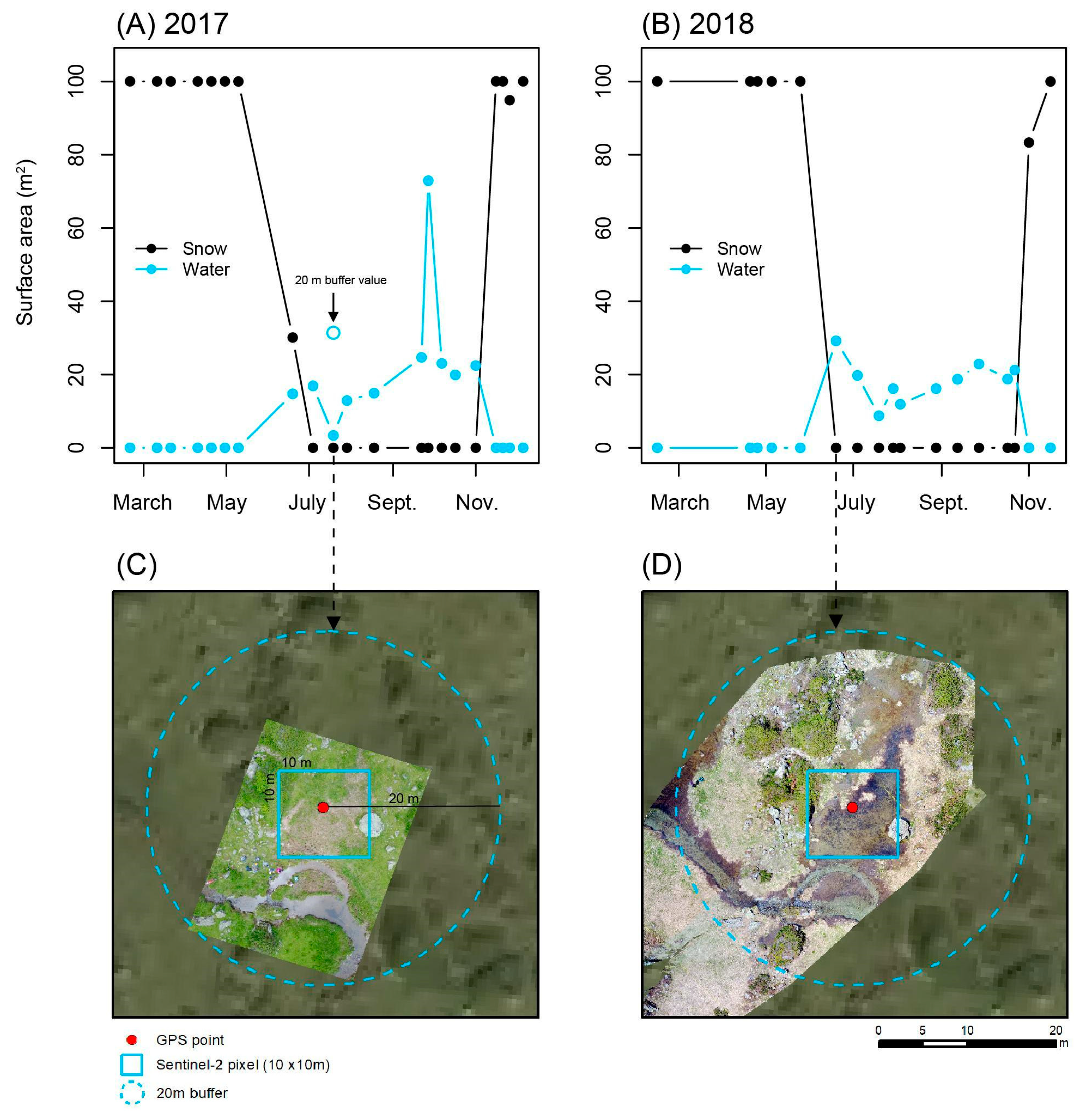
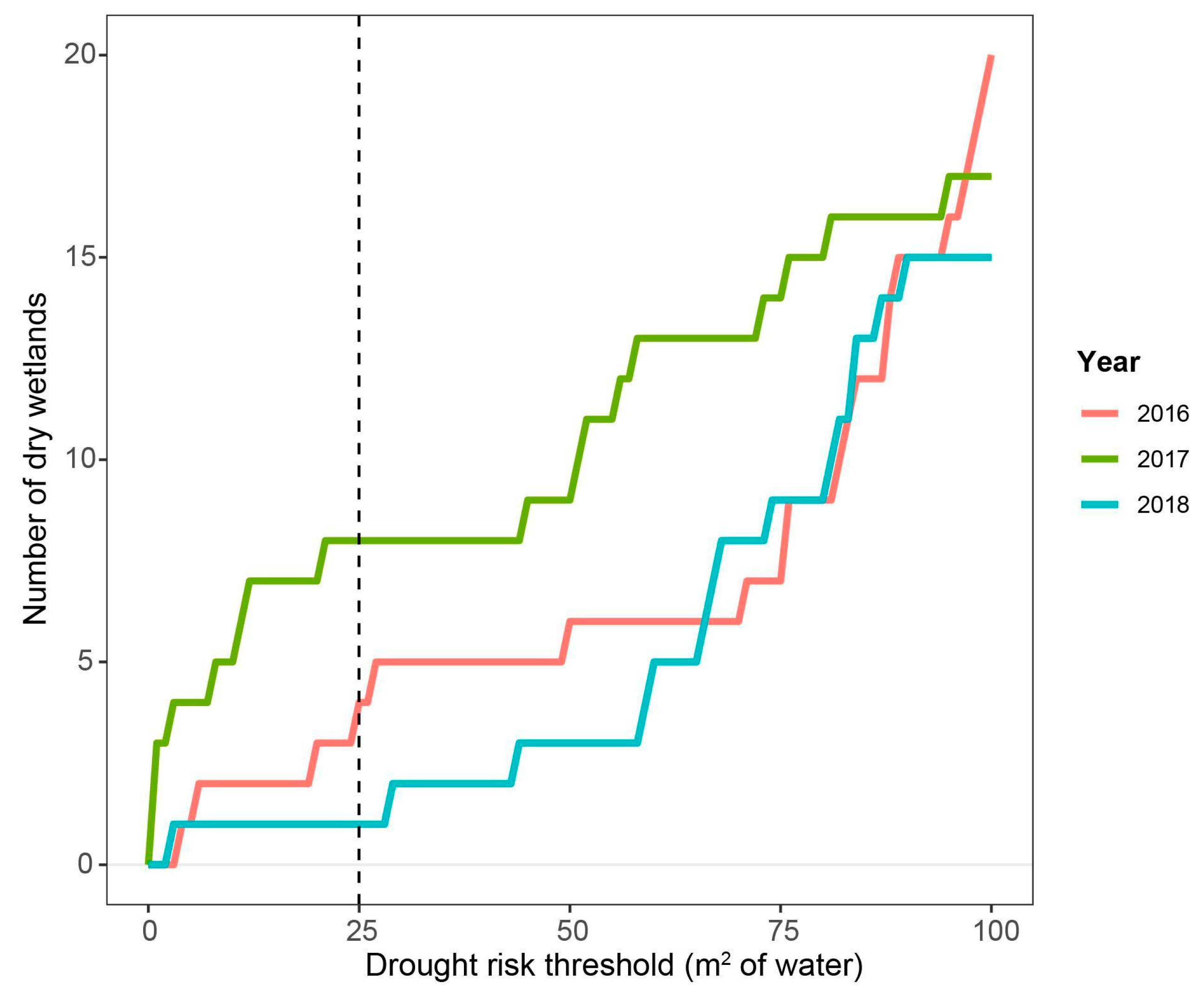
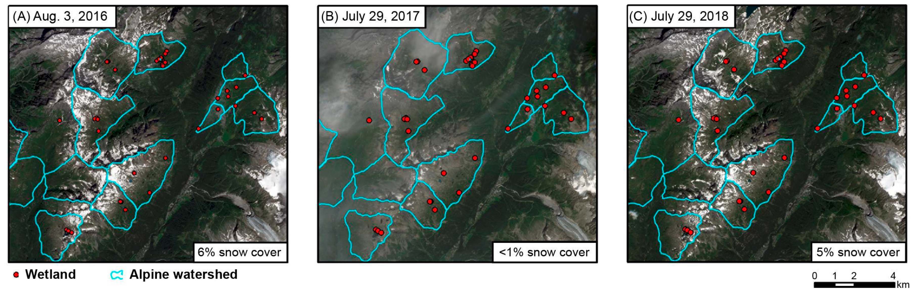
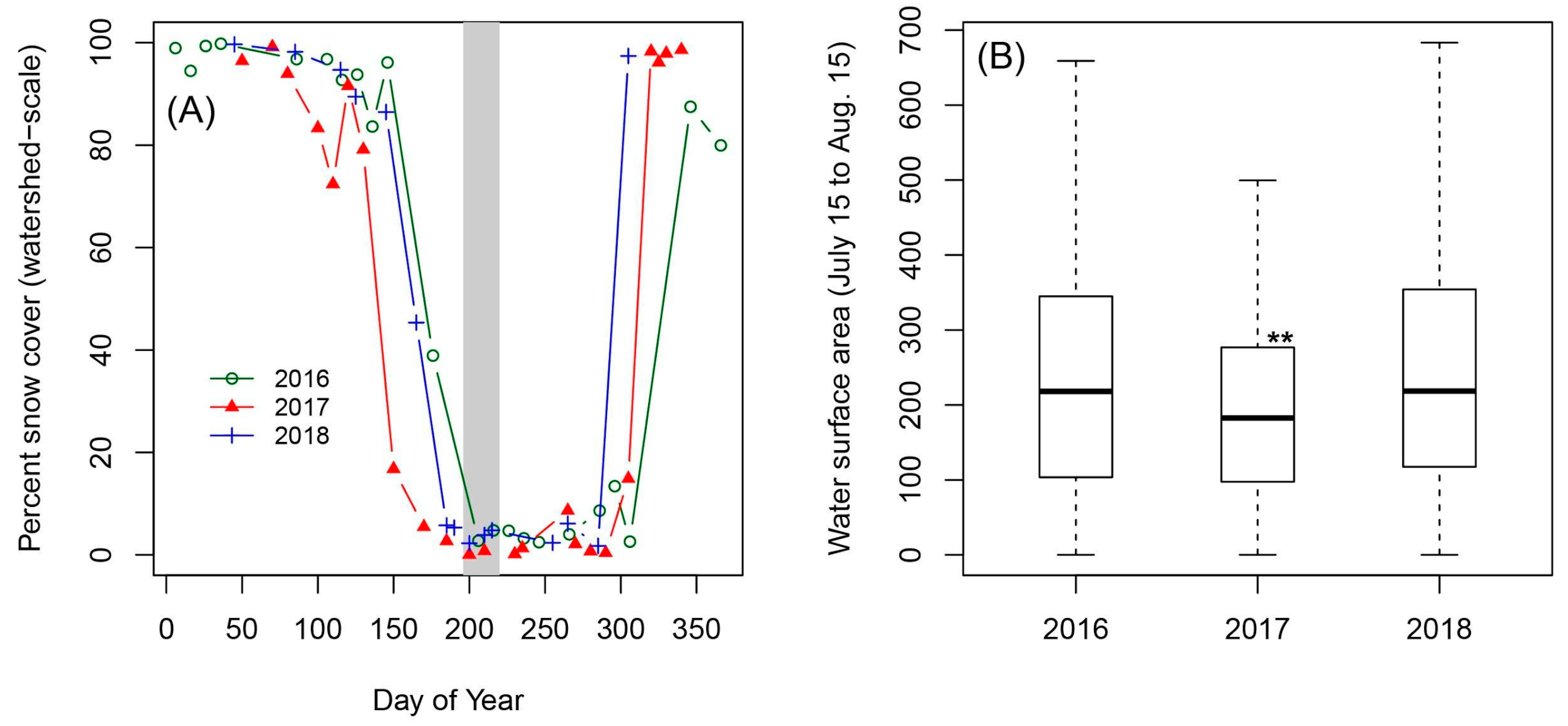
3.2. Characterization of Wetland Seasonal Hydrology (2016–2018)

Regardless of the threshold used to identify drought risk, 2017 stood out as the driest summer of the three-year study period (Figure 5). Summer 2016 was slightly drier than 2018 for thresholds below 60 m². Based on the error and uncertainty presented in Figure 4, we identified 25 m² as a potential drought risk threshold, meaning that we considered wetlands with less than 25 m² of estimated surface water (within the 20 m buffer zone corresponding to approximately 1300 m²) to be at risk of drought. Based on this threshold, of the 95 target wetlands, eight were dry in 2017, five were dry in 2016, and only one was dry in 2018 (Figure 5).

Regarding the persistence of mid-summer snowfields at the uppermost elevations of watersheds, in late-July and early-August snow covered 5 to 6% of watersheds in 2016 and 2018 and less than 1% of watersheds in 2017 (Figure 6). On average, watersheds became snow-free approximately three to four weeks earlier in 2017 compared to 2016 and 2018 (Figure 7A). In 2017, watersheds dropped below 20% snow cover on average by late-May, whereas in both 2016 and 2018, watershed snow cover did not decline rapidly until late-June (Figure 7B).

The three study years were highly contrasted in terms of March snowpack height and summer temperature and precipitation for the 1950–2250 m a.s.l. elevation band (Figure S5). With respect to the 30 year reference period, 2016 was close to average in terms of March snowpack depth, June–July GDD and June–July precipitation (Figure S5). The year 2017, however, was characterized by low snowpack high summer temperatures and average precipitation, with a 50 cm deficit in snowpack depth in March and a more than 100 °C surplus in June–July GDD. Last, snowpack depth in 2018 was 1 m above average, summer precipitation was well below average (−43 mm), and June–July GDD was well above average (+94 °C; Figure S5). Values extracted for wetlands exhibited the same inter-annual variability in snowpack and meteorological parameters (Figure S6).

For the July 15 to August 15 critical period, water surface area of target wetlands varied between 0 and 500–700 m² (Figure 6B). The mid-summer water surface area of wetlands was significantly lower in 2017 compared to 2016 and 2018 (Figure 6B), with a median decrease of 40–50 m² of surface water in 2017 (Figure 7B).

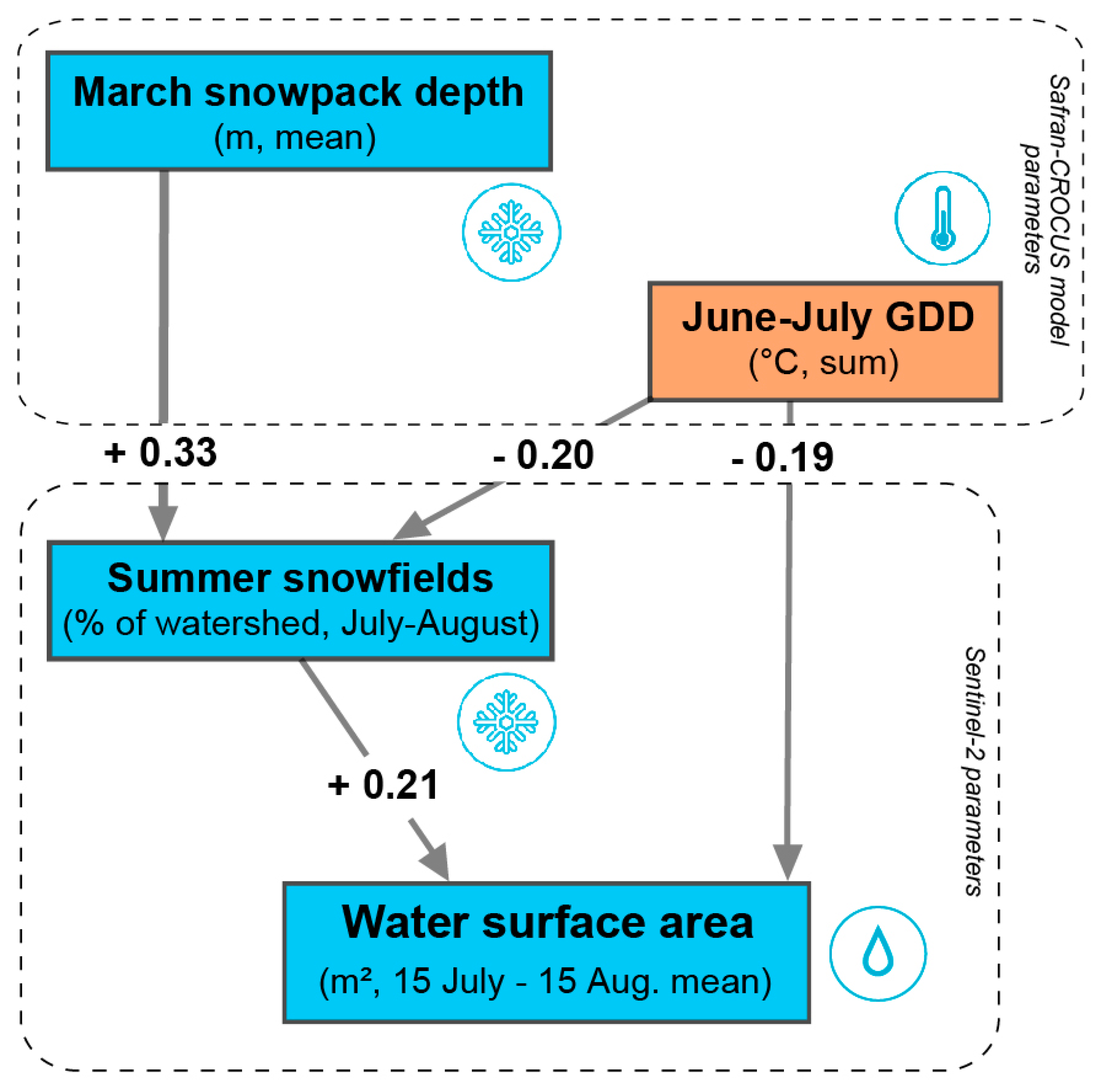
3.3. Structural Equation Modeling Results

Only one of the SEM models we tested was statistically acceptable (χ² p-value = 0.68, Table S1 Model 1A). This model also exhibited the lowest AIC value (16.76) compared to all other models (Table S1). Model 1A demonstrated a significant positive effect of March snowpack depth and a significant negative effect of June–July GDD on the persistence of Summer snowfields, followed by a significant positive effect of Summer snowfields and a negative effect of June–July GDD on Water surface area (Table S1, Figure 8). Interestingly, summer precipitation (June–July precip.) was not significantly related to Water surface area for any of the tested models, with the exception of Model 2B which exhibited a nearly significant negative relationship (p-value = 0.06, Path coefficient estimate of −0.16). Furthermore, Summer snowfields was the only measured snowpack parameter to have a significant effect on Water surface area, and local snow melt-out date of wetlands and at watershed snowmelt-out were not significant. We also tested for a direct effect of March snowpack height on Water surface area (results not shown), but did not observe a significant relationship or an improvement in model performance. Tested models explained between 4% and 11% of variance in Water surface area. Summary statistics for tested path models are provided in Table S1.

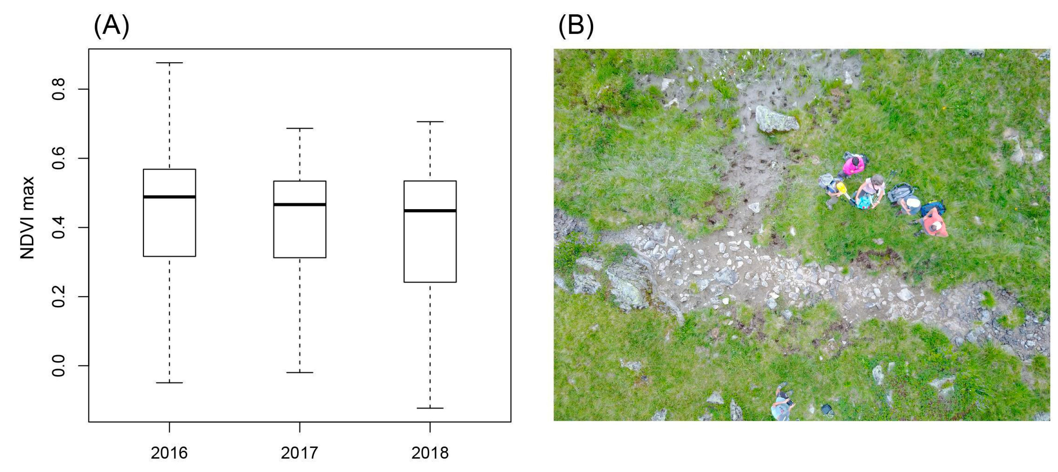
3.4. Observed Effects of Drought on Tadpole Development and Plant Biomass

In 2017, we observed the drying up of two monitored wetlands at the Loriaz site (Figure 1D) during a field visit on July 17. A subsequent field visit on August 3, 2017 confirmed the local mortality of frog tadpoles in these sites. Sentinel-2 estimates confirmed a lack of surface water for the July 17 date (Figure 4). We did not observe mid-summer drought and associated tadpole mortality for Loriaz sites in either 2016 or 2018. The 2017 drought occurred when tadpoles were in the process of developing from stage 3 to 4, which typically occurs during the critical drought-risk period from July 15 to August 15 for the Loriaz wetlands (Figure S7).

We did not observe a significant difference in peak NDVI (NDVI max) for wetland vegetation during the three years of the study (Figure 9A). Field observations and drone imagery indicated that even dry wetlands were surrounded by productive and lush vegetation, despite the lack of surface water (Figure 9B). We did not observe vegetation with a high degree of senescence during our mid-summer field observations of Loriaz wetlands in 2017.

4. Discussion

Our proposed use of Sentinel-2 imagery enables a novel approach for monitoring the seasonal hydrology of alpine wetlands and temporary pools, which constitute a ubiquitous and understudied feature of mountain landscapes with important implications for biodiversity and ecosystem services. We advocate for use of satellite imagery for automated monitoring of water surface area combined with field-based observations to quantify the consequences of drought on wetland plant and amphibian communities. In this paper, we provide examples of biotic responses to drought in terms of tadpole survival and plant biomass; however, further studies are needed in order to assess the population-level the effects of more frequent droughts on long-lived amphibian and plant species in a climate change context.

4.1. Methodological Limits & Perspectives

Our application of linear spectral unmixing provides a solution for mapping small and seasonally variable water bodies in alpine habitats, characterized by surface water extents of less than 100 m². Validation of spectral unmixing algorithm results demonstrated strong agreement with ground observations (Figure 4); however, with a degree of error that highlights certain methodological limitations. First, target wetlands were generally shallow (with a median water depth of 20 cm) and therefore exhibited spectral signatures that likely reflected a blend of surface water and underlying rocks, mud, and vegetation. This phenomenon is visually apparent in Figure 3D. Accordingly, we expect that the slight underestimation of water surface area for low water levels shown in Figure 4A results from blurred spectral signals in the case of extremely shallow water. One possible methodological improvement would be to include derived spectral indices such as the Bare Soil Index [42] in the spectral library used for endmember differentiation and spectral unmixing. This approach, i.e., including spectral index information in addition to band reflectance values, proved to be effective for multitemporal spectral unmixing and forest species mapping in the northeastern United States using NDVI in addition to Landsat 7 and 8 bands [28].

The difficulty of detecting extremely shallow surface water is an important consideration from an ecohydrological standpoint in the context of temporary alpine pools, given that field observations and previous studies indicate that small patches of shallow water between 10 and 15 cm of depth are sufficient for the growth and development of the common frog [43] as well as considerable zooplankton diversity [22]. Due to this uncertainty, for monitoring purposes we propose using a threshold of 25 m² (quantified within the 20 m buffer) below which drought is possible but difficult to detect with a high degree of certainty using our method. Accordingly, we propose that our method is sufficiently sensitive to quantify interannual variation in water surface area as well as drought risk for alpine wetlands distributed at the regional scale; however, field observations, potentially combined with higher resolution imagery, remain necessary in order to confirm the occurrence of drought for target ponds and pools.

We did not test the sensitivity of our results to spectral endmember selection, which is known to affect fractional cover estimates over time and space [44]. Given that our main target for this analysis was mapping fractional water cover, we assumed stationarity in the spectral properties of water over the course of the snow-free season from late spring to early fall. This assumption was supported by the consistently low residual error resulting from fraction estimates, particularly during the mid-summer season (Figure S2). Water spectral endmembers were defined in our case by selecting central pixels within lakes throughout the study area with low sediment concentration, which we consider to be a reproducible and consistent approach that could be utilized in other temperate mountain study areas. Should our multitemporal spectral unmixing approach be used for other applications such as mapping plant canopies or cover, which are influenced by species composition and are known to show highly variable spectral signals over course of the growing season [21], we recommend careful initial endmember selection using field spectroscopy as well as iteratively redefining spectral endmembers for each scene date [45].

4.2. Influence of Snowpack and Summer Climate on Wetland Hydrology

We relied on interannual variability in meteorological parameters during three highly contrasted study years as a means to assess the potential implications of climate change on alpine wetlands in our study area. The year 2017, which stood out as the driest of the three years considered, exhibited some of the most important climate changes currently underway in the Alps, including early snowmelt followed by the occurrence of summer heat waves (Figure S5). Our findings, which highlight an important regulatory role of snow cover parameters for the hydrology of alpine wetlands, align with results from the Canadian Rockies reporting that while alpine peat bogs are more resilient to drought due to increased soil water storage, mineral alpine wetlands and shallow pools with thin soils are likely to be more sensitive to interannual variability in climate [46]. It is important to point out that occasional drought occurrence is part of the usual functioning of semi-temporary basins in mountain environments, with wetland environments ranging along a continuum from permanent basins to temporary basins that dry shortly after snowmelt-out [11]. Our findings demonstrate that this continuum is sensitive to interannual variability in snow cover duration and summer temperature, with the implication that climate change could lead to a general shift toward increasingly dry and temporary alpine wetlands in the years ahead.

While we did not detect a positive effect of summer precipitation on midsummer water surface area, previous work has established the relevance of this parameter for the hydrology of alpine ponds and pools [11]. Given that the Chamonix valley is characterized by especially high average precipitation levels with respect to other alpine regions, it is also possible that summer precipitation has a stronger direct effect on water levels in drier systems such as the nearby southern French Alps. There may also be threshold effects, for example a minimum amount of received summer rainfall below which the risk of wetland drought dramatically increases, as was observed in the case of Australian wetlands during particularly hot and dry summers [16]. We also expect the effect of summer precipitation to depend in part on other climate parameters, and hypothesize that summer precipitation may become a critical hydrological input below certain snowpack levels or above certain temperatures. Last, while we did not test for the effect of geologic substrate on wetland hydrology or drought risk due to insufficient sample size across different bedrock types, we expect that the most important climate parameters may differ for example in limestone vs. granite watersheds. To address these questions, we recommend extending the remote sensing-based approach presented here, as well as field monitoring protocols of drought occurrence and amphibian phenology, at broader spatial scales in order to account for spatial non-stationarity in the relationships between meteorological parameters and wetland hydrology. Last, we propose that our method could be extended to estimate not only drought occurrence but also the duration and frequency of dry spells throughout the summer season.

4.3. Implications of Ongoing Climate Change for Alpine Wetland Habitat and Flora and Fauna

Twenty-first century scenarios of climate change for the European Alps predict ongoing and accelerating warming in future climate scenarios, including increasingly frequent and intense summer heat waves [47]. Summer precipitation is also expected to decrease by between 10 and 20% between now and 2050 in the Chamonix region depending on the scenario [48], suggesting that rainfall may become an increasingly important limiting factor in our study area in the years ahead. Furthermore, at 1500 m a.s.l., snow cover duration in the northern French Alps is expected to decrease with respect to the 1986–2005 reference period by approximately 3 weeks in 2030 and 4–5 weeks in 2050 [49]. Collectively, and in light of our findings, these predictions highlight increased drought risk for alpine wetlands in the coming years with strong implications for associated specialist flora and fauna. In terms of ecosystem services, reduced surface water and runoff linked to decreased snowpack, reduced summer rainfall and increased evapotranspiration, particularly in deglaciated watersheds, are projected to reduce summer stream flow and downstream water availability in alpine watersheds [50].

Our findings confirm the mortality of common frog tadpoles as a biotic response to drought, suggesting that consecutive years of dry conditions could affect the local viability of amphibian populations dependent on seasonally present water [22]. While, on the one hand, earlier snowmelt allows more time for tadpole development and growth in systems that are strongly limited by snow cover duration [51], on the other hand, reduced water availability associated with a thinner spring snowpack and smaller midsummer snow patches increases the risk of wetland drought during the summer (Figure 8 and Figure 9). A study conducted in the Rocky Mountains suggests that wetland habitat diversity and connectivity increases the resilience of frog populations to interannual climate variability, with shallow ephemeral sites being more favorable in wet and cold years and deeper and more permanent wetlands being more favorable to in warm and dry years [52]. Indeed the low R-squared values of our structural equation models highlight the remarkable habitat heterogeneity and complexity of alpine wetland pools, with highly variable characteristics despite similar climate conditions. Local characteristics including microtopography, bedrock, and soil heterogeneity and water runoff networks undoubtedly account for a large portion of unexplained variance in our model, and this habitat diversity may allow for certain pools to remain viable despite an overall decrease in water availability. Finally, while we quantified drought risk for wetlands considered as independent spatial entities, further work should seek to assess the potential effects of habitat configuration and spatial proximity of wetlands on amphibian survival and population dynamics in response to climate variability.

Our use of NDVI to quantify interannual responses of wetland plant biomass did not show any significant differences in plant productivity during the three study years, including for 2017 (Figure 9). Although additional fieldwork would be necessary to test this hypothesis, our initial observations (Figure 9B) suggest that soils adjacent to wetlands retain moisture and remain saturated even during periods of drought, and therefore can provide locally favorable conditions for plant growth when elsewhere plant growth might be hampered by moisture availability. Accordingly, wetlands could provide important refugia for above-treeline vegetation in the warmer and drier years ahead, particularly for subalpine to low-alpine vegetation, whose growth has been shown to be negatively affected by heat wave summers [53]. More frequent and sustained droughts could also lead to increases in the local abundance of generalist plant species at the expense of specialist hygrophile vegetation, which was observed in the Swiss Alps following 10 years of monitoring wetland plant community composition [13]. Given the combined threat to specialist wetland plant species posed by climate change and competitive exclusion by generalist plants, we recommend using Sentinel-2 not only for hydrological monitoring of snow cover and surface water, but also to detect potential changes in both plant biomass and shrub cover [21], in combination with repeated field surveys of wetland plant diversity.

5. Conclusions

Our work introduces and validates a novel application of multitemporal spectral unmixing, used to quantify the seasonal hydrology of alpine wetlands in the northern French Alps. We demonstrate that decreased snowpack and hot summers increase drought risk for alpine wetlands, with strong implications for the habitat requirements of specialist wetland flora and fauna. Our approach has the potential to be readily upscaled to systematically monitor above-treeline mountain pools at the regional scale for the duration of the Sentinel-2 satellite mission. We recommend combining remote sensing-based monitoring with systematic field observations to further enhance our method and to improve our understanding of ground-level responses of wetland plant communities and amphibian populations to ongoing climate changes.

References

1. Beniston, M. Mountain climates and climatic change: An overview of processes focusing on the European Alps. Pure Appl. Geophys. 2005, 162, 1587–1606. [Google Scholar] [CrossRef] [Green Version]
2. Gobiet, A.; Kotlarski, S.; Beniston, M.; Heinrich, G.; Rajczak, J.; Stoffel, M. 21st century climate change in the European Alps—A review. Sci. Total Environ. 2014, 493, 1138–1151. [Google Scholar] [CrossRef] [PubMed]
3. Corona-Lozada, M.C.; Morin, S.; Choler, P. Drought offsets the positive effect of summer heat waves on the canopy greenness of mountain grasslands. Agric. For. Meteorol. 2019, 276, 107617. [Google Scholar] [CrossRef]
4. Gardent, M.; Rabatel, A.; Dedieu, J.P.; Deline, P. Multitemporal glacier inventory of the French Alps from the late 1960s to the late 2000s. Glob. Planet. Chang. 2014, 120, 24–37. [Google Scholar] [CrossRef]
5. Huss, M. Extrapolating glacier mass balance to the mountain range scale: The European Alps 1900–2100. Cryosphere Discuss. 2012, 6, 1117–1156. [Google Scholar] [CrossRef]
6. Klein, G.; Vitasse, Y.; Rixen, C.; Marty, C.; Rebetez, M. Shorter snow cover duration since 1970 in the Swiss Alps due to earlier snowmelt more than to later snow onset. Clim. Chang. 2016, 139, 637–649. [Google Scholar] [CrossRef]
7. Steinbauer, M.J.; Grytnes, J.A.; Jurasinski, G.; Kulonen, A.; Lenoir, J.; Pauli, H.; Bjorkman, A.D. Accelerated increase in plant species richness on mountain summits is linked to warming. Nature 2018, 556, 231–234. [Google Scholar] [CrossRef]
8. Carlson, B.Z.; Corona, M.C.; Dentant, C.; Bonet, R.; Thuiller, W.; Choler, P. Observed long-term greening of alpine vegetation—A case study in the French Alps. Environ. Res. Lett. 2017, 12, 114006. [Google Scholar] [CrossRef]
9. Filippa, G.; Cremonese, E.; Galvagno, M.; Isabellon, M.; Bayle, A.; Choler, P.; Carlson, B.Z.; Gabellani, S.; Morra di Cella, U.; Migliavacca, M. Climatic Drivers of Greening Trends in the Alps. Remote Sens. 2019, 11, 2527. [Google Scholar] [CrossRef] [Green Version]
10. Rubel, F.; Brugger, K.; Haslinger, K.; Auer, I. The climate of the European Alps: Shift of very high-resolution Köppen-Geiger climate zones 1800–2100. Meteorol. Z. 2017, 26, 115–125. [Google Scholar] [CrossRef]
11. Wissinger, S.A.; Oertli, B.; Rosset, V. Invertebrate communities of alpine ponds. In Invertebrates in Freshwater Wetlands; Springer: Berlin/Heidelberg, Germany, 2016; pp. 55–103. [Google Scholar]
12. Hanzer, F.; Förster, K.; Nemec, J.; Strasser, U. Projected cryospheric and hydrological impacts of 21st century climate change in the Ötztal Alps (Austria) simulated using a physically based approach. Hydrol. Earth Syst. Sci. 2018, 22, 1593–1614. [Google Scholar] [CrossRef] [Green Version]
13. Moradi, H.; Fakheran, S.; Peintinger, M.; Bergamini, A.; Schmid, B.; Joshi, J. Profiteers of environmental change in the Swiss Alps: Increase of thermophilous and generalist plants in wetland ecosystems within the last 10 years. Alp. Bot. 2012, 122, 45–56. [Google Scholar] [CrossRef] [Green Version]
14. Blaustein, A.R.; Kiesecker, J.M. Complexity in conservation: Lessons from the global decline of amphibian populations. Ecol. Lett. 2002, 5, 597–608. [Google Scholar] [CrossRef] [Green Version]
15. Collins, J.P. Amphibian decline and extinction: What we know and what we need to learn. Dis. Aquat. Org. 2010, 92, 93–99. [Google Scholar] [CrossRef] [PubMed]
16. Stuart, S.N.; Chanson, J.S.; Cox, N.A.; Young, B.E.; Rodrigues, A.S.; Fischman, D.L.; Waller, R.W. Status and trends of amphibian declines and extinctions worldwide. Science 2004, 306, 1783–1786. [Google Scholar] [CrossRef] [PubMed] [Green Version]
17. Scheele, B.C.; Driscoll, D.A.; Fischer, J.; Hunter, D.A. Decline of an endangered amphibian during an extreme climatic event. Ecosphere 2012, 3, 1–15. [Google Scholar] [CrossRef]
18. Maltby, E.; Acreman, M.C. Ecosystem services of wetlands: Pathfinder for a new paradigm. Hydrol. Sci. J. 2011, 56, 1341–1359. [Google Scholar] [CrossRef]
19. Gascoin, S.; Grizonnet, M.; Bouchet, M.; Salgues, G.; Hagolle, O. Theia Snow collection: High-resolution operational snow cover maps from Sentinel-2 and Landsat-8 data. Earth Syst. Sci. Data 2019, 11, 493. [Google Scholar] [CrossRef] [Green Version]
20. Dedieu, J.P.; Carlson, B.Z.; Bigot, S.; Sirguey, P.; Vionnet, V.; Choler, P. On the importance of high-resolution time series of optical imagery for quantifying the effects of snow cover duration on alpine plant habitat. Remote Sens. 2016, 8, 481. [Google Scholar] [CrossRef] [Green Version]
21. Bayle, A.; Carlson, B.Z.; Thierion, V.; Isenmann, M.; Choler, P. Improved Mapping of Mountain Shrublands Using the Sentinel-2 Red-Edge Band. Remote Sens. 2019, 11, 2807. [Google Scholar] [CrossRef] [Green Version]
22. Tavernini, S.; Mura, G.; Rossetti, G. Factors influencing the seasonal phenology and composition of zooplankton communities in mountain temporary pools. Int. Rev. Hydrobiol. A J. Cover. All Asp. Limnol. Mar. Biol. 2005, 90, 358–375. [Google Scholar] [CrossRef]
23. Gao, B.C. NDWI—A normalized difference water index for remote sensing of vegetation liquid water from space. Remote Sens. Environ. 1996, 58, 257–266. [Google Scholar] [CrossRef]
24. Ozesmi, S.L.; Bauer, M.E. Satellite remote sensing of wetlands. Wetl. Ecol. Manag. 2002, 10, 381–402. [Google Scholar] [CrossRef]
25. Duffy, J.P.; Cunliffe, A.M.; DeBell, L.; Sandbrook, C.; Wich, S.A.; Shutler, J.D.; Myers-Smith, I.H.; Varela, M.R.; Anderson, K. Location, location, location: Considerations when using lightweight drones in challenging environments. Remote Sens. Ecol. Conserv. 2018, 4, 7–19. [Google Scholar] [CrossRef]
26. Sohn, Y.S.; McCoy, R.M. Mapping desert shrub rangeland using spectral unmixing and modeling spectral mixtures with TM data. Photogramm. Eng. Remote Sens. 1997, 63, 707–716. [Google Scholar]
27. Hostert, P.; Röder, A.; Hill, J. Coupling spectral unmixing and trend analysis for monitoring of long-term vegetation dynamics in Mediterranean rangelands. Remote Sens. Environ. 2003, 87, 183–197. [Google Scholar] [CrossRef]
28. Gudex-Cross, D.; Pontius, J.; Adams, A. Enhanced forest cover mapping using spectral unmixing and object-based classification of multi-temporal Landsat imagery. Remote Sens. Environ. 2017, 196, 193–204. [Google Scholar] [CrossRef]
29. De Asis, A.M.; Omasa, K.; Oki, K.; Shimizu, Y. Accuracy and applicability of linear spectral unmixing in delineating potential erosion areas in tropical watersheds. Int. J. Remote Sens. 2008, 29, 4151–4171. [Google Scholar] [CrossRef]
30. Huovinen, P.; Ramírez, J.; Gómez, I. Remote sensing of albedo-reducing snow algae and impurities in the Maritime Antarctica. ISPRS J. Photogramm. Remote Sens. 2018, 146, 507–517. [Google Scholar] [CrossRef]
31. Hagolle, O.; Huc, M.; Villa Pascual, D.; Dedieu, G. A multi-temporal and multi-spectral method to estimate aerosol optical thickness over land, for the atmospheric correction of FormoSat-2, LandSat, VENμS and Sentinel-2 images. Remote Sens. 2015, 7, 2668–2691. [Google Scholar] [CrossRef] [Green Version]
32. Hagolle, O.; Huc, M.; Desjardins, C.; Auer, S.; Richter, R. MAJA Algorithm Theoretical Basis Document. 2017. Available online: https://www.theia-land.fr/wp-content-theia/uploads/sites/2/2018/12/atbd_maja_071217.pdf (accessed on 4 April 2020). [CrossRef]
33. Dymond, J.R.; Shepherd, J.D. Correction of the topographic effect in remote sensing. IEEE Trans. Geosci. Remote Sens. 1999, 37, 2618–2619. [Google Scholar] [CrossRef]
34. Smith, M.O.; Ustin, S.L.; Adams, J.B.; Gillespie, A.R. Vegetation in deserts: I. A regional measure of abundance from multispectral images. Remote Sens. Environ. 1990, 31, 1–26. [Google Scholar] [CrossRef]
35. Dozier, J. Spectral signature of alpine snow cover from the Landsat Thematic Mapper. Remote Sens. Environ. 1989, 28, 9–22. [Google Scholar] [CrossRef]
36. Durand, Y.; Laternser, M.; Giraud, G.; Etchevers, P.; Lesaffre, B.; Mérindol, L. Reanalysis of 44 yr of climate in the French Alps (1958–2002): Methodology, model validation, climatology, and trends for air temperature and precipitation. J. Appl. Meteorol. Climatol. 2009, 48, 429–449. [Google Scholar] [CrossRef]
37. Durand, Y.; Giraud, G.; Laternser, M.; Etchevers, P.; Mérindol, L.; Lesaffre, B. Reanalysis of 47 years of climate in the French Alps (1958–2005): Climatology and trends for snow cover. J. Appl. Meteorol. Climatol. 2009, 48, 2487–2512. [Google Scholar] [CrossRef]
38. Vernay, M.; Lafaysse, M.; Hagenmuller, P.; Nheili, R.; Verfaillie, D.; Morin, S. The S2M meteorological and snow cover reanalysis in the French mountainous areas (1958–present). AERIS 2019. [Google Scholar] [CrossRef]
39. Grace, J.B.; Bollen, K.A. Interpreting the results from multiple regression and structural equation models. Bull. Ecol. Soc. Am. 2005, 86, 283–295. [Google Scholar] [CrossRef]
40. Shipley, B. Cause and Correlation in Biology: A User’s Guide to Path Analysis, Structural Equations and Causal Inference with R; Cambridge University Press: Cambridge, UK, 2016. [Google Scholar]
41. Grace, J.B. Structural Equation Modeling and Natural Systems; Cambridge University Press: Cambridge, UK, 2006. [Google Scholar]
42. Li, S.; Chen, X. A new bare-soil index for rapid mapping developing areas using Landsat 8 data. Int. Arch. Photogramm. Remote Sens. Spat. Inf. Sci. 2014, 40, 139. [Google Scholar] [CrossRef] [Green Version]
43. Gibbons, M.M.; McCarthy, T.K. Growth, maturation and survival of frogs Rana temporaria L. Ecography 1984, 7, 419–427. [Google Scholar] [CrossRef]
44. Dennison, P.E.; Roberts, D.A. Endmember selection for multiple endmember spectral mixture analysis using endmember average RMSE. Remote Sens. Environ. 2003, 87, 123–135. [Google Scholar] [CrossRef]
45. Liu, S.; Bruzzone, L.; Bovolo, F.; Du, P. Unsupervised multitemporal spectral unmixing for detecting multiple changes in hyperspectral images. IEEE Trans. Geosci. Remote Sens. 2016, 54, 2733–2748. [Google Scholar] [CrossRef]
46. Mercer, J.J. Insights into Mountain Wetland Resilience to Climate Change: An Evaluation of the Hydrological Processes Contributing to the Hydrodynamics of Alpine Wetlands in the Canadian Rocky Mountains. Ph.D. Thesis, University of Saskatchewan, Saskatoon, SK, Canada, 2018. [Google Scholar]
47. Jacob, D.; Petersen, J.; Eggert, B.; Alias, A.; Christensen, O.B.; Bouwer, L.M.; Georgopoulou, E. EURO-CORDEX: New high-resolution climate change projections for European impact research. Reg. Environ. Chang. 2014, 14, 563–578. [Google Scholar] [CrossRef]
48. Cremonese, E.; Carlson, B.; Filippa, G.; Pogliotti, P.; Alvarez, I.; Fosson, J.P.; Ravanel, L.; Delestrade, A. AdaPT Mont-Blanc Rapport Climat: Changements Climatiques Dans le Massif du Mont-Blanc et Impacts Sur Les Activités Humaines. Report Written in the Context of the AdaPT Mont-Blanc Projet and Financed by the European Union (Alcotra France-Italy 2014–2020). November 2019, p. 101. Available online: http://espace-mont-blanc.com/asset/rapportclimat.pdf (accessed on 4 April 2020).
49. Verfaillie, D.; Lafaysse, M.; Déqué, M.; Eckert, N.; Lejeune, Y.; Morin, S. Multi-component ensembles of future meteorological and natural snow conditions for 1500 m altitude in the Chartreuse mountain range, Northern French Alps. Cryosphere 2018, 12, 1249–1271. [Google Scholar] [CrossRef] [Green Version]
50. Huss, M.; Bookhagen, B.; Huggel, C.; Jacobsen, D.; Bradley, R.S.; Clague, J.J.; Vuille, M.; Buytaert, W.; Cayan, D.R.; Greenwood, G.; et al. Toward mountains without permanent snow and ice. Earth’s Future 2017, 5, 418–435. [Google Scholar] [CrossRef]
51. Corn, P.S. Amphibian breeding and climate change: Importance of snow in the mountains. Conserv. Biol. 2003, 17, 622–625. [Google Scholar] [CrossRef] [Green Version]
52. McCaffery, R.M.; Maxell, B.A. Decreased winter severity increases viability of a montane frog population. Proc. Natl. Acad. Sci. USA 2010, 107, 8644–8649. [Google Scholar] [CrossRef] [Green Version]
53. Cremonese, E.; Filippa, G.; Galvagno, M.; Siniscalco, C.; Oddi, L.; di Cella, U.M.; Migliavacca, M. Heat wave hinders green wave: The impact of climate extreme on the phenology of a mountain grassland. Agric. For. Meteorol. 2017, 247, 320–330. [Google Scholar] [CrossRef]
Figure 1. (A) Locator map displaying the study area in the Chamonix valley, France. (B) Photo of a typical alpine pond habitat in the Mont-Blanc massif. (C) Map of the 22 alpine watersheds (above 1800 m a.s.l.) and the 95 alpine wetlands considered in this analysis. (D) Inset map showing the locating of four wetlands visited weekly during the summer months to monitor the phenology of common frog (Rana temporaria) populations and periodically to survey wetland surface water extent.
Remotesensing 12 01959 g001
Figure 2. Spectral signatures of target endmembers, identified using 50 cm resolution aerial photographs and extracted from a Sentinel-2A image on August 3, 2016. (A) Mean reflectance values for spectral endmembers for the 10 utilized Sentinel-2 bands. (B) Mean PCA coordinates of spectral endmembers, showing 95% confidence intervals.
Remotesensing 12 01959 g002
Figure 3. Example time series of fractional snow and water cover for a select wetland extracted from Sentinel-2 imagery in 2017 (A) and 2018 (B). Solid point values are result of fractional estimates resulting from a simple extract of spectral values for the GPS point. The hollow point in panel (A) indicates the fractional estimate for a 20 m buffer around the GPS point, which was the method used for all subsequent analysis. Panels (C,D) show drone images of the targeted wetland in July, 2017, and June, 2018. The red point indicates the GPS point used for field monitoring and image analysis, the blue rectangle shows the overlapping Sentinel-2 pixel, and the diameter of the 20 m buffer used to estimate surface water in the vicinity of target wetlands.
Remotesensing 12 01959 g003
Figure 4. Validation of Sentinel-2 based estimates of water surface area relative to visual ground-based estimates carried out by volunteers. Values are based on a grid of nine 10 × 10 m pixels centered on the GPS point of a target wetland (see Figure S1). (A) Mean water surface area observed on the ground compared to mean water surface area estimated using Sentinel-2, with error bars representing 95% confidence intervals. (B) Total water surface area observed on the ground compared to total water surface area estimated using Sentinel-2. The dashed line represents a 1:1 relationship while the solid line represents a line of best fit using linear standardized major axis regression. Point symbols correspond to do different visit dates in the field, which were coordinated with the passage of the satellite. MAE = mean absolute error.
Remotesensing 12 01959 g004
Figure 5. Number of dry wetlands (N = 95) depending on the threshold used to identify drought risk. Values are based on sum of water surface area within a 20 m buffer around wetlands or approximately a 1300 m2. For monitoring purposes, we propose utilizing a threshold of 25 m2 given the uncertainty of the method presented in Figure 4B.
Remotesensing 12 01959 g005
Figure 6. Mid-summer images for (A) 2016, (B) 2017, and (C) 2018 showing the spatial distribution of persistent snowfields, watershed boundaries, and wetlands for a portion of the study area. Although cirrus clouds are present in panel (B), masked pixels did not cover snowfield areas.
Remotesensing 12 01959 g006
Figure 7. (A) Mean percent snow cover for 22 watersheds >1800 m a.s.l. for 2016, 2017, and 2018; the gray rectangle indicates the July 15 to August 15 period considered for drought-risk. (B) Average water surface area, applying the 20 m buffer, for alpine wetlands during the July 15 to August 15 period in 2016, 2017, and 2018; ** denotes a significant difference in water surface area values between 2017 and the other years according to a Pairwise Wilcoxon signed rank test: 2017 vs. 2016, p-value = 0.001; 2017 vs. 2018, p-value = 0.004, 2016 vs. 2018, not significant).
Remotesensing 12 01959 g007
Figure 8. Structural equation model results for the retained model (Table S1, Model 1A), linking hydrological (blue) and meteorological (orange) parameters to interannual (2016–2018) variability in the mid-summer water surface area of wetlands. Line thickness is proportional to the values of path coefficient estimates. Boxes with dashed outlines indicate variables measured using the Safran-CROCUS atmosphere-snowpack model, and spatial variables measured using Sentinel-2 satellite imagery.
Remotesensing 12 01959 g008
Figure 9. (A) Boxplots of maximum Normalized Difference Vegetation Index (NDVI) values observed for wetlands during the July 15 to August 15 period for the three study years. (B) Drone photograph of a dried out wetland in 2017, showing lush vegetation despite the dry conditions.
Remotesensing 12 01959 g009