A Developed Siamese CNN with 3D Adaptive Spatial-Spectral Pyramid Pooling for Hyperspectral Image Classification


1
Aerospace Information Research Institute, The Institute of Remote Sensing and Digital Earth (RADI), Chinese Academy of Sciences (CAS), Beijing 100101, China
2
School of Electronic, Electrical and Communication Engineering, University of Chinese Academy of Sciences (UCAS), Beijing 100101, China
*
Author to whom correspondence should be addressed.
†
These authors contributed equally to this work.
Remote Sens. 2020, 12(12), 1964; https://0-doi-org.brum.beds.ac.uk/10.3390/rs12121964
Submission received: 21 April 2020
/
Revised: 17 May 2020
/
Accepted: 10 June 2020
/
Published: 18 June 2020
(This article belongs to the Special Issue Machine Learning and Pattern Analysis in Hyperspectral Remote Sensing)
Abstract
:Since hyperspectral images (HSI) captured by different sensors often contain different number of bands, but most of the convolutional neural networks (CNN) require a fixed-size input, the generalization capability of deep CNNs to use heterogeneous input to achieve better classification performance has become a research focus. For classification tasks with limited labeled samples, the training strategy of feeding CNNs with sample-pairs instead of single sample has proven to be an efficient approach. Following this strategy, we propose a Siamese CNN with three-dimensional (3D) adaptive spatial-spectral pyramid pooling (ASSP) layer, called ASSP-SCNN, that takes as input 3D sample-pair with varying size and can easily be transferred to another HSI dataset regardless of the number of spectral bands. The 3D ASSP layer can also extract different levels of 3D information to improve the classification performance of the equipped CNN. To evaluate the classification and generalization performance of ASSP-SCNN, our experiments consist of two parts: the experiments of ASSP-SCNN without pre-training and the experiments of ASSP-SCNN-based transfer learning framework. Experimental results on three HSI datasets demonstrate that both ASSP-SCNN without pre-training and transfer learning based on ASSP-SCNN achieve higher classification accuracies than several state-of-the-art CNN-based methods. Moreover, we also compare the performance of ASSP-SCNN on different transfer learning tasks, which further verifies that ASSP-SCNN has a strong generalization capability.

1. Introduction
Hyperspectral sensors typically acquire images across hundreds of spectral bands with rich spatial information, which makes hyperspectral images (HSI) become essential data sources to deal with the heterogeneous and mixed landscape. Therefore, the HSI classification method is widely applied in material analysis [1,2], environmental detection [3,4], precision agriculture [5,6] and other application fields [7,8]. Therefore, it is an important task to develop a classification method of hyperspectral images with high precision and strong generalization. Deep convolutional neural networks (CNN) have attracted much attention due to their excellent performance in hyperspectral image classification tasks [9,10,11,12,13]. However, such methods usually exhibit two common issues: (1) How to develop a high-precision deep learning model with limited labeled samples. (2) How to develop a deep learning model with strong generalization for classification tasks on different hyperspectral datasets.
In more recent years, because CNN can extract low, mid, and high-level spatial features, various CNN-based deep learning models have been applied to HSI classification with limited labeled samples. In order to adequately train CNN in the case of limited labeled samples, different strategies have been introduced to either augment the training set or reduce the parameters of the network. For instance, Jacopo Acquarelli et al. proposed a method using CNNs and data augmentation to classify all unlabeled pixels of the given HSI [14]. They augmented the training data by propagating the label of pixels in the training set to its neighbors and trained a simple single-layer CNN with a tailored loss function. Hyungtae Lee et al. [15] have presented a CNN architecture to jointly optimize the spectral and spatial information of HSI. They have leveraged the residual structure to overcome sub-optimality in CNN performance caused primarily by limited amounts of training samples. Liu Zhu et al. [16] have explored a generative adversarial network (GAN) based on CNN for HSI classification. The proposed GAN can generate virtual samples that are used with real training samples to fine-tune the GAN’s discriminative CNN. Their experimental results have proven the effectiveness of using virtual samples to improve the generalization capability of the discriminative CNN. The pieces of literature mentioned above are based on the original labeled sample set to generate pseudo-labeled samples, multi-scale inputs, or virtual samples, respectively. Such strategies for augmenting training samples are helpful to alleviate the problems caused by limited labeled samples. However, such strategies can only add a finite amount of information for training deep learning model, because of the augmented samples are similar to the real labeled samples. Moreover, the deep CNN models with a single sample as input do not fully explore the relation feature between samples, which limits the discrimination ability of the CNN supervised classifier.
To fully explore the potential of CNN, CNN with sample-pairs as input have been applied for HSI classification. Wei Li et al. [17] proposed a pixel-pair method to significantly increase the number of training samples, ensuring that the advantage of CNN can be proposed. Their experimental results demonstrate that CNN trained with pixel-pair has excellent classification performance. Bing Liu et al. [18] proposed a supervised deep feature extraction method based on Siamese CNN to improve the performance of HSI classification. The experiment results of this method show that the Siamese CNN with sample-pair as input can extract robust discriminative features for HSI classification. Taking sample-pairs as input, not only can significantly increase the number of training samples, but also the CNN trained by sample-pairs has stronger discrimination ability than the CNN with a single sample as input. In views of the above advantages of taking sample-pairs as input, Siamese CNN has promising potential in HSI classification with limited labeled samples. However, the first Siamese neural network [19] was designed for binary classification tasks, and it could not meet the requirements of multi-classification tasks for HSI. To overcome this problem, a Siamese CNN is developed for multi-classification tasks with limited labeled samples.
It is worth noting that we have proposed a developed Siamese CNN (ES-CNN) in [20], which not only take advantage of sample-pairs as input but also can be directly applied to multi-classification tasks. Its experiments show that the proposed method has great potential for HSI classification. However, the proposed method in [20] only extracts spectral information by a one-dimensional convolutional network (1D-CNN), while it ignores spatial information. In this paper, to fully explore the potential of both spatial and spectral information, the core of our architecture is the use of the three-dimensional convolutional network (3D-CNN) throughout the network. More importantly, to make the proposed method have better generalization capability, we consider a new Siamese CNN for classifying different HSIs with the different number of bands.
One of the most common ways to analyze the generalization capability of deep learning models is to discuss the transfer learning framework of deep learning models for different HSI classification tasks. Hyungtae Lee et al. [21] have devised a classification approach that pre-trains a network on multiple source datasets that differ in their hyperspectral characteristics and then fine-tunes on a target dataset. Their experimental results show that the pre-training network is beneficial to improve the classification accuracy, and the datasets of different HSI sensors are useful for the pre-training. Ke Li et al. [22] have proposed a new hyperspectral classification method based on transfer learning and the deep learning method. They used a hyperspectral dataset that is similar to the target dataset to pre-training the deep learning network. The experimental results show that transfer learning can obtain better classification accuracy in a shorter amount of time when the source data and the target data are obtained from the same sensor. However, due to the various type of hyperspectral sensors, different HSIs may contain a different number of bands. The pre-trained network needs to be able to tackle different HSIs with a different number of bands. For this problem, the most direct solution is to unify the number of bands of resource datasets and target dataset by using dimensionality reduction [23,24]. This approach, based on dimensionality reduction, may lose some valuable information. Notably, [25,26] employ adaptive average pooling to adjust the size of output features to a fixed size. With the adaptive average pooling, they can transfer a CNN model between heterologous HSI datasets. To solve the problem that deep learning model require a fixed-size input, Kaiming HE et al. proposed the spatial pyramid pooling (SPP) for visual recognition in 2015 [27]. By equipping a network with SPP layer, the network can generate a fixed-length representation regardless of input size. To adapt to heterologous HSIs classification, we equip 3D ES-CNN with a new pooling strategy, called 3D adaptive spatial-spectral pyramid pooling (3D-ASSP).
In this paper, we propose a Siamese CNN with 3D adaptive spatial-spectral pyramid pooling, called ASSP-SCNN, which can be transferred to heterologous HSI datasets without unifying the number of bands of resource datasets and target dataset. In contrast to the first Siamese CNN [28] and the ES-CNN [20], our proposed network not only can fully explore the potential of both spatial and spectral information, but also allows us to feed samples with varying sizes or scales during training into the proposed network. Training our network with variable-size samples increases scale-invariance and reduces over-fitting. To verify the classification performance and generalization capability of ASSP-SCNN, we conduct two sets of experiments: the classification experiments without pre-training and the classification experiments with pre-training. In the classification experiments without pre-training, we train the model from scratch on the target dataset to analyze the classification performance of ASSP-SCNN for HSI with limited labeled samples. In the experiment with pre-training, we propose a transfer learning framework based on ASSP-SCNN for verifying the classification performance of pre-trained ASSP-SCNN on a source dataset after transferring to a target dataset.
This work focuses on how to adapt Siamese CNN to HSI multi-classification task with limited labeled samples. The proposed ASSP-SCNN and its corresponding transfer learning framework can achieve state-of-the-art performance in terms of classification accuracy. The main contributions of this paper are as follows:
- (1)
- To the best of our knowledge, this is the first that 3D adaptive spatial-spectral pyramid pooling layer (3D-ASSP) is employed for HSI classification. We propose a 3D pyramid adaptive pooling layer based on developing the SPP [27] and adaptive average pooling [25,26]. By equipping a network with 3D-ASSP layer, the network can generate a fixed-length representation regardless of 3D input size as well as extract multi-level 3D features to increases its scale-invariance.
- (2)
- A developed Siamese CNN for HSI multi-classification is proposed. We equip a Siamese CNN with 3D-ASSP layer to obtain a new Siamese CNN, called ASSP-SCNN. The proposed ASSP-SCNN consisting of more than ten layers, can be directly applied to HSI multi-classification. Furthermore, it can be fully trained only with train samples of target HSI without any auxiliary dataset. Interestingly, different from the first Siamese CNN [28] and the ES-CNN [20], the proposed network can not only explore the potential of both spatial and spectral information for HSI classification but also allow us to put three-dimensional samples with varying sizes or scales into the network. In other words, the ASSP-SCNN can classify heterologous HSI datasets without unifying their number of bands.
- (3)
- The generalization of the proposed ASSP-SCNN is thoroughly analyzed. We proposed an ASSP-SCNN-based transfer learning framework for different HSI classification tasks to verify the generalization capability of ASSP-SCNN. We transfer the ASSP-SCNN between different HSI datasets captured by the same sensor or different sensors. We compare the performance of the ASSP-SCNN and its transfer learning framework from classification accuracy, training time and other aspects, revealing that the proposed ASSP-SCNN has strong generalization performance.
The remainder of this paper is as follows. Section 2 provides an introduction to related work, including SCNN [19] and SPP [27]. Section 3 presents the details of our proposed classification framework, including ASSP-SCNN and the implementation details of transfer learning based on ASSP-SCNN. Section 4 introduces the datasets, experimental setups, and discuss the experiential results. Finally, we present conclusions about our work and point out future work in Section 5.
2. Materials
2.1. Labeling Strategy for Samples Pairs
Li et al. [17] proposed labeling strategy for pixel-pairs that maps a pixel-pair set to a multi-class label set. In this paper, we apply this strategy for labeling sample-pairs, the basic idea of which is described as follows. Consider a hyperspectral data set with M three-dimensional labeled samples, denoted as , where d represents the number of bands and represents the spatial window size of a sample. The class label of a 3D sample is denoted as , which is equal to the label of the center pixel of and C represents the number of classes. Let denote the number of available labeled samples in the class and satisfy . We randomly select two sample from X to form a sample-pair . Then the labeling strategy for is: If the two samples belong to the same class, the label of the is same as . Otherwise, the label of is . The formula is shown by the following Equation (1).
According to the above labeling strategy for sample-pair, the labeled sample-pair set contains classes, and its size is M times the size of X. More specifically, we randomly select twice from X and get two samples , if then . Therefore, the size of the labeled sample-pair set is .
2.2. End-to-End Siamese Convolutional Neural Network
In [20], we proposed an end-to-end Siamese convolutional neural network (ES-CNN) for HSI multi-classification tasks based on spectral information. In contrast to the original Siamese convolutional neural network (SCNN) [19], which is a classifier suitable for binary classification tasks, ES-CNN is a classifier suitable for multi-classification tasks. We show the architectures of ES-CNN and the original SCNN are in Figure 1.
A significant improvement from original SCNN to ES-CNN is that ES-CNN is equipped with a fully connected network to replace the energy function and output layer in the original SCNN. The output layer of ES-CNN contains multiple neurons, which enables it to deal with multi-class classification tasks directly. As the change of network topology, compared with SCNN, ES-CNN’s labeling strategy of sample-pair, the way of generating classification map and loss function are introduced as follows.
We are applying the labeling strategy of sample-pair proposed in [17] (similar to Section 2.1). After labeling the sample-pair set by this strategy, the labeled sample-pair set contains one more class than the original training set. Specifically, if the training set contains C classes, the labeled sample-pair set contains classes, and the extra class label indicates that these two samples of a sample-pair do not belong to any same class.
As the input of ES-CNN is a sample-pair, we apply a neighborhood voting strategy to determine the class label of a center pixel finally. The underlying assumption of this strategy is that the central pixel has high probability of belonging to the same class as its neighbor pixels. Assuming a neighborhood is chosen, Figure 2 illustrates the voting strategy. Concretely, for a pixel to be classified, we first select a neighborhood of the pixel to get 24 pixel-pairs. Then we feed these pixel-pairs into the trained network to predict their labels. Given the predicted labels, we first exclude the pixel-pairs do not belong to the same class, then the label with the most significant number of votes is selected as the center pixel’s class label.
As the output of ES-CNN contains multiple neurons, we proposed a new version of the cross-entropy loss function in [20] in Equations (2) and (3).
where n is batch size, a decimal between 0 and 1. The term is the standard hinge loss. is the label of pixel-pair, and is one-hot label of . is the predicted value of the i-th pixel-pair, and is the one-hot label of . is a regularization to guarantee the accuracy of HSI classification. is the weight coefficient.
2.3. Spatial Pyramid Pooling and Adaptive Pooling
In 2015, Kaiming HE et al. [27] equipped a network with spatial pyramid pooling to eliminate the requirement that deep CNN requires a fixed-size input. They also pointed out that the fixed-size constraint comes only from the fully connected layers, while convolutional layers do not require a fixed-size input and can generate feature maps of any size. In other words, for the classification method based on CNN, we can remove the fixed-size constraint of the network if we generate a fixed-size/length outputs to feed into the fully connected layers. To the best of our knowledge, both of spatial pyramid pooling layer [27] and adaptive pooling layer (https://pytorch.org/docs/master/nn.functional.html#adaptive-avg-pool3d) can pool features to generate a fixed-size representation from arbitrarily sized input.
Specifically, the adaptive pooling strategy was first designed in the PyTorch (https://pytorch.org/) library. According to different pooling operations, adaptive pooling has two specific implementations: adaptive maximum pooling and adaptive average pooling. The particularity of adaptive pooling lies in that as long as we give the input data and the output size of adaptive pooling, it can automatically help us to calculate the size of kernel, padding and stride. Specifically, consider an input size of the adaptive pooling is , we want to generate an feature after pooling, then the parameters of the corresponding pooling layer can be decided by the following Equation (4).
where the floor is a function that rounds down to the nearest integer. In practice, it is convenient to use an adaptive pooling layer to generate a fixed-size representation because its parameters include only the size of the output.
Spatial pyramid pooling technology can generate a fixed-length output regardless of input size as well as use multi-level spatial bins to generate a robust output to object deformation. Figure 3 shows the structure of a CNN with a spatial pyramid pooling layer. The CNN equipped with a spatial pyramid pooling layer between the convolutional layers and the fully connected layers. Three levels concatenate the fixed-sized/length representation generated by the SPP pooled outputs with the size of , and , respectively. Here c is the filter number of the convolutional layer before SPP. Therefore, by equipping with a spatial pyramid pooling layer, A CNN can generate multi-level features to improve the scale-invariance of the CNN.
3. Methods
Inspired by the above, we propose a Siamese CNN with a 3D adaptive spatial-spectral pyramid pooling, called ASSP-SCNN, for HSI classification with limited labeled samples. Figure 4 shows the architecture of ASSP-SCNN, which consists of four parts: input, feature extraction module, metric module and output. We note that ASSP-SCNN has several remarkable properties for deep CNNs:
The input of ASSP-SCNN is 3D sample-pair. By feeding the 3D sample-pair into the network, it can fully explore the potential of both spatial and spectral information between samples. Moreover, this sample-pair strategy can quadratically increase the amount of network input to satisfy the training of deep networks.
The feature extraction of ASSP-SCNN contains a 3D adaptive pyramid pool layer, which allows us to feed samples with varying sizes or scales during training and can extract multi-level feature with fixed-size.
The metric module of ASSP-SCNN consists of four fully connected layers, which takes the features of 3D samples pair as input, and its output layer contains multiple neurons. Equipped with this metric module, ASSP-SCNN can measure the similarity of sample-pairs as well as can deal with HSI multi-classification directly.
We divide this section into three parts. The first part introduces the 3D adaptive spatial-spectral pyramid pooling, the second part introduces the classification framework of ASSP-SCNN in detail, and the third part introduces the transfer learning framework based on ASSP-SCNN to prepare for the subsequent analysis of the ASSP-SCNN’s generalization.
3.1. 3D Adaptive Spatial-Spectral Pyramid Pooling
To remove the fixed-size input requirement of 3D CNN, we proposed a 3D adaptive spatial-spectral pyramid pooling (ASSP) strategy. Specifically, we add an ASSP layer on the top of a 3D CNN’s last convolutional layer. The ASSP layer pools feature and generate fixed-size output, which is then fed into the fully connected layers. An example of a CNN structure with 3D adaptive spatial-spectral pyramid pooling is shown in Figure 5.
As shown in Figure 5, the adaptive pyramid pool layer contains a multi-level pyramid to generate several spatial-spectral bins. In each spatial-spectral bin, we pool the responses of each filer of the equipped network’s last convolutional layer. The input of ASSP layer is the output of the last convolutional layer with size , where c is the number of filters in the last convolutional layer and the output each feature map of such filter has the size of . The output of the ASSP layer is a fixed-dimensional vector with size , where M is the number of spatial-spectral bins. The fixed-dimensional vector is the input of a fully connected layer.
In our experiment, we constructed a three-level pyramid with different scales of , and , respectively. In Section 2.3, we pointed out an advantage of adaptive pooling that we give the input data and the output size of adaptive pooling in PyTorch, and it can automatically help us to calculate the size of kernel, padding and stride. By the convenient of applying adaptive pooling, we respectively apply a 3D adaptive average pooling layer to pool the input of ASSP for each level. Moreover, we set the output sizes of the three-level 3D adaptive average pooling layer to , and , respectively. Therefore, we flatten the outputs of these adaptive pooling layers into one-dimensional vectors and concatenate them together, resulting in spatial-spectral bins. The proposed pooling strategy apply 3D adaptive pooling to generate fixed-sized features for each level of multi-level pyramid pooling, so we called this pooling as ‘adaptive spatial-spectral pyramid pooling’.
3.2. Siamese CNN with 3D Adaptive Spatial-Spectral Pyramid Pooling Layer
As indicated previously, ES-CNN [20] takes sample-pair as input to significantly increases the number of training samples, ensuring that the advantage of CNN can be offered. 3D adaptive spatial-spectral pyramid pooling can remove the fixed-size input requirement of 3D CNN. Inspired by this, we developed a Siamese CNN with 3D adaptive spatial-spectral pyramid pooling layer (ASSP-SCNN). As shown in Figure 4, the architecture of the proposed ASSP-SCNN contains three parts: sample-pair construction, feature extraction and metric module. In the remaining portion of this subsection, we will successively introduce the three parts in detail.
3.2.1. Sample-Pair Construction
Consider an HSI dataset containing N labeled pixels denoted as in pixel space , where d is the number of bands contained in the HSI dataset. Let be the class label of and C is the number of classes contained in the dataset. We split dataset X into the training set , and the testing set with no intersection between these two sets. For any pixel , we take it as the center pixel to intercept a spatial neighborhood with size as a 3D sample . Here the size of is , and the label of is .
In the training stage, we first randomly select two pixels, and from the training set . We respectively take these two pixels to intercept two 3D samples and , forming a 3D sample-pair . The labeling strategy for sample-pair is shown in Section 2.1. Please note that ASSP-SCNN can be fed with samples with varying sizes or scales during training. Therefore, for the two selected pixels, and , we can generate multiple sample-pairs according to different spatial window sizes. Consider K different spatial window sizes, the sample-pair set for training ASSP-SNN is as Equation (5).
In the testing stage, for each pixel of the testing set , we take it as the center to intercept a 3D sample and generate a sample-pair . Therefore, consider a certain spatial window size , the sample-pair set for testing is in Equation (5):
where the set contains sample-pairs and the class label of is same as . In contrast to the neighborhood voting strategy of ES-CNN [20] in Section 2.3, the generation strategy of testing sample-pairs in this section do not need post-processing, so ASSP-SCNN can achieve a faster efficiency when generating a classification map.
3.2.2. Feature Extraction
After the sample-pair construction, we fed a sample-pair into a feature extraction to extract multi-level spatial-spectral features of the sample-pair. The proposed feature extraction is 3D-CNN with an adaptive spatial-spectral pyramid pooling layer. Figure 6 illustrates the architecture of our feature extraction module, which consists of four convolutional blocks, a 3D ASSP layer and three fully connected layers. For a given sample-pair containing two 3D samples, and , we fed the two samples into the feature extraction to generate two features and with a same size.
As shown in Figure 6, we propose a feature extraction with a 3D ASSP layer, which takes 3D sample-pair as input. The size of each sample is , where b is the batch size of the input, is the spatial window size of the sample and d is the number of the sample’s band. The feature extraction consists of four 3D CNN blocks, a 3D ASSP layer and three fully connected layers. Each 3D CNN block is a concatenation of a convolution layer, a batch normalization layer, a ReLU activation layer and a pooling layer. More concretely, the first 3D CNN contains 3D convolutional filters with size , followed by a batch normalization layer, a ReLU activation layer and a max-pooling layer with a stride of . First, we fed a 3D sample into the first 3D CNN block , generating a tensor with size , where 51 is an integral part of , and with padding. We fed the output tensor of into the second 3D CNN block , and by this block-to-block feature extraction we get an output of the fourth 3D CNN block whose size is . Then we fed the output of into a 3D ASSP layer, which contains a three-level pyramid with output size , and , respectively. Therefore, the output size of the 3D ASSP layer is . Finally, we fed the output of 3D ASSP layer into a fully connected network resulting in a feature with size .
3.2.3. Metric Module
We fed two features of a sample-pair extracted by feature extraction into a fully connected network, which can not only measure the similarity of the input features but also generated the probability values that the sample-pair belongs to each class. We call this fully connected network as the metric module. Figure 7 illustrates the architecture of our metric module, whose input is the concatenation between a sample-pair’s features and after feature extraction. The output layer contains C+1 neuron nodes, where the first C nodes represent the probability that the sample-pair belongs to class t, , and the node value represents the probability that the two samples in the sample-pair are not similar.
According to Figure 6, the output of feature extraction is a tensor with size . Therefore, the first fully connected layer of our metric module contains 1000 neurons in Figure 7. It is worth noting that all fully connected layers equipped with ReLU activate function except the output layer equipped with the Softmax activate function. By the Softmax activate function, the output of our metric module which satisfies . Here is a scalar value ranges from 0 to 1, representing the probability values that belongs to label t. For any sample-pair , we fed it into ASSP-SCNN to generate the probability values, which can be described as the following mathematical Equation (7).
where is the metric module with parameters , represents the operation of feature concatenation, and is the feature extraction with parameters W. We assume the mini-batch size is B and use the mean square error (MSE) loss to train ASSP-SCNN based on the fact that ASSP-SCNN conceptually produces continuous similarity scores produces continuous instead of discrete 0 or 1 values. Our loss function is of the form:
where is the sample-pair, which is composed of two 3D samples and a label , and its one-hot label is . We apply Adam optimizer to minimize the loss function during training. Notably, ASSP-SCNN consists of feature extraction and metric module, then we employ two Adam optimizers to train the two modules, respectively. The employ of such two optimizers refers to the original code of the relation network [11]. The optimization process can be expressed as follows.
3.3. APP-SCNN Based Transfer Learning
To verify the generalizability of ASSP-SCNN, we propose a transfer learning framework based on ASSP-SCNN for HSI classification. Consider that hyperspectral images usually contain hundreds of bands, and the number of bands is much larger than RGB images or multi-spectral images. In this case, applying models pre-trained in other fields may lead to a loss of spectral information. Therefore, we only analyze the model transfer between HSI datasets. The flowchart of our transfer learning framework is shown in Figure 8, which consist of two part: a pre-training part and a fine-tune part. Here we introduce the transfer learning strategy in detail.
3.3.1. Pre-Training Strategy
The pre-training of ASSP-SCNN in source HSI dataset is shown in Figure 8a, which consists of multiple 3D-CNN layers, an ASSP layer and multiple fully connected layers. We construct training sample-pair set from a source HSI dataset to train the ASSP-SCNN. Then an output with size is produced by the ASSP-SCNN, which represents the probability values that the input sample-pair belongs to each class. Here is the number of classes in the source dataset. There are two key points that should be noticed.
Source dataset and target dataset can be collected by the different HSI sensors. Hyungtae Lee et al. [21] observed that pre-training of the network has its advantage in achieving better performance when deeper networks are required and transfer learning between HSIs from different sensors is effective. Therefore, we proposed a transfer learning classification framework based on ASSP-SCNN for HSIs classification from different sensors, to analysis the generalizability of ASSP-SCNN. Our transfer learning experiments include source dataset for pre-training and the target dataset for fine-tuning from the same sensor, as well as from different sensors.
At the stage of sample-pair construction, it is not necessary to unify the number of bands contained in the source dataset and target dataset 3D samples. To transfer the pre-trained model on a source dataset to target dataset with the different number of bands, scholars usually choose to unify the number of bands of the source dataset and the target dataset at the stage of sample-pair construction [23,24]. Such solutions have a risk of losing useful spectral information during the sample-pair construction. To solve the above problem, we equip a Siamese CNN with a 3D ASSP layer to adapt the different size of 3D sample-pair as input. Therefore, the number of bands of sample-pair can be consistent with the original HSIs for pre-training or fine-tuning.
3.3.2. Fine-Tuning Strategy
As shown in Figure 8b, we transfer the entire pre-trained model except for the output layer to the network built for target HSI dataset as initialization. We then fine-tune the transferred part and the new output layer on target HSI dataset. Two key points should be noticed in fine-tuning as follows.
The parameters of the last layer (output layer) of the pre-trained model are not transferred. Because the source dataset and target dataset may contain a different number of classes, and thus we need to change the number of neurons in the output layer of pre-trained model to achieve multi-classification of the target dataset. In this case, we only replace the output layer of the pre-trained model to generate a new ASSP-SCNN for the target dataset. Therefore, we transfer the entire pre-trained model except for the output layer to the network built for target HSI dataset as initialization. Please note that we randomly initialize the output layer of the ASSP-SCNN for the target HSI.
During fine-tuning, both the transferred part and the new output layer are trained with the same learning rate by using Adam optimizer. Yenan Jiang et al. pointed out that the random initialization part of the network should use the same learning rate as the transferred pat during fine-tuning. And lower learning rate means narrower parameter space in HSI so that the ability of network structure cannot be fully used [26]. Therefore, in the fine-tuning stage of transfer learning based on ASSP-SCNN, we adapt a uniform learning rate to fine-tune the whole network for target HSI.
4. Results and Discussion
We evaluate the proposed ASSP-SCN by HSI classification experiments on three benchmark datasets. Furthermore, we implement our network using the Python language and the PyTorch library. The codes of our network are running on a computing workstation with two Intel Xeon E5-2620v4 CPUs and four NVIDIA TITAN XP GPUs. We only used one GPU for each experiment.
4.1. Data Description and Experiment Design
4.1.1. Data Description
To evaluate the performance and generalization of ASSP-SCNN, we applied ASSP-SCNN and its transfer learning framework to three benchmark HSI datasets. The three datasets are collected from different heterogeneous and mixed landscapes by two different HSI sensors. The details of the three datasets are listed in Table 1. Specifically, the Indian Pines is a medium spatial resolution image (20 m), two-third of which belong to agriculture, and the remaining one third are forest or other natural perennial vegetation. Since the scene is captured in June, some of the corns, crops, soybeans are less than 5% coverage. Its ground-truth contains 16 classes and is not all mutually exclusive. Pavia University dataset (PaviaU) is collected from urban areas with a high spatial resolution (1.3 m). Although its ground-truth contains nine classes, PaviaU also covers heterogeneous and mixed landscapes. For instance, it contains two different types of asphalt (Asphalt and Bitumen). The Salinas is characterized by high spatial resolution (3.7 m), which is between Indian Pines and PaviaU. Moreover, Salinas contains 16 classes including vineyard fields, bare soils and vegetation.
4.1.2. Experiment Design
For the proposed ASSP-SCNN, the two critical motivations of our experiments are to answer the two questions as follows: (1) If the ASSP-SCNN without pre-training is sufficient for HSI classification with limited labeled samples. (2) Whether the ASSP-SCNN with pre-training on source dataset with limited labeled samples has strong generalization.
Experiment Design of classification without pre-training: In the experiments of classification without pre-training, we split each target dataset into three subsets: training pixel set, validation pixel set and testing pixel set. For all data sets, we randomly select 180 labeled pixels for training, 20 labeled pixels for validation, and the rest for testing. For Indian Pines, if the class has less than 400 pixels, then we select 40% labeled pixels for training, 10% labeled pixels for validation, and the rest for testing. The number of pixels for constructing training sample-pairs, validation sample-pair and testing sample-pair, are listed in Table 2, Table 3 and Table 4 as follows.
For constructing the input of ASSP-SCNN, it is necessary to extract pixels from the above-partitioned set to form the 3D sample-pair set. In Table 5, we list the size of training 3D sample-pairs set, validation 3D sample-pairs set and testing 3D sample-pairs set of each dataset. Concretely, we describe the construction strategy for the sample-pair set in Section 3.2.1.
To be specific, for the training 3D sample-pair set: we conduct random selection twice to obtain two pixels. By the two selected pixels, we can construct a 3D sample-pair with a spatial window size . Consider a training pixel set with size M, and given K different spatial window size, then the size of 3D sample-pairs for training is .
For the validation 3D sample-pair set and testing 3D sample-pairs: the class label of sample-pair need to be decided during validation or testing. Therefore, consider a pixel need to classify, we construct a 3D sample with spatial window size . Then we obtain a 3D sample-pair based on the 3D sample . By feeding the 3D sample-pair into the trained ASSP-SCNN, we can obtain the label of the pixel . Therefore, the size of the validation 3D sample-pair set is the same as that of the validation pixel set, and the size of the testing sample-pair set is the same as that of the testing pixel set.
In experiments for classification without pre-training, we apply the training 3D sample-pair set to training ASSP-SCNN, the validation 3D sample-pair set to tuning hyperparameters of ASSP-SCNN, and the testing 3D sample-pair set to evaluate the performance of trained ASSP-SCNN. To evaluate the performance, we chose a range of criteria, including overall accuracy (OA), class-specific accuracy, and Kappa coefficient as indicators of performance against other CNN-based methods. Therefore, under the above evaluation criteria, we compare the classification results of our ASSP-SCNN to the results obtained using a multiple classifier systems based on SVM and random feature selection (SVM-RFS) [29], deep multi-grained cascade forest (dgcForest) [30], one-dimensional CNN (1D-CNN) [9], a deep CNN for learning pixel-pair features (CNN-PPF) [17], a five-layer CNN for classification (C-CNN) [31], a classification method combining Siamese CNN and support vector machine (SVM+SCNN) [18], and a deep few-shot learning method combined with SVM (DFSL+SVM) [23] on all the three datasets.
Experiment Design of classification with pre-training: We designed the transfer learning classification experiments based on ASSP-SCNN to evaluate the generalization of ASSP-SCNN and the necessity of pre-training. In the experiments of classification without pre-training, we obtain three trained ASSP-SCNN for the above three HSI datasets. For each ASSP-SCNN trained with a source dataset, we transfer its parameters to initialize two new ASSP-SCNN for the other two target dataset, respectively. After initializing the ASSP-SCNN for target dataset, we fed 3D sample-pairs constructed on target dataset to fine-tune the ASSP-SCNN for target HSI classification. Two key points should be noticed in experiments with pre-training as follows.
The target dataset is divided into two part: training pixel set and testing pixel set. Indeed, we have tuned the hyperparameters of ASSP-SCNN on source dataset in the experiments of classification without pre-training. Therefore, in experiments with pre-training, we only need the training pixel set for fine-tuning the transfer learning model, and testing pixel set for evaluating the performance of the transfer learning model.
To evaluate the performance of transfer learning based on ASSP-SCNN for HSI classification with limited labeled pixels. In the fine-tuning stage, we selected five labeled pixels set with different size on target dataset to construct 3D sample-pairs for fine-tuning the transfer learning framework, respectively. Specifically, we select labeled pixels for each class on target dataset to obtain a pixel set for fine-tuning the transferred network. Here we set to 25, 50, 100, 150 and 200, respectively, and the obtained five labeled pixels set satisfy that . After selecting the labeled pixel set for fine-tuning, we apply the remain labeled pixels of the target dataset for testing the transferred network.
4.2. Parameter Tuning
In contrast to ordinary 3D-CNN, there are two critical points of the proposed ASSP-SCNN: (1) we equip feature extraction with an ASSP layer to remove the fixed-size input requirement of 3D CNN. (2) we apply a fully connected network to measure the similarity of the input and classify the label of input. Therefore, we do not discuss the effects of the number of layers contained ASSP-SCNN, the size of a convolutional kernel, and the number of neurons contained each layer in this paper. We analysis the hyperparameters of ASSP-SCNN, including the learning rate of the network, the decay coefficient of the learning rate, size of the ASSP layer and the spatial window size of input 3D sample-pair.
4.2.1. Learning Rate and its Decay Coefficient
Learning rate can significantly affect the training performance since it determines the convergence speed in the procedure of backpropagation [18,32]. We train models with different learning rate to find the optimum initial learning rate from . Based on the performance in the validation set, we set the learning rate to for the three HSI datasets. Moreover, we employ Adam [33] as the optimizer and set the momentum to 0.9, which is widely used for training deep network on image classification and action recognition tasks [25,34,35,36]. By observing the change of training loss and validation loss during training, we set the decay coefficient of the learning rate to 0.5 for every 50,000 batches, and the upbound of the batch is 300,000. We set the batch size to 59 according to the GPU memory of our computing workstation. As the convergence rate of each dataset is not the same during training, we set an early stopping strategy that if for more than 5000 batches the validation loss is no longer falling, the training process of the network is stopped.
4.2.2. Effect of the Pyramid Size of 3D ASSP Layer
As shown in Figure 5, a 3D ASSP layer contains an L-level pyramid, and the output of each level is a tensor with size . In this paper, we analyze the case that the size of the output in each level satisfies . By this case, for a 3D ASSP layer contains an L-level pyramid, we denote the size of the 3D-ASSP as which means the output of i-th level pyramid is . Therefore, the output of the 3D ASSP layer is a 1D tensor with length if the input of the 3D ASSP layer is a tensor with size .
The most important advantage of the ASSP-SCNN is that it contains a 3D ASSP layer to remove the fixed-size input requirement of 3D CNN. The size of the 3D ASSP layer is a hyper-parameter which affects the performance of the proposed model. To demonstrate the effect of different size of 3D ASSP layer, and choose an optimal for our comparing experiments with other CNN-based methods, taking PaviaU dataset as an example, we equip ASSP-SCNN with seven different ASSP layer with size and , respectively. We show the statistical results of ASSP-SCNN on PaviaU dataset with the different candidate ASSP layers of in Table 6.
From Table 6, we can observe that the ASSP-SCNN with 3-level pyramid achieves higher overall accuracy (OA) (99.048%) and Kappa coefficient (0.987) than ASSP-SCNN with the 1-level pyramid or 2-level pyramid. This result indicates that the multi-level pyramid pooling is beneficial to improve the classification accuracy of the proposed model. Comparing the three experiment results obtained by the ASSP-SCNN with a 1-level pyramid with sizes , respectively, we can see that the ASSP-SCNN with ASSP layer size of achieves higher OA (98.504%) and Kappa coefficient (0.980) than the ASSP-SCNN with ASSP layer size of or . The main reason for this is that the feature extracted by the ASSP layer size of contains more useful spectral-spatial information for classification. Comparing the results by ASSP-SCNN with the 1-level pyramid and 2-level pyramid, we observe that the ASSP-SCNN with an ASSP layer size of achieve higher accuracy than other ASSP layers. Moreover, the experiment results obtained by ASSP size of is better than , and it may be that the features extracted by the two levels are too similar to weaken the separability between different classes, as the PaviaU dataset has a high spatial resolution.
4.2.3. Effect of the Spatial Window Size of the Input
In our ASSP-SCNN, we can take any size of 3D sample-pair as input and the spatial window size of 3D sample-pair will affect the classification performance of ASSP-SCNN. To analyze the influence of the spatial window size of training sample-pairs, we set the size of ASSP to and train ASSP-SCNNs with different combinations of spatial window size of 3D sample-pairs to find the optimum combination of spatial window sizes from . For example, taking the spatial window size combination of 3D sample-pairs to training ASSP-SCNN, we take each training pixel as the center pixel to intercept a spatial neighborhood with sizes , and , respectively, forming three 3D samples. Therefore, for training the pixel set of ASSP-SCNN, we can construct a training sample-pair set according to the spatial window size combination . In Table 7, we present the statistical results of training ASSP-SCNN for PaviaU dataset based on a constructing 3D sample-pair set according to different spatial window size combinations.
From Table 7, the ASSP-SCNN, which was trained by multiple spatial window sizes, can achieve higher OA and Kappa coefficient than the ASSP-SCNN trained by single spatial window size. By comparing the results generated by the ASSP-SCNN with the single spatial widow size, we observe that the ASSP-SCNN with the spatial window size , achieve higher OA (99.048%) and Kappa coefficient than the ASSP-SCNN with the other single spatial window sizes from . Based on this comparison, we implement three different experiments that we train ASSP-SCNN by feeding the constructing 3D sample-pair sets according to different spatial window size combinations and , respectively. Therefore, we observe that the training ASSP-SCNN with the spatial window size combination , achieve higher OA (99.512%) and Kappa coefficient (0.993) than the training ASSP-SCNN with the other two with spatial window combinations. These facts reveal that training ASSP-SCNN with multiple spatial window sizes can improve the classification performance of ASSP-SCNN.
4.3. Comparison to Previous Classifiers
To demonstrate the effectiveness of the proposed ASSP-SCNN, we compare with seven previous methods including SVM-RFS [29], dgcForest [30], 1D-CNN [9], CNN-PPF [17], C-CNN [31], SVM+SCNN [18], and DFSL+SVM [23]. These comparison methods include two hard classification methods (SVM-RFS and dgcForest) and five CNN-based methods. The main reason for selecting these two hard classification methods is to reveal the performance gap between ASSP-SCNN and the hard classifiers. There are two main reasons for choosing the five competing CNN-based methods: on the one hand, the five methods and ASSP-SCNN belong to deep learning method based on CNN, which applied for HSI classification with limited labeled pixels. Here the five methods include deep learning based on 1D-CNN, 3D-CNN and Siamese CNN, respectively, which are relevant to the structure of ASSP-SCNN to ensure an omnidirectional comparison. On the other hand, the experiment results of the five methods generated on a relatively uniform experimental background. To be specific, the five methods provide classification results on the three datasets, and the number of labeled pixels for training is the same for each dataset. In the uniform experimental background, four key points should be noticed in the comparing experiments as follows.
The experimental data distribution of our ASSP-SCNN is consistent with the experiments of the comparing methods [9,17,18,23,29,30,31]: To ensure the fairness of the comparison, we apply the ASSP-SCNN for classification on Indian Pines, PaviaU and Salinas, respectively. Moreover, we keep the size of the training pixel set, and testing pixel set same between our ASSP-SCNN and the comparing methods for each dataset. Accurately, for PaviaU and Salinas datasets, Table 2, Table 3 and Table 4 show the number of labeled pixels for training, validation and testing the ASSP-SCNN. As shown in Table 2, Table 3 and Table 4, for each class, we apply 180 labeled pixels to training ASSP-SCNN, this number of training pixels is less than comparing methods (200 per class). Moreover, the compared results of dgcForest [36] obtained by randomly selecting 10% labeled samples per class for training model and the rest samples for testing. According to the experimental results given in the reference [30], we do not list the experimental results obtained by dcgForest on Indian Pines with nine classes in Table 8. For Indian Pines, we train our ASSP-SCNN with nine classes to be consistent with the comparing methods. We apply 180 labeled pixels per class for training ASSP-SCNN, 20 labeled pixels per class for validation, and the rest pixels per class for testing. If any hyperparameters are involved, we select the optimal ones to ensure the performance of ASSP-SCNN was fully exploited. For instance, we set the size of the ASSP layer in ASSP-SCNN to , and the spatial window size combination of sample-pair to .
We only show the statistical comparison results of ASSP-SCNN and the comparing methods: Since the codes of comparing methods [9,17,18,23,29,30,31] are not online, and we only provide a comparison between the statistical classification results generated by ASSP-SCNN and the statistical classification results generated by the reference methods. To be specific, we evaluate the classification performance by three commonly used quantitative criteria: class-specific accuracy, OA and Kappa coefficient. We show the comparisons of the three criteria on different datasets in Table 8, Table 9 and Table 10, respectively. It is worth noting that we did not show the comparison results of SVM+SCNN [18] in Table 10 since the reference did not present the classification result of SVM+SCNN on Salinas dataset.
Form Table 8, Table 9 and Table 10, we observe that ASSP-SCNN achieves higher OA and Kappa coefficient than the comparison methods on all three target datasets in general. Compared with the two hard classifiers, the overall accuracies generated by ASSP-SCNN on the three datasets are increased by at least 5%, especially on the Indian Pines dataset, the OA generated by ASSP-SCNN is increased by nearly 10%. Specifically, for the Indian Pines dataset, the OA obtained by ASSP-SCNN is 99.17%, which is 0.13% higher than the highest OA (SVM+SCNN, 99.04%) obtained by the seven comparing methods. From the perspective of class-specific accuracy, we observed that the ASSP-SCNN does not achieve the highest class-specific accuracies for all classes. However, it achieves the class-specific accuracies of all classed are not less than 98.44%. Similar situations happen to the other two target datasets. According to the statistical comparisons of classification results on the three datasets, it demonstrates that the ASSP-SCNN without pre-training achieves competitive performance for HSI classification with limited labeled pixels, compared to the seven state-of-the-art methods.
We present the classification results generated by ASSP-SCNN on Indian Pines with 16 classes: In the above comparison experiments, we only listed the classification results generated by ASSP-SCNN on Indian Pines with nine classes to consistent with the comparing methods. However, the Indian Pines dataset contains 16 classes, so we present the classification results obtained by ASSP-SCNN on Indian Pines with 16 classes in Table 11.
From Table 11, we observe that ASSP-SCNN achieves high class-specific accuracy for the class containing limited labeled pixels. For instance, the first class (No. 1) of Indian Pines dataset provides 18 labeled pixels to training ASSP-SCNN, then its class-specific accuracy is 97.96%. The similar situation happens to the other classes. Meanwhile, the class-specific accuracy per class is no less than 90.91%, the OA is 97.848%, and the Kappa coefficient is 0.975. The experiment results reveal that ASSP-SCNN without pre-training can achieve high accuracy for HSI classification with limited labeled pixels.
We show the classification maps generated by ASSP-SCNN on the above three HSI datasets with different spatial window sizes in Figure 9, Figure 10, Figure 11 and Figure 12: Since we can feed 3D HSI sample-pair with arbitrary spatial window size to ASSP-SCNN, we choose different spatial window size to construct testing sample-pairs in the testing phase, from the candidate spatial window size set . To demonstrate the effect of the spatial window size of input sample-pairs for testing, we present the classification result maps and the relevant overall accuracies obtained by ASSP-SCNN on the three datasets with different spatial windows sizes.
From Figure 9, Figure 10, Figure 11 and Figure 12, we can see that the classification maps are more similar to the relevant ground-truth map as increasing the spatial window size of the testing sample-pairs for each target HSI dataset. Moreover, the overall accuracies obtained by ASSP-SCNN on the target dataset also increase gradually. The phenomena are consistent with the statistical result in Table 7, which is the analysis for the effect of different spatial window sizes in the training phase. Concretely, taking Salinas dataset as an example, we can see that the classification accuracies obtained by ASSP-SCNN with the above candidate spatial window size set are 93.44%, 96.30%, 97.53% and 98.15% respectively. The similar increases of classification accuracy happen on the other two target datasets, which reveals the following fact: In the stage of applying the trained ASSP-SCNN for testing or generating the classification result map, we need to select an appropriate spatial window size for constructing the sample-pair. In the case of HSI classification, we recommend selecting the optimal spatial window size in the parameter tuning stage. Furthermore, note that we can obtain a better classification result map by weighted voting between the classification maps generated by ASSP-SCNN with different spatial window sizes.
4.4. Transfer Learning Based on ASSP-SCNN
The above experiments show that ASSP-SCNN without pre-training can achieve competitive performance for the three HSI classification tasks, compared to the seven state-of-the-art methods. However, the generalization of ASSP-SCNN is still an unknown problem. To further reveal the generalization of ASSP-SCNN, we propose a transfer learning framework based on ASSP-SCNN. In particular, we have trained an ASSP-SCNN for each dataset in the experiments without pre-training. Now for each dataset, we transfer the pre-trained ASSP-SCNN to the other two datasets. We have shown the flowchart of our transfer learning framework in Figure 8, which consist of two part: a pre-training part and a fine-tune part. During the fine-tuning phase, the hyperparameters of the ASSP-SCNN for target HSI dataset are the same as the ASSP-SCNN without pre-training.
Taking the Salinas dataset as a source dataset, we transfer the pre-trained ASSP-SCNN to the ASSP-SCNN for another target HSI dataset classification including PaviaU dataset and Indian Pines dataset, respectively. The transferred ASSP-SCNN is trained on Salinas dataset in the above experiments of classification without pre-training. On the target dataset, we randomly selected and 200 labeled pixels per class for constructing the 3D sample-pairs for fine-tuning the transferred ASSP-SCNN, respectively. Moreover, the rest labeled pixel in the target dataset for testing. It is worth noting that we have trained two ASSP-SCNN for Indian Pines dataset in the experiments of classification without pre-training, one with nine classes and another one for Indian Pines dataset with 16 classes. Therefore, in the experiments of transfer learning, we view the Indian Pines dataset as two datasets with the different number of classes, which are consistent with the experiments of classification without pre-training and denoted as Indian Pines_9 and Indian Pines_16.
Table 12 lists the overall accuracies obtained by the ASSP-SCNN-based transfer learning framework between the three datasets. We bolded the overall accuracies which are higher than the results in experiments of classification without pre-training. For instance, we bolded the overall accuracy obtained by ASSP-SCNN-based transfer learning from Indian Pines with 16 classes, which is 99.614% higher than the value 99.52% obtained by the ASSP-SCNN without pre-training (Seen in Table 9). The bolded values indicate that the trained ASSP-SCNN has strong generalization on different datasets. In addition, we observed that the transfer learning framework presented three trends in HSI classification tasks:
The ASSP-SCNN shows strong generalization even though the number of labeled pixels for fine-tuning is small, in the case where we transfer an ASSP-SCNN from a source dataset with low-spatial-resolution to the target dataset with high spatial resolution. For instance, in the experiment of transfer learning from Indian Pines (its spatial resolution is 20 m) to PaviaU (its spatial resolution is 1.3 m) or Salinas (its spatial resolution is 3.7 m), the overall accuracies obtained by the fine-tuned ASSP-SCNN on target dataset is higher than 92%, even though we apply 25 labeled pixels per class for fine-tuning. In contrast, in the experiments of transfer learning from PaviaU or Salinas to Indian Pines, the overall accuracies obtained by fine-tuning ASSP-SCNN with 25 labeled pixels per class are less than 84%.
The main reason for the above phenomenon is that the information intensity between images with medium-low-spatial-resolution and high spatial resolution is different, and thus the ASSP-SCNN model pre-trained on different HSIs performs inconsistently. On the one hand, compared with high-spatial-resolution images (such as PaviaU or Salinas), there are more mixed pixels in medium–low-spatial-resolution images (such as Indian Pines) since a single pixel of such image covers a larger area. On the other hand, the high-spatial-resolution image contains sufficient spatial information, such as apparent geometric features and texture structure. Therefore, the ASSP-SCNN trained on medium-low-spatial-resolution images is suitable for the more complex classification tasks than those trained on high-spatial-resolution images. So, in our experimental results, the ASSP-SCNN pre-trained on Indian Pines shows a more robust generalization than those pre-trained on the other two HSI datasets.
The ASSP-SCNN-based transfer learning is valid between the HSI datasets captured by different sensors. Although the PaviaU and Salinas are captured by different HSI sensors, the overall classification accuracy achieved by fine-tuning ASSP-SCNN from the PaviaU to Salinas with the different number of labeled pixels is 92.682%, 93.833%, 96.954%, 97.823% and 98.209%, respectively. The similar situation has occurred in the experiments of ASSP-SCNN-based transfer learning from Salinas or Indian Pines to PaviaU.
Moreover, taking PaviaU as target dataset and the number of samples for fine-tuning is not more than 100 per class, the ASSP-SCNN pre-trained on Indian Pines_9 achieves higher OA than ones pre-trained on Indian Pines_16. The main reason for this pheromone may be that Indian Pines_9 contains the same number of classes as PaviaU and the transferred ASSP-SCNN do not need to replace the output layer in the fine-tuning stage. When the number of samples for fine-tuning is not less than 150 per class, the ASSP-SCNN pre-trained on Indian Pines_16 shows a more robust generalization than ones pre-trained on Indian Pines_9. This phenomenon may be that the ASSP-SCNN pre-trained on Indian Pines_16 contains more diverse information than ones pre-trained on Indian Pines_9, and the information can be fully transferred to the target classification model in the case of sufficient fine-tuning samples.
The ASSP-SCNN-based transfer learning present excellent classification performance between the datasets with the different number of classes on the same region. In the experiments of transfer learning from Indian Pines with nine classes to Indian Pines with 16 classes, the obtained overall accuracies are not less than 93.648% (25 labeled pixels per class for fine-tuning). In the experiments of ASSP-SCNN-based transfer learning from 16 classes to nine classes on Indian Pines, the overall classification accuracy obtained was not less than 97.840% (100 labeled pixels per class for fine-tuning). The phenomenon indicates that ASSP-SCNN has a strong generalization for the HSI classification on the same dataset with a different number of classes.
Moreover, we observed that the overall classification accuracies obtained by the proposed transfer learning framework on a target dataset are increasing gradually as the number of labeled pixels for fine-tuning increases. In the experiments of using 200 labeled pixels per class for fine-tuning, the overall accuracies are close to that obtained by ASSP-SCNN without pre-training in Table 8, Table 9 and Table 10. Compare to the results in Table 8, Table 9 and Table 10, the ASSP-SCNN-based transfer learning present excellent classification performance than the comparison methods [9,17,18,23,31] under the same number of labeled pixels for training and testing.
4.5. Time Comparison Between ASSP-SCNN Without Pre-Training and ASSP-SCNN Based Transfer Learning
Generally, the convergence time of the CNN-based transfer learning model in the fine-tuning phase is less than the same CNN model without pre-training in the training phase. To reveal the time required for ASSP-SCNN-based transfer learning, TABLE 12 lists the training time of ASSP-SCNN without pre-training and the fine-tuning time of ASSP-SCNN-based transfer learning on the three datasets. The statistical time is the time to spend on training or fine-tuning of the proposed model on a target dataset when the overall accuracy is higher than a given value. To specific, the given values for Indian Pines with nine classes, Indian Pines with 16 classes, PaviaU and Salinas are set to be 98.6%, 97.5%, 99.4% and 97.9%, respectively. To record the first time that the model achieves the OA higher than the given values, we designed experiments to test every 5000 batch during the training or fine-tuning process, Therefore, the statistical time including the training (fine-tuning) time and several testing time. The bolded values in Table 13 indicate the fine-tuning of the pre-trained model takes longer time than training the model without pre-training on the target set. Please note that the time for generating Indian Pines_9, IndianPines_16, PaviaU and Salinas classification maps on the trained ASSP-SCNN is 1 minute 6 seconds, 1 minute 6 seconds, 13 minutes 3 seconds, 13 minutes 22 seconds, respectively. In terms of time efficiency, we found that the transfer learning framework based on ASSP-SCNN has the following two properties:
For transfer learning task that transfers the model from high-spatial-resolution dataset to low-spatial resolution dataset, the performance of ASSP-SCNN-based transfer learning framework is worse than the ASSP-SCNN without pre-training. The bolded time values in Table 13 shows the fine-tuning time of transfer learning longer than the corresponding time by training ASSP-SCNN without pre-training. All of the blooded values are obtained by the experiments of transferring ASSP-SCNN from high-spatial-resolution dataset to low-spatial resolution dataset, and this situation is consistent with the results in Table 12.
Except for the above transfer learning task, the time of fine-tuning a trained ASSP-SCNN is less than training an ASSP-SCNN without pre-training. For example, it takes 14.9 h for training ASSP-SCNN without pre-training to achieve an overall accuracy higher than 97.9% on Salinas. In contrast, it takes 2.6 h for fine-tuning the transferred ASSP-SCNN, which has been pre-trained on PaviaU, to achieve the overall accuracy higher than 97.9% on Salinas. The phenomena reveal that the transfer learning of ASSP-SCNN is active for HSI classification from the perspective of time efficiency.
5. Conclusions
Aimed at two core problems in HSI classification: (1) limited labeled pixels on target dataset, (2) the generalization of HSI classification model. We proposed a Siamese CNN with 3D adaptive spatial-spectral pyramid pooling layer, which presents an excellent potential for HSI classification with limited labeled pixels and strong generalization. Concretely, the main work of this paper is summarized as follows.
We proposed the ASSP-SCNN for HSI classification, which equipped a Siamese CNN with an ASSP layer to remove the requirement of fixed-size input of CNN. We connected a fully connected network to deal with the multi-classification directly. Compared with the traditional CNN, ASSP-SCNN can learn the similarity and class label information of 3D samples by taking sample-pair as input, and the proposed model can fully be trained only relying on a small number of labeled pixels on the target dataset. Experiments of ASSP-SCNN without the pre-training show that ASSP-SCNN achieves better classification performance than the competing methods [9,17,18,23,31] on three HSI datasets.
We thoroughly analyze the generalization of ASSP-SCNN by implementing experiments on transfer learning based on ASSP-SCNN. The experiment results show that ASSP-SCNN has strong generalization for different HSI datasets. We observed that the performance of transferred ASSP-SCNN is worse than the ASSP-SCNN without pre-training on target dataset when the transfer learning tasks is transferring an ASSP-SCNN from high-spatial-resolution dataset to low-spatial resolution dataset. Except for the above transfer learning task, the transferred ASSP-SCNN is more efficient than ASSP-SCNN without pre-training.
In general, the proposed ASSP-SCNN present excellent classification performance on the three HSI datasets. Compared to the original Siamese CNN, it can deal with the HSI multi-classification directly. Compared to the commonly used CNN, it can be trained by the 3D samples with varying sizes, and more transferable between different HSI datasets. Moreover, the transfer learning framework based on ASSP-SCNN shows strong generalization in different transfer learning tasks. However, the performance of the ASSP-SCNN-based transfer learning method is deficient in the case of transferring model from high-spatial-resolution image to medium-low-spatial-resolution image. In future work, we will research the solution to overcome this deficiency. Furthermore, we will further reveal the inherent differences between the ASSP-SCNN and the conventional CNN in feature extraction, and also apply the ASSP-SCNN to HSI classification in a large area.
Author Contributions
M.R. proposed the original idea and designed the study. M.R. and Z.Z. designed and performed the experiments. M.R., P.T., Z.Z. contributed to the discussion of the results. M.R. and Z.Z wrote the manuscript which was revised by all authors. All authors have read and agreed to the published version of the manuscript.
Funding
This work was supported by the National Natural Science Foundation of China (Grant No. 41701399) and the National Key Research and Development Plan of China (Grant No. Y6A0011010).
Acknowledgments
The authors would like to thank Nicolas Audebert for sharing his codes (https://gitlab.inria.fr/naudeber/DeepHyperX) to perform deep learning experiments on various hyperspectral data sets.
Conflicts of Interest
The authors declare no conflict of interest.
References
- Heinz, D.C.; Chang, C.-I. Fully constrained least squares linear spectral mixture analysis method for material quantification in hyperspectral imagery. IEEE Trans. Geosci. Remote Sens. 2001, 39, 529–545. [Google Scholar] [CrossRef] [Green Version]
- Mahesh, S.; Jayas, D.; Paliwal, J.; White, N. Hyperspectral imaging to classify and monitor quality of agricultural materials. J. Stored Prod. Res. 2015, 61, 17–26. [Google Scholar] [CrossRef]
- Hamada, Y.; Stow, D.A.; Coulter, L.L.; Jafolla, J.C.; Hendricks, L.W. Detecting Tamarisk species (Tamarix spp.) in riparian habitats of Southern California using high spatial resolution hyperspectral imagery. Remote Sens. Environ. 2007, 109, 237–248. [Google Scholar] [CrossRef]
- Arellano, P.; Tansey, K.; Balzter, H.; Boyd, D.S. Detecting the effects of hydrocarbon pollution in the Amazon forest using hyperspectral satellite images. Environ. Pollut. 2015, 205, 225–239. [Google Scholar] [CrossRef] [PubMed]
- Gevaert, C.M.; Suomalainen, J.; Tang, J.; Kooistra, L. Generation of spectral–temporal response surfaces by combining multispectral satellite and hyperspectral UAV imagery for precision agriculture applications. IEEE J. Sel. Top. Appl. Earth Obs. Remote Sens. 2015, 8, 3140–3146. [Google Scholar] [CrossRef]
- Gevaert, C.M.; Tang, J.; García-Haro, F.J.; Suomalainen, J.; Kooistra, L. Combining hyperspectral UAV and multispectral Formosat-2 imagery for precision agriculture applications. In Proceedings of the 2014 6th Workshop on Hyperspectral Image and Signal Processing: Evolution in Remote Sensing (WHISPERS), Lausanne, Switzerland, 24–27 June 2014; pp. 1–4. [Google Scholar]
- Manolakis, D.; Marden, D.; Shaw, G.A. Hyperspectral image processing for automatic target detection applications. Linc. Lab. J. 2003, 14, 79–116. [Google Scholar]
- ElMasry, G.; Wang, N.; Vigneault, C.; Qiao, J.; El Sayed, A. Early detection of apple bruises on different background colors using hyperspectral imaging. LWT Food Sci. Technol. 2008, 41, 337–345. [Google Scholar] [CrossRef]
- Hu, W.; Huang, Y.; Wei, L.; Zhang, F.; Li, H. Deep convolutional neural networks for hyperspectral image classification. J. Sens. 2015, 2015, 258619. [Google Scholar] [CrossRef] [Green Version]
- Mou, L.; Ghamisi, P.; Zhu, X.X. Deep recurrent neural networks for hyperspectral image classification. IEEE Trans. Geosci. Remote Sens. 2017, 55, 3639–3655. [Google Scholar] [CrossRef] [Green Version]
- Yue, J.; Zhao, W.; Mao, S.; Liu, H. Spectral–spatial classification of hyperspectral images using deep convolutional neural networks. Remote Sens. Lett. 2015, 6, 468–477. [Google Scholar] [CrossRef]
- Pan, B.; Shi, Z.; Xu, X. MugNet: Deep learning for hyperspectral image classification using limited samples. ISPRS J. Photogramm. Remote Sens. 2018, 145, 108–119. [Google Scholar] [CrossRef]
- Pan, B.; Shi, Z.; Xu, X. R-VCANet: A new deep-learning-based hyperspectral image classification method. IEEE J. Sel. Top. Appl. Earth Obs. Remote Sens. 2017, 10, 1975–1986. [Google Scholar] [CrossRef]
- Acquarelli, J.; Marchiori, E.; Buydens, L.M.; Tran, T.; van Laarhoven, T. Convolutional neural networks and data augmentation for spectral-spatial classification of hyperspectral images. Networks 2017, 16, 21. [Google Scholar]
- Lee, H.; Kwon, H. Going deeper with contextual CNN for hyperspectral image classification. IEEE Trans. Image Process. 2017, 26, 4843–4855. [Google Scholar] [CrossRef] [PubMed] [Green Version]
- Zhu, L.; Chen, Y.; Ghamisi, P.; Benediktsson, J.A. Generative adversarial networks for hyperspectral image classification. IEEE Trans. Geosci. Remote Sens. 2018, 56, 5046–5063. [Google Scholar] [CrossRef]
- Li, W.; Wu, G.; Zhang, F.; Du, Q. Hyperspectral image classification using deep pixel-pair features. IEEE Trans. Geosci. Remote Sens. 2016, 55, 844–853. [Google Scholar] [CrossRef]
- Liu, B.; Yu, X.; Zhang, P.; Yu, A.; Fu, Q.; Wei, X. Supervised deep feature extraction for hyperspectral image classification. IEEE Trans. Geosci. Remote Sens. 2017, 56, 1909–1921. [Google Scholar] [CrossRef]
- Chopra, S.; Hadsell, R.; LeCun, Y. Learning a similarity metric discriminatively, with application to face verification. In Proceedings of the 2005 IEEE Computer Society Conference on Computer Vision and Pattern Recognition (CVPR’05), San Diego, CA, USA, 20–25 June 2005; pp. 539–546. [Google Scholar]
- Rao, M.; Tang, L.; Tang, P.; Zhang, Z. ES-CNN: An End-to-End Siamese Convolutional Neural Network for Hyperspectral Image Classification. In Proceedings of the 2019 Joint Urban Remote Sensing Event (JURSE), Vannes, France, 22–24 May 2019; pp. 1–4. [Google Scholar]
- Lee, H.; Eum, S.; Kwon, H. Is pretraining necessary for hyperspectral image classification? arXiv 2019, arXiv:1901.08658. [Google Scholar]
- Li, K.; Wang, M.; Liu, Y.; Yu, N.; Lan, W. A Novel Method of Hyperspectral Data Classification Based on Transfer Learning and Deep Belief Network. Appl. Sci. 2019, 9, 1379. [Google Scholar] [CrossRef] [Green Version]
- Liu, B.; Yu, X.; Yu, A.; Zhang, P.; Wan, G.; Wang, R. Deep Few-Shot Learning for Hyperspectral Image Classification. IEEE Trans. Geosci. Remote Sens. 2018, 57, 2290–2304. [Google Scholar] [CrossRef]
- Yang, J.; Zhao, Y.Q.; Chan, J.C.W. Learning and transferring deep joint spectral–spatial features for hyperspectral classification. IEEE Trans. Geosci. Remote Sens. 2017, 55, 4729–4742. [Google Scholar] [CrossRef]
- Zhang, H.; Li, Y.; Jiang, Y.; Wang, P.; Shen, Q.; Shen, C. Hyperspectral Classification Based on Lightweight 3-D-CNN with Transfer Learning. IEEE Trans. Geosci. Remote Sens. 2019, 57, 5813–5828. [Google Scholar] [CrossRef] [Green Version]
- Jiang, Y.; Li, Y.; Zhang, H. Hyperspectral Image Classification Based on 3-D Separable ResNet and Transfer Learning. IEEE Geosci. Remote Sens. Lett. 2019, 16, 1949–1953. [Google Scholar] [CrossRef]
- He, K.; Zhang, X.; Ren, S.; Sun, J. Spatial pyramid pooling in deep convolutional networks for visual recognition. IEEE Trans. Pattern Anal. Mach. Intell. 2015, 37, 1904–1916. [Google Scholar] [CrossRef] [Green Version]
- Koch, G.; Zemel, R.; Salakhutdinov, R. Siamese neural networks for one-shot image recognition. ICML Deep. Learn. Workshop 2015, 2, 1–8. [Google Scholar]
- Waske, B.; van der Linden, S.; Benediktsson, J.A.; Rabe, A.; Hostert, P. Sensitivity of support vector machines to random feature selection in classification of hyperspectral data. IEEE Trans. Geosci. Remote Sens. 2010, 48, 2880–2889. [Google Scholar] [CrossRef] [Green Version]
- Liu, X.; Wang, R.; Cai, Z.; Cai, Y.; Yin, X. Deep multigrained cascade forest for hyperspectral image classification. IEEE Trans. Geosci. Remote Sens. 2019, 57, 8169–8183. [Google Scholar] [CrossRef]
- Mei, S.; Ji, J.; Hou, J.; Li, X.; Du, Q. Learning sensor-specific spatial-spectral features of hyperspectral images via convolutional neural networks. IEEE Trans. Geosci. Remote Sens. 2017, 55, 4520–4533. [Google Scholar] [CrossRef]
- Hinton, G.E.; Srivastava, N.; Krizhevsky, A.; Sutskever, I.; Salakhutdinov, R.R. Improving neural networks by preventing co-adaptation of feature detectors. arXiv 2012, arXiv:1207.0580. [Google Scholar]
- Kinga, D.; Adam, J.B. A method for stochastic optimization. In Proceedings of the International Conference on Learning Representations (ICLR), San Diego, CA, USA, 7–9 May 2015; Volume 5. [Google Scholar]
- Krizhevsky, A.; Sutskever, I.; Hinton, G.E. Imagenet classification with deep convolutional neural networks. In Advances in Neural Information Processing Systems; Curran Associates, Inc.: New York, NY, USA, 2012; pp. 1097–1105. [Google Scholar]
- He, K.; Zhang, X.; Ren, S.; Sun, J. Deep residual learning for image recognition. In Proceedings of the IEEE Conference on Computer Vision and Pattern Recognition, Las Vegas, NV, USA, 27–30 June 2016; pp. 770–778. [Google Scholar]
- Huang, G.; Liu, Z.; Van Der Maaten, L.; Weinberger, K.Q. Densely connected convolutional networks. In Proceedings of the IEEE Conference on Computer Vision and Pattern Recognition, Honolulu, HI, USA, 21–26 July 2017; pp. 4700–4708. [Google Scholar]
Figure 1.
Architectures of SCNN and ES-CNN. Here the original SCNN is a binary classifier, which can learn the similarity of the input sample-pair. To deal directly with multi-classification, the ES-CNN applies a fully connected network to replace the metric function (distance) of SCNN.
Figure 1.
Architectures of SCNN and ES-CNN. Here the original SCNN is a binary classifier, which can learn the similarity of the input sample-pair. To deal directly with multi-classification, the ES-CNN applies a fully connected network to replace the metric function (distance) of SCNN.

Figure 2.
An example of voting strategy within a neighborhood.

Figure 3.
A CNN with a spatial pyramid pooling layer.

Figure 4.
Architecture of a developed Siamese CNN with adaptive spatial-spectral pyramid pooling.

Figure 5.
A CNN structure with 3D adaptive spatial-spectral pyramid pooling (ASSP) layer. Here c is the number of filters in the last convolutional layer. This 3D ASSP contains a three-level pyramid with different scale are , and , respectively.
Figure 5.
A CNN structure with 3D adaptive spatial-spectral pyramid pooling (ASSP) layer. Here c is the number of filters in the last convolutional layer. This 3D ASSP contains a three-level pyramid with different scale are , and , respectively.

Figure 6.
Architecture of our feature extraction with a 3D adaptive spatial-spectral pyramid pooling layer. It contains four 3D CNN blocks, a 3D ASSP layer and three fully connected layers. The input of the feature extraction is a 3D sample-pair and output are two features with the same size.
Figure 6.
Architecture of our feature extraction with a 3D adaptive spatial-spectral pyramid pooling layer. It contains four 3D CNN blocks, a 3D ASSP layer and three fully connected layers. The input of the feature extraction is a 3D sample-pair and output are two features with the same size.

Figure 7.
Architecture of our metric module, which is a fully connected network containing four fully connected layers. The input is the concatenation between a sample-pair’s features and . The output layer contains neuron nodes, where C is the number of classes in HSI.
Figure 7.
Architecture of our metric module, which is a fully connected network containing four fully connected layers. The input is the concatenation between a sample-pair’s features and . The output layer contains neuron nodes, where C is the number of classes in HSI.

Figure 8.
Transfer learning strategy based on ASSP-SCNN. (a) Pre-training an ASSP-SCNN in source HSI dataset with limited labeled samples. Here the target HSI dataset and source HSI dataset can be collected by the different sensors. (b) Fine-tuning strategy. After ASSP-SCNN is pre-trained, we transfer the entire model except for the output layer to the network built for target HSI dataset as initialization. We then fine-tune the transferred part and the new output layer on target HSI dataset.

Figure 9.
Thematic maps and OA (%) resulting from the ASSP-SCNN with different spatial window size on Indian Pines dataset with nine classes. (a) Pseudocolor image. (b) Ground-truth map. (c–f) Classification maps with to be , , and , respectively.
Figure 9.
Thematic maps and OA (%) resulting from the ASSP-SCNN with different spatial window size on Indian Pines dataset with nine classes. (a) Pseudocolor image. (b) Ground-truth map. (c–f) Classification maps with to be , , and , respectively.

Figure 10.
Thematic maps and OA (%) resulting from the ASSP-SCNN with different spatial window size on Indian Pines dataset with 16 classes. (a) Pseudocolor image. (b) Ground-truth map. (c–f) Classification maps with to be , , and , respectively.
Figure 10.
Thematic maps and OA (%) resulting from the ASSP-SCNN with different spatial window size on Indian Pines dataset with 16 classes. (a) Pseudocolor image. (b) Ground-truth map. (c–f) Classification maps with to be , , and , respectively.

Figure 11.
Thematic maps and OA (%) resulting from the ASSP-SCNN with different spatial window size on PaviaU dataset with nine classes. (a) Pseudocolor image. (b) Ground-truth map. (c–f) Classification maps with to be , , and , respectively.
Figure 11.
Thematic maps and OA (%) resulting from the ASSP-SCNN with different spatial window size on PaviaU dataset with nine classes. (a) Pseudocolor image. (b) Ground-truth map. (c–f) Classification maps with to be , , and , respectively.

Figure 12.
Thematic maps and OA (%) resulting from the ASSP-SCNN with different spatial window size on Salinas dataset with 16 classes. (a) Pseudocolor image. (b) Ground-truth map. (c–f) Classification maps with to be , , and , respectively.
Figure 12.
Thematic maps and OA (%) resulting from the ASSP-SCNN with different spatial window size on Salinas dataset with 16 classes. (a) Pseudocolor image. (b) Ground-truth map. (c–f) Classification maps with to be , , and , respectively.


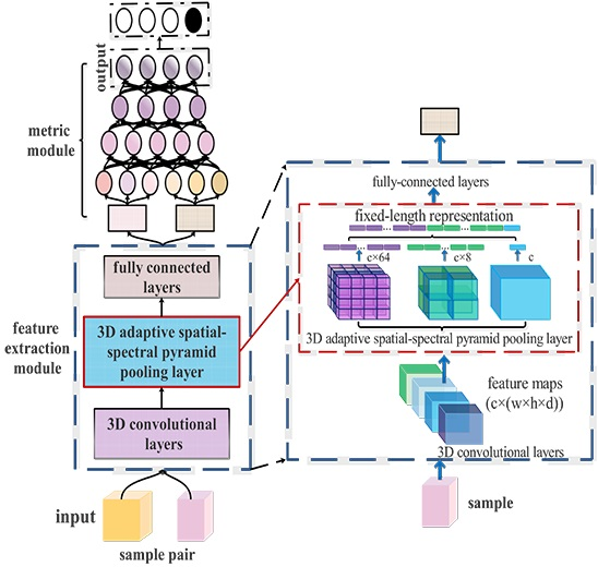
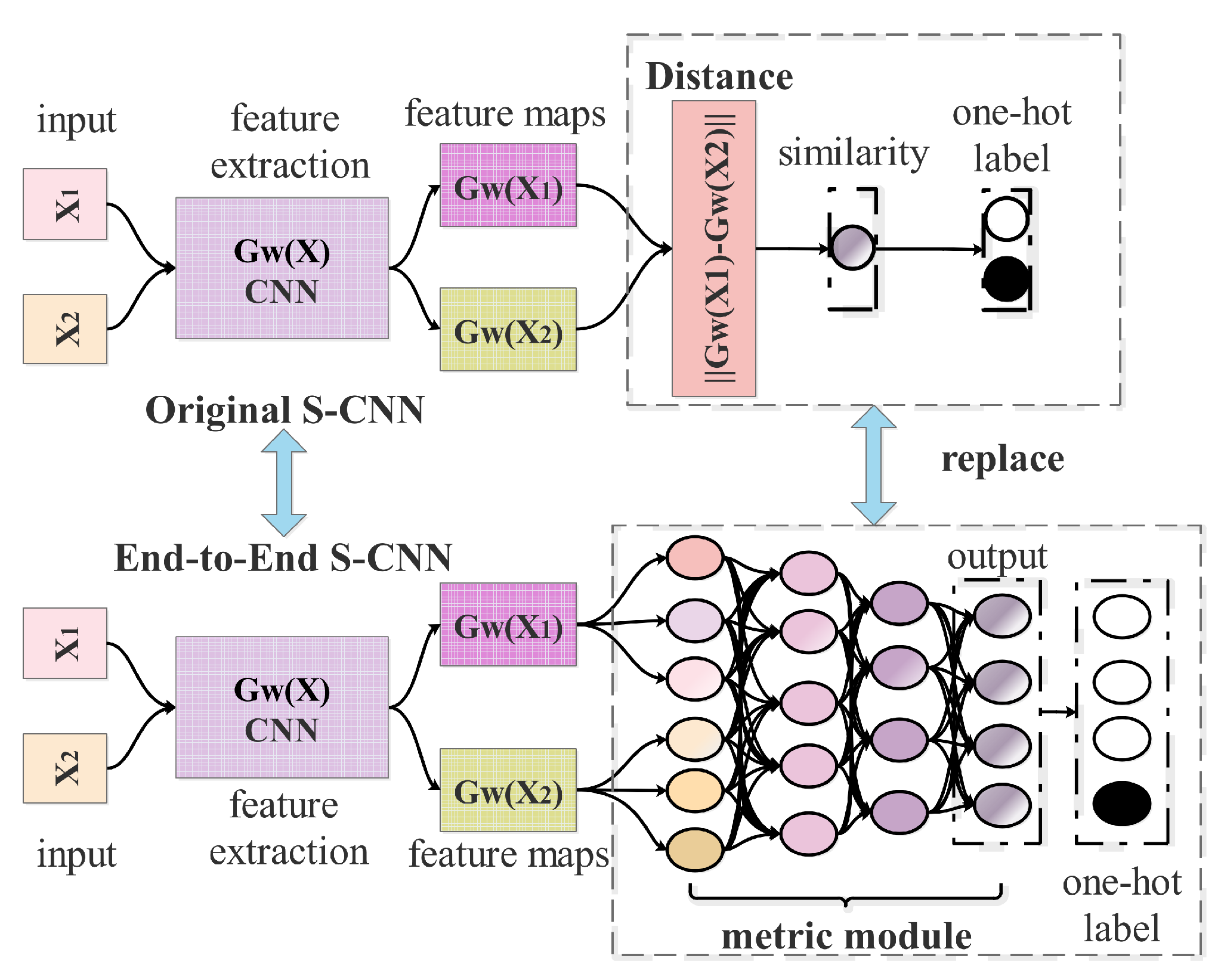
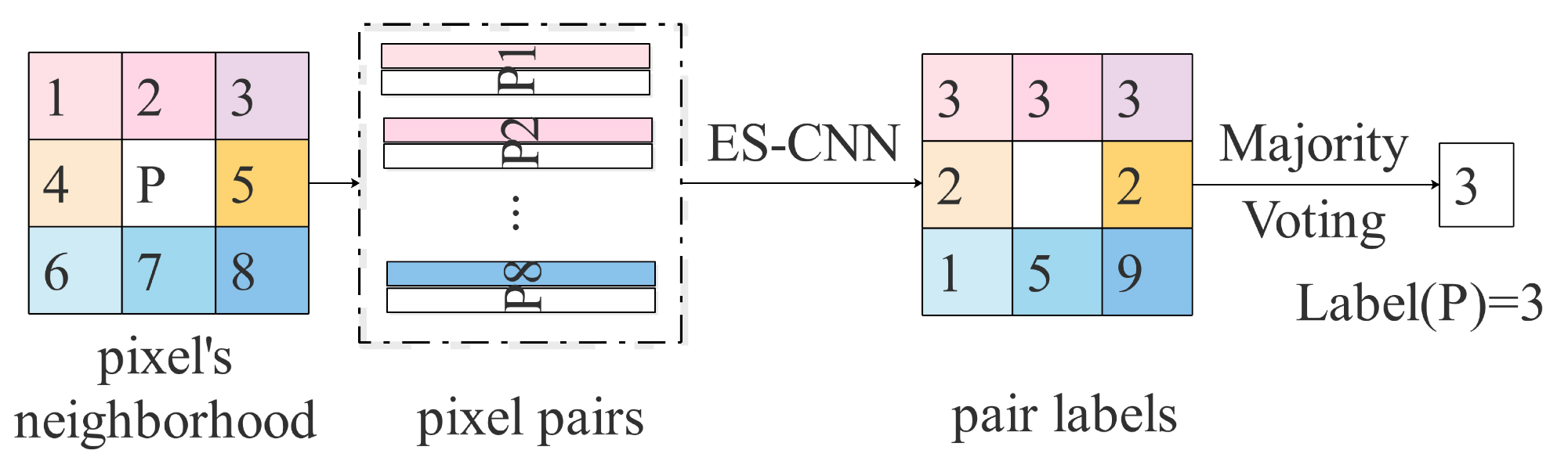
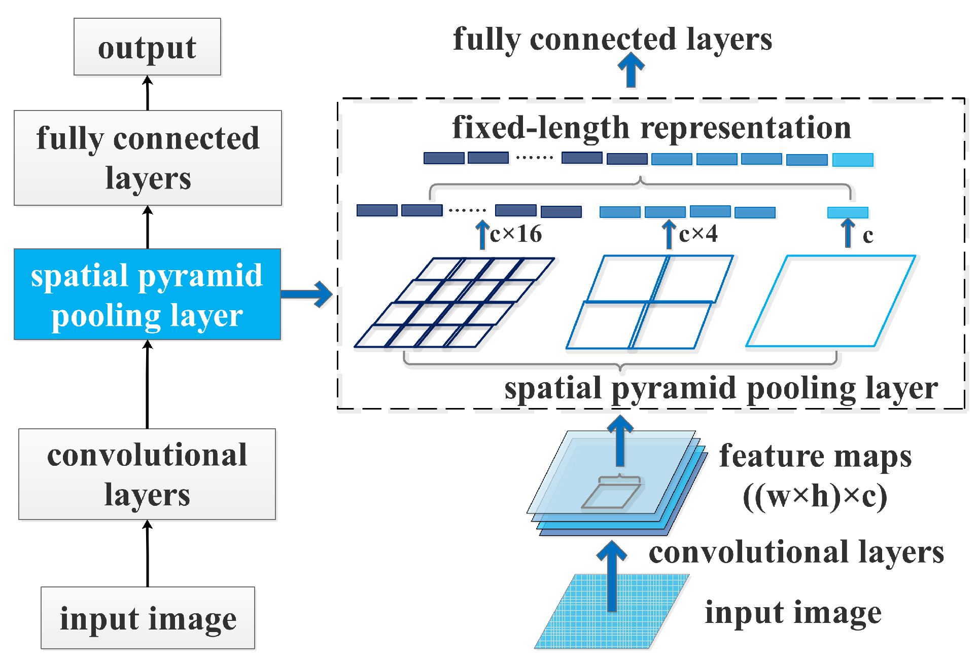
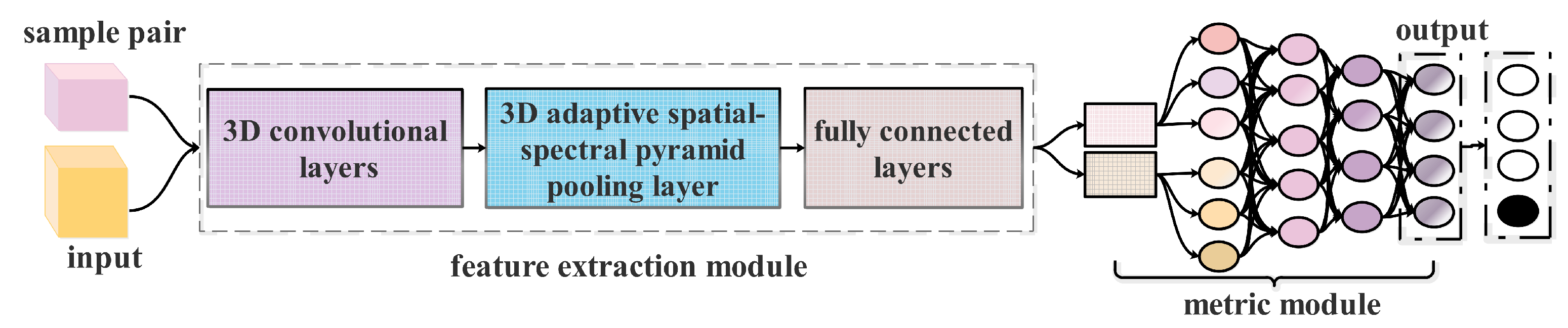
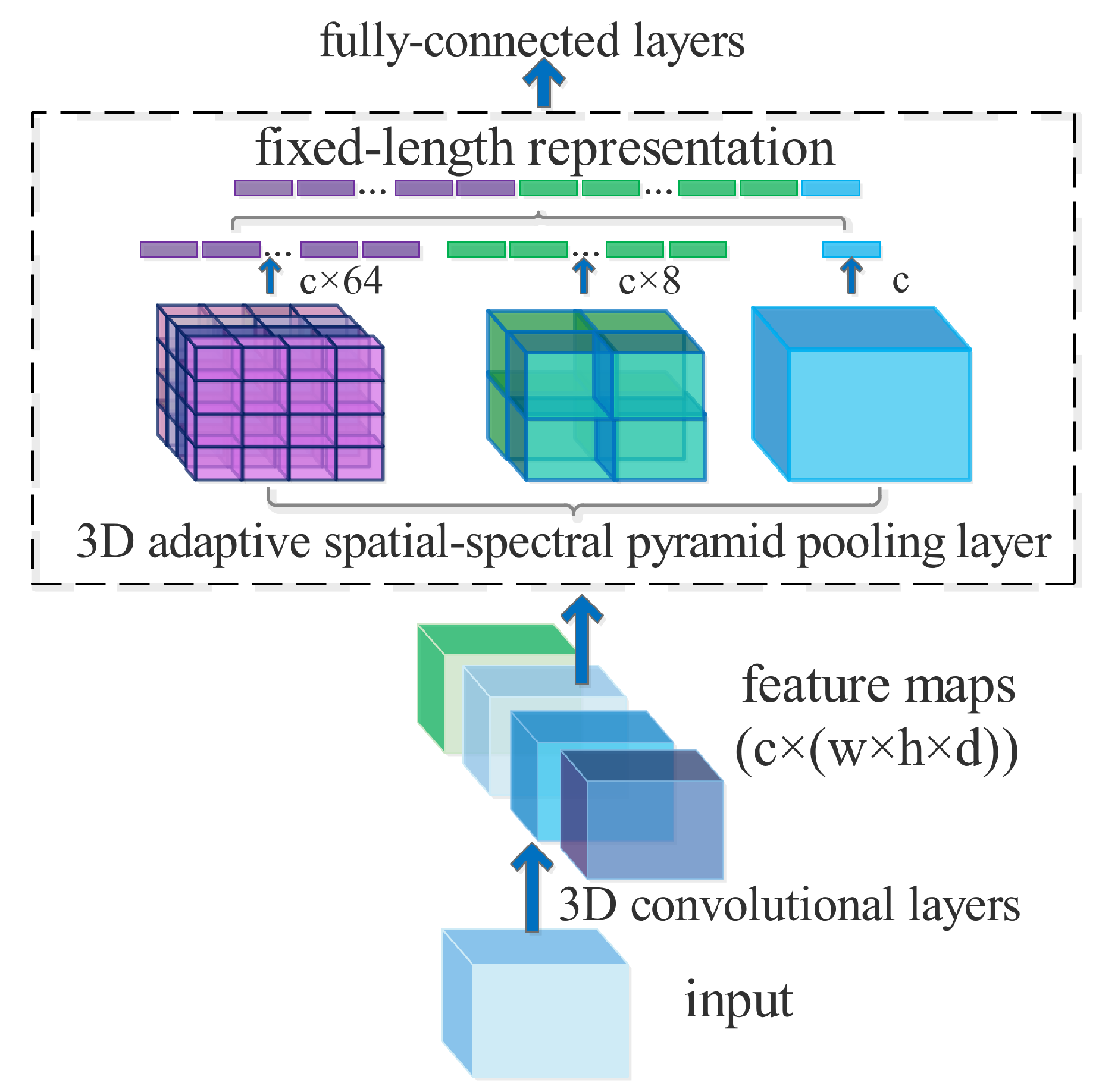
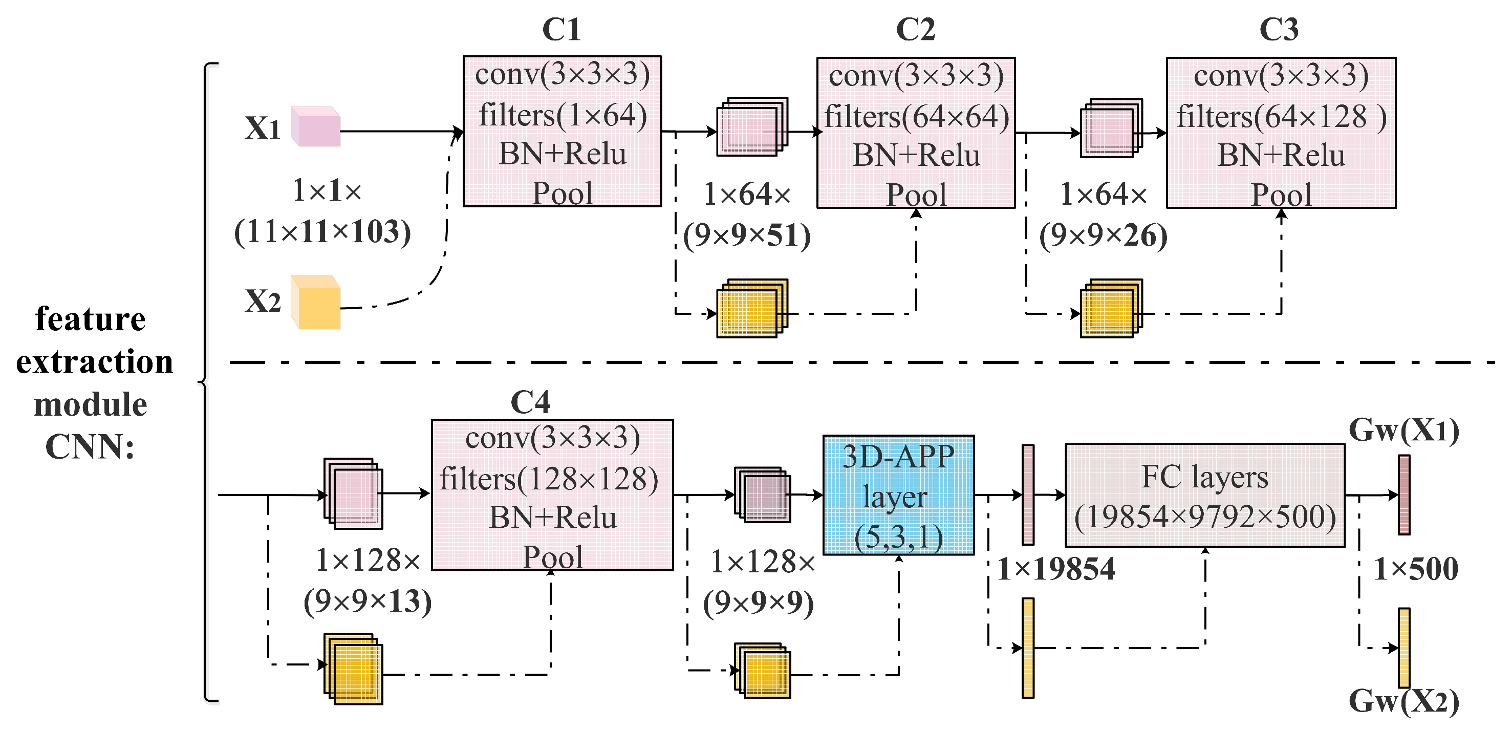
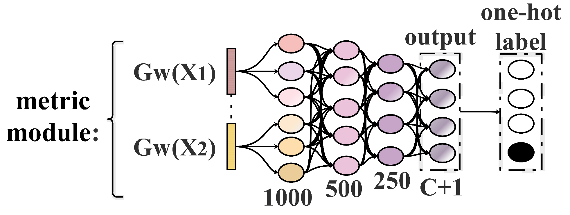
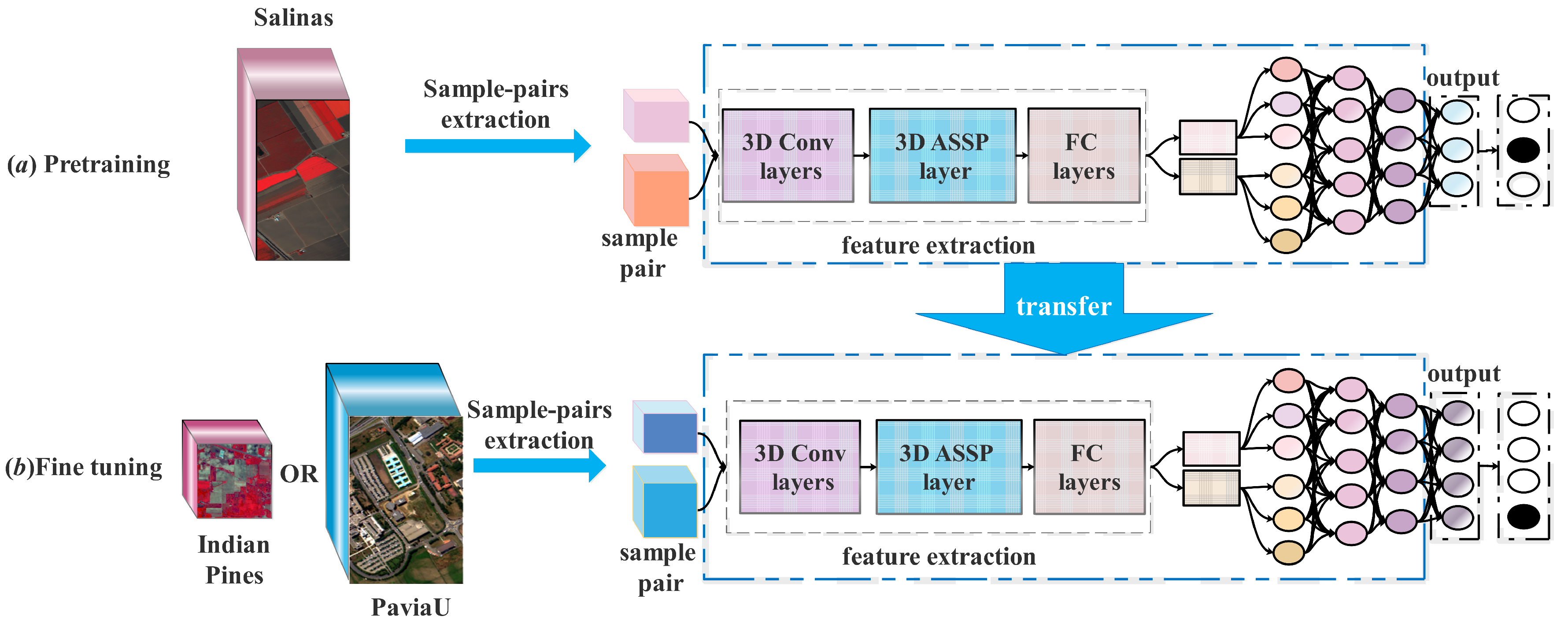
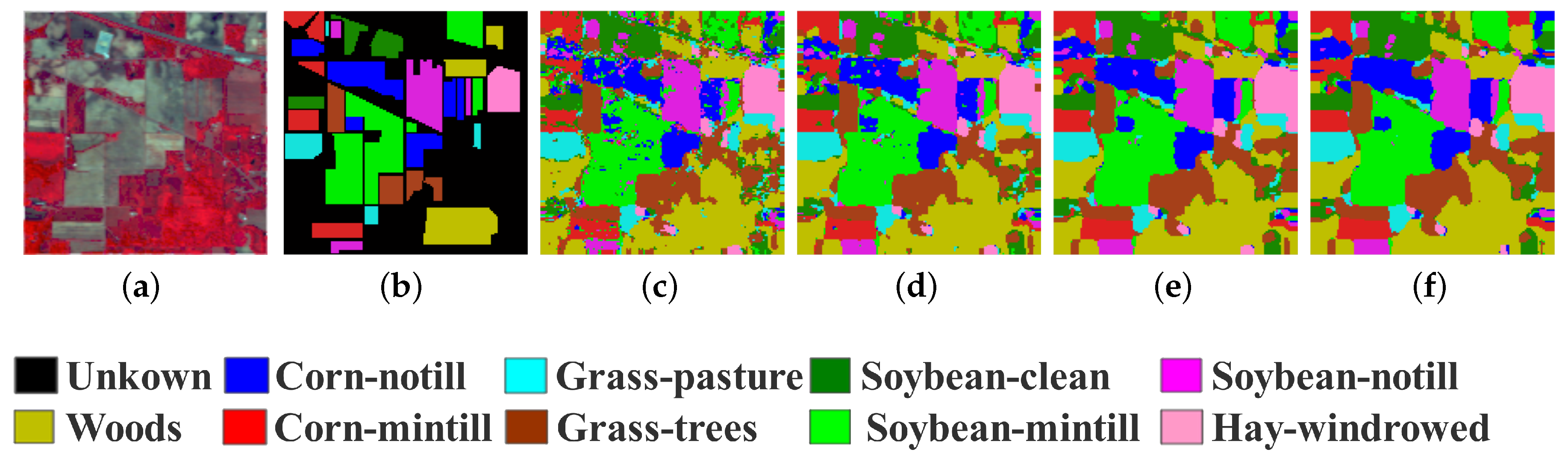
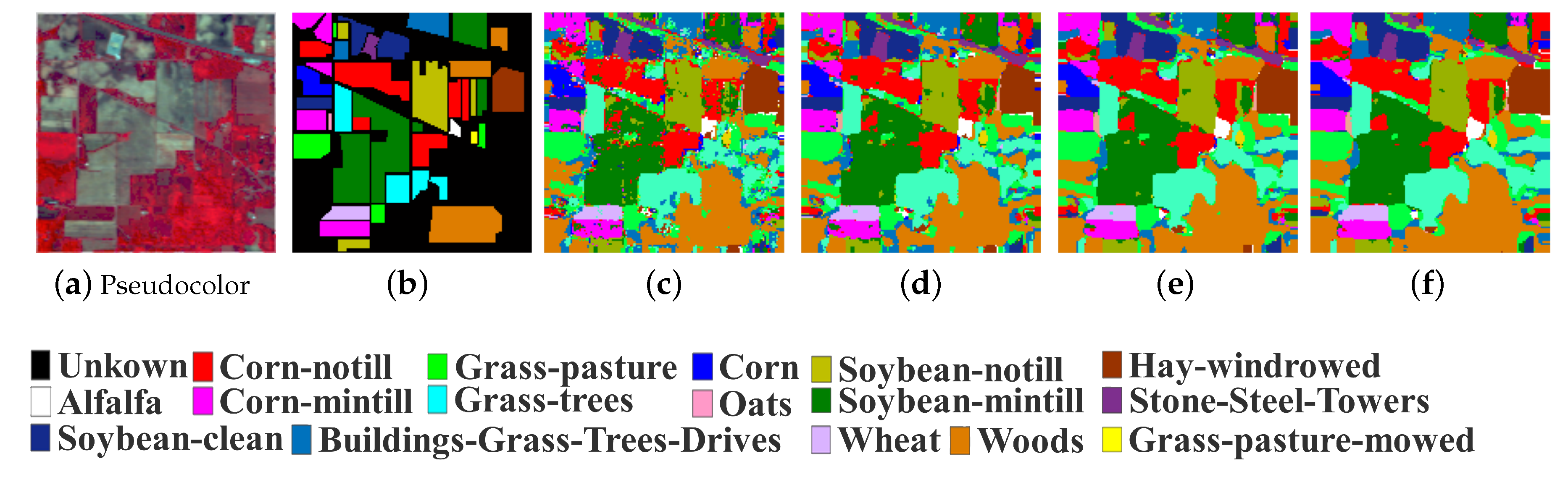
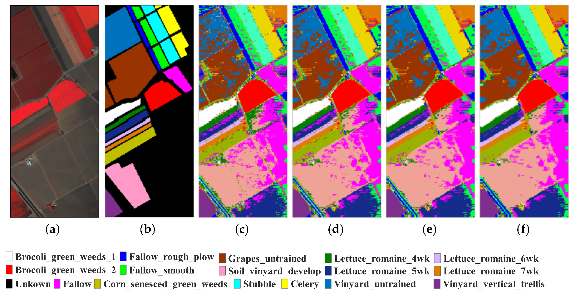
Table 1.
Details of the Three Data Sets: Indian Pines, PaviaU, and Salinas.
| Indian Pines | PaiaU | Salinas | |
|---|---|---|---|
| Spatial size (pixels) | |||
| Spectral range (nm) | 400–2500 | 430–860 | 400–2500 |
| Number of bands | 200 | 103 | 204 |
| GSD (m) | 20 | 1.3 | 3.7 |
| Sensor type | AVIRIS | ROSIS | AVIRIS |
| Areas | Indiana | Pavia | California |
| Number of classes | 16 | 9 | 16 |
| Provider | Purdue University | Prof. Paolo Gamba | Jet Propulsion Laboratory |
Table 2.
Statisticsof Training pixels, Validation pixels and Testing pixels for the Indian Pines DataSet.
Table 2.
Statisticsof Training pixels, Validation pixels and Testing pixels for the Indian Pines DataSet.
| No. | Class | Training | Validation | Testing |
|---|---|---|---|---|
| 1 | Alfalfa | 18 | 4 | 24 |
| 2 | Corn-notill | 180 | 20 | 1228 |
| 3 | Corn-mintill | 180 | 20 | 630 |
| 4 | Corn | 94 | 23 | 120 |
| 5 | Grass-pasture | 180 | 20 | 283 |
| 6 | Grass-trees | 180 | 20 | 530 |
| 7 | Grass-pasture-mowed | 11 | 2 | 15 |
| 8 | Hay-windrowed | 180 | 20 | 278 |
| 9 | Oats | 8 | 2 | 10 |
| 10 | Soybean-notill | 180 | 20 | 772 |
| 11 | Soybean-mintill | 180 | 20 | 2255 |
| 12 | Soybean-clean | 180 | 20 | 393 |
| 13 | Wheat | 82 | 20 | 103 |
| 14 | Woods | 180 | 20 | 1065 |
| 15 | Building-Grass-Trees-Drives | 154 | 38 | 194 |
| 16 | Stone-Steel-Towers | 37 | 9 | 47 |
| Tota | 2024 | 278 | 7947 | |
Table 3.
Statistics of Training pixels, Validation pixels and Testing pixels for the PaviaU DataSet.
Table 3.
Statistics of Training pixels, Validation pixels and Testing pixels for the PaviaU DataSet.
| No. | Class | Training | Validation | Testing |
|---|---|---|---|---|
| 1 | Asphalt | 180 | 20 | 6431 |
| 2 | Meadows | 180 | 20 | 18,449 |
| 3 | Gravel | 180 | 20 | 1899 |
| 4 | Trees | 180 | 20 | 2864 |
| 5 | Sheets | 180 | 20 | 1145 |
| 6 | Bare Soil | 180 | 20 | 4829 |
| 7 | Bitumen | 180 | 20 | 1130 |
| 8 | Bricks | 180 | 20 | 3482 |
| 9 | Shadows | 180 | 20 | 747 |
| Total | 1620 | 180 | 40,976 | |
Table 4.
Statistics of Training pixels, Validation pixels and Testing pixels for the Salinas DataSet.
Table 4.
Statistics of Training pixels, Validation pixels and Testing pixels for the Salinas DataSet.
| No. | Class | Training | Validation | Testing |
|---|---|---|---|---|
| 1 | Broccoli_green_weeds_1 | 180 | 20 | 1809 |
| 2 | Broccoli_green_weeds_2 | 180 | 20 | 3526 |
| 3 | Fallow | 180 | 20 | 1776 |
| 4 | Fallow_rough_plow | 180 | 20 | 1194 |
| 5 | Fallow_smooth | 180 | 20 | 2478 |
| 6 | Stubble | 180 | 20 | 3759 |
| 7 | Celery | 180 | 20 | 3379 |
| 8 | Grapes_untrained | 180 | 20 | 11,071 |
| 9 | Soil_vineyard_develop | 180 | 20 | 6003 |
| 10 | Corn_senesced_green_weeds | 180 | 20 | 3078 |
| 11 | Lettuce_romaine_4wk | 180 | 20 | 868 |
| 12 | Lettuce_romaine_5wk | 180 | 20 | 1727 |
| 13 | Lettuce_romaine_6wk | 180 | 20 | 716 |
| 14 | Lettuce_romaine_7wk | 180 | 20 | 870 |
| 15 | Vineyard_untrained | 180 | 20 | 7068 |
| 16 | Vineyard_vertical_trellis | 180 | 20 | 1607 |
| Total | 2880 | 320 | 50,929 | |
Table 5.
The sizes of training sample-pair set, validation sample-pair set and testing sample-pair set for The Three Data Sets: Indian Pines, PaviaU and Salinas. Here the number of spatial window K set to be 4 and the corresponding spatial window size are , , and .
Table 5.
The sizes of training sample-pair set, validation sample-pair set and testing sample-pair set for The Three Data Sets: Indian Pines, PaviaU and Salinas. Here the number of spatial window K set to be 4 and the corresponding spatial window size are , , and .
| Training Set | Validation Set | Testing Set | |
|---|---|---|---|
| Indian Pines | 16,386,304 | 278 | 7947 |
| PaviaU | 10,497,600 | 180 | 40,976 |
| Salinas | 33,177,600 | 320 | 50,929 |
Table 6.
Class-specific accuracy (%), OA (%) and Kappa coefficient generate by the ASSP-SCNNs on PaviaU dataset. Here we equip ASSP-SCNN with seven different ASSP layer with size and , respectively.
Table 6.
Class-specific accuracy (%), OA (%) and Kappa coefficient generate by the ASSP-SCNNs on PaviaU dataset. Here we equip ASSP-SCNN with seven different ASSP layer with size and , respectively.
| No. | |||||||
|---|---|---|---|---|---|---|---|
| 1 | 98.63 | 97.30 | 97.95 | 95.48 | 97.13 | 97.67 | 99.02 |
| 2 | 98.95 | 99.51 | 99.37 | 99.61 | 99.76 | 99.77 | 99.84 |
| 3 | 93.79 | 97.49 | 96.56 | 92.84 | 96.19 | 94.88 | 95.05 |
| 4 | 96.05 | 97.10 | 97.15 | 97.61 | 98.89 | 98.69 | 98.86 |
| 5 | 97.65 | 99.96 | 99.83 | 99.18 | 99.26 | 99.13 | 99.96 |
| 6 | 97.12 | 99.01 | 99.53 | 99.32 | 99.41 | 98.92 | 99.49 |
| 7 | 93.56 | 89.84 | 91.30 | 83.75 | 89.93 | 90.60 | 98.11 |
| 8 | 97.50 | 97.30 | 98.03 | 95.37 | 98.21 | 95.50 | 96.66 |
| 9 | 98.53 | 95.10 | 97.26 | 95.09 | 96.88 | 98.16 | 99.14 |
| OA | 97.906 | 98.289 | 98.504 | 97.511 | 98.582 | 98.358 | 99.048 |
| Kappa | 0.972 | 0.977 | 0.980 | 0.967 | 0.981 | 0.978 | 0.987 |
Table 7.
Class-specific accuracies (%), OA (%) and Kappa coefficients generate by the ASSP-SCNNs on PaviaU dataset. Here we train the ASSP-SCNN by a constructing 3D sample-pair set according to different spatial window size combinations and , respectively.
Table 7.
Class-specific accuracies (%), OA (%) and Kappa coefficients generate by the ASSP-SCNNs on PaviaU dataset. Here we train the ASSP-SCNN by a constructing 3D sample-pair set according to different spatial window size combinations and , respectively.
| No. | 7 | 9 | 11 | 13 | 15 | |||
|---|---|---|---|---|---|---|---|---|
| 1 | 97.95 | 98.00 | 99.02 | 98.31 | 98.03 | 99.34 | 99.60 | 99.10 |
| 2 | 98.90 | 99.31 | 99.84 | 99.46 | 99.18 | 99.43 | 99.69 | 99.87 |
| 3 | 95.62 | 96.49 | 95.05 | 97.49 | 96.53 | 98.76 | 97.75 | 99.55 |
| 4 | 95.29 | 99.18 | 98.86 | 96.84 | 95.65 | 97.58 | 98.52 | 99.39 |
| 5 | 99.83 | 99.44 | 99.96 | 99.39 | 98.54 | 99.96 | 99.83 | 100.00 |
| 6 | 98.09 | 97.63 | 99.49 | 98.96 | 99.09 | 98.68 | 99.23 | 99.47 |
| 7 | 94.96 | 93.43 | 98.11 | 96.98 | 96.76 | 97.47 | 98.81 | 97.39 |
| 8 | 96.17 | 97.18 | 96.66 | 97.55 | 98.06 | 98.91 | 98.48 | 99.51 |
| 9 | 94.62 | 94.44 | 99.14 | 93.55 | 95.46 | 97.84 | 96.70 | 97.45 |
| OA | 97.840 | 98.323 | 99.048 | 98.592 | 98.358 | 99.051 | 99.268 | 99.512 |
| Kappa | 0.971 | 0.978 | 0.987 | 0.981 | 0.978 | 0.987 | 0.990 | 0.993 |
Table 8.
Class-specific accuracy (%), OA (%) and Kappa coefficient of ASSP-SCNN and the comparing methods on Indian Pines dataset with nine classes.
Table 8.
Class-specific accuracy (%), OA (%) and Kappa coefficient of ASSP-SCNN and the comparing methods on Indian Pines dataset with nine classes.
| No. | SVM-RFS | 1D-CNN | CNN-PPF | C-CNN | SVM+SCNN | DFSL+SVM | ASSP-SCNN |
|---|---|---|---|---|---|---|---|
| 2 | 88.73 | 79.63 | 92.99 | 96.28 | 98.25 | 98.32 | 99.27 |
| 3 | 91.20 | 69.48 | 96.66 | 92.26 | 99.64 | 99.76 | 98.44 |
| 5 | 97.52 | 85.80 | 98.58 | 99.30 | 97.10 | 100.00 | 99.65 |
| 6 | 99.86 | 94.95 | 100.00 | 99.25 | 99.86 | 100.00 | 99.72 |
| 8 | 100.00 | 98.57 | 100.00 | 100.00 | 100.00 | 100.00 | 100.00 |
| 10 | 91.67 | 71.41 | 96.24 | 92.84 | 98.87 | 97.84 | 99.29 |
| 11 | 78.79 | 90.44 | 87.80 | 98.21 | 98.57 | 95.93 | 98.77 |
| 12 | 93.76 | 72.26 | 98.98 | 92.45 | 100.00 | 99.66 | 98.62 |
| 14 | 98.74 | 99.90 | 99.81 | 98.98 | 100.00 | 99.76 | 99.81 |
| OA | 89.83 | 84.44 | 94.34 | 96.76 | 99.04 | 98.35 | 99.17 |
| Kappa | 0.871 | 0.825 | 0.947 | 0.959 | 0.989 | 0.981 | 0.990 |
Table 9.
Class-specific accuracy (%), OA (%) and Kappa coefficient of ASSP-SCNN and the comparing methods on PaviaU dataset with nine classes.
Table 9.
Class-specific accuracy (%), OA (%) and Kappa coefficient of ASSP-SCNN and the comparing methods on PaviaU dataset with nine classes.
| No. | SVM-RFS | dgcForest | 1D-CNN | CNN-PPF | C-CNN | SVM+SCNN | DFSL+SVM | ASSP-SCNN |
|---|---|---|---|---|---|---|---|---|
| 1 | 87.95 | 92.92 | 85.62 | 97.42 | 97.40 | 98.69 | 97.18 | 99.13 |
| 2 | 97.17 | 96.88 | 88.92 | 95.76 | 99.40 | 99.58 | 99.40 | 99.95 |
| 3 | 86.99 | 74.31 | 80.51 | 94.52 | 94.48 | 99.52 | 97.90 | 98.44 |
| 4 | 95.50 | 90.79 | 96.93 | 97.52 | 99.16 | 99.22 | 98.40 | 99.46 |
| 5 | 99.85 | 98.90 | 99.30 | 100.00 | 100.00 | 100.00 | 100.00 | 99.83 |
| 6 | 94.31 | 78.60 | 84.30 | 99.13 | 98.70 | 98.85 | 99.56 | 99.91 |
| 7 | 94.74 | 78.76 | 92.39 | 96.19 | 100.00 | 99.32 | 99.25 | 96.87 |
| 8 | 85.89 | 87.69 | 80.73 | 93.62 | 94.57 | 96.58 | 95.52 | 98.87 |
| 9 | 99.89 | 99.85 | 99.20 | 99.87 | 99.87 | 100.00 | 99.68 | 99.34 |
| OA | 91.10 | 91.35 | 87.90 | 96.48 | 98.41 | 99.08 | 98.62 | 99.52 |
| Kappa | 0.882 | 0.884 | 0.838 | 0.951 | 0.979 | 0.988 | 0.982 | 0.993 |
Table 10.
Class-specific accuracy (%), OA (%) and Kappa coefficient of ASSP-SCNN and the comparing methods on Salinas dataset with sixteen classes.
Table 10.
Class-specific accuracy (%), OA (%) and Kappa coefficient of ASSP-SCNN and the comparing methods on Salinas dataset with sixteen classes.
| No. | SVM-RFS | dgcForest | 1D-CNN | CNN-PPF | C-CNN | DFSL+SVM | ASSP-SCNN |
|---|---|---|---|---|---|---|---|
| 1 | 99.55 | 99.48 | 98.73 | 100.00 | 100.00 | 100.00 | 99.97 |
| 2 | 99.92 | 99.81 | 99.12 | .88 | 99.89 | 99.97 | 99.99 |
| 3 | 99.44 | 99.10 | 96.08 | 99.60 | 99.89 | 100.00 | 99.97 |
| 4 | 99.86 | 99.38 | 99.71 | 99.49 | 99.25 | 99.86 | 99.83 |
| 5 | 98.02 | 97.92 | 97.04 | 98.34 | 99.39 | 100.00 | 99.94 |
| 6 | 99.70 | 99.74 | 99.59 | 99.97 | 100.00 | 100.00 | 99.99 |
| 7 | 99.69 | 99.32 | 99.33 | 100.00 | 99.82 | 100.00 | 99.84 |
| 8 | 84.85 | 87.71 | 78.64 | 88.68 | 91.45 | 91.67 | 95.95 |
| 9 | 99.58 | 99.42 | 98.04 | 98.33 | 99.95 | 99.69 | 99.99 |
| 10 | 96.49 | 93.20 | 92.38 | 98.60 | 98.51 | 99.79 | 98.90 |
| 11 | 98.78 | 96.06 | 99.14 | 99.54 | 99.31 | 100.00 | 98.52 |
| 12 | 100.00 | 99.30 | 99.88 | 100.00 | 100.00 | 100.00 | 99.94 |
| 13 | 99.13 | 98.22 | 97.84 | 99.44 | 99.72 | 100.00 | 99.86 |
| 14 | 98.97 | 92.40 | 96.17 | 98.96 | 100.00 | 100.00 | 98.36 |
| 15 | 76.38 | 68.05 | 72.69 | 83.53 | 96.24 | 97.01 | 94.16 |
| 16 | 99.56 | 97.80 | 98.59 | 99.31 | 99.63 | 99.94 | 99.44 |
| OA | 93.15 | 92.07 | 90.25 | 94.80 | 97.42 | 97.81 | 98.15 |
| Kappa | 0.923 | 0.912 | 0.895 | 0.938 | 0.971 | 0.976 | 0.979 |
Table 11.
Class-specific accuracy (%), OA (%) and Kappa coefficient of ASSP-SCNN on Indian Pines dataset with sixteen classes.
Table 11.
Class-specific accuracy (%), OA (%) and Kappa coefficient of ASSP-SCNN on Indian Pines dataset with sixteen classes.
| Class No. | Training Number | Class-Specific Accuracy | Class No. | Training Number | Class-Specific Accuracy |
|---|---|---|---|---|---|
| 1 | 18 | 97.96 | 9 | 8 | 90.91 |
| 2 | 180 | 95.88 | 10 | 180 | 96.56 |
| 3 | 180 | 98.50 | 11 | 180 | 97.31 |
| 4 | 94 | 98.74 | 12 | 180 | 596.54 |
| 5 | 180 | 99.82 | 13 | 82 | 100.00 |
| 6 | 180 | 99.91 | 14 | 180 | 99.76 |
| 7 | 11 | 100.00 | 15 | 154 | 98.48 |
| 8 | 180 | 100.00 | 16 | 37 | 98.95 |
| OA | 97.848 | Kappa | 0.975 | ||
Table 12.
OA (%) generated by the ASSP-SCNN-based transfer learning framework between the three HSI datasets.
Table 12.
OA (%) generated by the ASSP-SCNN-based transfer learning framework between the three HSI datasets.
| Source Dataset | Number of Labeled Pixels per Class for Fine-Tuning | Target Dataset | ||||
|---|---|---|---|---|---|---|
| 25 | 50 | 100 | 150 | 200 | ||
| Indian Pines_9 | 93.648 | 97.138 | 98.055 | 98.788 | 99.132 | Indian Pines_16 |
| 93.925 | 96.458 | 99.011 | 99.237 | 99.549 | PaviaU | |
| 92.900 | 93.865 | 96.512 | 97.470 | 97.997 | Salinas | |
| Indian Pines_16 | 98.213 | 98.156 | 97.840 | 99.137 | 99.475 | Indian Pines_9 |
| 92.247 | 96.156 | 98.543 | 99.353 | 99.614 | PaviaU | |
| 92.849 | 94.408 | 96.754 | 97.854 | 98.315 | Salinas | |
| PaviaU | 83.716 | 94.410 | 96.460 | 98.034 | 98.803 | Indian Pines_9 |
| 79.397 | 89.128 | 95.733 | 97.353 | 98.425 | Indian Pines_16 | |
| 92.682 | 93.833 | 96.954 | 97.823 | 98.209 | Salinas | |
| Salinas | 83.494 | 91.337 | 96.472 | 98.300 | 98.709 | Indian Pines_9 |
| 73.015 | 88.345 | 95.199 | 97.423 | 98.226 | Indian Pines_16 | |
| 93.833 | 95.289 | 98.450 | 99.331 | 99.492 | PaviaU | |
Table 13.
Time (hour) for training ASSP-SCNN without pre-training or fine-tuning the pre-trained ASSP-SCNN on three HSI target datasets.
Table 13.
Time (hour) for training ASSP-SCNN without pre-training or fine-tuning the pre-trained ASSP-SCNN on three HSI target datasets.
| Target Dataset | Without | Pre-Training on | Pre-Training on | Pre-Training on | Pre-Training on |
|---|---|---|---|---|---|
| Pre-Training | Indian Pines_9 | Indian Pines_16 | PaviaU | Salinas | |
| Indian Pines_9 (>98.6%) | 2.7 | / | 0.4 | 3.3 | 6.9 |
| Indian Pines_16 (>97.5%) | 9.5 | 0.4 | / | 8.0 | 10.7 |
| PaviaU (>99.4%) | 7.1 | 5.4 | 5.5 | / | 2.8 |
| Salinas (>97.9%) | 14.9 | 6.8 | 5.2 | 2.6 | / |
© 2020 by the authors. Licensee MDPI, Basel, Switzerland. This article is an open access article distributed under the terms and conditions of the Creative Commons Attribution (CC BY) license (http://creativecommons.org/licenses/by/4.0/).
Share and Cite
MDPI and ACS Style
Rao, M.; Tang, P.; Zhang, Z. A Developed Siamese CNN with 3D Adaptive Spatial-Spectral Pyramid Pooling for Hyperspectral Image Classification. Remote Sens. 2020, 12, 1964. https://0-doi-org.brum.beds.ac.uk/10.3390/rs12121964
AMA Style
Rao M, Tang P, Zhang Z. A Developed Siamese CNN with 3D Adaptive Spatial-Spectral Pyramid Pooling for Hyperspectral Image Classification. Remote Sensing. 2020; 12(12):1964. https://0-doi-org.brum.beds.ac.uk/10.3390/rs12121964
Chicago/Turabian StyleRao, Mengbin, Ping Tang, and Zheng Zhang. 2020. "A Developed Siamese CNN with 3D Adaptive Spatial-Spectral Pyramid Pooling for Hyperspectral Image Classification" Remote Sensing 12, no. 12: 1964. https://0-doi-org.brum.beds.ac.uk/10.3390/rs12121964
Note that from the first issue of 2016, this journal uses article numbers instead of page numbers. See further details here.