Sensitivity of Modeled CO₂ Air–Sea Flux in a Coastal Environment to Surface Temperature Gradients, Surfactants, and Satellite Data Assimilation

Abstract

This work evaluates the sensitivity of CO₂ air–sea gas exchange in a coastal site to four different model system configurations of the 1D coupled hydrodynamic–ecosystem model GOTM–ERSEM, towards identifying critical dynamics of relevance when specifically addressing quantification of air–sea CO₂ exchange. The European Sea Regional Ecosystem Model (ERSEM) is a biomass and functional group-based biogeochemical model that includes a comprehensive carbonate system and explicitly simulates the production of dissolved organic carbon, dissolved inorganic carbon and organic matter. The model was implemented at the coastal station L4 (4 nm south of Plymouth, 50°15.00’N, 4°13.02’W, depth of 51 m). The model performance was evaluated using more than 1500 hydrological and biochemical observations routinely collected at L4 through the Western Coastal Observatory activities of 2008–2009. In addition to a reference simulation (A), we ran three distinct experiments to investigate the sensitivity of the carbonate system and modeled air–sea fluxes to (B) the sea-surface temperature (SST) diurnal cycle and thus also the near-surface vertical gradients, (C) biological suppression of gas exchange and (D) data assimilation using satellite Earth observation data. The reference simulation captures well the physical environment (simulated SST has a correlation with observations equal to 0.94 with a p > 0.95). Overall, the model captures the seasonal signal in most biogeochemical variables including the air–sea flux of CO₂ and primary production and can capture some of the intra-seasonal variability and short-lived blooms. The model correctly reproduces the seasonality of nutrients (correlation > 0.80 for silicate, nitrate and phosphate), surface chlorophyll-a (correlation > 0.43) and total biomass (correlation > 0.7) in a two year run for 2008–2009. The model simulates well the concentration of DIC, pH and in-water partial pressure of CO₂ (pCO₂) with correlations between 0.4–0.5. The model result suggest that L4 is a weak net source of CO₂ (0.3–1.8 molCm⁻² year⁻¹). The results of the three sensitivity experiments indicate that both resolving the temperature profile near the surface and assimilation of surface chlorophyll-a significantly impact the skill of simulating the biogeochemistry at L4 and all of the carbonate chemistry related variables. These results indicate that our forecasting ability of CO₂ air–sea flux in shelf seas environments and their impact in climate modeling should consider both model refinements as means of reducing uncertainties and errors in any future climate projections.

1. Introduction

Recent research efforts in marine and climate disciplines highlight the effects that increasing atmospheric CO₂ concentrations are having on the Earth’s climate and in its control over the oceanic carbonate system and pH [1]. As one of the greenhouse gases, its air–sea flux is a critical part of the climate system.

Atmospheric carbon dioxide (CO₂) has been increasing since the industrial revolution due to the burning of fossil fuels, cement production and land use change. While it is generally accepted that the ocean system annually absorbs up to 30% of the CO₂ released by burning fossil fuels [2], it is not clear whether this ocean carbon ‘sink’ is increasing or decreasing, and considerable temporal and spatial inter-annual variation appears to occur [3]. The flux of CO₂ between the atmosphere and the ocean (air–sea) is primarily controlled by conditions of the physical environment like wind speed, sea state and sea-surface temperature but also by biological processes taking place in the euphotic zone. Adding CO₂ to seawater disrupts the carbonate system, leading to an increase in free CO₂/carbonic acid and the bicarbonate ion concentration while decreasing the carbonate ion, pH and carbonate saturation states [4]. All of these have implications for a range of biological and chemical processes like calcification, primary production and reproduction [5,6].

In shelf seas, CO₂ dynamics are highly variable in space and time [7,8] partly driven by the high primary productivity, leading to a large draw-down of dissolved inorganic carbon (DIC, the sum of CO₂, bicarbonate and carbonate ions) and consequent rise in pH [9]. This is further complicated by the close link between benthic processes and the pelagic carbon cycle and alkalinity [10] and riverine inputs of DIC and total alkalinity (TA) into coastal systems [11].

In addition to these processes, diapycnal mixing across the thermocline drives a continuous change in surface CO₂ as a result of vertical fluxes of DIC and nutrients that stimulate primary production [12]. The existence of near-surface temperature variations was identified by Ward et al. [13] and their significance for air–sea CO₂ fluxes has been recently highlighted by Woolf et al. [14].

Clearly, further understanding the CO₂ pathways, sources, sinks, their respective budgets and their impacts on Earth’s climate system is essential for monitoring and projecting future climate scenarios.

In this work we evaluate the sensitivity of model derived CO₂ fluxes to physical and biological drivers in a shallow shelf sea location (L4) using the GOTM–ERSEM model [15]. The use of a 1D model here is appropriate because in shallow shelf seas, the vertical mixing is mainly driven by the balance between tidal mixing and atmospheric fluxes, especially solar heating.

L4 (4 nm south of Plymouth, 50°15.00′N, 4°13.02′W, depth of 51 m) is a coastal station in the western English Channel where sustained observations have been carried out since the late 1980s and where variability in planktonic communities has been described extensively [16]. In recent years, physical observations have intensified in the framework of the Western Channel Observatory [17] run by the Plymouth Marine Laboratory (PML) in cooperation with the Marine Biological Association (MBA). The environmental and water conditions at L4 have been sampled weekly and physico–chemical and biological observations are freely available. Recently, a mid-ocean buoy has been installed at L4 [18]. As in other shelf seas, physics at L4 are mainly the result of a balance between tidal mixing and atmospheric forcing and a seasonal temperature stratification appears when summer heating overcomes the tidal induced mixing. Nutrient dynamics and ecosystem dynamics are strongly dependent on this variability [17]. There are numerous reports of strong intra-seasonal and inter-annual variability in the plankton production and community composition in the western English Channel and in other shelf seas e.g., [16,19,20], all of which help to modulate and alter the air–sea flux of CO₂. Collectively, these data provide a substantial dataset to parameterize and evaluate the performance of coupled hydrodynamic–ecosystem models.

2. Methods

In this work we evaluate the sensitivity of modeled CO₂ fluxes to three methodological approaches which can affect the simulation of the carbonate system within ecosystem models. In doing so, we have defined three numerical experiments and one reference simulation that constitutes our baseline data to compare the changes associated with each experiment.

2.1. Physics Model Description: Gotm

The General Ocean Turbulence Model, (GOTM [21]) is a 1D physical model that is designed as a generic system for marine modeling. GOTM dynamically simulates the evolution of temperature, density and vertical mixing when forced with meteorological data (e.g., [15]). From all the turbulence model options available within GOTM we have chosen the second order turbulence model $\kappa$–$ϵ$ with the coefficients suggested in Canuto et al. [22] (version A) as Umlauf and Burchard [23] demonstrated that it can simulate turbulence in stratified shear flows in a physically sound and numerically robust way.

The sensible and latent heat fluxes are calculated within GOTM using standard formulae [24]. The calculations for the latent and sensible heat are dependent upon the calculation of their coefficients, which are a function of air–sea temperature difference, wind speed and a stability criterion for the surface waters [25]. The long wave (back) radiation is calculated using the May formulation [26]. The surface stress is calculated from the wind stress. These formulae were chosen based on a sensitivity study of surface heat flux formulation on the model response [27].

The physical model supplies the temperature to the ecosystem process descriptions and determines the fluxes of ecosystem components between adjacent boxes and or layers. The coupling of ERSEM and GOTM is described in [28].

2.2. Biological Model Description: Ersem

ERSEM is a generic ecosystem model based on the “functional group approach” [29,30]; the biota in the ecosystem are divided into three functional types: primary producers, consumers, and decomposers, which are subdivided on the basis of trophic links and/or size. ERSEM can produce a range of dynamics and community structures with a consistent parameterization, when applied to a wide variety of physical scenarios. The consistent parameterization is only possible because of the range of process descriptions now included in the model.

The model is capable of accurately simulating the spatial pattern of ecological fluxes throughout the seasonal cycle and the main phytoplankton succession (cg. [28,31]). It includes representations of the benthic system, which are vital for the correct treatment of shelf seas. Both physiological (ingestion, respiration, excretion and egestion) and population (growth and mortality) processes are described by fluxes of carbon and nutrients between functional groups. The associated decoupled carbon and nutrient dynamics gives a far better approximation to how nutrient limitation acts on cells than fixed quota models [30]. It can simulate both the classical, large cell dynamics and the small cell microbial loop, thereby representing the continuum of trophic pathways. ERSEM standard pelagic compartments include four phytoplankton functional groups; picoplankton (0.2–2 μm), nanoflagellates (2–20 μm), dinoflagellates (20–200 μm) and diatoms (20–200 μm) three zooplankton groups; heterotrophic nanoflagellates (<20 μm), microzooplankton (20–200 μm) and mesozooplankton (>200 μm) and a bacteria loop. Fractionation of dissolved and particulate matter and instantaneous light are also key aspects of the current model version. A more in-depth description of the model can be found in Allen et al. [28]. The model has been extensively validated with respect to the carbon system [8], chl-a [32,33], and nutrients and biomass [34,35]. The full ERSEM model open source code and manual can be found at http://www.pml.ac.uk/Modelling/Models/ERSEM.

2.3. Observations

Both in situ and satellite derived biological measurements were used for model skill assessment and/or assimilation. These observations are described in the following sections.

2.3.1. In Situ Biological Measurements

The observations were obtained under the weekly sampling strategy of the Western Channel Observatory. The water samples were collected using Niskin bottles mounted on the CTD rosette frame. Surface nutrient measurements of silicate, phosphate, nitrate, nitrite and ammonium where measured colorimetrically using a Bran and Luebbe AAIII segmented flow autoanalyzer [36]. For chl-a measurements, 1 or 2 L of seawater from four depths (0, 10, 20 and 50 m) was filtered onto a Whatman^®GF/F glass microfiber filter and the filter stored in liquid nitrogen until analysis. For the analysis stage, pigments were extracted from the thawed GF/F filter into 2 mL methanol [37] and sonicated for 35 s. These extracts were then centrifuged to remove filter and cell debris (5 min at 4000 rpm) and analyzed using reversed-phase HPLC [38]. Pigments, including chl-a, were identified using retention time and spectrally matched using photo-diode array spectroscopy [39]. Water samples from 10 m depth were used for quantifying the phytoplankton and microzooplankton community composition and abundance from microscopic analysis of samples preserved with Lugol’s iodine. Cell were identified to species-level were possible and assigned to three functional groups (diatoms (centric and pennate), dinoflagellates and flagellates). The conversion from cell numbers to biomass was based on volumes according to geometric shapes and formulae of Olenina et al. [40] and Menden-Deuer and Lessard [41].

Photosynthesis–irradiance parameters (P–E) for the estimation of integrated primary production followed the methodology presented in Tilstone et al. [42] and Platt et al. [43]. The samples were incubated for 2–3 h after which the suspended material was filtered through 25 mm Whatman GF/F filters. The filters were exposed to concentrated HCl fumes for 12 h and radiocarbon activity on the filters was determined by a Packard Tri-Carb 2500 TR liquid scintillation analyzer using the external standard and the channel ratio methods to correct for quenching. The broadband P–E parameters were estimated by fitting the data to the model of Platt et al. [43]. The daily integrated productivity was estimated as in Tilstone et al. [42] at 1 m intervals from the sea surface down to 0.1% surface irradiance. Time series of in situ primary production at L4 is given in Barnes et al. [44].

The carbonate system was sampled at two depths; 2 m and bottom, using 250 mL glass bottles and preserved with 50 μL of saturated HgCl₂ solution. The samples were analyzed within 12 months by tritation (for total alkalinity) and coulometric analysis (for DIC). Full details of the analytical procedure and a thorough discussion of the carbonate system data can be found in Kitidis et al. [45].

2.3.2. Satellite Observations

Level 1a (calibrated and geolocated radiance) 1 km spatial resolution satellite remote sensing Earth observation (EO) data collected by the Moderate-Resolution Imaging Spectrometer (MODIS, onboard the Aqua platform) were downloaded from the NASA Ocean Color data distribution website (http://oceandata.sci.gsfc.nasa.gov/) for the 2009–2010 period. These were processed using the SeaWiFS Data Analysis System (SeaDAS, version 6.4) to generate 1 km chl-a data using the three-band algorithm, OC3 [46]. All products were quality masked using the default SeaDAS masks for land, cloud and high/saturated radiance [47].

2.4. Experiments

2.4.1. Experiment A

The reference simulation or Experiment A is described in Section 2.1 and Section 2.2. In this work, the GOTM model was configured with 50 vertical layers with a time step of 10 s. The vertical resolution is increased towards the bottom layer to better capture the dynamics of the bottom boundary layer. This results in a layer thickness of 30 cm at the bottom increasing logarithmically to 1.6 m from 15 m above the bottom to the surface.

For meteorological forcing, we use 6 hourly data from the National Center for Environmental Prediction/National Center for Atmospheric Research (NCEP/NCAR) reanalysis [48], which has a spatial resolution of 1.9° × 1.9°. The model is forced with air temperature, atmospheric pressure, 10 m winds and dew temperature. The shortwave radiation is imposed separately at 5 min intervals using locally observed values measured with a Li-Cor pyranometer (LI-200SZ) on a coastal station maintained by PML (http://www.westernchannelobservatory.org.uk/pml_weather_station).

Tidal forcing was included as time series of surface elevation gradients generated using 15 tidal harmonics extracted from the results of a high resolution (1.8 × 1.8 km grid spacing) 3D barotropic model simulation of the UK shelf [49]. The harmonics used are all the relevant semi-diurnal and diurnal tidal constituents such as M2, Q1, O1, P1, S1, K1, 2N₂, ${\mu }_2$, N2, u₂, L2, T2, S2, K2 and M4. Surface elevation gradients were obtained by artificially generating hourly surface elevation time series on adjacent grid points to the L4 station position using the t-tide MATLAB toolbox [50].

The model is initialized in winter when the water column is well-mixed with observed temperature and salinity profiles (see Section 2.3). The water column evolution is further constrained by nudging the model results to the observed temperature and salinity profiles with a relaxation time scale of two weeks [15,21]. In this way, GOTM can account for missing 3-dimensional dynamics not resolved within 1D models like the long-term horizontal advection of temperature and salinity that is important for resolving the vertical water column structure and hence gas fluxes in coastal regions [51]. An alternative approach to the introduction of water masses with different temperature and salinity signatures into the 1D water column is through the specification of time-varying, vertically resolved horizontal temperature and salinity gradients. This option is not employed here for this purpose due to the absence of such information, but the feature is used in Experiment D as a way to artificially introduce errors in the mixing dynamics as described in Section 2.4.4.2. The model is initialized where possible from observations taken in December 2005 (plankton biomass and nutrients) and run for two years until December 2007 to create a common start file for each of the experiments. The years 2006–2007 are taken as a model spin-up period and the model is evaluated against observations for the period 6 January 2008 until 20 December 2009. The model parameters used follow Blackford et al. [31] as modified by Artioli et al. [8].

2.4.2. Experiment B

Experiment B looks into the effects that resolving the diurnal SST cycle has on the air–sea fluxes of CO₂. By the diurnal cycle of SST we consider the changes of the temperature vertical structure in the top few meters of the ocean caused by the direct daytime solar heating and nighttime cooling. Therefore, to model these diurnal changes, the model resolution is increased logarithmically from 2 cm at the surface to 1 m at 10 m deep.

2.4.3. Experiment C

Experiment C evaluates the potential impacts that biologically generated surfactants have on air–sea fluxes. Sea-surface surfactants or organics can influence gas exchange in two ways, as a monolayer physical barrier and through modification of sea-surface hydrodynamics and hence turbulent energy transfer [52,53], manifesting as a reduced gas transfer velocity (K). For Experiment C, we have chosen to implement a primary productivity-based reduction on the gas transfer velocity. Several studies have tried to quantify this suppression of K (e.g., and references therein [53]). However, the exact magnitude and nature of the suppression is unclear as the values found among studies (in both the natural environment and within laboratories) vary considerably. So therefore we have chosen to investigate the sensitivity of the fluxes to this type of phenomenon rather than trying to quantify it.

2.4.4. Experiment D

The third Experiment (D) evaluates the impacts of using data assimilation of remotely sensed chlorophyll-a (chl-a) on the ability of ERSEM to simulate the carbonate system and its associated control on air–sea fluxes of CO₂.

2.4.4.1. The Ensemble Kalman filter (EnKF)

Experiment D evaluates the sensitivity of modeled CO₂ to data assimilation of surface chl-a as estimated from satellite. Following previous work we have chosen the Ensemble Kalman Filter [54] as implemented in the 1D GOTM–ERSEM model by Torres et al. [15] and used by [34] for this region. The Ensemble Kalman Filter method was formulated to work with non-linear models and in particular to handle the error covariance evolution [54]. Here the analysis scheme described in Evensen [55] is implemented. First the model is integrated forward in time with the addition of a stochastic term),

$${\mathsf{\Psi }}_{k+1}^f=\mathsf{f}\left({\mathsf{\Psi }}_k^a\right)+{\mathsf{q}}_k,$$

(1)

$\mathsf{q}$ representing the model errors and $\mathsf{f}$ represents a non-linear operator. $\mathsf{\Psi }$ is a matrix holding the model state variables. The k subscript indicates the time index, while the superscripts f and a correspond to the forecast and analysis. The model errors are represented through the covariances of the state variable errors. These are defined a priori and are evolved forward in time by the Kalman filter.

The information contained by a full probability density function can be represented by an ensemble of model states. Covariances can be defined with respect to a known true state or as expectations, ensemble covariance matrices around the ensemble mean, $\overline{\psi }$. Hence the ensemble of model states will provide information on statistical moments of interest.

$$\begin{array}{c}\hfill P^f\simeq \overline{({\psi }^f-\overline{{\psi }^f}){({\psi }^f-\overline{{\psi }^f})}^T}\end{array}$$

(2)

$$\begin{array}{c}\hfill P^a\simeq \overline{({\psi }^a-\overline{{\psi }_a}){({\psi }^a-\overline{{\psi }^a})}^T}.\end{array}$$

(3)

The standard EnKF analysis equation [56] is applied here. The analysis step involves updating each of the ensemble members taking into consideration the difference between the observations and the model state as well as the errors associated with the model state variables and the observations. As each ensemble is updated individually there is no need to regenerate them. The ensemble mean will be the updated state that minimizes the model variance. A more in-depth description of the algorithm can be found in Ciavatta et al. [34].

The variables included in the analysis are log transformed so that their variability is reduced, their Gaussianity is improved and positivity of the solution is guaranteed. The variables and the assimilated observations have been transformed by a Gaussian anamorphosis function natural log as suggested in Bertino et al. [57]. Other applications have been reported in Torres et al. [15], Ciavatta et al. [34], Nerger and Gregg [58].

Compared to the other model improvements from experiments B and C, the EnKF requires additional computing resources which scale with the number of ensembles required to correctly approximate the evolution of the probability density function of the model state. In our implementation, the setup required running 100 different model simulations and was therefore 100 times more computationally expensive than either Experiment B or C. For this reason, Experiment D focusses on a single year (2009).

2.4.4.2. Model Errors

The ensemble of model states defined in Equation (1) is obtained by adding model errors to the assimilation scheme. They are applied to all the pelagic variables included in the covariance matrix of state variables but not to the benthic state variables. The latter are not included in the analysis scheme and hence are not updated.

Two types of model errors are included in the simulations: those that modify the state variables and those that perturb the forcing functions. Errors assigned to most ERSEM state variables were 20% Gaussian error; they were reduced to 5% in the detritus related variables to limit large corrections to the largest pool in the model and in the nutrient variables as they constitute the best resolved variables in ERSEM. These errors are introduced once as initial conditions to generate the initial ensemble of model states, and at each analysis step before solving the Kalman filter equation.

Additional errors are introduced at run-time by perturbing the forcing functions that drive the primary production and the vertical transport of the biological state variables. At each time step of each ensemble simulation, errors are added to the surface irradiance values. Additional errors associated with the internal pressure gradients and background sediment concentration constant are randomly initialized and kept fixed during each assimilation cycle so that they are different for each ensemble member. The sea-surface irradiance and the background suspended sediment concentration are two forcing variables which have a large ecological importance as the light regime determines in great measure the short-term variability of phytoplankton. Both were assigned a 25% Gaussian error. The internal pressure gradients errors act to perturb the water column structure and consequently the vertical transport associated with mixing. The internal pressure gradients errors were calculated as pseudo-random fields as suggested by Evensen [56] with a correlation length equal to the total water depth (51 m).

2.4.4.3. Observational Errors

The Gaussian measurement errors of the MODIS derived surface chl-a were set to 30% for the months January to March and October to December when the EO chl-a retrievals are expected to be affected by high suspended sediments concentrations in the water and high solar zenith angle (Figure 1) [59]. Chl-a values were generally less than 1 mgCm⁻³ in those months. During the spring–summer period, EO errors were set at 10% to reflect the dominance of chl-a over the suspended sediment concentrations. We justify this by the good agreement found by Groom et al. [60] in comparing HPLC in situ chl-a with MODIS and SeaWiFS data who found no bias due to coastal adjacency in the ocean colour data at L4. They concluded that L4 could be considered case 2 waters in late autumn and winter and case 1 waters for the rest of the year.

3. Results

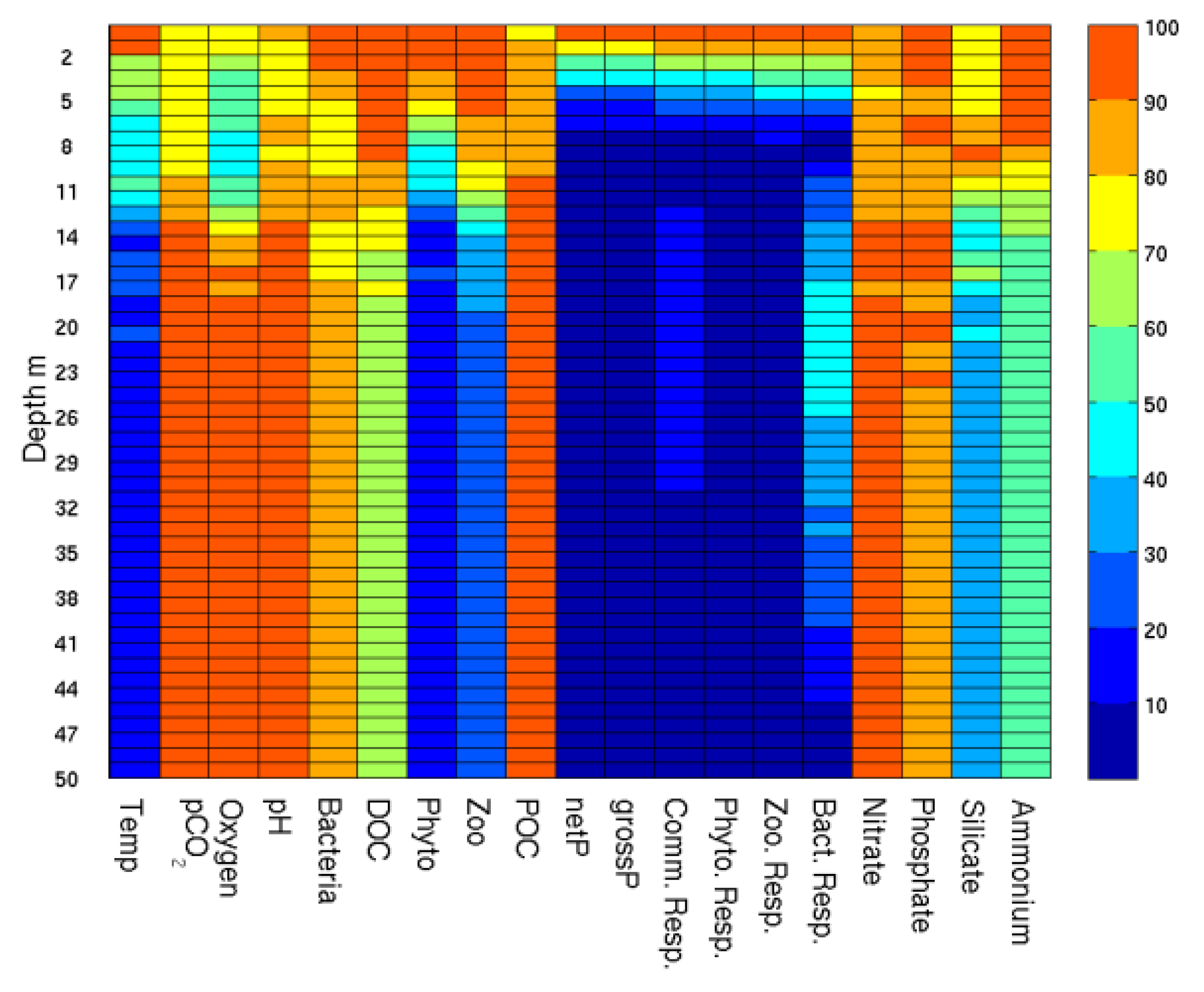
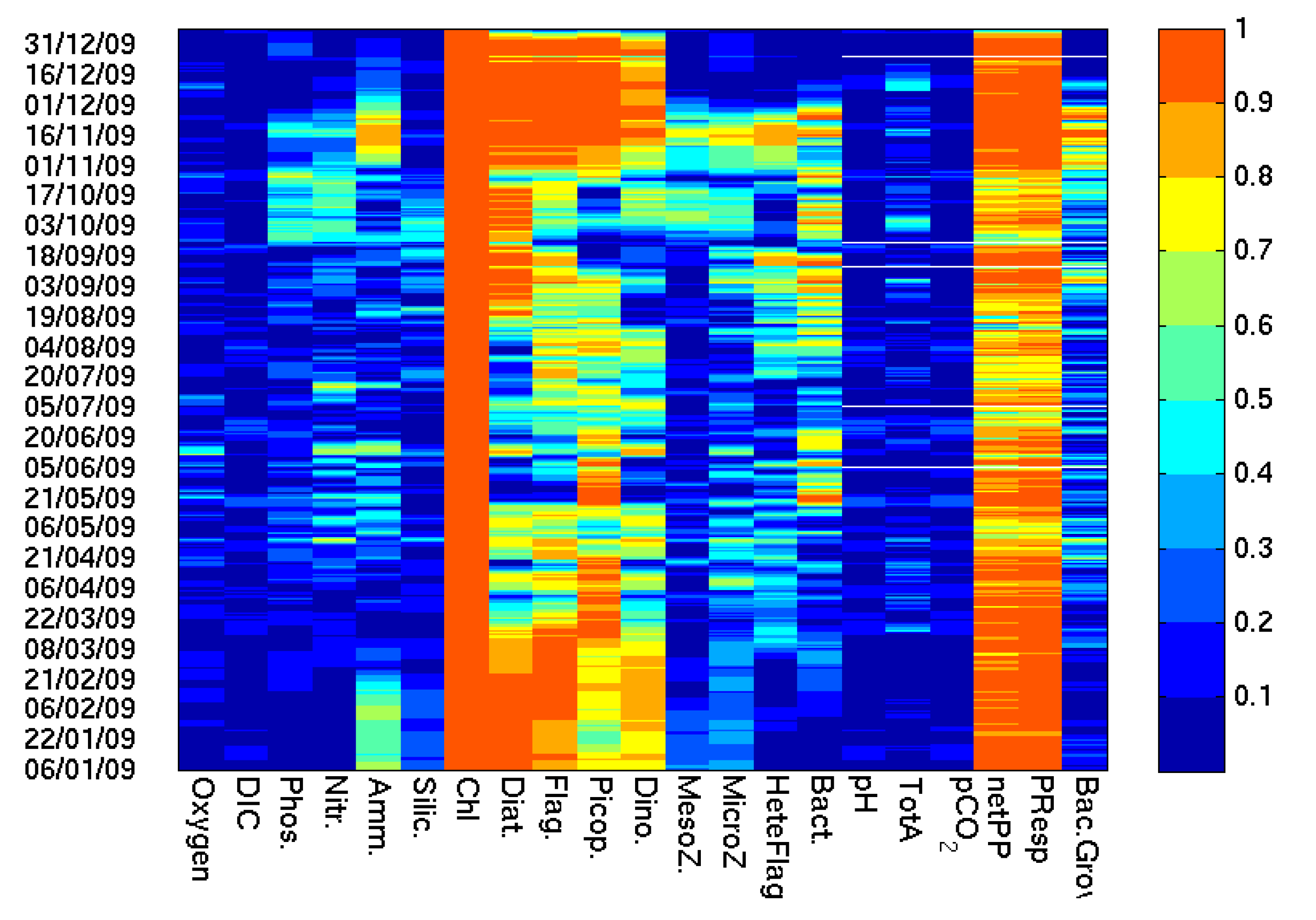
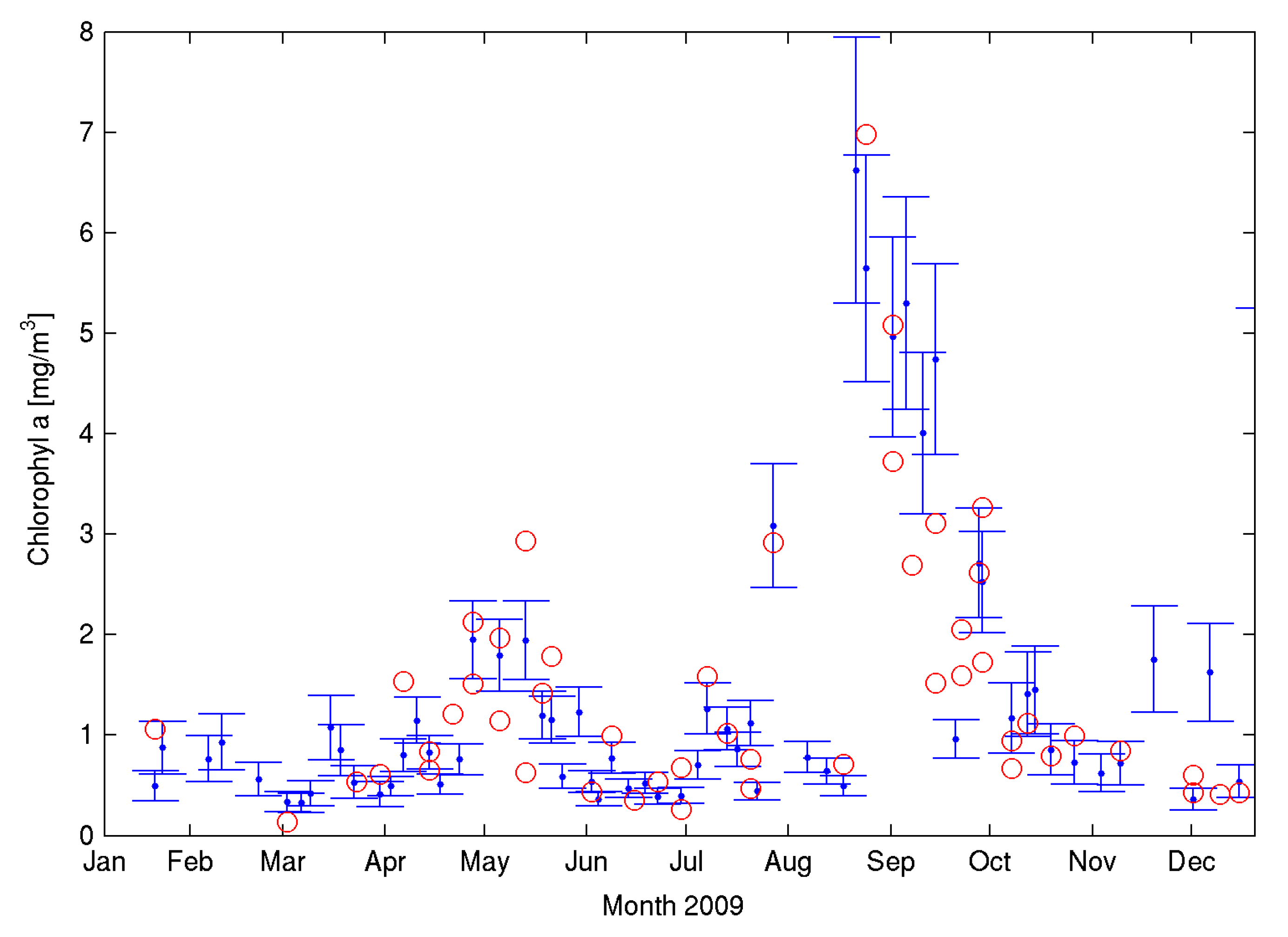
The in situ observations used in this work have been extensively described in numerous papers (e.g., [16,17,37,45]) but we provide a brief overview here. The seasonality of nutrients show typical maximum values in January (8 μM m⁻³ for Nitrate, 0.5 μM m⁻³ Phosphate, 5 μM m⁻³ Silicate) and minima after the spring bloom (from May) until it starts increasing again in September following the weakening of the thermal stratification. Chl-a also shows a marked seasonality at L4 (e.g., Figure 1). Two peaks are identified year on year in the data, one coincidental with the spring bloom (April–May) and one in September–October. The spring bloom is generally dominated by diatoms but with significant contributions from coccolitophores and phaeocystis. The analysis of 15 years of phytoplankton abundance at L4 [16] has shown significant seasonal and inter-annual changes in abundance and composition although seasonality is the largest determinant of these changes. The authors found that the winter community seems relatively stable over the years. The spring period represents the largest change event in both composition and abundance while the summer period is the most susceptible to inter-annual changes in composition [16]. Overall, flagellates are the dominant group representing 87% of the total phytoplankton cell abundance on average with the smaller cells (2–4 μm) accounting for 63% of the total abundance. In terms of biomass, they represent a small but significant proportion of the total biomass.

3.1. Reference Simulation; Experiment A

3.1.1. Physics

We have evaluated both the model capacity to reproduce the seasonal changes in the physical environment as well as sub-daily changes associated with the semi-diurnal tides. Initial calibration of the model and simulations to evaluate the sensitivity of the model to variations in forcing have been performed for the years 2009–2010, when data from the oceanographical buoy are available and can help to reduce uncertainty in the meteorological forcing. In August 2010, we deployed a bottom mounted Teledyne RD Instruments 600 kHz Broadband Acoustic Doppler Current Profiler (ADCP) at L4 for 20 days [61].

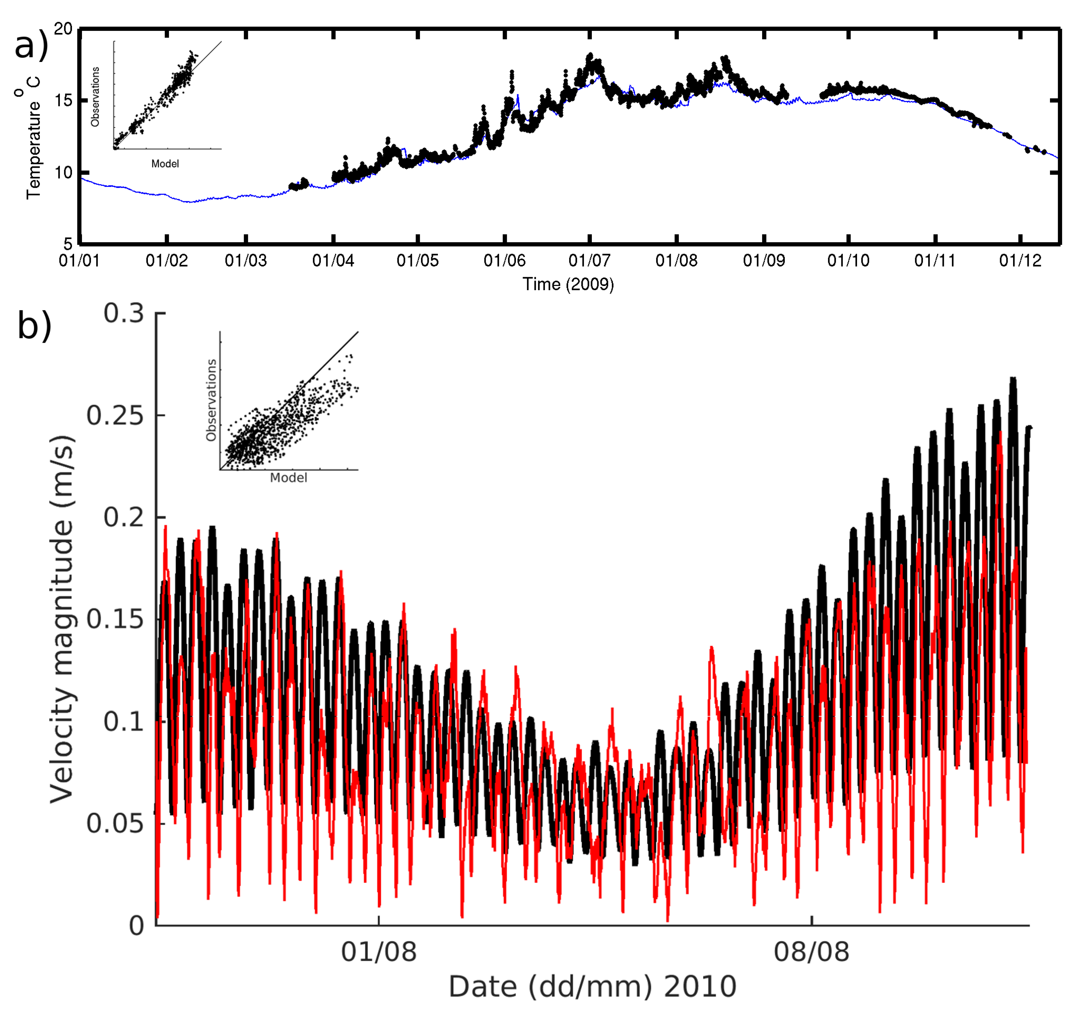
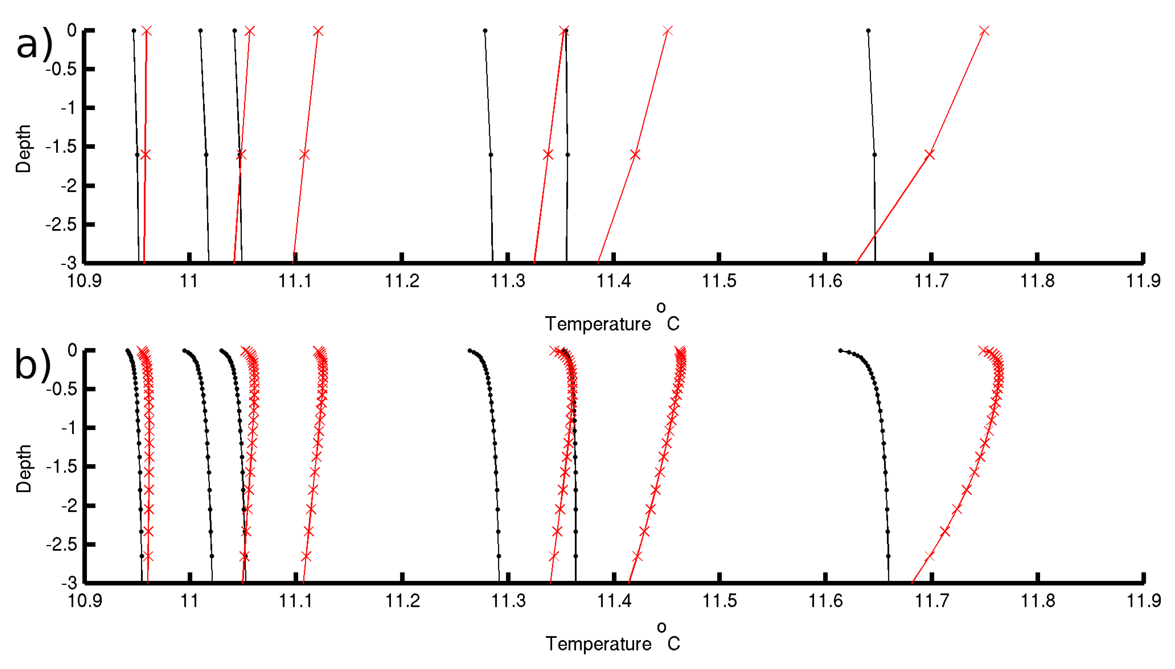
The seasonality in hydrography is well reproduced by the model (Figure 2a). This arises partly from the fact that we are using a basic nudging technique to relax the model temperature (T) and salinity (S) to the observed CTD profiles with a relaxation time of two weeks. The correlation for near-surface (1.5 m) temperature between the independent observations from the L4 monitoring buoy and the model was larger than 0.9 and significant at the 99.9% confidence level (full statistics can be found in

Table A4. Pearson correlations for experiments A–D, between observed and modeled variables for 2008–2009 at the shallowest depth available. Significant correlations at the 95% are indicated by *.

Exp	Year	Variable	Depth	Corr	p Value	RMSE	Mean	Std	N
Exp A	2008	DIC	2	0.46 *	0.011	91.08	2162.59	13.47	30
Exp A	2009	DIC	2	0.47 *	0.020	79.90	2140.67	21.76	25
Exp B	2008	DIC	2	0.51 *	0.005	100.20	2172.67	14.11	30
Exp B	2009	DIC	2	0.54 *	0.006	78.60	2138.66	26.56	25
Exp C	2008	DIC	2	0.46 *	0.010	90.88	2162.38	13.50	30
Exp C	2009	DIC	2	0.47 *	0.020	79.85	2140.63	21.78	25
Exp D	2009	DIC	2	0.30 *	0.040	61.35	2117.08	13.29	46
Exp A	2008	pCO2	2	0.52 *	0.003	74.81	401.57	31.42	30
Exp A	2009	pCO2	2	0.41 *	0.042	42.53	353.65	28.97	25
Exp B	2008	pCO2	2	0.62 *	0.000	88.12	425.92	31.84	30
Exp B	2009	pCO2	2	0.35	0.086	44.64	350.10	33.64	25
Exp C	2008	pCO2	2	0.52 *	0.003	74.51	401.13	31.45	30
Exp C	2009	pCO2	2	0.41 *	0.042	42.48	353.57	28.98	25
Exp D	2009	pCO2	2	−0.20	0.176	37.39	329.72	17.27	46
Exp A	2008	pH	2	0.53 *	0.002	0.09	8.04	0.03	30
Exp A	2009	pH	2	0.38	0.060	0.06	8.09	0.03	25
Exp B	2008	pH	2	0.63 *	0.000	0.11	8.02	0.03	30
Exp B	2009	pH	2	0.33	0.108	0.06	8.09	0.03	25
Exp C	2008	pH	2	0.53 *	0.002	0.09	8.04	0.03	30
Exp C	2009	pH	2	0.38	0.060	0.06	8.09	0.03	25
Exp D	2009	pH	2	−0.22	0.143	0.05	8.12	0.02	46
Exp A	2009	SST	1.5	0.94 *	0.000	0.54	13.74	2.13	903
Exp B	2009	SST	1.5	0.93 *	0.000	0.53	13.82	2.15	903
Exp C	2009	SST	1.5	0.94 *	0.000	0.54	13.74	2.13	903
Exp D	2009	SST	1.5	0.91 *	0.000	0.57	13.91	2.13	4809

).

The ability of the model to reproduce the velocity structure was evaluated during a simulation of the August ADCP deployment. The results indicate that the model setup reproduces the barotropic component of the tidal velocity well considering the 1D approach. The correlation between the depth mean averaged velocity between 2 and 30 m was 0.7 at the 99.9% confidence level. The dominant E–W component is better resolved albeit with a small overestimation of the flood peak velocity (correlation of 0.9 at 99.9% confidence level). The N–S component shows a larger amplitude in magnitude than the observations which resulted in lower correlations of 0.7. The velocities closest to the bottom (averaged between 1 and 2 m above the seabed, (Figure 2b)) have a better agreement between model and observations with an overall correlation of 0.8 for the velocity magnitude. As it is a tidally dominated station, this is key to ensuring a realistic level of mixing is imposed to the biological model.

3.1.2. Biogeochemistry

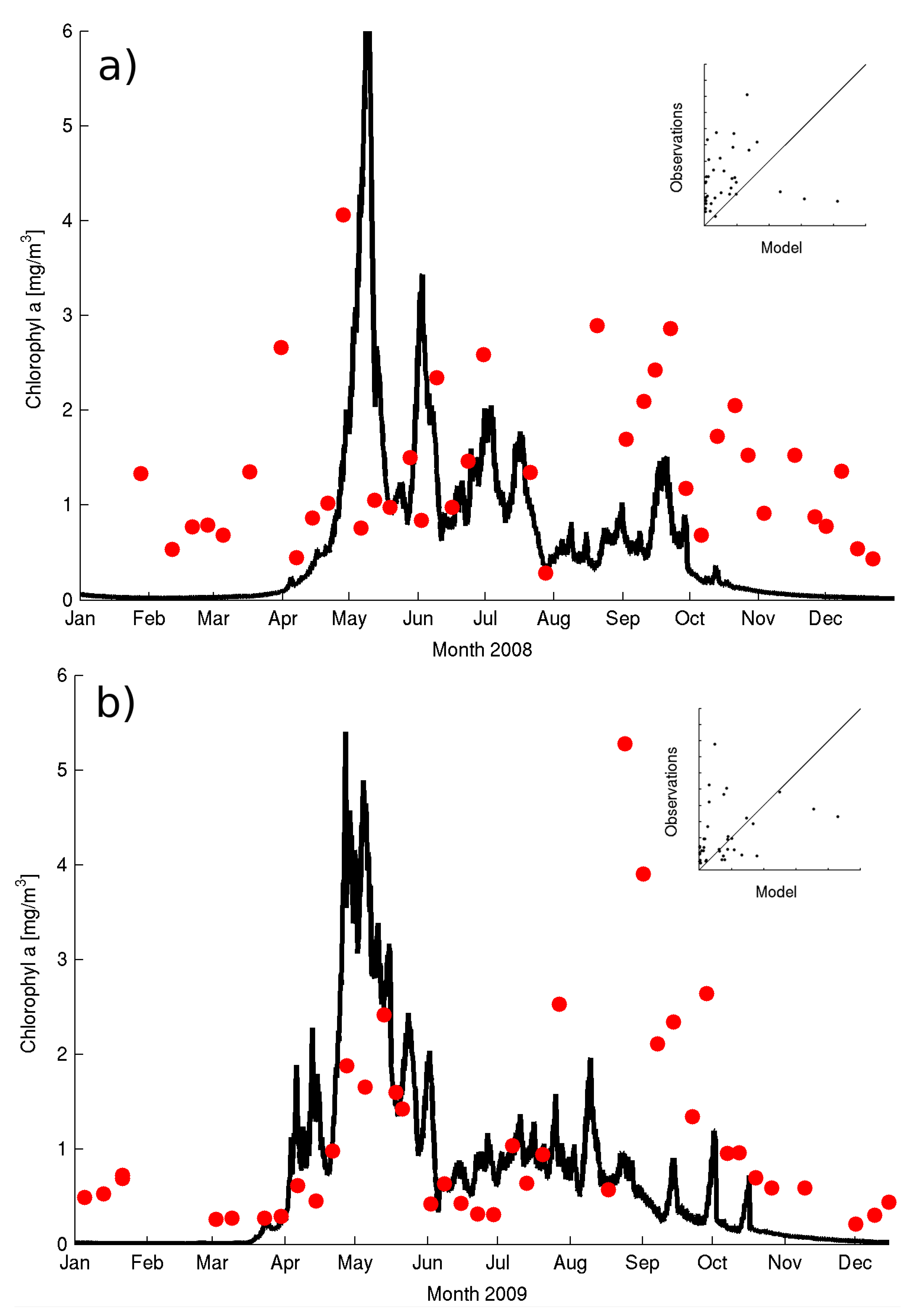
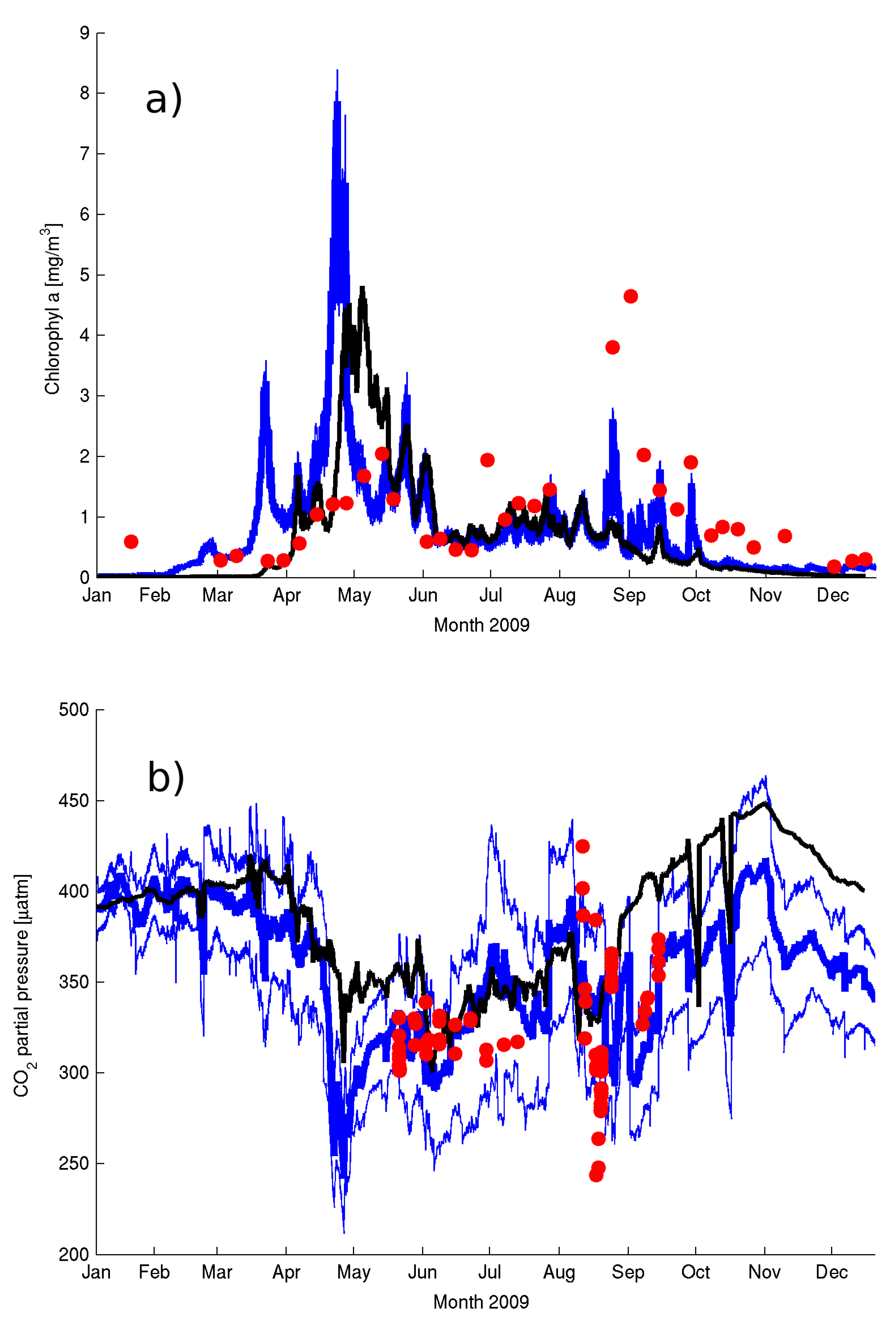
The model output at six hourly intervals in 2008–2009 at the sampling depth of 10 m (Figure 3a,b) shows the model correctly reproduces the approximate timing and duration of the spring bloom. The model indicates a short sharp spring bloom in 2008 (Figure 3a) with subsequent short-lived blooms during June–July in agreement with the available observations. The spring bloom in 2009 is by contrast longer (Figure 3b) although the model overestimates the chl-a concentrations. Nonetheless, the observations suggest a substantial overestimation of diatom biomass in 2008 (Figure 4b) but the correct order of magnitude in May 2009 (Figure 4b). The model underestimates total chl-a from January to mid-April and from September to December in 2008 and 2009. The main discrepancy with the observations is the late dinoflagellate bloom (not shown) which the model underestimate in both years although the miss-match is most evident in 2009 (Figure 3b).

The main functional group responsible for the winter surface chl-a and spring bloom is diatoms (Figure 4a,b) with a significant contribution from flagellates (Figure 4c) which ranges from maximum of 40% during the spring bloom to 10–20% during the summer months.

The modeled spring bloom has knock-on effects in the simulated plankton succession. The collapse of the spring bloom generates substantial concentrations of ammonium which in turn triggers the onset of a succession of summer picoplankton blooms. The small pico-phytoplankton functional group dominates both chl-a and net production. Their higher affinity for ammonium and faster growth enables them to out compete both diatoms and flagellates and they are responsible for the disappearance of surface nutrients. The short-lived blooms in Figure 3 are both a consequence of the variability in the observed irradiance and the model dynamics of nutrient–prey–predator cycles. The largest chl-a values are however not at the surface but in the well-developed subsurface chl-a maximum [62].

Total biomass, here considered to be the sum of diatoms, flagellates and dinoflagellates, agrees well with the observations (

Table 1. Pearson correlations for simulation experiments A–D, between observed and modeled variables for 2008 and 2009 at the shallowest depth available. Significant correlations at the 95% are indicated by *. Values in italic signify an improvement with respect to Experiment A.

Year	Total Chl	Total C	Silicate	Nitrate	Phosph.	Ammon.	DIC	pCO2	Ph
Exp A
2008	0.43 *	0.70 *	0.82 *	0.90 *	0.82 *	−0.23	0.46 *	0.52 *	0.53 *
2009	0.45 *	0.76 *	0.86 *	0.90 *	0.77 *	−0.46 *	0.47 *	0.41 *	0.38
Exp B
2008	0.41 *	0.67 *	0.83 *	0.92 *	0.87 *	−0.35 *	0.51 *	0.62 *	0.63 *
2009	0.48 *	0.75 *	0.86 *	0.88 *	0.90 *	−0.46 *	0.54 *	0.35 *	0.33 *
Exp C
2008	0.43 *	0.70 *	0.82 *	0.90 *	0.82 *	−0.23	0.46 *	0.52 *	0.53 *
2009	0.45 *	0.76 *	0.86 *	0.90 *	0.77 *	−0.46 *	0.47 *	0.41 *	0.38
Exp D
2009	0.46 *	0.49 *	0.86 *	0.90 *	0.88 *	−0.40 *	0.30 *	−0.20 *	−0.22

) from April to August with the largest discrepancy observed at the time of a mono-specific dinoflagellate bloom in early September 2009. These mono-specific blooms are one of the best-known weaknesses in biogeochemical models that embrace a functional group approach [63]. 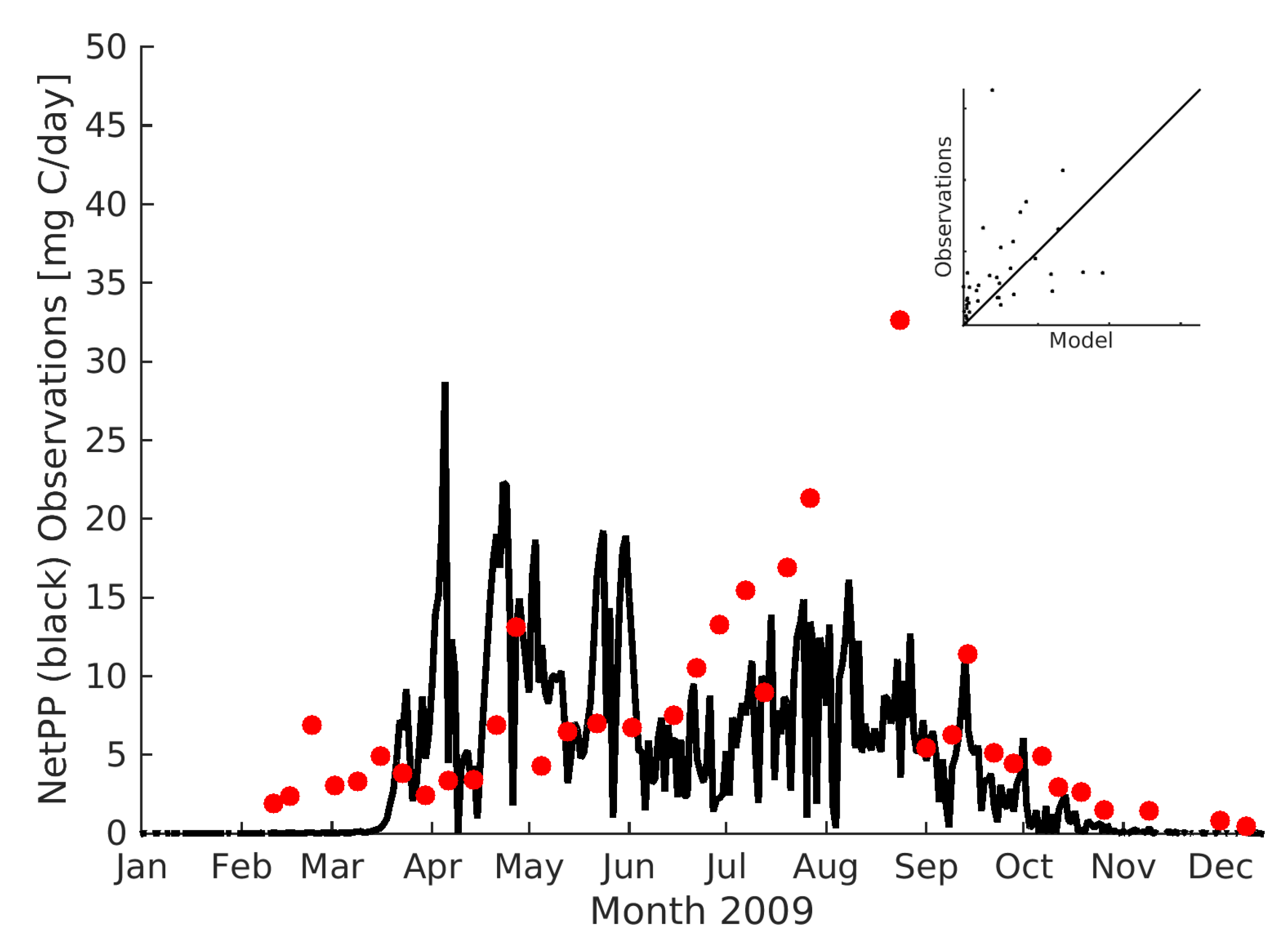Despite the model shortcomings, we still resolve the observed total biomass seasonality with correlations larger than 0.7 in both years (see Table 1). The daily and depth integrated net primary production (Figure 5) has a lower correlation of 0.6 (see

Table A1. Pearson correlations for experiments A–D, between observed and modeled variables for 2008–2009 at the shallowest depth available. Significant correlations at the 95% are indicated by *.

Exp	Year	Variable	Depth	Corr	p Value	RMSE	Mean	Std	N
Exp A	2008	Biomass	10	0.70 *	0.000	99.59	21.91	42.81	40
Exp A	2009	Biomass	10	0.76 *	0.000	119.83	17.85	33.54	41
Exp B	2008	Biomass	10	0.67 *	0.000	98.91	19.95	37.18	40
Exp B	2009	Biomass	10	0.75 *	0.000	120.41	17.36	34.76	41
Exp C	2008	Biomass	10	0.70 *	0.000	99.71	21.99	43.05	40
Exp C	2009	Biomass	10	0.76 *	0.000	119.83	17.85	33.54	41
Exp D	2009	Biomass	10	0.49 *	0.001	119.58	23.32	37.84	42
Exp A	2009	Chl-a	0	0.47 *	0.003	1.28	0.78	0.95	38
Exp B	2009	Chl-a	0	0.50 *	0.002	1.29	0.81	1.00	38
Exp C	2009	Chl-a	0	0.47 *	0.003	1.28	0.78	0.95	38
Exp D	2009	Chl-a	0	0.46 *	0.003	1.39	0.95	1.15	40
Exp A	2008	Chl-a	10	0.43 *	0.005	2.42	0.65	0.87	41
Exp B	2008	Chl-a	10	0.41 *	0.008	2.42	0.66	0.88	41
Exp C	2008	Chl-a	10	0.43 *	0.005	2.42	0.66	0.88	41
Exp A	2009	Chl-a	10	0.45 *	0.004	1.27	0.76	0.95	39
Exp B	2009	Chl-a	10	0.48 *	0.002	1.28	0.79	1.00	39
Exp C	2009	Chl-a	10	0.45 *	0.004	1.27	0.76	0.95	39
Exp D	2009	Chl-a	10	0.50 *	0.002	1.29	0.95	1.09	37
Exp A	2009	Chl-a	50	0.63 *	0.000	0.45	0.29	0.46	33
Exp B	2009	Chl-a	50	0.63 *	0.000	0.45	0.28	0.45	33
Exp C	2009	Chl-a	50	0.63 *	0.000	0.45	0.29	0.46	33
Exp D	2009	Chl-a	50	0.32	0.054	0.46	0.30	0.21	36
Exp A	2009	Primary production	10	0.40 *	0.015	23.51	17.50	23.95	36
Exp B	2009	Primary production	10	0.39 *	0.018	17.22	10.34	15.05	36
Exp C	2009	Primary production	10	0.40 *	0.015	23.51	17.50	23.95	36
Exp D	2009	Primary production	10	0.42 *	0.010	32.16	23.81	32.09	38

).

Nonetheless, smaller blooms of diatoms are still reproduced in the model simulations with a good agreement with the observations (Figure 4a). The observed phytoplankton production (PP) at 10m indicates a strong seasonality with maximum values during July August (e.g., Figure 5). In contrast, the model suggests a high PP during both the spring bloom and the summer months of July and August.

All the measured surface nutrients display a strong seasonal signal which is captured by the model (e.g., Figure 6a,b) with the exception of ammonium (

Table A3. Pearson correlations for experiments A–D, between observed and modeled variables for 2008–2009 at the shallowest depth available. Significant correlations at the 95% are indicated by *.

Exp	Year	Variable	Depth	Corr	p Value	RMSE	Mean	Std	N
Exp A	2008	Phosphate	1	0.84 *	0.000	0.17	0.39	0.16	39
Exp A	2009	Phosphate	1	0.90 *	0.000	0.19	0.39	0.16	41
Exp B	2008	Phosphate	1	0.87 *	0.000	0.19	0.42	0.16	39
Exp B	2009	Phosphate	1	0.90 *	0.000	0.21	0.42	0.16	41
Exp C	2008	Phosphate	1	0.84 *	0.000	0.17	0.39	0.16	39
Exp C	2009	Phosphate	1	0.90 *	0.000	0.19	0.39	0.16	41
Exp D	2009	Phosphate	1	0.88 *	0.000	0.24	0.47	0.18	43
Exp A	2008	Nitrate	1	0.90 *	0.000	2.29	5.04	2.68	40
Exp A	2009	Nitrate	1	0.90 *	0.000	2.54	4.99	2.79	42
Exp B	2008	Nitrate	1	0.92 *	0.000	2.66	5.50	2.65	40
Exp B	2009	Nitrate	1	0.88 *	0.000	2.89	5.37	2.75	42
Exp C	2008	Nitrate	1	0.90 *	0.000	2.29	5.04	2.68	40
Exp C	2009	Nitrate	1	0.90 *	0.000	2.54	4.99	2.79	42
Exp D	2009	Nitrate	1	0.90 *	0.000	2.40	4.98	3.00	44
Exp A	2008	Ammonium	1	−0.23	0.156	0.59	0.46	0.35	39
Exp A	2009	Ammonium	1	−0.46 *	0.002	0.63	0.46	0.38	41
Exp B	2008	Ammonium	1	−0.35 *	0.031	0.70	0.51	0.45	39
Exp B	2009	Ammonium	1	−0.46 *	0.003	0.71	0.51	0.48	41
Exp C	2008	Ammonium	1	−0.23	0.156	0.59	0.47	0.36	39
Exp C	2009	Ammonium	1	−0.46 *	0.002	0.63	0.46	0.38	41
Exp D	2009	Ammonium	1	−0.40 *	0.008	0.67	0.61	0.40	43
Exp A	2008	Silicate	1	0.82 *	0.000	1.95	4.42	2.04	37
Exp A	2009	Silicate	1	0.86 *	0.000	2.17	4.47	1.97	41
Exp B	2008	Silicate	1	0.83 *	0.000	1.99	4.49	1.94	37
Exp B	2009	Silicate	1	0.86 *	0.000	2.15	4.45	1.98	41
Exp C	2008	Silicate	1	0.82 *	0.000	1.95	4.42	2.03	37
Exp C	2009	Silicate	1	0.86 *	0.000	2.17	4.47	1.97	41
Exp D	2009	Silicate	1	0.86 *	0.000	1.73	4.15	2.04	43

). The main discrepancies relate to the rapid consumption of nutrients (silicate, nitrate and phosphate) during the spring bloom and the low nutrient concentrations during the summer period (mid-May to early September). The observations suggest that diatoms start drawing dissolved silicate from February (Figure 6a) decreasing steadily until mid-April followed by a sharp drop to limiting levels by mid-late June. The early slow growth is likely controlled by light limitation and possibly by weak predation pressures. The sharp end of the bloom in May is potentially the result of predation from mesozooplankton. Light is a key driver of the pelagic ecosystem which during the winter period is dominated by the natural low levels at this northern latitude and the local re-suspension of benthic sediments, a process not resolved in the present GOTM–ERSEM implementation. Our hypothesis is that light limitation is responsible for the overestimation in the modeled biomass during the spring bloom with respect to the observations.

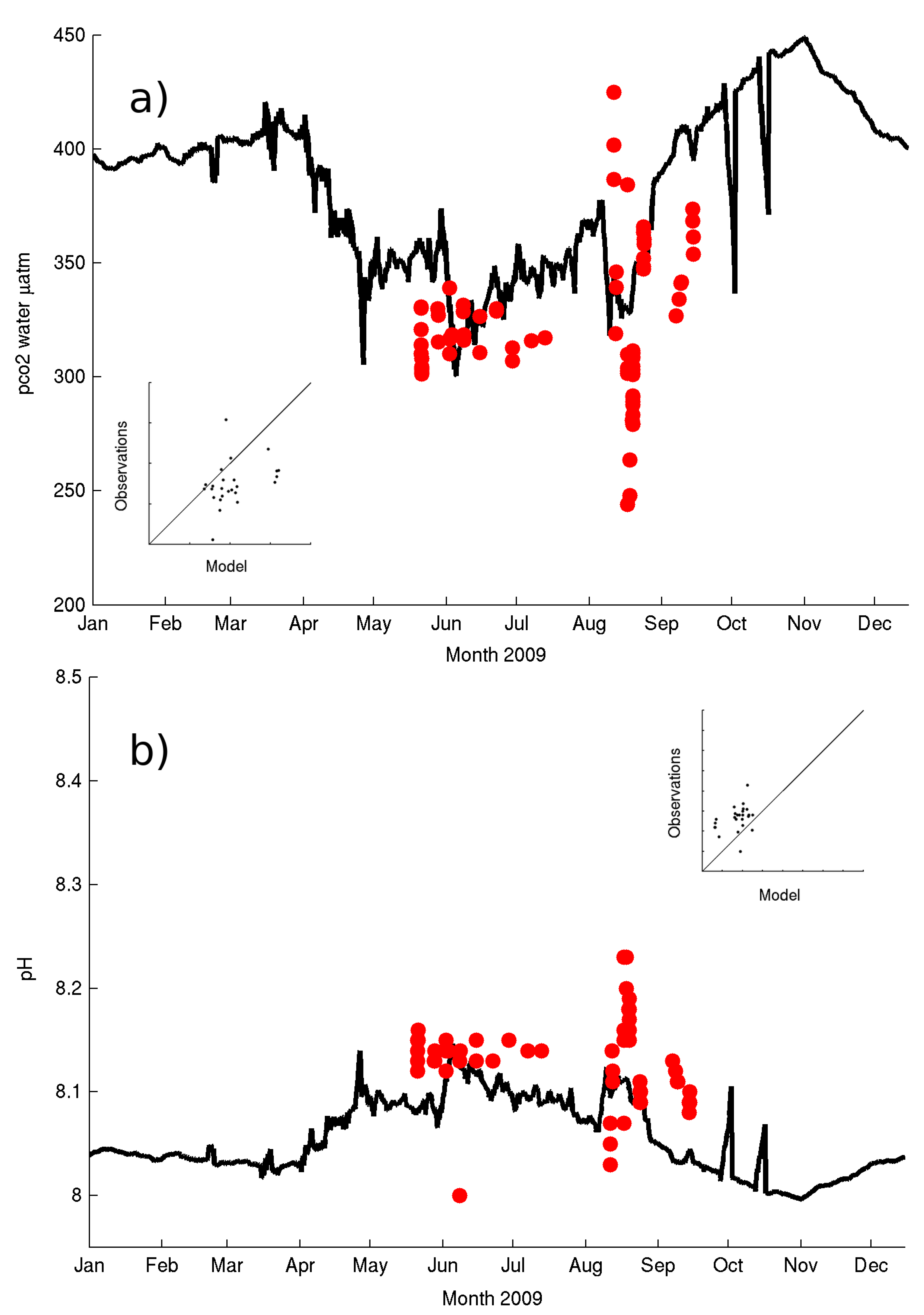
The evolution of the observed variables related to the carbonate system at the surface (namely pH and CO₂ partial pressure [pCO₂] ) follow the available data for 2008 and 2009 although the model underestimates the large daily fluctuations that can be seen in the data (Figure 7a,b). The seasonal signal described in Kitidis et al. [45] of increased pCO₂ and low pH in winter and autumn (October to March) and low pCO₂ and high pH during summer and spring (April to September) is well reproduced by the model in all years. The range in the observed values is also well captured by the model (~200 μatm for pCO₂ and ~0.15 pH units). Both model and observations show increased variability during the summer/stratified periods strongly coupled to phytoplankton blooms with timescales of 1–3 weeks.

3.2. Enhance Surface Resolution; Experiment B

To evaluate the effect of resolving the diurnal cycle of the near-surface temperature on the air–sea fluxes we modified the baseline experiment by changing the vertical setup. The vertical grid is enhanced at the surface, and the resolution increased logarithmically from 2 cm at the surface to 1 m at 10 m deep. The water column interior (between 10 m deep and 35 m deep) has the same nominal resolution of the reference experiment (1.6 m). This setup resolves the diurnal cycle of temperature associated with the near-surface layer (e.g., Figure 8b) [64]. During effective heat loss at the sea surface from high winds or cooler air temperature than sea-surface temperature the shallowest ∼20 cm have a negative temperature gradient both during day and night time (Figure 8b) that was not resolved in Experiment A (Figure 8a). The absorption of incoming solar radiation takes place over the top several meters of the water column, but heat is released right at the surface which causes the very surface to cool. During daytime, a subsurface temperature maximum develops between 30 and 150 cm (80 cm on average) from the surface. The largest differences between the two experiments concentrate on the top 3 m, below which depth the root mean square error (RMSE) decreases to 50% of the surface value (RMSE = 0.17 °C). The RMSE decrease flattens at 12 m and remains at 10% of the surface value to the bottom.

The development of the very near-surface gradient results in changes to the amplitude of the daily fluctuations of temperature such that the night–day range reduces in Experiment B, making night time minima warmer and day time maxima cooler than in Experiment A as the near-surface gradients limit the exchange of heat with the atmosphere.

pCO₂ shows a similar night–day evolution to the temperature profiles with a consistent negative gradient in the top 20 cm and the development of a daytime subsurface maximum coincidental with the temperature maximum.

Experiment B showed that the carbonate system model variables are sensitive to the increased resolution near the surface. The comparison between experiments A and B (Table 1) shows the largest improvements in 2008, in particular for pH, pCO₂ and DIC (a 10%, 19% and 18% improvement respectively, Table 1). The effect on the air–sea flux is largest and it is apparent throughout the year save the most stratified periods between June and August. The impact is important and results in a 70% to 100% increase in the net CO₂ uptake at L4. The modeled integrated annual CO₂ flux was 1.8 mo C/m²/year in Experiment A for 2008 increasing to an integrated annual CO₂ flux of 2.8 mo C/m²/year in Experiment B for the same year. A similar result is obtained for 2009 with a change from net CO₂ source of 0.3 mo C/m²/year in Experiment A to net CO₂ source of 0.6 mo C/m²/year in Experiment B.

3.3. Evaluation of Surface Slicks; Experiment C

Experiment C involved a parameterization of the effects of primary production on the CO₂ transfer velocity ($K_{C{O}_2}$). This was introduced through a scaling $K_{C{O}_2}$ with the gross primary production excreted by the phytoplankton as a result of its metabolic activity. In practice, $K_{C{O}_2}$ was reduced to a maximum of 70% of its wind dependent value (calculated following Nightingale et al. [65]) when the gross productivity surpasses the 30% highest values modeled at L4 in the years 2008–2009. The results are summarized in Table 1 and suggest a negligible impact when compared to Experiment A. The integrated annual CO₂ flux supports these results with changes smaller than 1% for both 2008 and 2009 years.

3.4. Evaluation of Data Assimilation; Experiment D

Results from Experiment D show that assimilation of EO chl-a improves some of the model variables but it also deteriorates bulk variables like total biomass (Table 1 and Table A1 in Appendix A). As expected from previous work [34] the forecast step always shows a larger variance or ensemble spread than after the analysis step suggesting a reduction in ensemble variance as a result. The modeled mixed layer chl-a (Figure 9a) shows an improved agreement with observations (Table 1) but the model fails to capture the spring bloom correctly. In particular, the model solution constructed as the mean of all the model ensembles overestimates chl-a in March and end of April while the overestimation during the observed spring bloom in May improves. The summer evolution of chl-a is better resolved as is the increase seen in September (Figure 9a).

The improvement seen in chl-a do not however translate to a better fit in modeled total biomass, and the assimilation of chl-a degrades the model solution as a result of the large miss-representation of the spring bloom (not shown). Indeed, when the results between 15 March and 15 April are removed, the correlation for total biomass increases to 0.61 at the 95% significance. One effect of the assimilation is the overestimation of all the nutrient variables during the spring bloom (not shown). This reflect the inability of the model to lower the chl-a field without increasing the nutrient values during that period. The discrepancies and excess nutrients are however corrected during the summer period and have a small impact on the overall correlation with observations (Table 1).

It is, however, noteworthy that while the correlations with observations of all variables in the carbonate system (pH, DIC and pCO₂, Table 1) do not improve, the bias or RMSE is significantly reduced (Table A4). The ensemble variance was reduced in the modeled chl-a as a result of the assimilation but it is apparent in Figure 9b that this is not the case for pCO₂ or DIC and pH (not shown), although after the initial increase during the first three months of the experiment, it is also true that it did not increase monotonically.

4. Discussion

4.1. Ecosystem Models Predictive Capabilities of CO₂

We have shown that a 1D approach using GOTM–ERSEM captures the seasonality of the pelagic ecosystem at L4, including the variables driving the air–sea exchange of CO₂ (e.g., year 2008 Table 1). The results from year 2009 (Table 1) suggest that the model’s ability to simulate the total biomass and nutrients is not a sufficient condition to resolve the surface evolution of DIC and pCO₂. This follows the poorer simulation of chl-a in 2009 and suggests that an adequate simulation of chl-a and the associated plankton production and respiration rates is critical for a better estimation of the CO₂ dynamics. The seasonality and range of simulated DIC and pCO₂ agree with recent observations [45] and suggest both a physical and biological control. 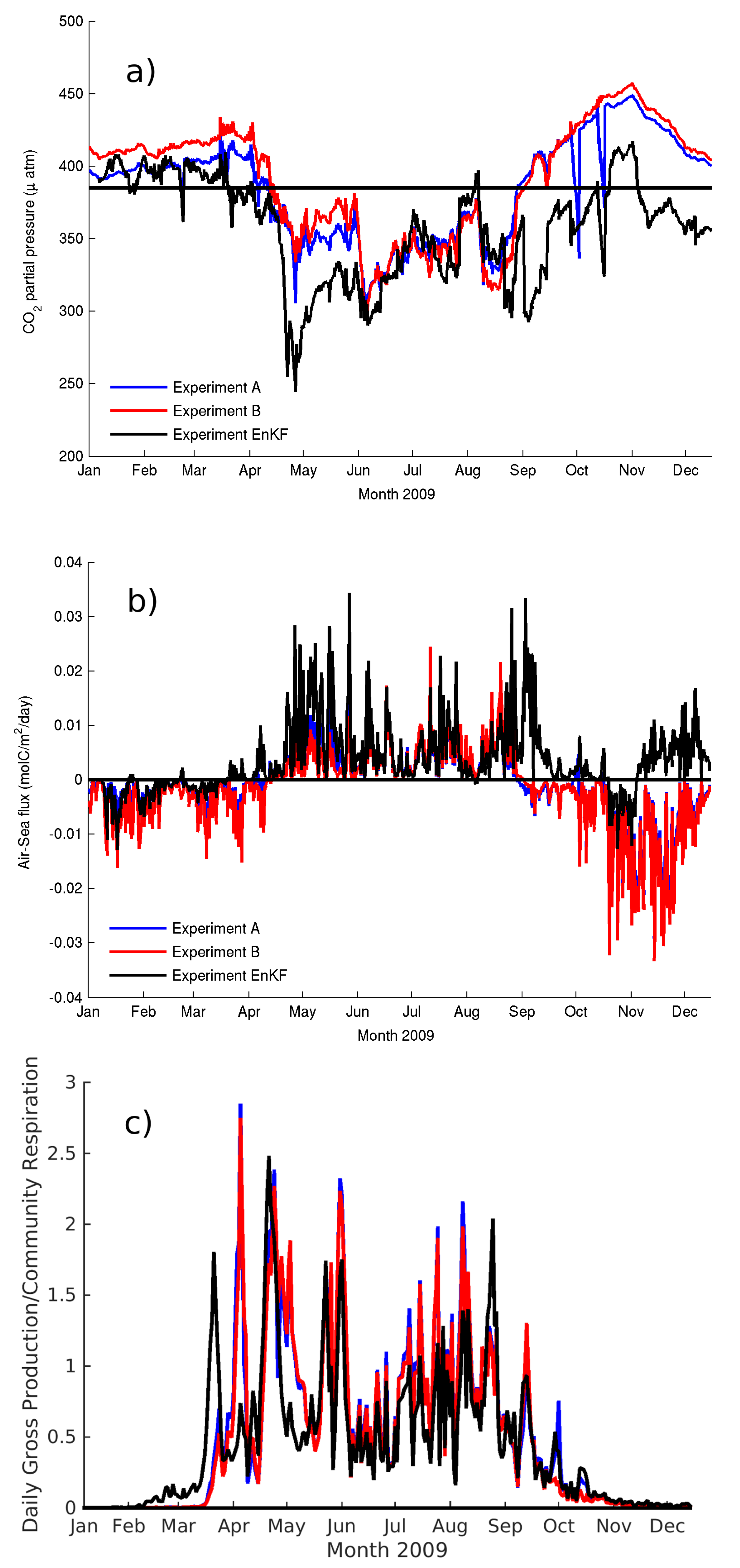The high production during the spring and summer periods (Figure 5) produces undersaturation of CO₂ (Figure 10a) resulting in a net sink of CO₂ into the waters. It is worth noting that the short-term variability in air–sea CO₂ fluxes is as high as the seasonal signal (Figure 9a) and that the summer blooms can drive a similar exchange to the longer spring bloom.

Despite the model’s ability to capture the seasonal cycle on all the variables of the carbonate system the model seems to underestimate the short-term variability seen in the data (Figure 9b). This can be related to the coarse temporal resolution of the wind forcing (six hourly) (e.g., [64]) and the effect of lateral advection which is intrinsic in the data and not resolved in the model. At L4, variations in DIC drive the observed variability in the carbonate system and thus pCO₂ as total alkalinity has very low variability [45]. The model solution suggests that L4 can be considered a neutral site with respect to CO₂ fluxes or a small source (

Table 2. Air-sea flux annual integrated values for each of the experiments.

Experiment	Air-Sea Flux of CO2 in molC/m2/day
	2008	2009
Exp A	−1.8	−0.3
Exp B	−2.8	−0.6
Exp C	−1.8	−0.3
Exp D		1.3 ± 1.7

) in contrast to the results reported by Kitidis et al. [45].

4.2. Sensitivity of Modeled CO₂ to SST Diurnal Cycle

The increased vertical resolution near the surface in Experiment B enabled the simulation of the diurnal cycle in SST [64] which overall had a small impact on the ability of GOTM–ERSEM to simulate the bulk properties of the pelagic ecosystem at L4 as observed at 10 m (Table 1) but a large impact on the air–sea fluxes of CO₂ (Figure 10a,b). The comparison with SST measured at the L4 buoy yielded a small decrease in correlation (from 0.94 to 0.93 at the 99.9% confidence level) and a small decrease in the bias (see Table A4). Experiment B did however improve the simulation of pCO₂, DIC and pH in 2008. The largest differences in the carbonate system between experiments A and B in 2009 concentrated in the first 5 months (January to May, Figure 10a) and in Experiment B resulted in an increased supersaturation and resulting flux to the atmosphere from January to March. The amplitude of the daily variations in the fluxes remained relatively unchanged from June to December (Figure 10b) driven primarily by the daily fluctuations in productivity. The difference was largest during the low productivity months of January to March and it was partly responsible for the change in value of the net flux estimates.

The changes with respect to the reference experiment (A) are mostly located in the top 10 m and decrease with depth in a significant number of variables (Figure 11). These include rate variables like respiration and production as well as state model variables like biomass of plankton and zooplankton. These differences will be discussed in relation to three periods in 2009 defined as a winter non-growing season (January to March with a consistent gross production to community respiration (G/R) ratio less than one, Figure 10c), the summer growing season from April to August (G/R averaging one or above) and the autumn non-growing season with G/R again less than one.

Most of the variables evaluated changed between 0.1% to 6% except for gross production and community respiration that showed increases between 26 and 34% in all seasons. Experiment B displayed a small increase in temperature in the top 10m throughout the year (0.1%) increasing to 0.5% during the growing season. Total detritus (the sum of the three classes in ERSEM, small, medium and large) decreased in the winter (4%), while on averaged did not change during summer and decreased by 5% in the autumn in Experiment B. Irradiance levels also increased in Experiment B (5% in all seasons) in response to a decrease in biomass of 2% in winter and 6% in autumn).

In general, though, pCO₂ increased in Experiment B in both growing and non-growing season by 2%. During the non-growing season, this translates into an increase release of CO₂ to the atmosphere in both 2008 and 2009. During the growing season, there is no one specific trend, as the CO₂ exchange with the atmosphere depends on both the biological uptake of CO₂ as well as the wind. During the two years evaluated, in 2009 there was no overall change while in 2008, there was a larger release of CO₂ in Experiment B.

4.3. Sensitivity of Modeled CO₂ to Surface Surfactants

The reduction of the gas transfer velocity ($K_{C{O}_2}$) as a function of sea-surface surfactants had a very small impact on the integrated annual CO₂ flux (Table 2) and bulk ecosystem variables (Table 1) in our modeled site compared to the results of experiments B and D (Section 3.2 and Section 3.4). This is both a consequence of our choice of parameterization (Section 3.3) of the production of surfactant material and the environmental characteristics of our site. The large variability in phytoplankton gross production (similar to phytoplankton net production in Figure 5) implies that the reduction of $K_{C{O}_2}$ is only active during a small proportion of the time (<5% during 2008–2009) between April–September and results in small reductions of $K_{C{O}_2}$ (<1%). The high average wind speed (~8 ${\mathrm{ms}}^{-1}$ observed at L4 in 2008–2009 also limits the impact of the surfactants on the annual integrated fluxes. This contrasts with the findings of Pereira et al. [52] who reported an overall 9% reduction in the net CO₂ flux integrated over the entire Atlantic Ocean basin in 2014. Nonetheless, their analysis showed that at our latitude (although no estimates are presented for the UK shelf) the decreased surfactant suppression was consistently less than 5% except for July–September when it increased to 10%.

4.4. Sensitivity of Modeled CO₂ to the Assimilation of chl-a

The assimilation of chl-a had a significant impact in the carbonate system but mostly by reducing the bias in DIC, pH or pCO₂. The correlations deteriorated for all three variables but the concentration of the observations around the May to September months precludes a definitive assessment of the effect of surface chl-a assimilation on simulating the seasonality of the carbonate system. Experiment D also corrected the simulation of chl-a and the nutrients silicate and phosphate (Table 1).

Similar to Experiment B, Experiment D had a significant impact on the top 10 m averaged G and R, particularly during the winter (G increased 450%, R 20%) and in autumn (G increased 60% R 23%). Off all the variables evaluated, only plankton biomass had similar changes with a 900% increase in winter compared to 70% increase in the autumn. The second largest corrections corresponded to the zooplankton biomass, which decreased in winter (28%) and in summer (10%) while it increased in autumn (53%). Generally, the growing season saw more modest changes across all variables between 3 and 12%. It is worth remembering that although the percentage increases are significant they represent a small number as they correspond to the non-growing seasons (winter in particular) when biomass levels and carbon uptake and respired are very small. This is a further indication that winter ecosystem dynamics and autumn ones are the least well captured by this 1D model approach.

One way of visualizing how the information associated with chl-a is spread across all other model variables during the analysis step is to calculate the time evolution of the cross-correlation matrix among all of the ensemble members (Figure 12). Chl-a is generally always correlated with model estimates of phytoplankton production and respiration and its correlation with the biomass of the functional types (including phytoplankton and zooplankton) varies in time. For example, chl-a is highly correlated with diatoms during the spring bloom, while the correlation with the picoplankton increases during the short-lived blooms of this group during the summer period. Equally, the correlations between chl-a and DIC, pH or pCO₂ are relatively low and indicates strong non-linear dynamics and feedback between chl-a or biomass and the carbonate chemistry. This suggest that direct corrections to these variables were relatively small in the EnKF analysis. Assimilation of chl-a indirectly corrected these variables in the forecast step, through the re-initialization of the other model variables in the analysis. The low correlations also explain why we do not see a reduction in the ensemble spread of these variables (e.g., Figure 9b) The corrections to near-surface pCO₂ (Figure 10b) resulting from the assimilation of chl-a were significant across the seasonal cycle except for June to August when all experiments agree in their simulation of chl-a and primary production. The corrections were as high as 100 μatm and tended to reduce the values of near-surface pCO₂ resulting in net sink of CO₂ of 1.3 molCm⁻² year⁻¹ in agreement with the estimates of Kitidis et al. [45]. The largest correction with a significant impact on the annual estimates relates to the primary production corrections in September to December.

5. Conclusions

We have shown that the 1D GOTM–ERSEM model has skill in simulating both the pelagic ecosystem and the variables related to the dynamics of CO₂ at the coastal station L4, although the skill varies from year to year. Resolving the near-surface temperature gradients induced by the diurnal heating cycle (Experiment B) has the most efficient (lowest computational cost and skill requirements) impact at short, seasonal and annual time scales and results in improvements across the evaluated variables that are comparable to the results from the assimilation of chl-a Experiment (D). The correlation of carbonate system variables (DIC, pCO₂ and pH) improve by up to 19% while annually integrated values of CO₂ exchange with the atmosphere changed by up to 50% with respect to the reference simulation, increasing the net source nature of L4. At the L4 site, the introduction of a dependence of the CO₂ gas transfer velocity on gross production as a proxy for the production of surface slicks (Experiment C) has a non-significant impact on the dynamics of CO₂, including the air–sea annual exchange estimates.

The assimilation of surface chl-a (Experiment D) has an overall mixed effect on the ability of the model to reproduce the observations. As expected the simulation of chl-a improves and while the correlation for nutrients do not significantly change, their bias decreases. The effect on the carbonate system variables is similar; the bias decreases for DIC and pH but so do the correlations. The largest impact of assimilation is on the net air–sea gas exchange where the results indicate the potential for L4 to be a weak net source of carbon to the Atmosphere (1.3 ± 1.7 molCm⁻² year⁻¹). That chl-a assimilation can degrade the simulation of some variables possibly relates to the requirement for succinct parameter changes to successfully simulate the specific years considered in this work.

The results of the three sensitivity experiments indicate that resolving the temperature profile near the surface appears the most important aspect of those investigated here for a skilled simulation of the biogeochemistry at L4. This result indicates that this finer vertical scale should be included in future shelf sea models used in air–sea flux modeling studies.

References

1. Caldeira, K.; Wickett, M.E. Anthropogenic carbon and pH. Nature 2003, 425, 365. [Google Scholar] [CrossRef]
2. Sabine, C.; Feely, R.; Gruber, N.; Key, R.; Lee, K.; Bullister, J.; Wanninkhof, R.; Wong, C.; Wallace, D.; Tilbrook, B.; et al. The oceanic sink for anthropogenic CO2. Science 2004, 305, 367–371. [Google Scholar] [CrossRef] [Green Version]
3. Watson, A.; Schuster, U.; Bakker, D.; Bates, N.; Corbíre, A.; GonzálezDavila, M.; Friedrich, T.; Hauck, J.; Heinze, C.; Johannessen, T.; et al. Tracking the variable North Atlantic sink for atmospheric CO2. Science 2009, 326, 1391–1393. [Google Scholar] [CrossRef]
4. Zeebe, R.; Wolf-Gradow, D. CO2 in Seawater: Equilibrium, Kinetics, Isotopes; Elsevier Science Publishers: Amsterdam, The Netherlands, 2001. [Google Scholar]
5. Blackford, J.C. Predicting the impacts of ocean acidification: Challenges from an ecosystem perspective. J. Mar. Syst. 2010, 81, 12–18. [Google Scholar] [CrossRef]
6. Doney, S.C.; Fabry, V.J.; Feely, R.A.; Kleypas, J.A. Ocean Acidification: The Other CO2 Problem. Annu. Rev. Mar. Sci. 2009, 1, 169–192. [Google Scholar] [CrossRef] [PubMed] [Green Version]
7. Blackford, J.; Gilbert, F. Ph variability and CO2 induced acidification in the North Sea. J. Mar. Syst. 2007, 64, 229–241. [Google Scholar] [CrossRef]
8. Artioli, Y.; Blackford, J.C.; Butenschön, M.; Holt, J.T.; Wakelin, S.L.; Thomas, H.; Borges, A.V.; Allen, J.I. The carbonate system in the North Sea: Sensitivity and model validation. J. Mar. Syst. 2012, 102–104, 1–13. [Google Scholar] [CrossRef]
9. Thomas, H.; Bozec, Y.; De Baar, H.J.W.; Elkalay, K.; Frankignoulle, M.; Schiettecatte, L.S.; Kattner, G.; Borges, A.V. The carbon budget of the North Sea. Biogeosciences 2005, 2, 87–96. [Google Scholar] [CrossRef] [Green Version]
10. Thomas, H.; Schiettecatte, L.S.; Suykens, K.; Koné, Y.J.M.; Shadwick, E.H.; Prowe, A.E.F.; Bozec, Y.; De Baar, H.J.W.; Borges, A.V. Enhanced ocean carbon storage from anaerobic alkalinity generation in coastal sediments. Biogeosciences 2009, 6, 267–274. [Google Scholar] [CrossRef] [Green Version]
11. Gypens, N.; Lacroix, G.; Lancelot, C.; Borges, A. Seasonal and inter-annual variability of air–sea CO2 fluxes and seawater carbonate chemistry in the Southern North Sea. Prog. Oceanogr. 2011, 88, 59–77. [Google Scholar] [CrossRef] [Green Version]
12. Rippeth, T.P.; Lincoln, B.J.; Kennedy, H.A.; Palmer, M.R.; Sharples, J.; Williams, C.A.J. Impact of vertical mixing on sea surface pCO2 in temperate seasonally stratified shelf seas. J. Geophys. Res. Ocean. 2014, 119, 3868–3882. [Google Scholar] [CrossRef] [Green Version]
13. Ward, B.; Wanninkhof, R.; McGillis, W.R.; Jessup, A.T.; DeGrandpre, M.D.; Hare, J.E.; Edson, J.B. Biases in the air-sea flux of {CO}2 resulting from ocean surface temperature gradients. J. Geophys. Res. Ocean. 2004, 109, C08S08. [Google Scholar] [CrossRef] [Green Version]
14. Woolf, D.K.; Land, P.E.; Shutler, J.D.; Goddijn-Murphy, L.M.; Donlon, C.J. On the calculation of air-sea fluxes of CO2 in the presence of temperature and salinity gradients. J. Geophys. Res. Ocean. 2016, 121, 1229–1248. [Google Scholar] [CrossRef] [Green Version]
15. Torres, R.; Allen, J.; Figueiras, F. Sequential data assimilation in an upwelling influenced estuary. J. Mar. Syst. 2006, 60, 317–329. [Google Scholar] [CrossRef]
16. Widdicombe, C.E.; Eloire, D.; Harbour, D.; Harris, R.P. Long-term phytoplankton community dynamics in the Western English Channel. J. Plankton Res. 2010, 32, 643–655. [Google Scholar] [CrossRef] [Green Version]
17. Smyth, T.J.; Fishwick, J.R.; AL-Moosawi, L.; Cummings, D.G.; Harris, C.; Kitidis, V.; Rees, A.; Martinez-Vicente, V.; Woodward, E.M.S. A broad spatio-temporal view of the Western English Channel observatory. J. Plankton Res. 2010, 32, 585–601. [Google Scholar] [CrossRef] [Green Version]
18. Smyth, T.J.; Fishwick, J.R.; Gallienne, C.P.; Stephens, J.A.; Bale, A.J. Technology, Design, and Operation of an Autonomous Buoy System in the Western English Channel. J. Atmos. Ocean. Technol. 2011, 27, 2056–2064. [Google Scholar] [CrossRef]
19. Southward, A.J.; Langmead, O.; Hardman-Mountford, N.J.; Aiken, J.; Boalch, G.T.; Dando, P.R.; Genner, M.J.; Joint, I.; Kendall, M.A.; Halliday, N.C.; et al. Long-Term Oceanographic and Ecological Research in the Western English Channel. In Advances in Marine Biology; Academic Press: Amsterdam, The Netherlands, 2004; Volume 47, pp. 1–105. [Google Scholar] [CrossRef]
20. Lindeque, P.K.; Parry, H.E.; Harmer, R.A.; Somerfield, P.J.; Atkinson, A. Next Generation Sequencing Reveals the Hidden Diversity of Zooplankton Assemblages. PLoS ONE 2013, 8, e81327. [Google Scholar] [CrossRef]
21. Burchard, H.; Bolding, K.; Villarreal, M.R. GOTM—A General Ocean Turbulence Model. Theory, Applications and Test Cases; Technical Report EUR 18745 EN; European Commission: Brussels, Belgium, 1999. [Google Scholar]
22. Canuto, V.M.; Howard, A.; Cheng, Y.; Dubovikov, M.S. Ocean turbulence. Part I: One-point closure model—Momentum and heat vertical diffusivities. J. Phys. Oceanogr. 2001, 31, 1413–1426. [Google Scholar] [CrossRef]
23. Umlauf, L.; Burchard, H. Second-order turbulence closure models for geophysical boundary layers. A review of recent work. Recent Developments in Physical Oceanographic Modelling: Part {II}. Cont. Shelf Res. 2005, 25, 795–827. [Google Scholar] [CrossRef]
24. Castellari, S.; Pinardi, N.; Leaman, K. A model study of air sea interactions in the Mediterranean Sea. J. Mar. Syst. 1998, 18, 89–114. [Google Scholar] [CrossRef]
25. Kondo, J. Air-sea bulk transfer coefficients in diabatic conditions. Bound. Layer Meteorol. 1975, 9, 91–112. [Google Scholar] [CrossRef]
26. Budyko, M.I. Climate and Life; Academic Press: New York, NY, USA, 1974. [Google Scholar]
27. Siddorn, J.R.; Allen, J.I. A 1-D Ecosystem model: Dependence upon surface heat fluxes. Ann. Geophys. 2003, 21, 377–389. [Google Scholar] [CrossRef] [Green Version]
28. Allen, J.; Siddorn, J.; Blackford, J.; Gilbert, F. Turbulence as a control on the microbial loop in a temperate seasonally stratified marine ecosystem. J. Sea Res. 2004, 52, 1–20. [Google Scholar] [CrossRef]
29. Baretta, J.W.; Ebenhöh, W.; Ruardij, P. The European Regional Seas Ecosystem Model, a complex marine ecosystem model. Netherland J. Sea Res. 1995, 33, 233–246. [Google Scholar] [CrossRef]
30. Butenschön, M.; Clark, J.; Aldridge, J.N.; Allen, J.I.; Artioli, Y.; Blackford, J.; Bruggeman, J.; Cazenave, P.; Ciavatta, S.; Kay, S.; et al. ERSEM 15.06: A generic model for marine biogeochemistry and the ecosystem dynamics of the lower trophic levels. Geosci. Model Dev. 2016, 9, 1293–1339. [Google Scholar] [CrossRef] [Green Version]
31. Blackford, J.C.; Allen, J.I.; Gilbert, F.J. Ecosystem dynamics at six contrasting sites: A generic modelling study. J. Mar. Syst. 2004, 52, 191–215. [Google Scholar] [CrossRef]
32. Shutler, J.; Smyth, T.; Saux-Picart, S.; Wakelin, S.; Hyder, P.; Orekhov, P.; Grant, M.; Tilstone, G.; Allen, J. Evaluating the ability of a hydrodynamic ecosystem model to capture inter-and intra-annual spatial characteristics of chlorophyll-a in the north east Atlantic. J. Mar. Syst. 2011, 88, 169–182. [Google Scholar] [CrossRef]
33. Picart, S.S.; Allen, J.; Butenschön, M.; Artioli, Y.; De Mora, L.; Wakelin, S.; Holt, J. What can ecosystem models tell us about the risk of eutrophication in the North Sea? Clim. Chang. 2014, 132, 111–125. [Google Scholar] [CrossRef] [Green Version]
34. Ciavatta, S.; Torres, R.; Saux-Picart, S.; Allen, J.I. Can ocean color assimilation improve biogeochemical hindcasts in shelf seas? J. Geophys. Res. Ocean. 2011, 116. [Google Scholar] [CrossRef]
35. Ciavatta, S.; Kay, S.; Saux-Picart, S.; Butenschön, M.; Allen, J.I. Decadal reanalysis of biogeochemical indicators and fluxes in the North West European shelf-sea ecosystem. J. Geophys. Res. Ocean. 2016, 121, 1824–1845. [Google Scholar] [CrossRef] [Green Version]
36. Woodward, E.; Rees, A. Nutrient distributions in an anticyclonic eddy in the northeast Atlantic Ocean, with reference to nanomolar ammonium concentrations. Deep Sea Res. Part II Top. Stud. Oceanogr. 2001, 48, 775–793. [Google Scholar] [CrossRef]
37. Llewellyn, C.A.; Fishwick, J.R.; Blackford, J.C. Phytoplankton community assemblage in the English Channel: A comparison using chlorophyll a derived from HPLC-CHEMTAX and carbon derived from microscopy cell counts. J. Plankton Res. 2005, 27, 103–119. [Google Scholar] [CrossRef] [Green Version]
38. Barlow, R.G.; Cummings, D.G.; Gibb, S.W. Improved resolution of mono- and divinyl chlorophylls a and b and zeaxanthin and lutein in phytoplankton extracts using reverse phase C-8 HPLC. Mar. Ecol. Prog. Ser. 1997, 161, 303–307. [Google Scholar] [CrossRef]
39. Jeffrey, S.W.; Mantoura, R.F.C.; Wright, S.W. (Eds.) Qualitative and Quantitative HPLC Analysis of SCOR Reference Algal Cultures; UNESCO: Paris, French, 1997. [Google Scholar]
40. Olenina, I.; Hajdu, S.; Edler, L.; Andersson, A.; Wasmund, N.; Busch, S.; Gïbel, J.; Gromisz, S.; Huseby, S.; Huttunen, M.; et al. Biovolumes and Size-Classes of Phytoplankton in the Baltic Sea; HELCOM, Baltic Marine Environment Protecction: Helsinki, Finland, 2006; Volume 106, p. 144. [Google Scholar]
41. Menden-Deuer, S.; Lessard, E.J. Carbon to volume relationships for dinoflagellates, diatoms, and other protist plankton. Limnol. Oceanogr. 2000, 45, 569–579. [Google Scholar] [CrossRef] [Green Version]
42. Tilstone, G.H.; Figueiras, F.G.; Lorenzo, L.M.; Arbones, B. Phytoplankton composition, photosynthesis and primary production during different hydrographic conditions at the Northwest Iberian upwelling system. Mar. Ecol. Prog. Ser. 2003, 252, 89–104. [Google Scholar] [CrossRef] [Green Version]
43. Platt, T.; Gallegos, C.L.; Harrison, W.G. Photoinhibition of photosynthesis in natural assemblages of marine phytoplankton. J. Mar. Res. 1980, 38, 687–701. [Google Scholar]
44. Barnes, M.K.; Tilstone, G.H.; Suggett, D.J.; Widdicombe, C.E.; Bruun, J.; Martinez-Vicente, V.; Smyth, T.J. Temporal variability in total, micro- and nano-phytoplankton primary production at a coastal site in the Western English Channel. Prog. Oceanogr. 2015, 137, 470–483. [Google Scholar] [CrossRef] [Green Version]
45. Kitidis, V.; Hardman-Mountford, N.J.; Litt, E.; Brown, I.; Cummings, D.; Hartman, S.; Hydes, D.; Fishwick, J.R.; Harris, C.; Martinez-Vicente, V.; et al. Seasonal dynamics of the carbonate system in the Western English Channel. Cont. Shelf Res. 2012, 42, 30–40. [Google Scholar] [CrossRef]
46. O’Reilly, J.E.; Maritorena, S.; Siegel, D.A.; O’Brien, M.C.; Toole, D.; Mitchell, B.G.; Kahru, M.; Chavez, F.P.; Strutton, P.; Cota, G.F.; et al. Ocean color chlorophyll a algorithms for SeaWiFS, OC2, and OC4: Version 4. SeaWiFS Post-Launch Calibration Valid. Anal. Part 2000, 3, 9–23. [Google Scholar]
47. Patt, F.S.; Barnes, R.A.; Eplee, R.E., Jr.; Franz, B.A.; Robinson, W.D.; Feldman, G.; Bailey, S.; Sean, W.; Gales, J.; Werdell, P.; et al. Algorithm Updates for the Fourth SeaWiFS Data Reprocessing; Technical Report Tech. Memo. 2003–206892; NASA, Goddard Space Flight Center: Greenbelt, MA, USA, 2003; Volume 22.
48. Kalnay, E.; Kanamitsu, M.; Kistler, R.; Collins, W.; Deaven, D.; Gandin, L.; Iredell, M.; Saha, S.; White, G.; Woollen, J.; et al. The NCEP/NCAR 40-Year Reanalysis Project. Bull. Am. Meteorol. Soc. 1996, 77, 437–471. [Google Scholar] [CrossRef] [Green Version]
49. Holt, J.; Proctor, R. The seasonal circulation and volume transport on the northwest European continental shelf: A fine-resolution model study. J. Geophys. Res. Ocean. 2008, 113. [Google Scholar] [CrossRef] [Green Version]
50. Pawlowicz, R.; Beardsley, B.; Lentz, S. Classical tidal harmonic analysis including error estimates in MATLAB using T_TIDE. Comput. Geosci. 2002, 28, 929–937. [Google Scholar] [CrossRef]
51. Somavilla Cabrillo, R.; GonzálezPola, C.; RuizVillarreal, M.; Lavín Montero, A. Mixed layer depth (MLD) variability in the southern Bay of Biscay. Deepening of winter MLDs concurrent with generalized upper water warming trends? Ocean Dyn. 2011, 61, 1215–1235. [Google Scholar] [CrossRef]
52. Pereira, R.; Ashton, I.; Sabbaghzadeh, B.; Shutler, J.D.; Upstill-Goddard, R.C. Reduced air–sea CO2 exchange in the Atlantic Ocean due to biological surfactants. Nat. Geosci. 2018, 11, 492–496. [Google Scholar] [CrossRef]
53. Salter, M.E.; Upstill-Goddard, R.C.; Nightingale, P.D.; Archer, S.D.; Blomquist, B.; Ho, D.T.; Huebert, B.; Schlosser, P.; Yang, M. Impact of an artificial surfactant release on air-sea gas fluxes during Deep Ocean Gas Exchange Experiment II. J. Geophys. Res. Ocean. 2011, 116. [Google Scholar] [CrossRef] [Green Version]
54. Evensen, G. Sequential data assimilation with a nonlinear quasi-geastrophic model using Monte Carlo methods to forecast error statistics. J. Geophys. Res. 1994, 99, 10143–10162. [Google Scholar] [CrossRef]
55. Evensen, G. Sampling strategies and square root analysis schemes for the EnKF. Ocean Dyn. 2004, 54, 539–560. [Google Scholar] [CrossRef]
56. Evensen, G. The Ensemble Kalman Filter: Theoretical Formulation and Practical Implementation. Ocean Dyn. 2003, 53, 343–367. [Google Scholar] [CrossRef]
57. Bertino, L.; Evensen, G.; Wackernagel, H. Sequential Data Assimilation Techniques in Oceanography. Int. Stat. Rev. 2003, 71, 223–241. [Google Scholar] [CrossRef]
58. Nerger, L.; Gregg, W.W. Improving assimilation of SeaWiFS data by the application of bias correction with a local SEIK filter. J. Mar. Syst. 2008, 73, 87–102. [Google Scholar] [CrossRef] [Green Version]
59. Saba, V.S.; Friedrichs, M.A.M.; Antoine, D.; Armstrong, R.A.; Asanuma, I.; Behrenfeld, M.J.; Ciotti, A.M.; Dowell, M.; Hoepffner, N.; Hyde, K.J.W.; et al. An evaluation of ocean color model estimates of marine primary productivity in coastal and pelagic regions across the globe. Biogeosciences 2011, 8, 489–503. [Google Scholar] [CrossRef] [Green Version]
60. Groom, S.; Martinez-Vicente, V.; Fishwick, J.; Tilstone, G.; Moore, G.; Smyth, T.; Harbour, D. The Western English Channel observatory: Optical characteristics of station L4. Workshop on Coastal Observatories: Best Practice in the Synthesis of Long-Term Observations and Models. J. Mar. Syst. 2009, 77, 278–295. [Google Scholar] [CrossRef]
61. Cross, J.; Nimmo-Smith, W.A.M.; Hosegood, P.J.; Torres, R. The role of advection in the distribution of plankton populations at a moored 1-D coastal observatory. Prog. Oceanogr. 2015, 137 Pt B, 342–359. [Google Scholar] [CrossRef] [Green Version]
62. Tarran, G.A.; Bruun, J.T. Nanoplankton and picoplankton in the Western English Channel: Abundance and seasonality from 2007–2013. The UK Western Channel Observatory: Integrating pelagic and benthic observations in a shelf sea ecosystem. Prog. Oceanogr. 2015, 137, 446–455. [Google Scholar] [CrossRef]
63. Anderson, T.R. Plankton functional type modelling: Running before we can walk? Enter text here. J. Plankton Res. 2005, 27, 1073–1081. [Google Scholar] [CrossRef] [Green Version]
64. Jeffery, C.D.; Robinson, I.S.; Woolf, D.K.; Donlon, C.J. The response to phase-dependent wind stress and cloud fraction of the diurnal cycle of SST and air–sea CO2 exchange. Ocean Model. 2008, 23, 33–48. [Google Scholar] [CrossRef]
65. Nightingale, P.D.; Malin, G.; Law, C.S.; Watson, A.J.; Liss, P.S.; Liddicoat, M.I.; Boutin, J.; Upstill-Goddard, R.C. In situ evaluation of air-sea gas exchange parameterizations using novel conservative and volatile tracers. Glob. Biogeochem. Cycles 2000, 14, 373–387. [Google Scholar] [CrossRef]
Figure 1. Surface chl at L4 during 2009 as observed from satellite (blue with assigned error bars) and in situ HPLC analysis (red).
Remotesensing 12 02038 g001
Figure 2. Time evolution of (a) Six hourly SST as simulated with GOTM (solid line) and observed from the L4 buoy (dots) and (b) velocity magnitude averaged between 1 and 2 m from the sea bed for the model and observations. The one to one plot with all data used in calculating the statistics is included in the left top corner. The axes have the same range as the main graph.
Remotesensing 12 02038 g002
Figure 3. Surface evolution of total chl-a for (a) 2008 and (b) 2009. The observations correspond to the red dots while the model is the solid line. The one to one plot between observations and model results is included as a thumbnail to illustrate the correspondence between the datasets.
Remotesensing 12 02038 g003
Figure 4. Evolution at 10 m of diatom’s Biomass for (a) 2008, (b) 2009 and (c) flagellates for 2009. The observations correspond to the red dots while the model is the solid line. The one to one plot between observations and model results is included as a thumbnail to illustrate the correspondence between the datasets.
Remotesensing 12 02038 g004
Figure 5. Evolution at 10 m of total phytoplankton net production. The observations correspond to the red dots while the model is the solid line. The one to one plot between observations and model results is included as a thumbnail to illustrate the correspondence between the datasets.
Remotesensing 12 02038 g005
Figure 6. Evolution at the surface of (a) dissolved silicate and (b) dissolved nitrate concentration during 2009. The observations correspond to the red dots while the model is the solid line. The errors associated with the observations are included as error bars. In most cases, the errors are very small, and the error bars are smaller than the marker and are not visible. The one to one plot between observations and model results is included as a thumbnail to illustrate the correspondence between the datasets.
Remotesensing 12 02038 g006
Figure 7. Evolution at 2 m of (a) in-water CO2 partial pressure and (b) in-water pH. The observations correspond to the red dots while the model is the solid line. The one to one plot between observations and model results is included as a thumbnail to illustrate the correspondence between the datasets.
Remotesensing 12 02038 g007
Figure 8. Examples of near-surface profiles of temperature for days 18–20 May 2009 for Experiment (a) A and (b) B. During those days, average night–day temperature differences were of the order of 0.5 °C. Wind speed averaged 9 ms 1 . Black lines represents night time profiles (03 and 21 h) while red lines represent day time profiles (09 and 15 h).
Remotesensing 12 02038 g008
Figure 9. Time evolution of results from Experiment D for (a) 10 m chl-a and in situ surface chl-a observations (red dots) and (b) mixed layer pCO2 and in situ observations (black). The solid black line corresponds to the model results from Experiment A. The thicker blue line corresponds to the ensemble mean while the thin blue line corresponds to one standard deviation.
Remotesensing 12 02038 g009
Figure 10. Time evolution of (a) near-surface pCO2, (b) air–sea flux of CO2 and (c) water column average of Gross Production and Community Respiration ratio for Experiments A, B and D. The black line in at 385 in (a) represents the atmospheric pCO2 value used in the simulations.
Remotesensing 12 02038 g010
Figure 11. Distribution with depth of the averaged 2008–2009 root mean square error between Experiment A and B for selected variables. The values are percentage change with respect to the maximum value for each variable. The higher values in the top 10 m indicates differences between the two models are concentrated there.
Remotesensing 12 02038 g011
Figure 12. Time evolution for 2009 of the cross-correlation matrix across ensemble members for Experiment D. The colors indicate the correlation of each variable with the top 10 m mean of total chl-a.
Remotesensing 12 02038 g012