Article

Integration of GF2 Optical, GF3 SAR, and UAV Data for Estimating Aboveground Biomass of China’s Largest Artificially Planted Mangroves

1
Center of GeoInformatics for Public Security, School of Geographical Sciences, Guangzhou University, Guangzhou 510006, China
2
Guangdong Provincial Engineering Research Center for Public Security and Disaster, Guangdong Key Laboratory for Urbanization and Geo-simulation, School of Geography and Planning, Sun Yat-sen University, Guangzhou 510275, China
3
Southern Marine Science and Engineering Guangdong Laboratory, Zhuhai 519000, China
4
School of Geographical Sciences and Urban Planning, Arizona State University, Tempe, AZ 85287, USA
5
School of Geographic and Oceanographic Sciences, Nanjing University, Nanjing 210023, China
6
Department of Geography, University of Cincinnati, Cincinnati, OH 45221-0131, USA
7
Guangdong Province Engineering Technology Research for Geographical Conditions Monitoring and Comprehensive Analysis, School of Geographical Sciences, Guangzhou University, Guangzhou 510006, China
*
Author to whom correspondence should be addressed.
Remote Sens. 2020, 12(12), 2039; https://0-doi-org.brum.beds.ac.uk/10.3390/rs12122039
Submission received: 15 May 2020 / Revised: 17 June 2020 / Accepted: 24 June 2020 / Published: 25 June 2020
(This article belongs to the Special Issue Remote Sensing in Mangroves)

Abstract

:
Accurate methods to estimate the aboveground biomass (AGB) of mangroves are required to monitor the subtle changes over time and assess their carbon sequestration. The AGB of forests is a function of canopy-related information (canopy density, vegetation status), structures, and tree heights. However, few studies have attended to integrating these factors to build models of the AGB of mangrove plantations. The objective of this study was to develop an accurate and robust biomass estimation of mangrove plantations using Chinese satellite optical, SAR, and Unmanned Aerial Vehicle (UAV) data based digital surface models (DSM). This paper chose Qi’ao Island, which forms the largest contiguous area of mangrove plantation in China, as the study area. Several field visits collected 127 AGB samples. The models for AGB estimation were developed using the random forest algorithm and integrating images from multiple sources: optical images from Gaofen-2 (GF-2), synthetic aperture radar (SAR) images from Gaofen-3 (GF-3), and UAV-based digital surface model (DSM) data. The performance of the models was assessed using the root-mean-square error (RMSE) and relative RMSE (RMSEr), based on five-fold cross-validation and stratified random sampling approach. The results showed that images from the GF-2 optical (RMSE = 33.49 t/ha, RMSEr = 21.55%) or GF-3 SAR (RMSE = 35.32 t/ha, RMSEr = 22.72%) can be used appropriately to monitor the AGB of the mangrove plantation. The AGB models derived from a combination of the GF-2 and GF-3 datasets yielded a higher accuracy (RMSE = 29.89 t/ha, RMSEr = 19.23%) than models that used only one of them. The model that used both datasets showed a reduction of 2.32% and 3.49% in RMSEr over the GF-2 and GF-3 models, respectively. On the DSM dataset, the proposed model yielded the highest accuracy of AGB (RMSE = 25.69 t/ha, RMSEr = 16.53%). The DSM data were identified as the most important variable, due to mitigating the saturation effect observed in the optical and SAR images for a dense AGB estimation of the mangroves. The resulting map, derived from the most accurate model, was consistent with the results of field investigations and the mangrove plantation sequences. Our results indicated that the AGB can be accurately measured by integrating images from the optical, SAR, and DSM datasets to adequately represent canopy-related information, forest structures, and tree heights.

Graphical Abstract

1. Introduction

Mangrove ecosystems are highly efficient blue carbon sinks, owing to their high productivity and low respiration rates, which allow them to store large amounts of biomass and organic carbon for a long time [1,2]. The capability for carbon sequestration of coastal ecosystems, including mangrove forests, has been reported to be 10–50 times higher than that of the terrestrial ecosystem [3]. Being among the most productive ecosystems, they can effectively mitigate climate change [4,5]. Therefore, the accurate estimation of the aboveground biomass (AGB) of mangrove plantations is essential for identifying the patterns of distribution in tropical and subtropical coastal zones to assess emissions from deforestation and carbon sinks from reforestation [6].
By the end of the 1990s, the total area occupied by mangrove forests in China was smaller than 15,000 ha, and had been reduced by 68.7% since its historical peak [7], owing to urban expansion, tidal flat reclamation, and deforestation for cultivation [8,9]. Since then, afforestation and reforestation projects have been implemented to conserve and restore mangroves. Mangrove plantation has been encouraged such that, by 2015, the area occupied by mangrove forests in China reached 22,419 ha [10]. The AGB of mangrove plantation should be accurately measured when monitoring, restoring, and managing wetland ecosystems, because it can help support global climate change mitigation programs, such as the Reducing Emissions from Deforestation and Forest Degradation in (REDD+), as well as the Payments for Ecosystem Services (PES) schemes [11,12].
However, field measurements on the biomass of mangroves are challenging, because they are distributed in intertidal zones that are difficult to access [13]. Thus, remotely sensed images have been widely used for this purpose [14,15,16]. Accordingly, regression models have been proposed by constructing relationships between the AGB and variables derived from various data sources. In general, optical and synthetic aperture radar (SAR) images are commonly used for AGB estimation studies [17,18]. The bands and vegetation indices (VIs) derived from the optical images vary according to water and chlorophyll content, and the structure of the leaf cavity of the vegetation that are correlated to the type of plant or its stages of growth. Thus, they can be used to monitor the biomass of forests [19,20,21]. Optical images are widely available—for example, Moderate Resolution Imaging Spectroradiometer (MODIS) [22], Landsat [19], IKONOS [21], SPOT [23], and WorldView-2 images [6]. However, these remote sensors are not capable of penetrating the surface of the canopies of forests to obtain their structure and the heights of trees needed for biomass estimation [24,25]. Since SAR images penetrate the canopy [26], they can be used to determine the structure of the canopy by emitting radiation to detect and measure branches and trunks [27]. Hence, the C-band and X-band of SAR images such as Rardarsat-2, ALOS PALSAR, and airborne SAR images are useful for monitoring the biomass of mangrove plantations [14,28,29,30,31]. However, SAR are images acquired by receiving transmitted signals contain speckle noise usually caused by the constructive or destructive interference of backscattered microwave signals that degrade image quality, and thus, may not provide accurate information concerning the target objects [32].
Optical and SAR images have considerable limitations in estimating forest biomass accurately [33]. Past studies have shown that optical and SAR images can be integrated to acquire the spectral and structural features of forest canopies to improve the accuracy of their predicted biomass [17,18,34,35]. This integration usually involves incorporating variables derived from the optical and SAR images or fusing them into new datasets (such as in wavelet transforms or principal component analysis) [18]. However, these variables exhibit saturation effects for highly dense mangrove forests that limit their availability to estimate only within a specific range of the AGB [33,36]. Hence, they can only be used to estimate AGB for areas with low biomass.
To overcome the above limitations, recent studies have focused on the vertical structure of mangrove forests (e.g., tree height) using Interferometric Synthetic Aperture Radar (InSAR), Light Detection and Ranging (LiDAR), and stereo photogrammetry of overlapping photographs, to help resolve the saturation problem [37,38,39,40]. Aerial photographs using the structure-from-motion (SfM) algorithm and the Unmanned Aerial Vehicle (UAV) platform are a low-cost option to measure the heights of trees [41]. The UAV-based digital surface models (DSM) can determine the relative tree height of mangrove forests, because they mainly grow over even terrain [42]. Hence, the integration of optical, SAR and UAV-based DSM data to represent the spectrum of the canopy, structure, and height of mangroves can improve the accuracy of the estimation of AGB for dense mangrove forests. Navarro et al. (2019) estimated mangrove AGB by combining UAV-based tree height, Sentinel-1, and Sentinel-2 images, and provided accurate estimates for young and sparse mangrove plantations [17]. However, the effectiveness of this approach needs to be examined further for dense and complicated mangroves.
This research aims to address the aforementioned gaps in the estimation of the AGB. We integrate images from multiple sources—GF2 optical, GF3 SAR, and fixed-wing UAV-based DSM data—to estimate the AGB of mangrove plantations. The objectives of this study are (1) to develop prediction models for the AGB using original and composite bands generated from optical, SAR, and UAV-based DSM data; (2) to evaluate the effectiveness of the AGB models and select the best one; (3) to determine the importance of the chosen parameters; and (4) to map the AGB to observe the spatial pattern of the biomass of a mangrove plantation in comparison with field surveys and its sequence of growth.

2. Materials and Methods
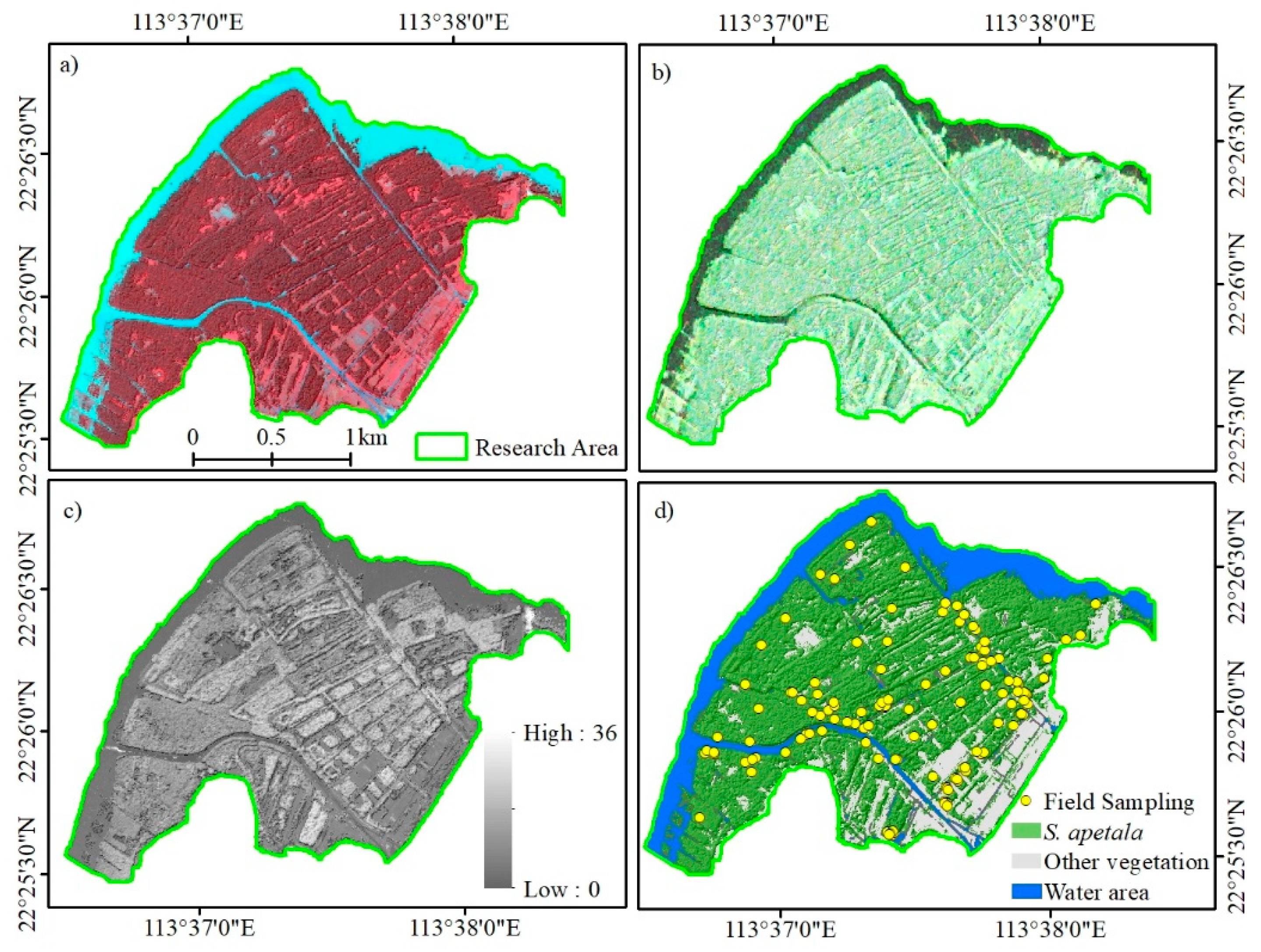
2.1. Study Area

This study was conducted in the mangrove nature reserve area of Guangdong Province in Dawei Bay of Qi’ao Island, in the Pearl River estuary of China (113°36′40″ E–113°39′15″ E, 22°23′40″ N–22°27′38″ N) [43,44]. It is a typical tropical and subtropical wetland ecosystem. The area of the reserve is 5103 ha, covering about 700 ha of mangrove forests: the largest contiguous area of artificially planted mangroves in China [6,45]. Mangrove forests are characterized by high spatial variability that represents a dynamic landscape. The mangrove forests planted in the study area were composed mainly of a fast-growing species, Sonneratia apetala (S. apetala), which was introduced from Bengal. They belong to the woody mangrove species, with features of high adaptability and seed production [46]. The heights of their trees usually increase by about 1.5 m during each of the first few years [47,48]. They were the tallest tree species in the study area, ranging from 2 m to 20 m, and the diameter at breast height (DBH) of older trees can be as large as 30 cm.
S. apetala has been artificially planted on the island since 1999 to control invasive species, (i.e., Spartina alterniflora) and reconstruct mangrove forests. S. apetala generally has an afforestation specification of 1–2 m × 1.5 m with high densities. The tree ages range from 1 year to 17 years with high biomass variability and complication. Its afforestation process runs seaward from land, which implies a gradient distribution of tree age and AGB. The mangrove plantations had extended throughout the study area, and S. apetala had become the dominant species, covering more than 80% of the mangrove forest.

2.2. Field Investigation

We conducted field investigations to obtain biomass samples from June to July in 2016. To ensure the availability of samples to build estimation models for the AGB, we collected 127 samples along almost all the accessible tidal creeks to account for the variation in the biomass of all stages of tree growth. The samples were located in the low-, middle-, and high-intertidal zones (Figure 1d). For each sample, we measured the height and diameter at breast height (DBH) of each tree and recorded data for trees within a 10 × 10 m quadrat. Tree height was measured by a handheld laser range finder (precision of 1 m; Trueyard SP-1500H, Trueyard Optical Instruments co.), and DBH higher than 5 cm was recorded by a breast diameter ruler at 1.3 m above the ground. To match the locations of the samples and overlaid images coordinates, the four vertices and center of each quadrat were recorded by a submeter-accurate GPS. The precise locations of the plots were recorded with the assistance of the GPS and high-resolution images (UAV images with 0.12 m spatial resolution). Details of the locations of the quadrats, such as distance to the shore, were identified in and marked on the images. Using the measured tree heights and DBHs during the field survey, we calculated the AGB of each mangrove tree using allometric equations [49], and computed the sum of the AGB of all trees within a quadrat, to represent the AGB of a sample.

2.3. Remote Sensing Data and Preprocessing Procedure

2.3.1. GF2 Optical Data
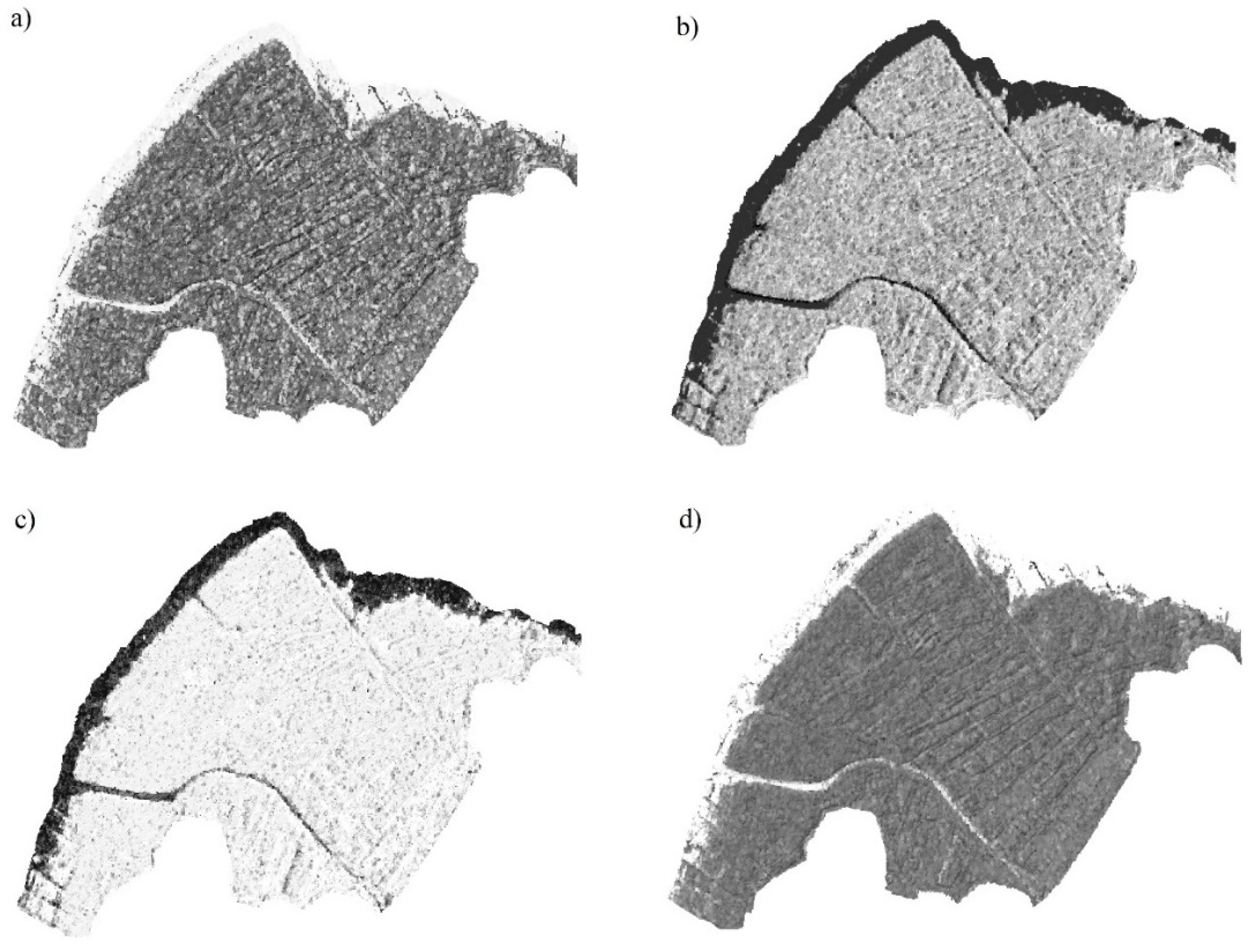
Gaofen-2 (GF-2) captures high-resolution images. It was launched by China National Space Administration (CNSA), Beijing, China, in August 2014. It has been applied to land monitoring, urban planning, and resource surveys [50]. GF-2 images have a panchromatic band (1-m resolution) and four multispectral bands (4-m resolution): red (R), green (G), blue (B), and near-infrared (NIR). We obtained GF-2 multispectral images on 15 February 2017 from Land Observation Satellite Data Service Platform (Figure 1a).
The pre-processing of the GF-2 images—including radiation calibration, atmospheric correction, and geometric correction—was carried out using the ENVI 5.4.1 software package. Atmospheric correction of the images was carried out using the fast line-of-sight atmospheric analysis of the spectral hypercubes (FLAASH) model with the ENVI module. The images were also geo-rectified to a 1:10,000 topographic map using ground control points, to ensure that the position error was smaller than 0.5 pixels.
After preprocessing, the images were used to calculate four vegetation indices (VIs)—difference vegetation index (DVI), ratio vegetation index (RVI), normalized difference vegetation index (NDVI) and soil-adjusted vegetation index (SAVI)—as input variables to estimate the AGB of the mangrove forest (Table 1).

2.3.2. GF3 SAR Data

The Gaofen-3 (GF-3), launched in August 2016, was developed by the China National Space Administration (CNSA), and is the first Chinese satellite that collects multi-polarized C-band SAR data. GF-3 images are the only radar images in the Chinese High-resolution Earth Observation System [55]. They have 12 imaging modes, ranging from single to dual and full polarization, with a resolution of 1 to 500 m and have a revisiting period of 3.5 days at most to the same point on Earth. Such characteristics render the GF-3 suitable for resource monitoring. We obtained fully polarimetric (FP) SAR data (HH, HV, VH, VV) from the Land Observation Satellite Data Service Platform on 5 August 2017, in the Quad-Polarization Stripmap 1 (QPS1) imaging mode at an azimuth resolution of 5.3 m, range resolution of 2.25 m, range of incidence angle of 29.63°, and in the single-look complex (SLC) format (Figure 1b and Table 2). Based on the original data, the image-related data were preprocessed to preserve phase and amplitude information in the complex images.
(1) Preprocessing of GF-3 images
FP SAR images contain speckle noise and geometric distortions that can have a significant negative impact on features of the polarization of the target objects. Thus, a preprocessing sequence consisting of data import, multi-look processing, adaptive filtering, radiometric calibration, and the geometric correction was applied to the GF-3 images using the SARscape 5.4.1 module embedded into the ENVI software. The steps of the preprocessing are as follows:
a) The metadata of the SAR images was imported to obtain the slant-range resolution and angle of incidence. The ground-range resolution was then calculated using the following:
R g r o u n d = R s l a n t sin ( θ )
where Rground represents ground-range resolution (4.5480 m), Rslant is the slant-range resolution (2.2484 m), and θ is the incidence angle (29.6281°).
b) The multi-look method was applied to de-speckle and re-sample the full-polarization GF-3 images. The GF-3 SAR images had a 1 × 1 multilook (azimuth × range), and were resampled to a regular grid with 5 × 5 m pixels in terms of azimuth and range resolution (5.30 × 2.25 m).
c) After the multi-look processing, the images were preprocessed using adaptive filters to reduce speckle and to enhance the edges and other features. We applied the refined Lee method of adaptive filtering by setting a 5 × 5 m filter window.
d) Radiometric calibration was carried out to convert the intensity values to the calibrated backscattering coefficient σo (dB) of the normalized radar using the following equation [56]:
σ ° = 10 × lg ( D N 2 ) + K
where DN represents the pixel values of the complex images, and K is the calibration constant. This equation referred to ALOS satellite processing. The radiometric calibration is still being explored to better process GF-3 SAR images. Previous studies used equation 2 to perform radiometric calibration, and demonstrated its utility and obtained satisfactory results [57,58]. Further study for radiometric calibration of Gaofen-3 images is needed.
e) Finally, the corrected backscatter map was generated from the backscattering coefficients to reduce the negative effect of the incidence angle on the radar’s backscatter. Geometric correction is then performed to match the positions of the ground control points selected in the GF2 images to corresponding points in a 1:10000 topographic map, with the positional error smaller than 0.5 pixels.
(2) Variables derived from GF-3 images
The preprocessed images were used to acquire HV/HH-, VH/HH-, HV/VV-, and VH/VV-polarized data, by calculating the ratio of the backscattering coefficients of different polarimetric channels.
The FP SAR data allow us to identify the scattering mechanisms of different types that can significantly improve the depiction of features of the target object. This was achieved by polarimetric decomposition techniques, to separate the received signals of the radar. Such analysis can help repose a simpler object susceptible to an easier physical interpretation as a combination of the scattering [59]. Coherent decomposition is used to measure the scattering matrix by the responses of coherent scatters [60]. The targets of coherent scatter are analyzed based on the Sinclair matrix (S) representing all polarimetric information. With linear horizontal (H) and vertical (V) polarizations, the Sinclair matrix can be expressed as follows:
S = [ s H H s H V s V H s V V ]
The Pauli and Krogager decomposition approaches were used to analyze the targets of coherent scatter based on the Sinclair matrix [61]. Both could be applied to a homogeneous distribution of mangrove species in the study area [62]. Pauli decomposition was used to extract features of the polarization of the objects by defining different polarization fundamental matrices representing various types of objects. Pauli’s polarimetric parameters were then decomposed into three elementary scattering mechanisms: odd-bounce scattering (P1), even-bounce scattering (P2), and volume scattering (P3). The Krogager decomposition aims to decompose the scattering matrix of a complex symmetric radar target into the physical interpretation of three components: sphere (KS1), diplane (KD3), and helix (KH2) [63].
The radar vegetation index (SAR-RVI), derived from FP SAR images, was used as a measure of the randomness of scattering from vegetation. It models the vegetation canopy as a collection of randomly oriented dipoles [64], and has yielded a good correlation between the SAR-RVI and the AGB. It was calculated by preprocessed FP data as follows [65]:
SAR-RVI = 8 × σ H V 2 × σ H V + σ H H + σ V V
where σHH, σHV, σVH, and σVV represent the backscattering coefficients of the polarimetric channels HH, HV, VH, and VV, respectively.
In this study, the 11 predictors derived from GF-3 SAR images—the four backscattering coefficients (HH, HV, VH, and VV) of the FP channels, three Pauli polarimetric parameters (P1, P2, and P3), three Krogager polarimetric parameters (KS1, KD3, and KH2), and the SAR-RVI—were used as input parameters to build and predict the AGB of mangrove forests. They can reflect the different properties of mangrove forests. The backscatter of HH is linked to both trunk and crown biomass, HV and VH return crown biomass, VV is dominated by branch biomass [66,67]. For the ratio of backscattering, they can potentially reduce topographic effects and forest structural effects, thereby increasing estimation accuracy [68]. The SAR-RVI reflects the canopy vegetation characteristics [64,69]. The Pauli decomposition can be used to separate the scattering matrix into simpler scattering responses related to single bouncing (e.g., canopy surface), double bouncing (e.g., trunk) and volume scattering (e.g., crown) [70,71]. The Krogager decomposition is related to surface, two, and three-sided corner reflectors [72]. The partial variables are shown in Figure 2.

2.3.3. UAV-Based DSM

DSM data were derived from a fixed-wing UAV with an onboard SONY NEX-5T camera and GPS/inertial measurement unit in 2016. The configuration of the UAV was set to an altitude of 400 m, 80% frontal overlap, and 60% side overlap. A total of 349 valid photographs were captured with geolocation and altitude embedded into the EXIF data. They were processed by the Agisoft PhotoScan Professional (64 bit) software. The DSM data were generated by overlapping photographs and the SfM photogrammetry algorithm and were exported at a resolution of 0.12 m (Figure 1c). A geometric correction was then executed by a 1:10,000 topographic map and ground control points.

2.3.4. Mangrove Classification Based on GF-2 and DSM Data

In this study, we just focus on the AGB estimation of mangrove plantation species, S. apetala. Their spatial distribution needed to be identified to map and predict AGB. The mangrove plantation (S. apetala), with a homogeneous distribution, was identified prior to AGB estimation. The plantation in the study area had distinctive traits, such as the tallest trees, from those of other mangrove species. The GF-2 and DSM data were integrated to extract characteristics of the mangrove plantation accurately. We collected over 700 samples for classification by field investigation. Half of them were used to build the classification models and the other half to validate them.
The multispectral and panchromatic bands of the GF-2 data were first fused by the pan-sharpening method. After image fusion, image objects were generated using a multi-resolution segmentation algorithm in eCognition Developer 9.0 software package. For each object, the mean values of the four bands and DSMs, Vis (DVI, RVI, NDVI, SAVI), and texture features (homogeneity, contrast, entropy, mean, and correlation) were calculated and used as input features. The random forest (RF) algorithm was used to train and build the classifier, using the input features and measured training samples. Finally, the RF models were used to predict maps of mangrove plantation. Compared with the measured test samples, the overall accuracy of the RF models for mangrove species classification was 86.14%.

2.4. Modeling and Accuracy Assessment of AGB Estimation

Models for the estimation of the biomass of the mangrove forest were developed using the random forest regression algorithm (RFR), which is an ensemble machine learning technique that consists of a large number (ntree) of decision trees grown by bootstraps of the original samples [73]. Each node of decision trees is separated by a random subset of input variables (mtry). The final results of the prediction are obtained by averaging the individual predictions of all regression trees [74]. The importance of all input variables was measured by out-of-bag (OOB) samples using the RF model and quantified by mean decrease in accuracy (MDA) [75]. Each variable’s MDA was calculated by the difference in OOB error between the original dataset and the dataset with randomly permutated variables. To reduce the randomness of the RF models, the mean importance values of the input variables were measured 50 times.
To integrate data from multiple sources, all variables derived from GF-2, GF-3, and DSM were resampled at a resolution of 4 m to correspond to the GF-2 images. The variables were used as input variables, and the measured AGB samples were used as output variables to build the RF models. The spatial distribution of the AGB across the study area was predicted and mapped by the built RF models. We employed iterated five-fold cross-validation by partitioning the AGB samples into five datasets, four of which were used for training and one for validation to ensure the stability, reliability, and generalization capability of the models. All five datasets were generated using stratified random sampling, which led them to represent the entire range of biomass values. The accuracies of the built models were assessed by the root-mean-square error (RMSE) and relative RMSE (RMSEr) calculated from the observed and predicted values of the AGB.
To qualify the effect of the input variables on the accuracy of estimation of the AGB, four experiments were conducted. RF models were built to this end by combining different types of variables. In experiment 1 (Expt. 1 for short), the model used eight variables derived from optical images of the GF-2, including the four bands, DVI, RVI, NDVI, and SAVI. In experiment 2 (Expt. 2), the model employed 15 variables derived from GF-3 SAR images: the four full polarizations (HH, HV, VV, and VH); the ratio of backscattering coefficients of different polarimetric channels (HV/HH, VH/HH, HV/VV, and VH/VV); Pauli decomposition (P1, P2, and P3); Krogager decomposition (KS1, KD3, and KH2); and the SAR-RVI. In experiment 3 (Expt. 3), the model used 23 variables through a combination of GF-2 optical and GF-3 SAR data. In experiment 4 (Expt. 4), the model used 24 variables by integrating GF2 optical, GF3 SAR, and UAV-based DSM data.

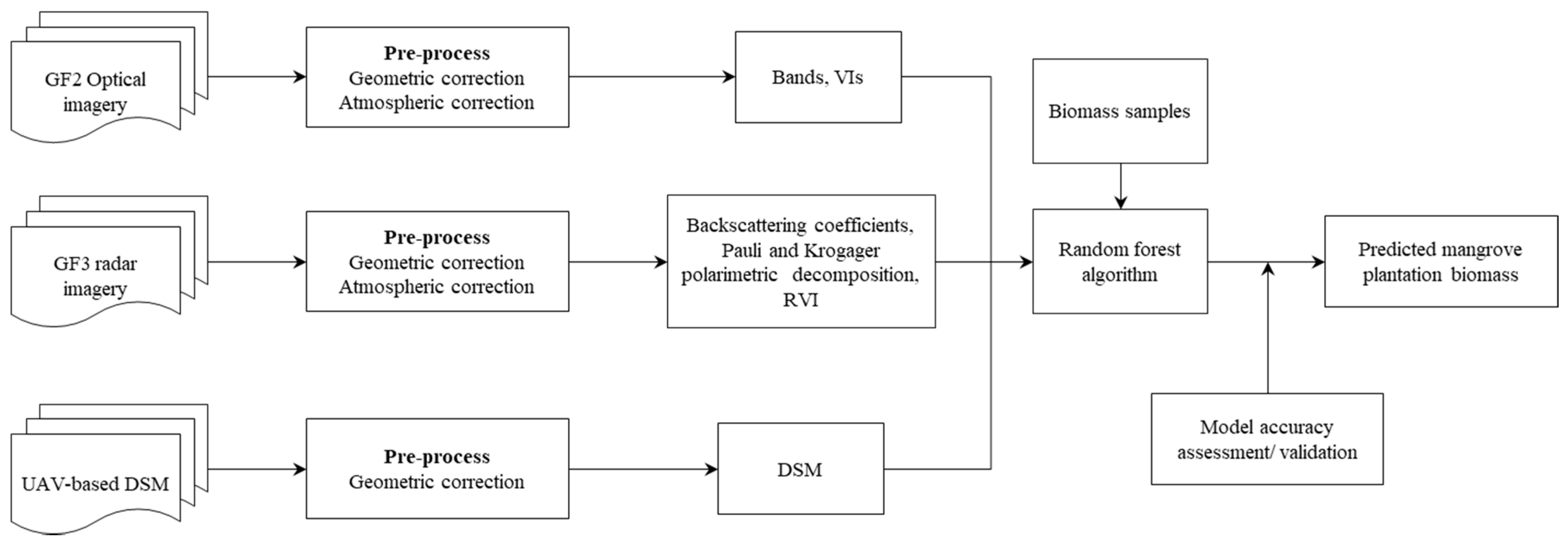
2.5. Workflow for Analyses

This study focuses on developing effective models of the AGB of a mangrove plantation based on images from multiple sources, including GF-2 optical, GF-3 SAR, and UAV-based DSM images. The models were built using a machine learning approach (i.e., random forest (RF)), and the input variables were derived from multiple datasets. The corresponding accuracies were examined to study the effect of the input variables on the monitoring of the AGB. Finally, the model with the highest accuracy was used to predict and map the spatial distribution of the AGB of mangrove plantations. The workflow is provided in Figure 3.

3. Results

3.1. AGB from Field Sampling

Field data of the mangrove plantation were collected a few times in the study area, and a total of 127 sampling units were obtained. The AGB was calculated by the allometric equation of the specific species. The plantation S. apetala had a density of 1623 trees per ha. The heights of the tree ranged from 2 to 20 m, with an average of 13.64 m. As it is a fast-growing species, the AGB of the mangrove plantation ranged from 90.65 to 237.74 t/ha, with an average of 159.70 t/ha, exhibiting a wide extent (43.88 t/ha of standard deviations), owing to their different ages. The field data revealed decreasing trends of AGB values in accordance with the sequence of growth from shore to sea.

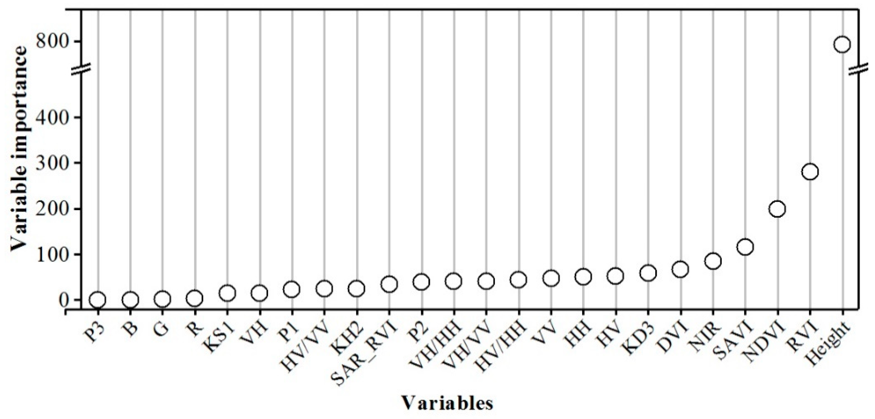
3.2. Importance of Input Variables for AGB Estimation

The importance of the input variables was quantified by the RF algorithm to evaluate the relationship between them and the AGB (Figure 4). The results showed that the most important variable was the UAV-based DSM, implying that it is key to the AGB estimation. The next most-important variables were the VIs (RVI, NDVI, etc.) derived from GF-2 optical images, followed by those (KD3, HV, etc.) derived from the GF-3 SAR images.

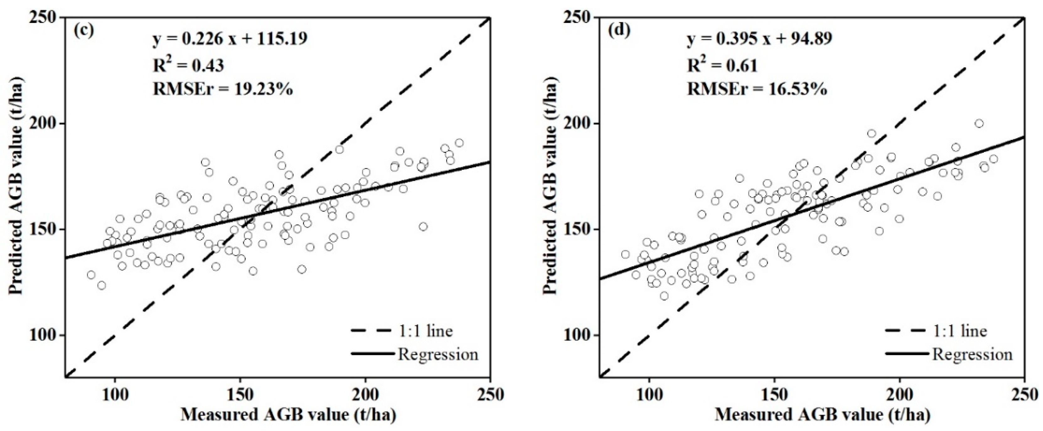
3.3. Results and Accuracy Assessment of AGB Model

The RF models were developed using the observed AGB as output variables and the variables derived from images from multiple sources as input variables. The RMSE and RMSEr were acquired by the observed and the predicted AGB values based on five-fold cross-validation. As shown in Table 3, the mean of the predicted AGB values in the four experiments was 156 t/ha, in line with the mean observed value. The model using input variables derived from the GF-3 SAR images yielded the lowest estimation accuracy of the AGB of mangroves, followed by the model that used the GF-2 optical images. The estimation accuracy of the model obtained through the integration of GF-2 and GF-3 images was better than the model that used either GF-2 or GF-3 data, with a reduction of 2.32% and 3.49% in RMSEr, respectively. The combination of GF-2, GF-3, and DSM data produced the highest accuracy (RMSE = 25.69 t/ha, RMSEr = 16.53%) of all models. A two-sided t-test revealed significant differences (p ≥ 0.95) in the predicted AGB values between models, using the combination of GF-2, GF-3, and DSM data, and those using only GF-2 or GF-3 images, but no significant difference (p < 0.95) was observed between the values obtained by models formed by a combination of GF-2, GF-3, and DSM data, and those obtained by models formed through the combination of GF-2 and GF-3 images.
Scatterplots of the predicted versus the measured AGB values are presented to show the accuracy of the models with different input variables using the RF algorithm and five-fold cross-validation in the study area. As shown in Figure 5, the predicted AGB values of all models were above the 1:1 line at lower values, indicating that AGB values of the mangrove plantation had been overestimated, but they were the opposite at higher values. The coefficient of determination (R2) of the model derived by integrating GF-2, GF-3, and UAV-based DSM data was 0.61, followed by the model obtained by a combination of GF-2 and GF-3 images. The other two models yielded lower R2 values.

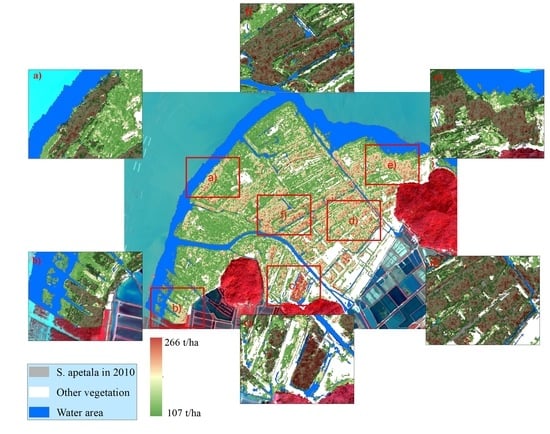
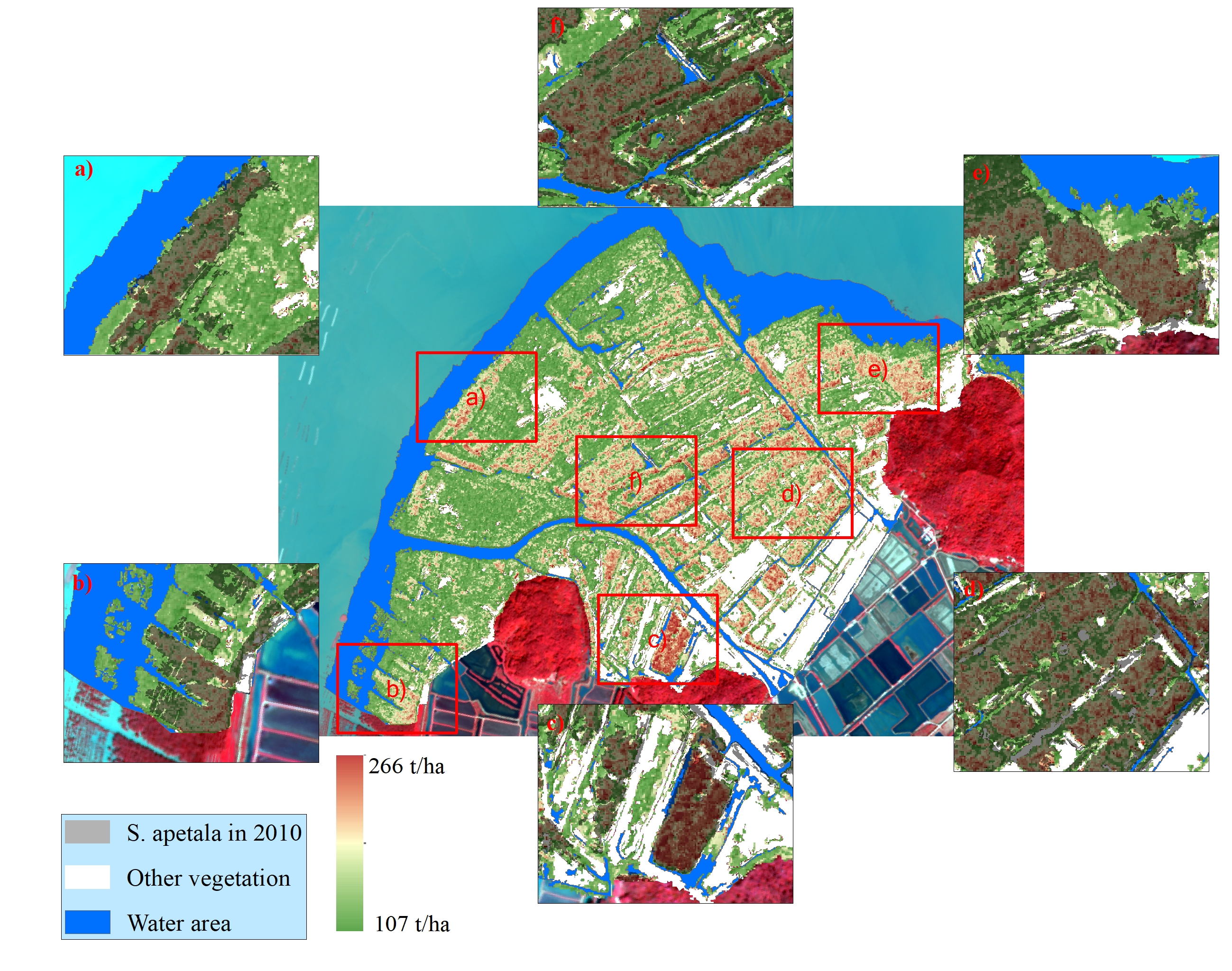
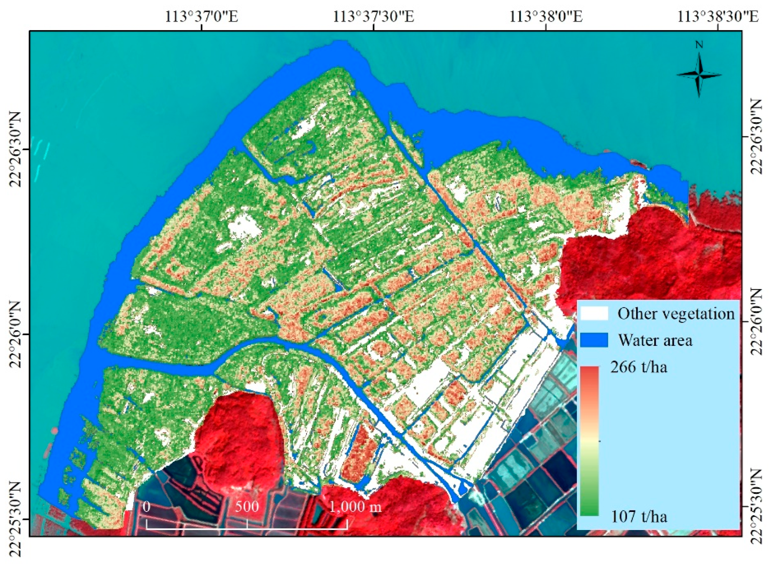
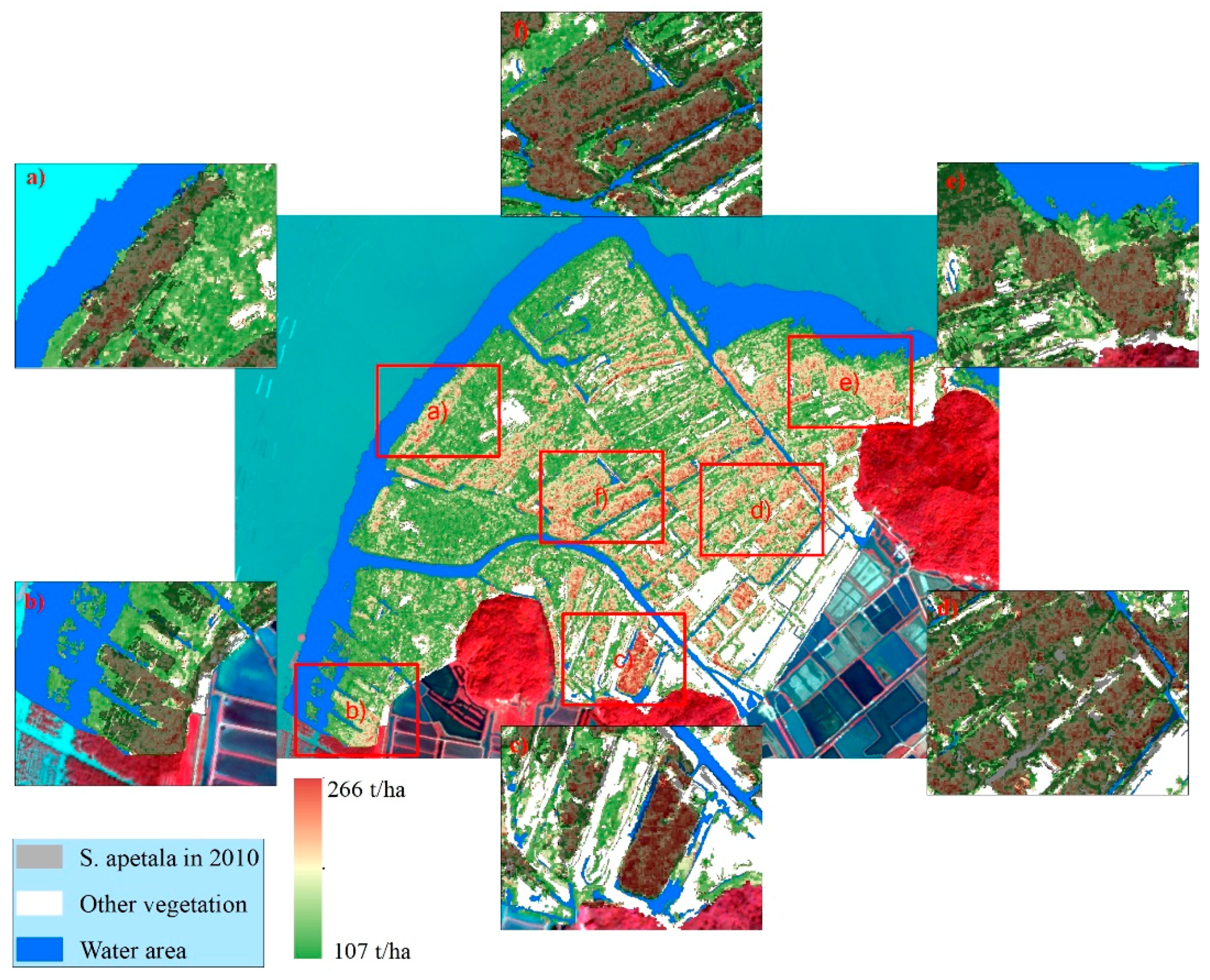
3.4. Mapping AGB of Mangrove Plantation

The model derived using a combination of GF-2, GF-3, and UAV-based DSM data produced the highest accuracy, and was used to map the spatial distribution of the AGB across the study area (Figure 6). The AGB map exhibited significant spatial variability, ranging from 106.163 t/ha to 266.162 t/ha, with an average of 137.89 t/ha. The AGB values of the species of mangrove in the southeast of the study area were higher than those in the west and northwest. The biomass decreased progressively from shore to sea, and trees near the shore had larger canopies and higher AGB values because they were older than those in other areas. Trees growing outside the forest edge and off the shore were younger and exhibited smaller biomass. The mangrove plantation map was consistent with the results of the field surveys, visual interpretation of remotely sensed images, and prior knowledge of Qi’ao Island.

4. Discussion

Estimating the AGB of forests based on satellite remote-sensing images remains challenging for tropical and subtropical mangrove forests, owing to various factors that interfere in the relationship between the AGB and the variables of images, such as the complex nature of their environments and complex forest structures [17]. The AGB of a forest has a close relationship, with its canopy-related information, structure, and height of trees, where single remote-sensing data cannot simultaneously provide this information [76]. Previous studies have investigated the combination of optical images (Landsat, SPOT, Sentinel-2, etc.) and SAR images (Sentinel-1, ALOS, etc.) to improve the accuracy of estimation of the AGB of forests [17,18]. The feasibility and applicability of data from the new GF-2 and GF-3 satellites from the Chinese civilian High-definition Earth Observation Satellite (HDEOS) program, launched in 2014 and 2016, respectively, by the China National Space Administration (CNSA), need to be tested.

4.1. Overall Performance of Random Forest Model

The objective of this study was to develop an accurate and robust biomass estimation of mangrove plantations. A random forest model was selected to establish non-linear relationships between the AGB and the input variables, because of its ease of use and prediction accuracy [43]. Previous studies already used machine-learning algorithms, such as support vector regression (SVR) or artificial neural network (ANN) for AGB estimation, which produces satisfactory results. Wang et al. (2016) investigated the applicability of RF, SVR, and ANN for remotely estimating wheat biomass, and the results indicated that the RF model produced more accurate estimates of wheat biomass than the SVR and ANN models at each stage [77].
A major advantage of RF is bootstrap sampling and variable sampling, in which the subset of all variables is randomly selected using the best split for each node of the standard regression tree. In these situations, The RF model can decrease the algorithm’s risk for overfitting and multicollinearity, due to relative insensitivity to variations in input variables, thereby improving generalization and robustness to predicted data. Therefore, some variables in this study are correlated. However, as demonstrated by Cutler et al., the RF model is not sensitive to collinearity, and has the ability to model complex and nonlinear interactions among predictor variables [78]. This is helpful, as it is commonly hard to determine which variables need to be removed when two or more variables correlate with each other [79]. Therefore, the RF algorithm provides a useful exploratory and predictive tool for estimating mangrove biomass.

4.2. Contribution of Input Variables to Measuring AGB of Mangrove Plantation

This study addressed the above issues using GF-2 optical and GF-3 data. The results indicated that the potential of the optical images and C-band FP SAR images for the AGB prediction of artificially planted mangroves were similar. The SAR-based results have been slightly weaker than the results with optical data, mainly due to weaker spatial resolution of the available SAR data in this study (5×5 m pixel resolution after multi-look method processing). On the other hand, the radiometric calibration referred to ALOS satellite processing using the SARscape, which may cause the errors of biomass estimation [57,58]. The advantages of SAR images are their multi-temporal acquisitions and independence of cloud cover, making the atmospheric correction of optical images more difficult [18].
The model of the AGB developed using a combination of GF-2 and GF-3 images yielded a higher estimation accuracy than those built using GF-2 or GF-3 images alone. This finding is consistent with previous studies, which have noted that integrating optical and SAR images can improve the accuracy of estimation of the AGB of forests, mainly because factors influencing biomass estimation, such as canopy-related information (canopy density, vegetation status) and forest structure, can be reflected by them [18,80].
However, optical or SAR images often incur saturation problems in canopies owing to dense vegetation, leading to the underestimation of biomass [81]. When considering variables of the DSM based on GF-2 and GF-3 images, the accuracy of the AGB model improved by 2.7% in terms of RMSEr. DSM data were also identified as the most important variable by the RF algorithm, because they were collected on a similar date with field measurements and can reflect the relative height of trees in a mangrove plantation, which is important for biomass estimation [42]. Tree height is usually computed from corresponding digital terrain models (DTM) subtracted from digital surface models (DSM). However, the DTM for dense mangrove forests is unavailable, due to the inability to penetrate their dense and complex canopy structures. The DTM is a stable constant for mangrove forests, because they mainly grow over even terrain [42]. The DSM can thus be considered to measure the relative heights of mangrove trees instead of the canopy height model (CHM). Previous studies have shown that the DSM derived from SfM and aerial photographs can solve the saturation problem and improve the estimation accuracy of biomass [82,83].
In this study, the P3, B, G, and R variables are least important (Figure 4). These variables with relatively low importance may be caused by the insensitivity to AGB estimation or be affected by multicollinearity. For example, the near-infrared (NIR) band of optical images is more widely used to estimate vegetation biomass content, because of its spectral reflection features in green vegetation, and visible (red, green, and blue) bands are usually used to emphasize vegetation health and classification, thus, they may be insensitive to AGB estimation. However, if the features have a correlation, it can be challenging to rank the importance of the features.

4.3. Spatial Distribution Patterns of AGB of Mangrove Plantation

As an initial effort for restoration and reforestation, the mangrove species S. apetala was introduced to the study area in 1999. As a result of its ability to spread, the artificial planting of S. apetala is becoming increasingly controversial as it may invade other mangrove ecosystems. The map of the AGB of the mangrove plantation derived here can provide baseline data for subsequent analyses and applications (e.g., carbon sequestration). The AGB values were predicted and mapped by a model that used GF-2 optical, GF-3 SAR, and UAV-based DSM data. The S. apetala afforestation process runs seaward from land, which implies a gradient distribution of AGB. The spatial distribution of the resulting AGB corresponded to the sequence of the mangrove plantation over time. To further verify the reliability of the model and understand the spatial distribution of the AGB, areas occupied by the mangrove plantation that had grown before 2011 were extracted by WorldView-2 images [43]. They exhibited significantly higher AGB values than the other areas, due to their age and fast growth. This is shown in Figure 7. The results thus indicate that the map of the AGB of the unevenly aged mangrove plantation showed a greater heterogeneity of AGB values.

4.4. Limitation and Sources of Errors

We found a reasonable relationship among GF-2 optical, GF-3 SAR images and, field measured AGB by using the RF algorithm. The combination of multi-source datasets (GF-2, GF-3 images, and DSM) yielded a higher estimation accuracy. However, there are some limitations and sources of errors from the AGB estimation using multi-source images, caused by position errors of geometric calibration, and the time difference of images and field measurements.
The errors of geometric calibration among multi-source images were unavoidable, though we used a geometric calibration to a 1:10,000 topographic map using ground control. The mismatch of the pixels derived from multi-source may cause the uncertainty of AGB estimation. Similarly, we got the AGB samples by field investigation, and the closest remotely sensed data available. The differences in time acquisitions may bring additional sources of errors in the AGB estimation, due to the fast-growing characteristic of the S. apetala. The study from Ren et al. (2010) suggested that AGB accumulation rates at the S. apetala plantations decreased with the stand ages [48]. The AGB accumulation rates were 20.3 t/ha from 4 to 5 years stand, 5.6 t/ha from 5 to 8 years stand, and 2.85 t/ha from 8 to 10 years stand, respectively. In our study area, most of the plantations have reached over 5 years stand [84], and previous study has demonstrated mean AGB accumulation of S. apetala over the study area to be 4.17 t/ha per year [85]. The average of observed values of this study is 155.4 t/ha, which may cause a 2.68% error of AGB—which is within the acceptable range—due to the different date between the field data and the images. Therefore, the inevitable difference of one year between the remote sensing images and in situ measurements can be deemed acceptable.

5. Conclusions

This study explored the potential of GF-2 optical, GF-3 SAR, and UAV-based DSM data for estimating the AGB of the mangrove plantation of Qi’ao Island in China. The AGB model generated using a combination of GF-2 and GF-3 images from the Chinese civilian HDEOS program yielded a higher accuracy than those of models using only one of these datasets, with a reduction of 2.32% and 3.49%, respectively, in RMSEr. When considering variables of the DSM derived from the UAV platform, the AGB model achieved the highest accuracy with a further reduction of 2.7% decrease in RMSEr. The DSM was the most important input variable for AGB estimation as it deals with saturation problems in optical and SAR images. The resulting AGB map agreed well with field surveys and the growing sequence of mangrove plantations. The results showed that accurate AGB models and spatial distribution maps of mangrove plantation can be obtained using the RF model, and images from multiple sources (GF-2 optical, GF-2 SAR, and UAV-based DSM data). The combination of these data provided canopy-related information, forest structures, and tree heights for AGB modeling.
The study focused on the integration of GF2 optical, GF3 SAR, and UAV data for estimating aboveground biomass in China’s largest artificially planted mangroves. The methodology can be used to produce accurate AGB models of mangrove forests, which can be difficult to obtain by field investigation. The AGB maps of S. apetala can help measure mangrove carbon sinks and provide baseline data for REDD+ programs, due to mangrove plantation. Future studies should further examine and improve AGB estimation uncertainty, such as accurate radiometric calibration and noise estimation of GF-3.

Author Contributions

Conceptualization, Y.Z., K.L. and L.L. conceived and designed the paper. Y.Z., K.L., J.C. and Z.D. conducted field study and data processing. Y.Z., K.L., L.L., S.W.M., Y.L. and Z.W. wrote and revised the manuscript. All authors have read and agreed to the published version of the manuscript.

Funding

This work is supported by Research Team Program of Natural Science Foundation of Guangdong Province, China (2014A030312010), China Postdoctoral Science Foundation (2018M633023), Postdoctoral International Training Program of Guangzhou City, Science and Technology Planning Project of Guangdong Province (2017A020217003), the Natural Science Foundation of Guangdong (2016A030313261 and 2016A030313188), and the National Science Foundation of China (Grant No. 41501368).

Conflicts of Interest

The authors declare no conflict of interest

References

  1. Kosoy, N.; Corbera, E. Payments for ecosystem services as commodity fetishism. Ecol. Econ. 2010, 69, 1228–1236. [Google Scholar] [CrossRef]
  2. Sani, D.A.; Hashim, M.; Hossain, M.S. Recent advancement on estimation of blue carbon biomass using satellite-based approach. Int. J. Remote Sens. 2019, 40, 7679–7715. [Google Scholar] [CrossRef]
  3. Laffoley, D.; Grimsditch, G.D. The Management of Natural Coastal Carbon Sinks; IUCN: Gland, Switzerland, 2009. [Google Scholar]
  4. Bouillon, S.; Borges, A.V.; Castañeda-Moya, E.; Diele, K.; Dittmar, T.; Duke, N.C.; Kristensen, E.; Lee, S.Y.; Marchand, C.; Middelburg, J.J. Mangrove production and carbon sinks: A revision of global budget estimates. Glob. Biogeochem. Cycles 2008, 22. [Google Scholar] [CrossRef] [Green Version]
  5. Jia, M.; Wang, Z.; Wang, C.; Mao, D.; Zhang, Y. A new vegetation index to detect periodically submerged Mangrove forest using single-tide sentinel-2 imagery. Remote Sens. 2019, 11, 2043. [Google Scholar] [CrossRef] [Green Version]
  6. Zhu, Y.; Liu, K.; Liu, L.; Wang, S.; Liu, H. Retrieval of Mangrove Aboveground Biomass at the Individual Species Level with WorldView-2 Images. Remote Sens. 2015, 7, 12192–12214. [Google Scholar] [CrossRef] [Green Version]
  7. Dou, Z.; Cui, L.; Li, J.; Zhu, Y.; Gao, C.; Pan, X.; Lei, Y.; Zhang, M.; Zhao, X.; Li, W. Hyperspectral Estimation of the Chlorophyll Content in Short-Term and Long-Term Restorations of Mangrove in Quanzhou Bay Estuary, China. Sustainability 2018, 10, 1127. [Google Scholar] [CrossRef] [Green Version]
  8. Giri, C.; Ochieng, E.; Tieszen, L.L.; Zhu, Z.; Singh, A.; Loveland, T.; Masek, J.; Duke, N. Status and distribution of mangrove forests of the world using earth observation satellite data. Glob. Ecol. Biogeogr. 2011, 20, 154–159. [Google Scholar] [CrossRef]
  9. Myint, S.W.; Giri, C.P.; Wang, L.; Zhu, Z.; Gillette, S.C. Identifying Mangrove Species and Their Surrounding Land Use and Land Cover Classes Using an Object-Oriented Approach with a Lacunarity Spatial Measure. GISci. Remote Sens. 2008, 45, 188–208. [Google Scholar] [CrossRef]
  10. Jia, M.M.; Wang, Z.M.; Zhang, Y.Z.; Mao, D.H.; Wang, C. Monitoring loss and recovery of mangrove forests during 42 years: The achievements of mangrove conservation in China. Int. J. Appl. Earth Obs. 2018, 73, 535–545. [Google Scholar] [CrossRef]
  11. Abdul Aziz, A.; Dargusch, P.; Phinn, S.; Ward, A. Using REDD+ to balance timber production with conservation objectives in a mangrove forest in Malaysia. Ecol. Econ. 2015, 120, 108–116. [Google Scholar] [CrossRef]
  12. Kankare, V.; Vastaranta, M.; Holopainen, M.; Räty, M.; Yu, X.; Hyyppä, J.; Hyyppä, H.; Alho, P.; Viitala, R. Retrieval of forest aboveground biomass and stem volume with airborne scanning LiDAR. Remote Sens. 2013, 5, 2257–2274. [Google Scholar] [CrossRef] [Green Version]
  13. Fatoyinbo, T.E.; Simard, M.; Washington-Allen, R.A.; Shugart, H.H. Landscape-scale extent, height, biomass, and carbon estimation of Mozambique’s mangrove forests with Landsat ETM+ and Shuttle Radar Topography Mission elevation data. J. Geophys. Res. Biogeosci. 2008, 113. [Google Scholar] [CrossRef]
  14. Pham, L.T.; Brabyn, L. Monitoring mangrove biomass change in Vietnam using SPOT images and an object-based approach combined with machine learning algorithms. ISPRS J. Photogramm. Remote Sens. 2017, 128, 86–97. [Google Scholar] [CrossRef]
  15. Sasmito, S.D.; Murdiyarso, D.; Wijaya, A.; Purbopuspito, J.; Okimoto, Y. Remote sensing technique to assess aboveground biomass dynamics of mangrove ecosystems area in Segara Anakan, Central Java, Indonesia. In Proceedings of the 34th Asian Conference on Remote Sensing 2013, ACRS 2013, Bali, Indonesia, 1 January 2013; pp. 4560–4565. [Google Scholar]
  16. Li, C.; Li, Y.; Li, M. Improving forest aboveground biomass (AGB) estimation by incorporating crown density and using landsat 8 OLI images of a subtropical forest in Western Hunan in Central China. Forests 2019, 10, 104. [Google Scholar] [CrossRef] [Green Version]
  17. Navarro, J.A.; Algeet, N.; Fernández-Landa, A.; Esteban, J.; Rodríguez-Noriega, P.; Guillén-Climent, M.L. Integration of UAV, Sentinel-1, and Sentinel-2 Data for Mangrove Plantation Aboveground Biomass Monitoring in Senegal. Remote Sens. 2019, 11, 77. [Google Scholar] [CrossRef] [Green Version]
  18. Vafaei, S.; Soosani, J.; Adeli, K.; Fadaei, H.; Naghavi, H.; Pham, T.; Tien Bui, D. Improving Accuracy Estimation of Forest Aboveground Biomass Based on Incorporation of ALOS-2 PALSAR-2 and Sentinel-2A Imagery and Machine Learning: A Case Study of the Hyrcanian Forest Area (Iran). Remote Sens. 2018, 10, 172. [Google Scholar] [CrossRef] [Green Version]
  19. Aslan, A.; Rahman, A.F.; Warren, M.W.; Robeson, S.M. Mapping spatial distribution and biomass of coastal wetland vegetation in Indonesian Papua by combining active and passive remotely sensed data. Remote Sens. Environ. 2016, 183, 65–81. [Google Scholar] [CrossRef]
  20. Jachowski, N.R.A.; Quak, M.S.Y.; Friess, D.A.; Duangnamon, D.; Webb, E.L.; Ziegler, A.D. Mangrove biomass estimation in Southwest Thailand using machine learning. Appl. Geogr. 2013, 45, 311–321. [Google Scholar] [CrossRef]
  21. Proisy, C.; Couteron, P.; Fromard, F. Predicting and mapping mangrove biomass from canopy grain analysis using Fourier-based textural ordination of IKONOS images. Remote Sens. Environ. 2007, 109, 379–392. [Google Scholar] [CrossRef]
  22. Le Maire, G.; Marsden, C.; Nouvellon, Y.; Grinand, C.; Hakamada, R.; Stape, J.-L.; Laclau, J.-P. MODIS NDVI time-series allow the monitoring of Eucalyptus plantation biomass. Remote Sens. Environ. 2011, 115, 2613–2625. [Google Scholar] [CrossRef]
  23. Pham, T.D.; Yoshino, K.; Bui, D.T. Biomass estimation of Sonneratia caseolaris (l.) Engler at a coastal area of Hai Phong city (Vietnam) using ALOS-2 PALSAR imagery and GIS-based multi-layer perceptron neural networks. GISci. Remote Sens. 2017, 54, 329–353. [Google Scholar] [CrossRef]
  24. Chadwick, J. Integrated LiDAR and IKONOS multispectral imagery for mapping mangrove distribution and physical properties. Int. J. Remote Sens. 2011, 32, 6765–6781. [Google Scholar] [CrossRef]
  25. Olagoke, A.; Proisy, C.; Féret, J.-B.; Blanchard, E.; Fromard, F.; Mehlig, U.; de Menezes, M.M.; Dos Santos, V.F.; Berger, U. Extended biomass allometric equations for large mangrove trees from terrestrial LiDAR data. Trees 2016, 30, 935–947. [Google Scholar] [CrossRef] [Green Version]
  26. Omar, H.; Misman, M.; Kassim, A. Synergetic of PALSAR-2 and Sentinel-1A SAR polarimetry for retrieving aboveground biomass in dipterocarp forest of Malaysia. Appl. Sci. 2017, 7, 675. [Google Scholar] [CrossRef] [Green Version]
  27. Wu, G.; Guo, Z.; Guo, J.; Zhu, Y. Estimation of mangrove wetland aboveground biomass based on remote sensing data: A review. J. South Agric. 2013, 44, 693–696. [Google Scholar]
  28. Cougo, M.; Souza-Filho, P.; Silva, A.; Fernandes, M.; Santos, J.; Abreu, M.; Nascimento, W.; Simard, M. Radarsat-2 backscattering for the modeling of biophysical parameters of regenerating mangrove forests. Remote Sens. 2015, 7, 17097–17112. [Google Scholar] [CrossRef] [Green Version]
  29. Kovacs, J.; Lu, X.; Flores-Verdugo, F.; Zhang, C.; de Santiago, F.F.; Jiao, X. Applications of ALOS PALSAR for monitoring biophysical parameters of a degraded black mangrove (Avicennia germinans) forest. ISPRS J. Photogramm. Remote Sens. 2013, 82, 102–111. [Google Scholar] [CrossRef]
  30. Lucas, R.; Lule, A.V.; Rodríguez, M.T.; Kamal, M.; Thomas, N.; Asbridge, E.; Kuenzer, C. Spatial ecology of mangrove forests: A remote sensing perspective. In Mangrove Ecosystems: A Global Biogeographic Perspective; Springer: Berlin/Heidelberg, Germany, 2017; pp. 87–112. [Google Scholar]
  31. Tsui, O.W.; Coops, N.C.; Wulder, M.A.; Marshall, P.L. Integrating airborne LiDAR and space-borne radar via multivariate kriging to estimate above-ground biomass. Remote Sens. Environ. 2013, 139, 340–352. [Google Scholar] [CrossRef]
  32. Haris, M.; Ashraf, M.; Ahsan, F.; Athar, A.; Malik, M. Analysis of SAR images speckle reduction techniques. In Proceedings of the 2018 International Conference on Computing, Mathematics and Engineering Technologies (iCoMET), Sukkur, Pakistan, 3–4 March 2018; pp. 1–7. [Google Scholar]
  33. Zhao, P.; Lu, D.; Wang, G.; Wu, C.; Huang, Y.; Yu, S. Examining spectral reflectance saturation in Landsat imagery and corresponding solutions to improve forest aboveground biomass estimation. Remote Sens. 2016, 8, 469. [Google Scholar] [CrossRef] [Green Version]
  34. Pham, T.D.; Yoshino, K.; Le, N.N.; Bui, D.T. Estimating aboveground biomass of a mangrove plantation on the Northern coast of Vietnam using machine learning techniques with an integration of ALOS-2 PALSAR-2 and Sentinel-2A data. Int. J. Remote Sens. 2018, 39, 7761–7788. [Google Scholar] [CrossRef]
  35. Shao, Z.; Zhang, L. Estimating forest aboveground biomass by combining optical and SAR data: A case study in Genhe, Inner Mongolia, China. Sensors 2016, 16, 834. [Google Scholar] [CrossRef] [Green Version]
  36. Hamdan, O.; Hasmadi, I.M.; Aziz, H.K.; Norizah, K.; Zulhaidi, M.H. L-band saturation level for aboveground biomass of dipterocarp forests in peninsular Malaysia. J. Trop. For. Sci. 2015, 27, 388–399. [Google Scholar]
  37. Fatoyinbo, T.E.; Simard, M. Height and biomass of mangroves in Africa from ICESat/GLAS and SRTM. Int. J. Remote Sens. 2013, 34, 668–681. [Google Scholar] [CrossRef]
  38. Fedrigo, M.; Newnham, G.J.; Coops, N.C.; Culvenor, D.S.; Bolton, D.K.; Nitschke, C.R. Predicting temperate forest stand types using only structural profiles from discrete return airborne lidar. ISPRS J. Photogramm. Remote Sens. 2018, 136, 106–119. [Google Scholar] [CrossRef]
  39. Fonstad, M.A.; Dietrich, J.T.; Courville, B.C.; Jensen, J.L.; Carbonneau, P.E. Topographic structure from motion: A new development in photogrammetric measurement. Earth Surf. Process. Landf. 2013, 38, 421–430. [Google Scholar] [CrossRef] [Green Version]
  40. Solberg, S.; Hansen, E.H.; Gobakken, T.; Næssset, E.; Zahabu, E. Biomass and InSAR height relationship in a dense tropical forest. Remote Sens. Environ. 2017, 192, 166–175. [Google Scholar] [CrossRef]
  41. Maimaitijiang, M.; Ghulam, A.; Sidike, P.; Hartling, S.; Maimaitiyiming, M.; Peterson, K.; Shavers, E.; Fishman, J.; Peterson, J.; Kadam, S.; et al. Unmanned Aerial System (UAS)-based phenotyping of soybean using multi-sensor data fusion and extreme learning machine. ISPRS J. Photogramm. Remote Sens. 2017, 134, 43–58. [Google Scholar] [CrossRef]
  42. Otero, V.; Van De Kerchove, R.; Satyanarayana, B.; Martínez-Espinosa, C.; Fisol, M.A.B.; Ibrahim, M.R.B.; Sulong, I.; Mohd-Lokman, H.; Lucas, R.; Dahdouh-Guebas, F. Managing mangrove forests from the sky: Forest inventory using field data and Unmanned Aerial Vehicle (UAV) imagery in the Matang Mangrove Forest Reserve, peninsular Malaysia. For. Ecol. Manag. 2018, 411, 35–45. [Google Scholar] [CrossRef]
  43. Zhu, Y.; Liu, K.; Liu, L.; Myint, S.; Wang, S.; Liu, H.; He, Z. Exploring the potential of worldview-2 red-edge band-based vegetation indices for estimation of mangrove leaf area index with machine learning algorithms. Remote Sens. 2017, 9, 1060. [Google Scholar] [CrossRef] [Green Version]
  44. Cao, J.; Leng, W.; Liu, K.; Liu, L.; He, Z.; Zhu, Y. Object-based mangrove species classification using unmanned aerial vehicle hyperspectral images and digital surface models. Remote Sens. 2018, 10, 89. [Google Scholar] [CrossRef] [Green Version]
  45. Liu, K.; Li, X.; Shi, X.; Wang, S.G. Monitoring mangrove forest changes using remote sensing and GIS data with decision-tree learning. Wetlands 2008, 28, 336–346. [Google Scholar] [CrossRef]
  46. Ren, H.; Lu, H.F.; Shen, W.J.; Huang, C.; Guo, Q.F.; Li, Z.A.; Jian, S.G. Sonneratia apetala Buch.Ham in the mangrove ecosystems of China: An invasive species or restoration species? Ecol. Eng. 2009, 35, 1243–1248. [Google Scholar] [CrossRef]
  47. Ren, H.; Jian, S.; Lu, H.; Zhang, Q.; Shen, W.; Han, W.; Yin, Z.; Guo, Q. Restoration of mangrove plantations and colonisation by native species in Leizhou bay, South China. Ecol. Res. 2008, 23, 401–407. [Google Scholar] [CrossRef] [Green Version]
  48. Ren, H.; Chen, H.; Han, W. Biomass accumulation and carbon storage of four different aged Sonneratia apetala plantations in Southern China. Plant Soil 2010, 327, 279–291. [Google Scholar] [CrossRef]
  49. Zan, q.j.; Wang, y.j.; Liao, b.w.; Zheng, d.z. Biomass and net productivity of Sonneratia apetala, S.caseolaris mangrove man-made forest. J. Wuhan Bot. Res. 2001, 19, 391–396. [Google Scholar]
  50. Wang, H.; Wang, C.; Wu, H. Using GF-2 imagery and the conditional random field model for urban forest cover mapping. Remote Sens. Lett. 2016, 7, 378–387. [Google Scholar] [CrossRef]
  51. Richardson, A.J.; Wiegand, C. Distinguishing vegetation from soil background information. Photogramm. Eng. Remote Sens. 1977, 43, 1541–1552. [Google Scholar]
  52. Tucker, C.J. Red and photographic infrared linear combinations for monitoring vegetation. Remote Sens. Environ. 1979, 8, 127–150. [Google Scholar] [CrossRef] [Green Version]
  53. Rouse, J.W., Jr.; Haas, R.; Schell, J.; Deering, D. Monitoring vegetation systems in the Great Plains with ERTS. In Proceedings of the Third Earth Resources Technology Satellite—1 Symposium: NASA SP-351, Washington, DC, USA, 10–14 December 1973; pp. 309–317. [Google Scholar]
  54. Huete, A.R. A soil-adjusted vegetation index (SAVI). Remote Sens. Environ. 1988, 25, 295–309. [Google Scholar] [CrossRef]
  55. Xu, L.; Zhang, H.; Wang, C.; Fu, Q. Classification of Chinese GaoFen-3 fully-polarimetric SAR images: Initial results. In Proceedings of the 2017 Progress in Electromagnetics Research Symposium—Fall (PIERS—FALL), Singapore, 19–22 November 2017; pp. 700–705. [Google Scholar]
  56. Shimada, M.; Isoguchi, O.; Tadono, T.; Isono, K. PALSAR Radiometric and Geometric Calibration. IEEE Trans. Geosci. Remote Sens. 2009, 47, 3915–3932. [Google Scholar] [CrossRef]
  57. Li, X.-M.; Zhang, T.; Huang, B.; Jia, T. Capabilities of Chinese Gaofen-3 synthetic aperture radar in selected topics for coastal and ocean observations. Remote Sens. 2018, 10, 1929. [Google Scholar] [CrossRef] [Green Version]
  58. Wang, H.; Li, H.; Lin, M.; Zhu, J.; Wang, J.; Li, W.; Cui, L. Calibration of the copolarized backscattering measurements from Gaofen-3 synthetic aperture radar wave mode imagery. IEEE J. Sel. Top. Appl. Earth Obs. Remote Sens. 2019, 12, 1748–1762. [Google Scholar] [CrossRef]
  59. Qi, Z.; Yeh, A.G.-O.; Li, X.; Lin, Z. A novel algorithm for land use and land cover classification using RADARSAT-2 polarimetric SAR data. Remote Sens. Environ. 2012, 118, 21–39. [Google Scholar] [CrossRef]
  60. Uhlmann, S.; Kiranyaz, S. Integrating Color Features in Polarimetric SAR Image Classification. IEEE Trans. Geosci. Remote Sens. 2014, 52, 2197–2216. [Google Scholar] [CrossRef]
  61. Huynen, J.R. Measurement of the target scattering matrix. Proc. IEEE 1965, 53, 936–946. [Google Scholar] [CrossRef]
  62. Yamaguchi, Y.; Moriyama, T.; Ishido, M.; Yamada, H. Four-component scattering model for polarimetric SAR image decomposition. IEEE Trans. Geosci. Remote Sens. 2005, 43, 1699–1706. [Google Scholar] [CrossRef]
  63. Krogager, E. New decomposition of the radar target scattering matrix. Electron. Lett. 1990, 26, 1525–1527. [Google Scholar] [CrossRef]
  64. Kim, Y.; Zyl, J.J.V. A Time-Series Approach to Estimate Soil Moisture Using Polarimetric Radar Data. IEEE Trans. Geosci. Remote Sens. 2009, 47, 2519–2527. [Google Scholar] [CrossRef]
  65. Wiseman, G.; McNairn, H.; Homayouni, S.; Shang, J. RADARSAT-2 polarimetric SAR response to crop biomass for agricultural production monitoring. IEEE J. Sel. Top. Appl. Earth Obs. Remote Sens. 2014, 7, 4461–4471. [Google Scholar] [CrossRef]
  66. Beaudoin, A.; Le Toan, T.; Goze, S.; Nezry, E.; Lopes, A.; Mougin, E.; Hsu, C.; Han, H.; Kong, J.; Shin, R. Retrieval of forest biomass from SAR data. Int. J. Remote Sens. 1994, 15, 2777–2796. [Google Scholar] [CrossRef]
  67. Ranson, K.; Sun, G. Mapping biomass of a northern forest using multifrequency SAR data. IEEE Trans. Geosci. Remote Sens. 1994, 32, 388–396. [Google Scholar] [CrossRef]
  68. Sarker, M.L.R.; Nichol, J.; Iz, H.B.; Ahmad, B.B.; Rahman, A.A. Forest biomass estimation using texture measurements of high-resolution dual-polarization C-band SAR data. IEEE Trans. Geosci. Remote Sens. 2012, 51, 3371–3384. [Google Scholar] [CrossRef]
  69. Gao, H.; Wang, C.; Wang, G.; Zhu, J.; Tang, Y.; Shen, P.; Zhu, Z. A crop classification method integrating GF-3 PolSAR and Sentinel-2A optical data in the Dongting Lake Basin. Sensors 2018, 18, 3139. [Google Scholar] [CrossRef] [PubMed] [Green Version]
  70. Tanase, M.A.; Panciera, R.; Lowell, K.; Tian, S.; Hacker, J.M.; Walker, J.P. Airborne multi-temporal L-band polarimetric SAR data for biomass estimation in semi-arid forests. Remote Sens. Environ. 2014, 145, 93–104. [Google Scholar] [CrossRef]
  71. Du, P.; Samat, A.; Gamba, P.; Xie, X. Polarimetric SAR image classification by boosted multiple-kernel extreme learning machines with polarimetric and spatial features. Int. J. Remote Sens. 2014, 35, 7978–7990. [Google Scholar] [CrossRef]
  72. Srikanth, P.; Ramana, K.; Deepika, U.; Chakravarthi, P.K.; Sai, M.S. Comparison of various polarimetric decomposition techniques for crop classification. J. Indian Soc. Remote Sens. 2016, 44, 635–642. [Google Scholar] [CrossRef]
  73. Breiman, L. Random forests. Mach. Learn. 2001, 45, 5–32. [Google Scholar] [CrossRef] [Green Version]
  74. Pal, M. Random forest classifier for remote sensing classification. Int. J. Remote Sens. 2005, 26, 217–222. [Google Scholar] [CrossRef]
  75. Liaw, A.; Wiener, M. Classification and regression by randomForest. R News 2002, 2, 18–22. [Google Scholar]
  76. Zhu, X.; Hou, Y.; Weng, Q.; Chen, L. Integrating UAV optical imagery and LiDAR data for assessing the spatial relationship between mangrove and inundation across a subtropical estuarine wetland. ISPRS J. Photogramm. Remote Sens. 2019, 149, 146–156. [Google Scholar] [CrossRef]
  77. Wang, L.a.; Zhou, X.; Zhu, X.; Dong, Z.; Guo, W. Estimation of biomass in wheat using random forest regression algorithm and remote sensing data. Crop J. 2016, 4, 212–219. [Google Scholar] [CrossRef] [Green Version]
  78. Cutler, D.R.; Edwards Jr, T.C.; Beard, K.H.; Cutler, A.; Hess, K.T.; Gibson, J.; Lawler, J.J. Random forests for classification in ecology. Ecology 2007, 88, 2783–2792. [Google Scholar] [CrossRef] [PubMed]
  79. Fukuda, S.; Yasunaga, E.; Nagle, M.; Yuge, K.; Sardsud, V.; Spreer, W.; Müller, J. Modelling the relationship between peel colour and the quality of fresh mango fruit using Random Forests. J. Food Eng. 2014, 131, 7–17. [Google Scholar] [CrossRef]
  80. Cutler, M.E.J.; Boyd, D.S.; Foody, G.M.; Vetrivel, A. Estimating tropical forest biomass with a combination of SAR image texture and Landsat TM data: An assessment of predictions between regions. ISPRS J. Photogramm. Remote Sens. 2012, 70, 66–77. [Google Scholar] [CrossRef] [Green Version]
  81. Mutanga, O.; Adam, E.; Cho, M.A. High density biomass estimation for wetland vegetation using worldview-2 imagery and random forest regression algorithm. Int. J. Appl. Earth Obs. 2012, 18, 399–406. [Google Scholar] [CrossRef]
  82. Luo, S.; Wang, C.; Xi, X.; Pan, F.; Peng, D.; Zou, J.; Nie, S.; Qin, H. Fusion of airborne LiDAR data and hyperspectral imagery for aboveground and belowground forest biomass estimation. Ecol. Indic. 2017, 73, 378–387. [Google Scholar] [CrossRef]
  83. Pena, J.M.; de Castro, A.I.; Torres-Sanchez, J.; Andujar, D.; San Martin, C.; Dorado, J.; Fernandez-Quintanilla, C.; Lopez-Granados, F. Estimating tree height and biomass of a poplar plantation with image-based UAV technology. AIMS Agric. Food 2018, 3, 313–326. [Google Scholar] [CrossRef]
  84. Liu, K.; Liu, L.; Liu, H.; Li, X.; Wang, S. Exploring the effects of biophysical parameters on the spatial pattern of rare cold damage to mangrove forests. Remote Sens. Environ. 2014, 150, 20–33. [Google Scholar] [CrossRef]
  85. Zhu, Y.; Liu, K.; Liu, L.; Myint, S.W.; Wang, S.; Cao, J.; Wu, Z. Estimating and Mapping Mangrove Biomass Dynamic Change Using WorldView-2 Images and Digital Surface Models. IEEE J. Sel. Top. Appl. Earth Obs. Remote Sens. 2020, 13, 2123–2134. [Google Scholar] [CrossRef]
Figure 1. Images of the study area. (a) Gaofen-2 (GF-2) images (bands 4, 3, 2 false-color combinations); (b) HH, HV, and VV color composition of Gaofen-3 (GF-3) images; (c) digital surface model (DSM) data derived from Unmanned Aerial Vehicle (UAV) images, and (d) spatial distribution of S. apetala and field sampling on Qi’ao Island.
Remotesensing 12 02039 g001
Figure 2. The partial variables derived from SAR images. (a) HV/HH, (b) P1 of Pauli decomposition, (c) KD3 of Krogager decomposition, and (d) radar vegetation index (SAR-RVI).
Remotesensing 12 02039 g002
Figure 3. Workflow for the measurement of the aboveground biomass of artificially planted mangroves by integrating images from GF-2, GF-3, and UAV-based DSM datasets.
Remotesensing 12 02039 g003
Figure 4. Importance of variables according to the random forest (RF) model.
Remotesensing 12 02039 g004
Figure 5. Scatter diagram of regression models detailing the linear regression, coefficient of determination (R²), and relative root-mean-square error (RMSEr) between field-measured aboveground biomass (AGB) and predicted AGB from (a) GF-2 optical images; (b) GF-3 SAR images; (c) a combination of GF-2 and GF-3; and (d) a combination of GF-2, GF-3, and DSM data.
Remotesensing 12 02039 g005aRemotesensing 12 02039 g005b
Figure 6. Spatial distribution of mangrove biomass.
Remotesensing 12 02039 g006
Figure 7. The predicted map of AGB values in 2016. (af) represented the partial enlarged detail of predicted mangrove AGB overlaid with the map of mangrove plantation from before 2011.
Remotesensing 12 02039 g007
Table 1. List of vegetation indices extracted from GF-2 optical data.
VegetationAcronymFormulaReference
Difference Vegetation IndexDVI D V I = N I R R [51]
Ratio Vegetation IndexRVI R V I = N I R R [52]
Normalized Difference Vegetation IndexNDVI N D V I = N I R R N I R + R [53]
Soil-Adjusted Vegetation IndexSAVI S A V I = [ N I R R N I R + R + L ] ( 1 + L ) [54]
Table 2. Characteristics of GF-3 synthetic aperture radar (SAR) images.
LevelImaging ModeFormatPolarization ModeIncidence AngleCoordinate
Level 1ASLCTIFF + RPCFull29.63°WGS-1984
Azimuth resolutionRange resolutionSizeCenter LongitudeCenter LatitudeTime
5.30 m2.25 m7435 × 7880113.7°22.4°5 August 2017
Table 3. The accuracy of mangrove biomass estimation based on different input variables.
Observed ValuesGF2GF3GF2 and GF3GF2, GF3, and DSM
Average (t/ha)155.43156.14156.54156.56156.23
Standard deviations (t/ha)37.7518.8114.7215.2519.08
Range (t/ha)90.65–237.74108.26–193.84120.91–191.14123.32–190.63118.33–200.72
RMSE (t/ha)/33.4935.3229.8925.69
RMSEr (%)/21.5522.7219.2316.53

