A Combined Use of TSVD and Tikhonov Regularization for Mass Flux Solution in Tibetan Plateau

1
College of Surveying and Geo-informatics, Tongji University, Shanghai 200092, China
2
Institute of Geodesy and Geoinformation, University of Bonn, Nussallee 17, 53115, Bonn, Germany
*
Author to whom correspondence should be addressed.
Remote Sens. 2020, 12(12), 2045; https://0-doi-org.brum.beds.ac.uk/10.3390/rs12122045
Submission received: 5 June 2020
/
Revised: 20 June 2020
/
Accepted: 23 June 2020
/
Published: 25 June 2020
Abstract
:Limited by the Gravity Recovery and Climate Experiment (GRACE) and GRACE Follow-On (GRACE-FO) measurement principle and sensors, the spatial resolution of mass flux solutions is about 2–3° in mid-latitudes at monthly intervals. To retrieve a mass flux solution in the Tibetan Plateau (TP) with better visual spatial resolution, we combined truncated singular value decomposition (TSVD) and Tikhonov regularization to solve for a mascon modeling. The monthly mass flux parameters resolved at 1° are smoothed to about 2° by truncating the eigen-spectrum of the normal equation (i.e., using the TSVD approach), and then Tikhonov regularization is applied to the truncated normal equation. As a result, the terms beyond the native resolution of GRACE/GRACE-FO data are truncated, and the errors in higher degree and order components are dampened by Tikhonov regularization. In terms of root mean squared errors, the improvements are 27.2% and 12.7% for the combined method over TSVD and Tikhonov regularization, respectively. We confirm a decreasing secular trend with −5.6 ± 4.2 Gt/year for the entire TP and provide maps with 1° resolution from April 2002 to April 2019, generated with the combined TSVD and Tikhonov regularization method.
1. Introduction
Since the launch of Gravity Recovery and Climate Experiment Follow-On (GRACE-FO) in May 2018 [1], the number of monthly products of time-variable gravity fields has grown, which provides the opportunity to further investigate large-scale secular and seasonal geophysical signals [2,3,4]. Known as the Third Pole, the Tibetan Plateau holds the largest number of glaciers, acting as an important contributor to major rivers in Asia, such as the Yangtze and the Ganges [5,6]. Due to the geographic complexity, remote sensing analyses, such as employing GRACE data, the digital elevation model (DEM) differencing approach, or converting height changes from laser altimetry (e.g., from Ice, Cloud, and Elevation Satellite, ICESat) to mass variations, are used in estimating the mass variation of the Tibetan Plateau (TP). For example, Brun et al. calculated the glacial mass loss at a trend of −16.3 ± 3.5 Gt/year between 2000 and 2016 in High Mountain Asia with a DEM [7] and Jacob et al. reported a less negative rate of −4 ± 20 Gt/year based on GRACE data [8]. The differences in mass trends that we find stress the need for a better understanding of the mass variations in the TP with high spatial resolution.
Due to the weak sensitivity of its observations in the east-west direction, measurement errors, and the ill-posed inversion problem, unconstrained GRACE-based spherical harmonic solutions show unreasonable north-south stripes [9]. Several post-processing techniques, such as applying Gaussian filters [10,11], decorrelation filters [12], and DDK filters [13,14], have been developed to constrain the errors in high degree and order. However, they tend to cause an attenuation of real geophysical signals [15]. Another option of recovering mass variations from GRACE data while avoiding the use of post-processing techniques is to use mass concentration approaches applied to GRACE inter-satellite range-rate measurements [16], or range-acceleration data [2,17], or spherical harmonic coefficients [8,18]. However, the normal equations that are formed within the mass concentration approach are typically ill-conditioned, and either truncated singular value decomposition (TSVD) or Tikhonov regularization is required to derive a stable solution. Moreover, the native spatial resolution of the mass flux solutions derived from GRACE data is about 2–3° (63,000 km2) at an error level of 2 cm in terms of equivalent water height (EWH) at monthly intervals [19].
It is well known that TSVD and Tikhonov regularization modify the eigen-spectrum of the normal equations in different ways, and combining the two methods adds one additional degree of freedom. More degrees of freedom for turning the normal equations are used in the multi-parameter regularization approach [20]. Although we cannot claim that the combination will automatically enable results superior to carefully tuned TSVD or Tikhonov regularization solutions, we hypothesize that it provides more flexibility when the gravity field is parameterized through mascons. The goal of the study is to derive an improved solution via the combined use of TSVD and Tikhonov regularization with respect to individual use of them: truncating the eigen-spectrum of the normal equation beyond the native spatial resolution of GRACE/GRACE-FO by TSVD, and then dampening the errors in higher degree and order components by Tikhonov regularization. The rest of this paper is organized as follows: Section 2 presents the combined TSVD and Tikhonov method after introducing the mascon modeling; Section 3 gives the details of total mass variations and spatial distribution of mass flux solution at 1° resolution in the TP and the conclusions are drawn in Section 4.
2. Data and Methods
2.1. GRACE Data
Since the launch of the GRACE mission in 2002, the GRACE Science Data System (SDS) institutions, namely, the Center for Space Research (CSR), the Jet Propulsion Laboratory (JPL), and the GeoForschungsZentrum (GFZ), have been updating gravity monthly solutions during release 01 to 06. Since the spatial, temporal, and spectral differences of these SDS products were shown to be within a certain scatter [21], they differ little among SDS products. Here we chose to employ the up-to-date CSR release 06 products [22] from April 2002 to April 2019 (172 months), including GRACE-FO data from June 2018 to April 2019. We follow the usual post-processing steps; since the GRACE monthly solutions refer to the center of mass, the offset between the center of mass and the center of the frame of the Earth, represented by the degree-1 coefficients of spherical harmonics [23], must be added back when the mass flux solutions are defined in the reference frame. We use degree-1 coefficients derived from satellite laser ranging (SLR) observations [24] to correct this offset. C20 and C30 terms, which are poorly observed by GRACE and GRACE-FO, in particular, with only a single accelerometer, are replaced with SLR observations by the technical note 14 (TN-14) document recommended by Loomis et al. [25].
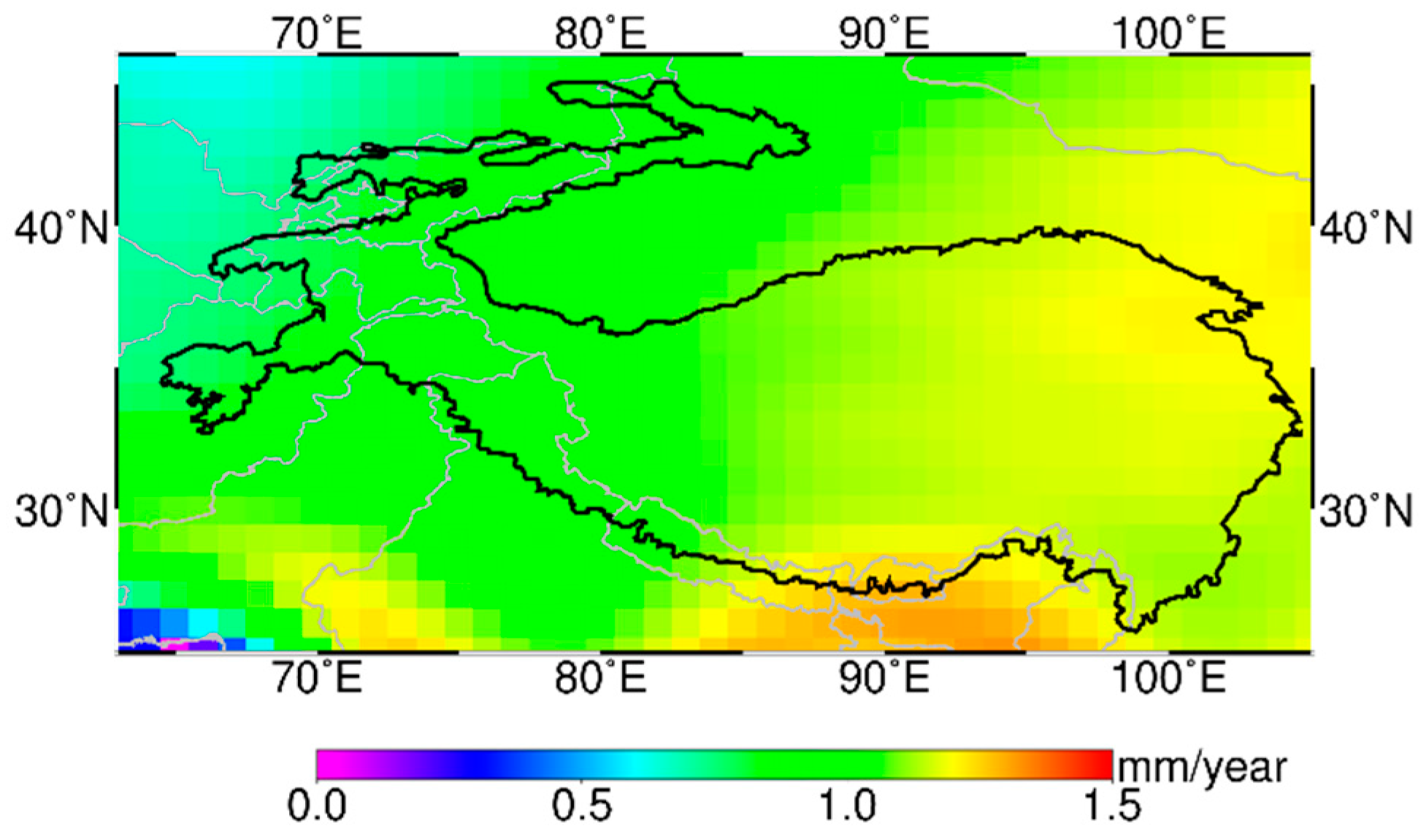
The response of the solid Earth to the glacial loading and unloading leads to glacial isostatic adjustment (GIA), and this signal should be removed from surface mass variations to enable an interpretation in terms of hydrology. We corrected our mass flux solution with the three-dimensional (3D) GIA model [26] and removed the GIA signal by 3.6 Gt/year from mass flux solution in the TP (Figure 1). With various ice sheet models and viscoelastic Earth models, other GIA models ranging from 0 mm/year to 2.5 mm/year account for mass variations of 0.2 Gt/year to 4.9 Gt/year in the TP, which indicate large uncertainties due to the complexity of the geodynamic process [27].
2.2. Mascon Modeling
In mascon approaches it is common to first transform the spherical harmonic coefficients into a set of pseudo-observables over the region of interest; typically, gravity disturbances at satellite altitude on a regular grid. When we account for the Earth’s elastic yielding, the radial gravity disturbance can be expressed in terms of fully normalized Stokes coefficients as follows [23],
where r, λ, and φ are the spherical coordinates of the pseudo observations (i.e., the radius (r = a + 500 km), longitude, and latitude, respectively); G indicates the gravitational constant; a is the mean radius of the Earth; l and m indicate the degree and order of the gravity field model; the maximum degree lmax is 60; (provided by Wahr et al. [11]) is the load Love number of degree l; Plm stands for the fully normalized associated Legendre functions; and are the Stokes coefficients after the mean gravity field is removed.
According to Newton’s law of gravity, assuming n pseudo observations at satellite attitude caused by t mass-points in the study area, the total radial gravitational disturbance at each location j is as follows [18],
where (j = 1,2,…,t) is the unknown mass variations to be estimated and is the spherical distance.
Together with Equations (1) and (2), the radial gravitational disturbance in the pseudo observation points at satellite altitude connects the spherical harmonic coefficients and the mass variation due to the ground mass-points, and we reformulated the observation equation here as
where y is an n-vector of pseudo observations of the radial gravitational disturbance calculated by spherical harmonic coefficients; A is an n × t design matrix (n > t) and denotes an overdetermined system of the equation; x is a t-vector of unknown ground mass-points to be estimated (i.e., ); e denotes the n-vector of random errors with zero mean and variance of unit weight . Via the law of error propagation, the weight matrix P is computed with P = (BDBT)−1, in which D is the covariance matrix from the CSR release 06 products; B is the coefficient matrix of projecting the spherical harmonics to the pseudo observation vector with its ith row elements corresponding to spherical harmonics andwhich are written as [28],
where is the spherical coordinate of the ith pseudo observation; and are the column numbers corresponding to spherical harmonics and, respectively. According to Ran et al. [29], introducing the weight matrix can improve the quality of estimated mass variations. Tikhonov regularization, with the L-curve method applied to choose the regularization parameter, is widely used in GRACE-derived regional and global mascon solutions [18,30].
Within our study area of 63°E-105°E, 25°N-46°N, we constructed a mascon grid at ground level, at 1° resolution with 946 mascons (Figure 1). In the figure, the center of each mascon (1° × 1°) stands for the coordinate of the corresponding ground mascon to be estimated. The mass flux solution for the entire TP consists of the individual mass variations of each mascon inside the boundary of the TP (black line in Figure 1). The pseudo observations of radial gravitational disturbance cover an area of 60°E-108°E, 22°N-49°N of 0.8° resolution and 1° resolution, respectively.
2.3. Combined Use of TSVD and Tikhonov Regularization
To recover the solution x, we applied the least-squares adjustment to minimize the square sum of e. The design matrix A (n × t) can be expressed by singular value decomposition (SVD) as
in which the columns of U = [ u1, u2, …, un] are the left singular vectors of A; the diagonal matrix S = diag[s1, s2, …, st] is the singular value of A; the columns of V = [v1, v2, …, vt] are the right singular vectors of A. The least-squares solution is,
As the index increases, the singular value of A increases as well and small perturbations in the observations can cause significant perturbations in the solution. Due to the sampling and geometry of pseudo observation, we found a condition number for the design matrix A of 6.9·1017 (with the geodesic grid of 1° × 1°), indicating an ill-conditioned normal equation N = ATPA. There are two regularization methods presented: TSVD and Tikhonov regularization. By eliminating small singular values, the TSVD solution xk is in the form of [31],
where 1 < k < t. If the truncation parameter k is chosen too large, the condition number of A remains large; however, a small k value leads to losing a large part of the signals. Tikhonov regularization is commonly applied to stabilize ill-posed problems, it is well-known that the solution minimizes the cost function
where indicates the regularization parameter ( > 0) and R is the regularization matrix. The solution to Equation (9) is expressed as,
which shows that Tikhonov regularization dampens every component of the design matrix.
Here we construct a new TSVD and Tikhonov regularization by applying Tikhonov regularization to the truncated normal equation. As the regularization matrix R is chosen as an identity matrix I and the design matrix A is truncated to the first k singular values, the solution is,
Consisting of the variance-covariance matrix of and the bias correction of both Tikhonov regularization and the truncated part [32,33], the corresponding mean squared error (MSE) matrix is,
in which is the true value, and . The variance matrix of is . The and correspond to bias impacts of Tikhonov regularization and TSVD, respectively. For more details, please refer to [32,33]. To estimate the unknown , the following equation is introduced [34],
in which is the estimation of the error vector. Since the true value remains unknown, we replaced it with the estimation by the combined method.
Comparing Equation (10) with Equation (11), it is obvious that this combined Tikhonov regularization adds a small regularization parameter to the truncated ( only. The choice of the truncated number k controls the amount of useful information derived from the normal equation and the Tikhonov regularization further dampens the errors of higher degree and order.
When considering the location of the inflection point of the eigenvalue curve for the case of 1° resolution, we selected the truncation parameter k as 270 (about 2° resolution) for the combined method; we then applied Tikhonov regularization to the truncated normal equation and derived the optimal regularization parameter based on the criterion of minimizing the traced MSE (for details, see [33,34]); finally, we calculated the mass flux solution with Equation (11). Other methods to determine the regularization parameter such as the discrepancy principle [35], the generalized cross-validation method [36], or the L-curve criterion [18,30] could be investigated.
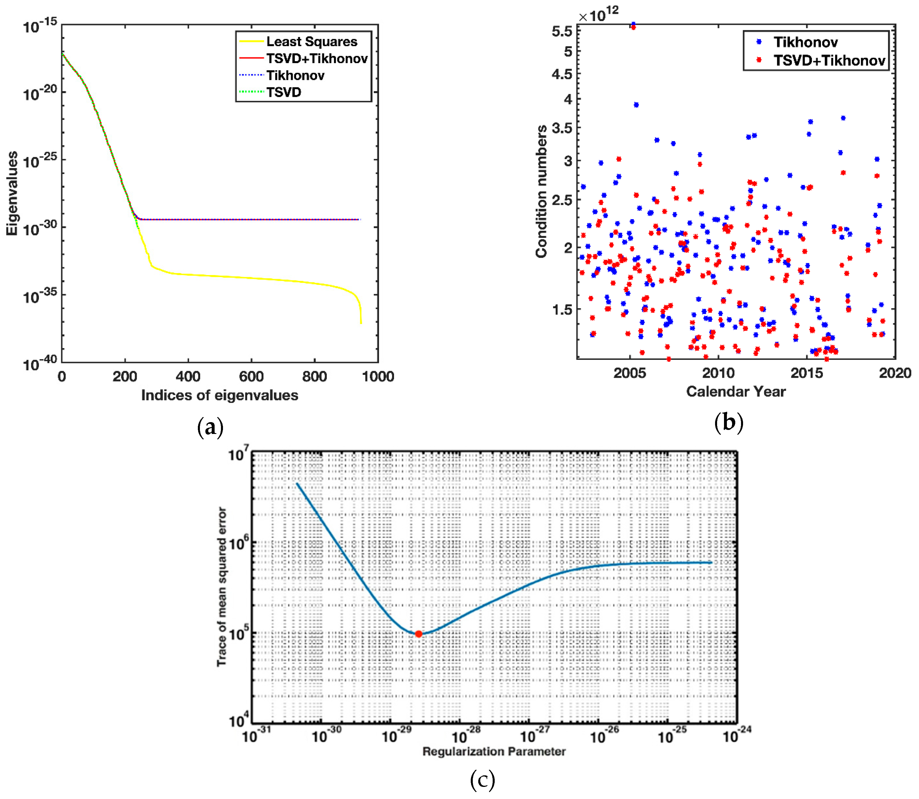
Figure 2a shows the eigenvalues of the normal equation with the 1° resolution with different methods in January 2004. It should be noted that the choice of regularization parameter and truncation value may bias the mass variations derived from the combined method, TSVD, or Tikhonov regularization. To compare the combined solution with other solutions, we did not truncate the normal equation with Tikhonov regularization only (Figure 2a, blue dotted line) and derived the optimal regularization parameter based on the criterion of minimizing the traced MSE. Note that the regularization parameters of the combined method and Tikhonov regularization are separately calculated for each month. The truncating parameter k of TSVD solutions is chosen according to the MSE criterion in each month [30]. We further compared the condition numbers by the combined method, and Tikhonov regularization, respectively in Figure 2b. The condition numbers by the combined methods were reduced slightly more compared to those by Tikhonov regularization during 2002 to 2019. Figure 2c presents how traced MSE of the combined method varies with the regularization parameter in January 2004. The regularization parameter of 1.6 × 10⁻²⁹ is selected by the minimum traced MSE.
Limited by the GRACE data, the spatial resolution of the solution is about 2°. Therefore all 1° grids are overparameterized; due to rounding error, the eigenvalues lower than 10−33 drop very slowly, and the correspondent eigenvectors form linearly dependent parameters. Truncating them to about a 2° resolution is better than direct parameterizing with 2° grids, since the combinations with larger eigenvalues are left. However, if we truncate more terms to get a stable solution, we may lose the signals corresponding to small eigenvalues. The terms for the eigenvalues larger than 10−33 are corresponding to the spatial resolution of GRACE data; Tikhonov regularization is therefore used to derive a stable solution.
2.4. Leakage Correction
The leakage errors in GRACE observations increase proportionally with the strength of the signal source and attenuate quickly with the increasing distance between the source and the mass points. Similar to other studies [28], we expanded the study area by 3°, covering the area of 60°E-108°E, 22°N-49°N, and calculated these additional mass variations outside the study area with mascon modeling as well. To eliminate the leakage error, we removed the radial gravitational disturbance derived from these nearby additional mass variations from our pseudo observations.
3. Results and Discussion
3.1. MSE Roots
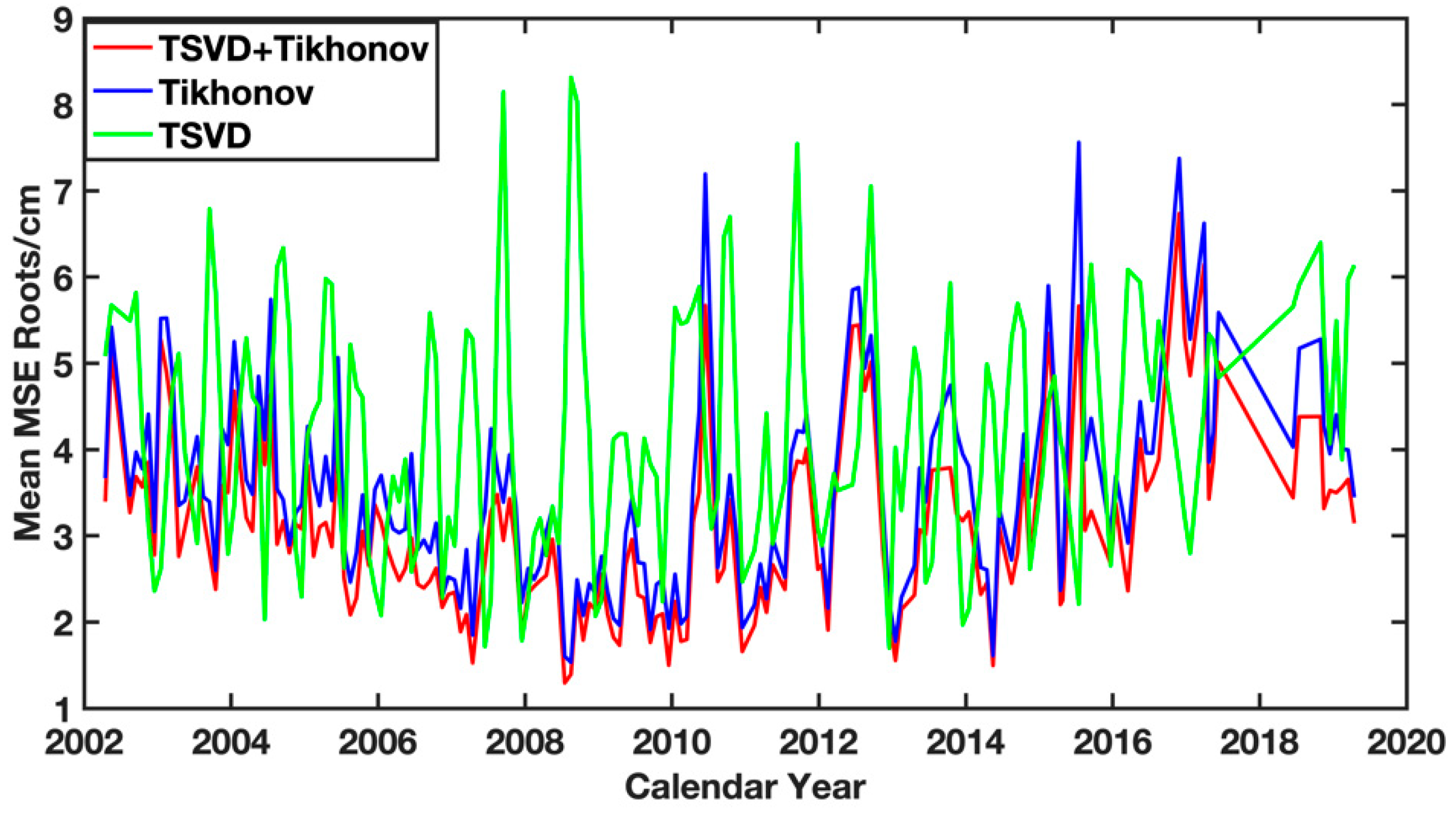
Here we introduced MSE, which is one of the most common measures to describe how methods perform in parameter estimation. Estimators (i.e., mascons in our case) with a smaller MSE, indicate that they are expected to have a closer distance to the true value. To compare the performance of each method in the parameter space, we calculated the MSE roots of 946 mascons in the TP using the combined method with Equation (12), those by TSVD according to Xu [32], and those by Tikhonov regularization according to Shen and colleagues [33]. Figure 3 shows the MSE roots in EWH (cm) of all mascons for each month. Except for a few months, the combined method has a better performance than Tikhonov regularization. The maximum MSE roots of 946 mascons were successfully reduced from 8.31 cm in the case of TSVD to 6.74 cm in the case of the combined method. The maximum MSE root by Tikhonov regularization is equal to 7.56 cm. The MSE roots of 3.08 cm by the combined method is smaller than those of 4.23 cm and 3.53 cm by TSVD and Tikhonov regularization, respectively (Table 1). In other words, the improvements are 27.2% and 12.7% for the combined method over TSVD and Tikhonov regularization.
3.2. Total Mass Variations
As expected, the time series of mass flux solution in the TP (i.e., within the black boundary in Figure 1) from April 2002 to April 2019 exhibited strong annual changes with a decreasing secular trend at a rate of −5.6 ± 4.2 Gt/year, −7.9 ± 3.9 Gt/year, −6.8 ± 5.2 Gt/year, and −8.6 ± 5.8 Gt/year with combined TSVD and Tikhonov regularization, TSVD only, Tikhonov regularization only, and P4M6 + 400 km Gaussian filtering [10,11,12] applying to mass points exactly those used in the combined method, respectively (Figure 4). Note that the TSVD solution suffers unrealistic south-north strips (see Figure 5d), indicating that using TSVD alone is not suitable to recover mass flux solution in the TP.
To investigate the secular trend and the seasonal mass variations, we established a fitting function to estimate the linear rate, (semi-) annual variations, as well as to remove a 161-day S2 alias that would remove an error due to incorrect modeling of the S2-tide, as follows,
where, A1, A2, A3, , , stand for the annual, semi-annual, and 161-day amplitudes and phases; t is the time tag in years; b is bias parameter; is the residuals. We realize that Equation (14) represents a mathematical model that enables an unbiased trend estimate, rather than a tool for assessing solution errors in the presence of real geophysical signals which do not necessarily follow this model. However, we argue that (1) it is indeed our primary aim to derive the mass trends, and (2) several modeling studies have confirmed that a trend plus (semi-) annual model describes snow accumulation, groundwater, and surface water change in the TP region quite well [37,38].
The similarity of the annual phase retrieved by all methods in Table 2 suggests that the mass storage of the Tibetan Plateau reaches a maximum in September, likely related to the large amount of precipitation in the TP between June and September which is brought by the southwest monsoon of the Indian Ocean [39,40]. Assume for the moment the fitting curve represents the true signal, we further derive an estimate for the root mean squared error (RMSE), the standard deviation of the residuals, and root mean squared (RMS) ratio defined as,
where RMS(fitting curve) refers to the latitude weighted RMS of the fitting curve; RMS(residuals) stands for RMS of residuals . The RMSE of the combined method is 1.9 cm, close to the RMSE of filtering, while that of the Tikhonov regularization is 2.2 cm (Table 2). The RMS ratio of 1.21 by the combined method is higher than those of 0.45, 0.78, and 1.16 by TSVD, Tikhonov regularization, and filtering, respectively, indicating that the combined method can retrieve annual and semi-annual signals at a higher confidence level. The improvements of the combined method relative to the Tikhonov regularization is 14% for RMSE, and 55% for RMS ratio.
When evaluated over the same period, the secular trend of total mass variations in the TP that we find with the combined method at 1° resolution is among the range of previous studies with different datasets (Table 3). The use of GeoForschungsZentrum (GFZ) release 06 data agrees with the results of the Center for Space Research (CSR) release 06 within 5%.
3.3. Mass Variations Distribution
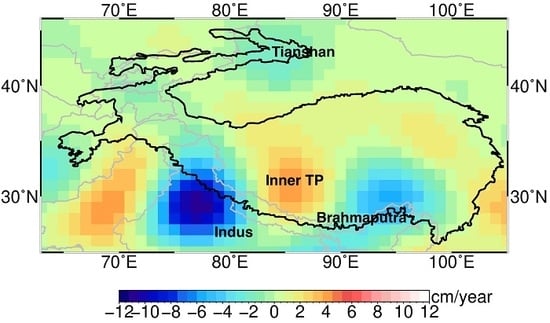
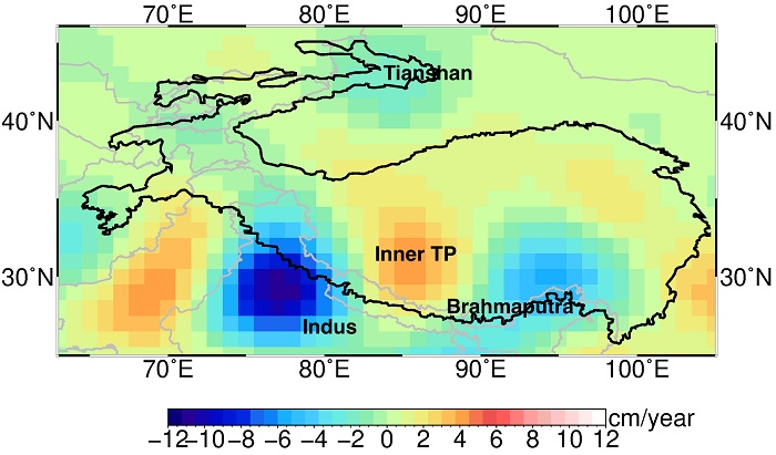
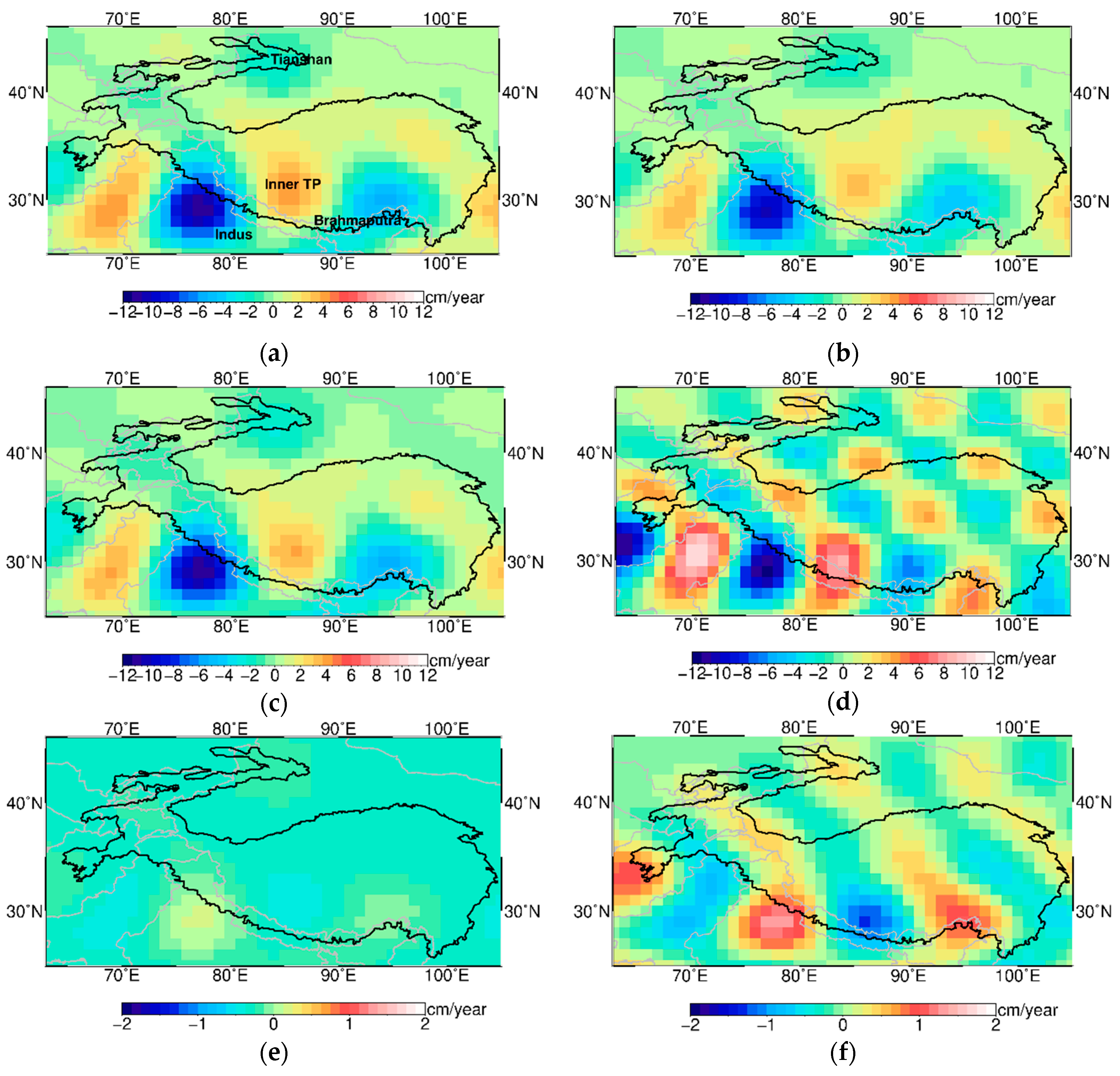
Figure 5 presents the spatial distribution of the secular trend, derived from the mass variations in TP: with the combined method, with the Tikhonov regularization, with P4M6 + 400 km Gaussian filter, with TSVD, with the filter minus those of the combined method, and with the Tikhonov regularization minus those of the combined method, respectively. The filtering results show signals relatively similar with the combined method; however, the TSVD-only method still exhibits significant south-north stripes. The trend map in Figure 5a–c shows the mass accumulation in the Inner TP at a maximum trend of 2.4 cm/year with the combined method. Two other significant signal sources are the Indus Basin located in North India and the Brahmaputra Basin located in the central and eastern Himalayas. The minimum secular trend from the mass flux solution derived from the combined method is found at −11.2 cm/year in the Indus Basin and −5.4 cm/year in the Brahmaputra Basin, while with Tikhonov regularization these trends remain as −8.9 cm/year and −4.2 cm/year, respectively. We speculate that in addition to the dampening by Tikhonov regularization, the relatively weaker signals could also be blamed by the low spatial resolution because a larger mass point covers more area and the mass variations in a large area will be smoothed if the strong signal is averaged together with weak ones in the same mass point. Note that the trend map is arranged from −2 to 2 cm in Figure 5e,f. Figure 5e shows the trends of the filtering solution minus those of the combined method, indicating that the result of the combined method presents no stripe pattern, just like the two-step filtering technique which is designed to remove the south-north stripes. Figure 5f gives the trends of the Tikhonov only method minus those of the combined method, showing south-north stripes. Since Figure 5e shows no evident south-north stripes, it is the result of Tikhonov regularization that contains stripe patterns.
The geophysical processes causing mass variations are complicated in the TP. The strong mass loss signal in north India is likely caused by the anthropogenic groundwater depletion, confirmed by groundwater-level monitoring data [41]. Global Positioning System observes long-term uplift rates as 0.5–0.7 cm/year in the TP, which might be isostatically compensated by an increasing mass deficiency at depth [42]. Gardner et al. [43] suggested rapid thinning rates of mountain glaciers in different sub-regions based on glacier elevation variations. The recharge pathway of the melt water remains unclear, and tends to sink into the ground, whose local storage capacity is limited due to permafrost [8].
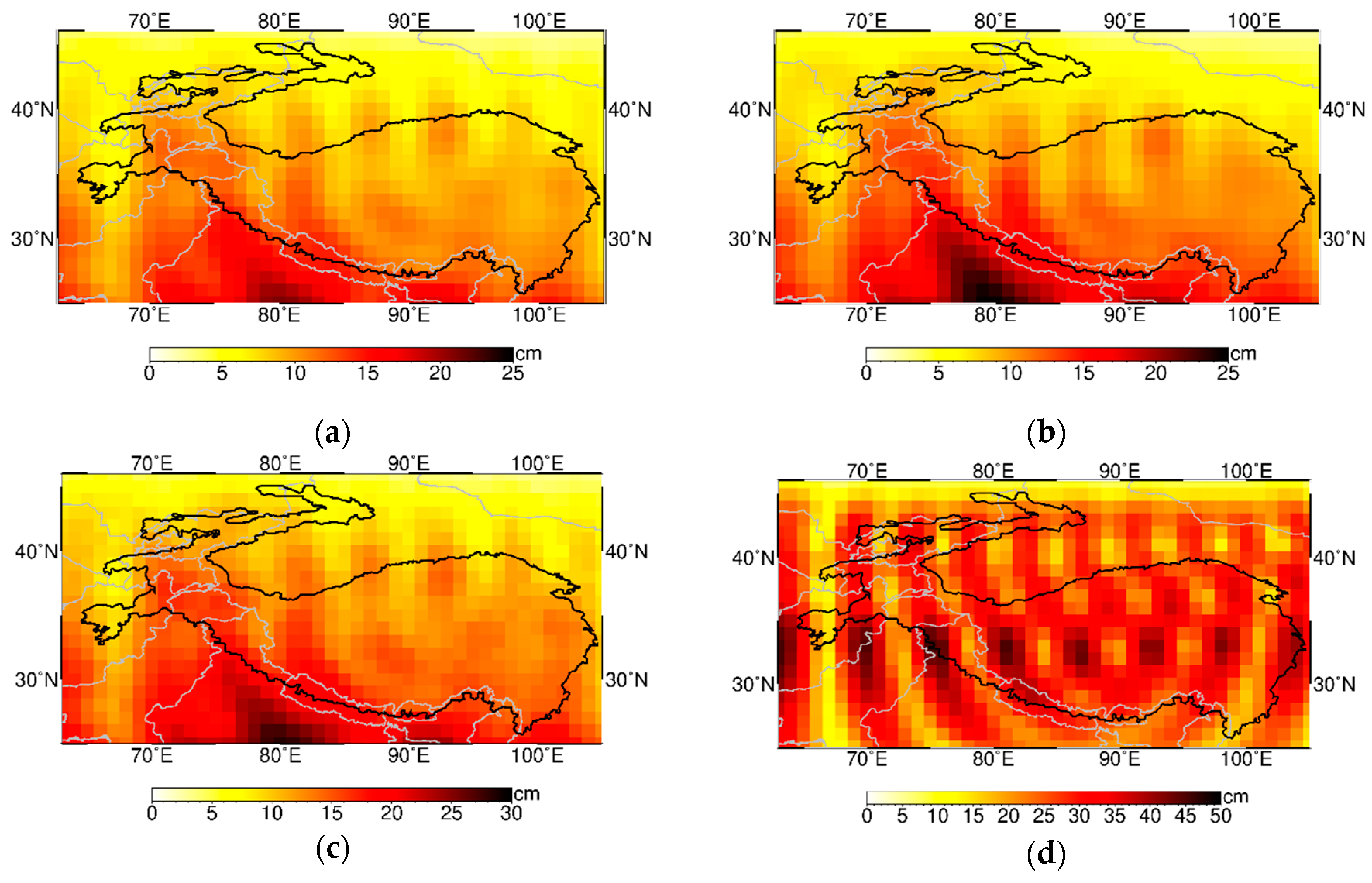
We then visualized the RMSE of each mass point in the TP to compare with those from the Tikhonov regularization, and from the filtering results (Figure 6). Note that the RMSE map is arranged from 0–30 cm and 0–50 cm in Figure 6c,d, respectively. The latitude weighed RMSE of the TP with the combined method was the smallest among the three methods (9.6 cm vs. 10.4 cm for Tikhonov, 12.2 cm for filtering, and 23.0 cm for TSVD), which is consistent with the improved RMSE and RMS ratio derived from the total mass variations. The largest difference of the RMSE is located in the southeast of the Indus Basin, reaching 22.9 cm from the combined method, 25.3 cm from the Tikhonov regularization, and 29.7 cm when using the filtering method. Along the Karakoram Mountains and the Himalayas Mountains, the larger RMSE indicates that the Tikhonov regularization and the filtering methods perform worse in retrieving secular and seasonal signals than the combined method.
4. Summary
We introduced a combined TSVD and Tikhonov regularization method to retrieve mass flux solutions at 1° resolution in the TP. This combined method truncates the terms beyond the native resolution of GRACE/GRACE-FO data and dampens the errors in higher degree and order components by Tikhonov regularization. Of course, the number of degrees of freedom in the truncated normal equation is approximately equal to those directly parameterized as 2°. The improvements for the combined method over TSVD and Tikhonov regularization are 27.2% and 12.7% in terms of MSE roots from 2002 to 2019. Furthermore, using TSVD or Tikhonov regularization alone leaves corresponding mass flux solutions in the TP with unrealistic south-north stripes, while the result of the combined method shows no evidence of stripes.
Author Contributions
Conceptualization, methodology, and supervision, Y.S.; original draft preparation, T.C.; revision, J.K.; data, Q.C. All authors have read and agreed to the published version of the manuscript.
Funding
This research was funded by the National Key R&D Program of China (2017YFA0603103), the National Natural Science Foundation of China (41731069,41974002), Chinese Scholarship Council (201706260151), as well as partially supported by the Alexander von Humboldt Foundation in Germany (awarded to Q.C.).
Conflicts of Interest
The authors declare no conflicts of interest.
References
- Flechtner, F.; Neumayer, K.-H.; Dahle, C.; Dobslaw, H.; Fagiolini, E.; Raimondo, J.-C.; Güntner, A. What can be expected from the GRACE-FO laser ranging interferometer for earth science applications? Surv. Geophys. 2016, 37, 453–470. [Google Scholar] [CrossRef] [Green Version]
- Luthcke, S.B.; Sabaka, T.J.; Loomis, B.D.; Arendt, A.A.; McCarthy, J.J.; Camp, J. Antarctica, Greenland and Gulf of Alaska land-ice evolution from an iterated GRACE global mascon solution. J. Glaciol. 2013, 59, 613–631. [Google Scholar] [CrossRef]
- Rignot, E.; Velicogna, I.; van den Broeke, M.R.; Monaghan, A.; Lenaerts, J.T.M. Acceleration of the contribution of the Greenland and Antarctic ice sheets to sea level rise: Acceleration of ice sheet loss. Geophys. Res. Lett. 2011, 38, L05503. [Google Scholar] [CrossRef] [Green Version]
- Chambers, D.P. Observing seasonal steric sea level variations with GRACE and satellite altimetry. J. Geophys. Res. 2006, 111. [Google Scholar] [CrossRef]
- Qiu, J. China: The third pole. Nature 2008, 454, 393–396. [Google Scholar] [CrossRef] [PubMed] [Green Version]
- Krause, P.; Biskop, S.; Helmschrot, J.; Flügel, W.-A.; Kang, S.; Gao, T. Hydrological system analysis and modelling of the Nam Co basin in Tibet. Adv. Geosci. 2010, 27, 29–36. [Google Scholar] [CrossRef] [Green Version]
- Brun, F.; Berthier, E.; Wagnon, P.; Kääb, A.; Treichler, D. A spatially resolved estimate of High Mountain Asia glacier mass balances, 2000–2016. Nat. Geosci. 2017, 10, 668–673. [Google Scholar] [CrossRef]
- Jacob, T.; Wahr, J.; Pfeffer, W.T.; Swenson, S. Recent contributions of glaciers and ice caps to sea level rise. Nature 2012, 482, 514–518. [Google Scholar] [CrossRef]
- Tapley, B.D.; Schutz, B.E.; Born, G.H. Statistical Orbit Determination; Elsevier Academic Press: Amsterdam, The Netherlands; Boston, MA, USA, 2004; ISBN 978-0-12-683630-1. [Google Scholar]
- Jekeli, C. Alternative Methods to Smooth the Earth’s Gravity Field; Report 327 of Geodetic Science and Surveying; Ohio Ohio State University: Columbus, OH, USA, 1981. [Google Scholar]
- Wahr, J.; Molenaar, M.; Bryan, F. Time variability of the Earth’s gravity field: Hydrological and oceanic effects and their possible detection using GRACE. J. Geophys. Res. Solid Earth 1998, 103, 30205–30229. [Google Scholar] [CrossRef]
- Swenson, S.; Wahr, J. Post-processing removal of correlated errors in GRACE data. Geophys. Res. Lett. 2006, 33. [Google Scholar] [CrossRef]
- Kusche, J. Approximate decorrelation and non-isotropic smoothing of time-variable GRACE-type gravity field models. J. Geod. 2007, 81, 733–749. [Google Scholar] [CrossRef] [Green Version]
- Kusche, J.; Schmidt, R.; Petrovic, S.; Rietbroek, R. Decorrelated GRACE time-variable gravity solutions by GFZ, and their validation using a hydrological model. J. Geod. 2009, 83, 903–913. [Google Scholar] [CrossRef] [Green Version]
- Tapley, B.D.; Watkins, M.M.; Flechtner, F.; Reigber, C.; Bettadpur, S.; Rodell, M.; Sasgen, I.; Famiglietti, J.S.; Landerer, F.W.; Chambers, D.P.; et al. Contributions of GRACE to understanding climate change. Nat. Clim. Chang. 2019, 9, 358–369. [Google Scholar] [CrossRef] [PubMed]
- Watkins, M.M.; Wiese, D.N.; Yuan, D.-N.; Boening, C.; Landerer, F.W. Improved methods for observing Earth’s time variable mass distribution with GRACE using spherical cap mascons: Improved Gravity Observations from GRACE. J. Geophys. Res. Solid Earth 2015, 120, 2648–2671. [Google Scholar] [CrossRef]
- Sabaka, T.J.; Rowlands, D.D.; Luthcke, S.B.; Boy, J.-P. Improving global mass flux solutions from Gravity Recovery and Climate Experiment (GRACE) through forward modeling and continuous time correlation. J. Geophys. Res. 2010, 115. [Google Scholar] [CrossRef]
- Baur, O.; Sneeuw, N. Assessing Greenland ice mass loss by means of point-mass modeling: A viable methodology. J. Geod. 2011, 85, 607–615. [Google Scholar] [CrossRef]
- Vishwakarma, B.D.; Devaraju, B.; Sneeuw, N. What is the spatial resolution of grace satellite products for hydrology? Remote Sens. 2018, 10, 852. [Google Scholar] [CrossRef] [Green Version]
- Eicker, A.; Schall, J.; Kusche, J. Regional gravity modelling from spaceborne data: Case studies with GOCE. Geophys. J. Int. 2014, 196, 1431–1440. [Google Scholar] [CrossRef] [Green Version]
- Sakumura, C.; Bettadpur, S.; Bruinsma, S. Ensemble prediction and intercomparison analysis of GRACE time-variable gravity field models. Geophys. Res. Lett. 2014, 41, 1389–1397. [Google Scholar] [CrossRef]
- University Of Texas Center For Space Research (UTCSR). GRACE Static Field Geopotential Coefficients CSR Release 6.0 2018. Available online: https://podaac.jpl.nasa.gov/dataset/GRACE_GSM_L2_GRAV_CSR_RL06 (accessed on 24 August 2019). [CrossRef]
- Hofmann-Wellenhof, B.; Moritz, H. Physical Geodesy, 2nd corrected ed.; Springer: Wien, Austria; New York, NY, USA, 2006; ISBN 978-3-211-33544-4. [Google Scholar]
- Cheng, M.; Tapley, B.D.; Ries, J.C. Deceleration in the Earth’s oblateness: J2 VARIATIONS. J. Geophys. Res. Solid Earth 2013, 118, 740–747. [Google Scholar] [CrossRef]
- Loomis, B.D.; Rachlin, K.E.; Wiese, D.N.; Landerer, F.W.; Luthcke, S.B. Replacing GRACE/GRACE-FO with satellite laser ranging: Impacts on Antarctic ice sheet mass change. Geophys. Res. Lett. 2020, 47. [Google Scholar] [CrossRef]
- Wahr, J.; Zhong, S. Computations of the viscoelastic response of a 3-D compressible Earth to surface loading: An application to Glacial Isostatic Adjustment in Antarctica and Canada. Geophys. J. Int. 2013, 192, 557–572. [Google Scholar] [CrossRef]
- Zhang, T.Y.; Jin, S.G. Estimate of glacial isostatic adjustment uplift rate in the Tibetan Plateau from GRACE and GIA models. J. Geodyn. 2013, 72, 59–66. [Google Scholar] [CrossRef]
- Chen, T.; Shen, Y.; Chen, Q. Mass flux solution in the Tibetan Plateau using mascon modeling. Remote Sens 2016, 8, 439. [Google Scholar] [CrossRef] [Green Version]
- Ran, J.; Ditmar, P.; Klees, R.; Farahani, H.H. Statistically optimal estimation of Greenland Ice Sheet mass variations from GRACE monthly solutions using an improved mascon approach. J. Geod. 2017. [Google Scholar] [CrossRef] [PubMed] [Green Version]
- Save, H.V. Using Regularization for Error Reduction in GRACE Gravity Estimation. Ph.D. Thesis, The University of Texas at Austin, Austin, TX, USA, 2009. [Google Scholar]
- Hansen, P.C. Truncated singular value decomposition solutions to discrete Ill-posed problems with Ill-determined numerical rank. SIAM J. Sci. Stat. Comput. 1990, 11, 503–518. [Google Scholar] [CrossRef]
- Xu, P. Truncated SVD methods for discrete linear ill-posed problems. Geophys. J. Int. 1998, 135, 505–514. [Google Scholar] [CrossRef]
- Shen, Y.; Xu, P.; Li, B. Bias-corrected regularized solution to inverse ill-posed models. J. Geod. 2012, 86, 597–608. [Google Scholar] [CrossRef]
- Xu, P.; Shen, Y.; Fukuda, Y.; Liu, Y. Variance component estimation in linear inverse Ill-posed models. J. Geod. 2006, 80, 69–81. [Google Scholar] [CrossRef]
- Reichel, L.; Shyshkov, A. A new zero-finder for Tikhonov regularization. BIT Numer. Math. 2008, 48, 627–643. [Google Scholar] [CrossRef]
- Kusche, J.; Klees, R. Regularization of gravity field estimation from satellite gravity gradients. J. Geod. 2002, 76, 359–368. [Google Scholar] [CrossRef]
- Yi, S.; Sun, W. Evaluation of glacier changes in high-mountain Asia based on 10 year GRACE RL05 models: Evaluation of glacier changes. J. Geophys. Res. Solid Earth 2014, 119, 2504–2517. [Google Scholar] [CrossRef]
- Pan, Y.; Shen, W.-B.; Hwang, C.; Liao, C.; Zhang, T.; Zhang, G. Seasonal mass changes and crustal vertical deformations constrained by GPS and GRACE in Northeastern Tibet. Sensors 2016, 16, 1211. [Google Scholar] [CrossRef] [PubMed] [Green Version]
- Zou, F.; Tenzer, R.; Jin, S. Water storage variations in Tibet from GRACE, ICESat, and hydrological data. Remote Sens. 2019, 11, 1103. [Google Scholar] [CrossRef] [Green Version]
- Jiang, W.; Yuan, P.; Chen, H.; Cai, J.; Li, Z.; Chao, N.; Sneeuw, N. Annual variations of monsoon and drought detected by GPS: A case study in Yunnan, China. Sci. Rep. 2017, 7. [Google Scholar] [CrossRef] [PubMed]
- Long, D.; Chen, X.; Scanlon, B.R.; Wada, Y.; Hong, Y.; Singh, V.P.; Chen, Y.; Wang, C.; Han, Z.; Yang, W. Have GRACE satellites overestimated groundwater depletion in the Northwest India Aquifer? Sci. Rep. 2016, 6. [Google Scholar] [CrossRef] [PubMed]
- Bettinelli, P.; Avouac, J.-P.; Flouzat, M.; Jouanne, F.; Bollinger, L.; Willis, P.; Chitrakar, G.R. Plate motion of india and interseismic strain in the Nepal Himalaya from GPS and DORIS measurements. J. Geod. 2006, 80, 567–589. [Google Scholar] [CrossRef]
- Gardner, A.S.; Moholdt, G.; Wouters, B.; Wolken, G.J.; Burgess, D.O.; Sharp, M.J.; Cogley, J.G.; Braun, C.; Labine, C. Sharply increased mass loss from glaciers and ice caps in the Canadian Arctic Archipelago. Nature 2011, 473, 357–360. [Google Scholar] [CrossRef]
Figure 1.
Glacial isostatic adjustment (GIA) signals of the Tibetan Plateau (TP) in equivalent water height (EWH, mm/year) at 1° resolution.
Figure 1.
Glacial isostatic adjustment (GIA) signals of the Tibetan Plateau (TP) in equivalent water height (EWH, mm/year) at 1° resolution.

Figure 2.
(a) Eigenvalues of the normal equation in January 2004; (b) condition numbers for 172 months; (c) traced mean squared error (MSE) of the combined method varies with regularization parameter in January 2004.
Figure 2.
(a) Eigenvalues of the normal equation in January 2004; (b) condition numbers for 172 months; (c) traced mean squared error (MSE) of the combined method varies with regularization parameter in January 2004.

Figure 3.
MSE roots of 946 mascons for 172 months in EWH (cm).

Figure 4.
Time series of the mass flux in the TP in EWH (cm).

Figure 5.
Linear trend of the TP in EWH (cm/year): (a) with combined TSVD and Tikhonov regularization; (b) with Tikhonov regularization; (c) with P4M6 + 400 km Gaussian filtering; (d) with TSVD; (e) difference between (a) and (c); (f) difference between (b) and (a).
Figure 5.
Linear trend of the TP in EWH (cm/year): (a) with combined TSVD and Tikhonov regularization; (b) with Tikhonov regularization; (c) with P4M6 + 400 km Gaussian filtering; (d) with TSVD; (e) difference between (a) and (c); (f) difference between (b) and (a).

Figure 6.
Root mean squared error (RMSE) of mascons in the TP: (a) with combined TSVD and Tikhonov regularization; (b) with Tikhonov regularization; (c) with P4M6 + 400 km Gaussian filtering; (d) with TSVD.
Figure 6.
Root mean squared error (RMSE) of mascons in the TP: (a) with combined TSVD and Tikhonov regularization; (b) with Tikhonov regularization; (c) with P4M6 + 400 km Gaussian filtering; (d) with TSVD.


Table 1.
MSE roots for three methods in EWH (cm).
| MSE Roots | Maximum | Minimum | Mean |
|---|---|---|---|
| Tikhonov + TSVD | 6.74 | 1.29 | 3.08 |
| TSVD | 8.31 | 1.70 | 4.23 |
| Tikhonov | 7.56 | 1.53 | 3.53 |
Note: TSVD = truncated singular value decomposition.
Table 2.
Linear trend and annual signals of the total mass variation in the TP.
| Method | Trend (Gt/year) | Annual | RMSE (cm) | RMS Ratio | |
|---|---|---|---|---|---|
| Amplitude(cm) | Phase (°) | ||||
| Tikhonov + TSVD | −5.6 ± 4.2 | 2.8 ± 0.5 | 226.8 ± 14.4 | 1.9 | 1.21 |
| TSVD | −8.9 ± 5.9 | 2.2 ± 1.9 | 262.6 ± 34.3 | 1.6 | 0.45 |
| Tikhonov | −6.8 ± 5.2 | 2.3 ± 0.5 | 220.2 ± 26.4 | 2.2 | 0.78 |
| P4M6 + 400 km | −8.6 ± 5.8 | 2.3 ± 0.6 | 223.1 ± 23.5 | 1.8 | 1.16 |
Note: significant at 2-σ level for trends, annual amplitudes, and phases. RMSE = root mean squared error; RMS = root mean squared.
Table 3.
Linear trend in the TP of different datasets and previous studies.
| Method | Time Intervals | GRACE Data | Trend (Gt/year) | Trend of Combined Method (Gt/year) |
|---|---|---|---|---|
| TSVD + Tikhonov | Apr 2002–Apr 2019 | GFZ Release 06 | −5.9 ± 4.3 | −5.6 ± 4.2 |
| Jacob et al. [8] | Jan 2003–Dec 2010 | CSR Release 04 | −4 ± 20 | −2.3 ± 5.7 |
| Yi and Sun [35] | Jan 2003–Dec 2012 | CSR Release 05 | −7.8 ± 5.7 | −4.6 ± 5.3 |
| Zou et al. [37] | Aug 2002–Dec 2016 | CSR Release 05 | −6.2 ± 1.7 | −7.6 ± 3.8 |
© 2020 by the authors. Licensee MDPI, Basel, Switzerland. This article is an open access article distributed under the terms and conditions of the Creative Commons Attribution (CC BY) license (http://creativecommons.org/licenses/by/4.0/).
Share and Cite
MDPI and ACS Style
Chen, T.; Kusche, J.; Shen, Y.; Chen, Q. A Combined Use of TSVD and Tikhonov Regularization for Mass Flux Solution in Tibetan Plateau. Remote Sens. 2020, 12, 2045. https://0-doi-org.brum.beds.ac.uk/10.3390/rs12122045
AMA Style
Chen T, Kusche J, Shen Y, Chen Q. A Combined Use of TSVD and Tikhonov Regularization for Mass Flux Solution in Tibetan Plateau. Remote Sensing. 2020; 12(12):2045. https://0-doi-org.brum.beds.ac.uk/10.3390/rs12122045
Chicago/Turabian StyleChen, Tianyi, Jürgen Kusche, Yunzhong Shen, and Qiujie Chen. 2020. "A Combined Use of TSVD and Tikhonov Regularization for Mass Flux Solution in Tibetan Plateau" Remote Sensing 12, no. 12: 2045. https://0-doi-org.brum.beds.ac.uk/10.3390/rs12122045
Note that from the first issue of 2016, this journal uses article numbers instead of page numbers. See further details here.