Temperature and Emissivity Separation ‘Draping’ Algorithm Applied to Hyperspectral Infrared Data

Abstract

In the presented work, the spectral emissivity of basaltic melts at magmatic temperatures was retrieved in a laboratory-controlled experiment by measuring their spectral radiance. Granulated bombs of Etnean basalts were melted and the radiant energy from the melting surface was recorded by a portable spectroradiometer in the short wavelength infrared (SWIR) spectral range between 1500 and 2500 nm. The Draping algorithm, an improved algorithm for temperature and emissivity separation, was applied for the first time to SWIR hyperspectral data in order to take into account the non-uniform temperature distribution of the melt surface and, at the same time, solving the two temperatures and the spectral emissivity. The results have been validated by comparing our results with the emissivity measured at a "lava simulator". Basalt spectral emissivity does not vary significantly at magmatic temperature, but shows an absorption feature in the range 2180–2290 nm, an atmospheric window pivotal for the IR remote sensing of active volcanoes.

1. Introduction

Surface emissivity is a pivotal parameter for contactless remote temperature measurements [1,2]. The emissivity represents the material’s ability to absorb and radiate energy. The spectral radiance emitted by a radiating surface R(λ, T_s) at a given temperature T_s is a function of the spectral radiance emitted by a blackbody B(λ, T_s) and the emissivity of the material’s surface ε at the same temperature, described by Equation (1):

R(λ, T_s) = ε(λ) × B(λ, T_s),

(1)

where λ indicates the spectral dependence of these properties. Starting from the radiance measured by a remote sensor in a given infrared band, it is possible to derive the brightness temperature at the sensor. Brightness temperature is different from surface temperature due to two main reasons:

• the surface is not a blackbody, thus emissivity contribution is not negligible;
• part of the radiation emitted by the surface is absorbed, reflected and scattered by the atmosphere.

If the emissivity is known, the surface temperature can be retrieved from remotely sensed data. Spectral radiance detected by spaceborne and airborne sensors must be corrected for the effects of solar reflection and atmospheric contamination of the radiant signal [1]. Multispectral satellite data recorded in the short wave infrared (SWIR) region of the spectrum have been used to estimate the temperature of hot volcanic features, such as basaltic lava flows, e.g., [3,4,5,6], domes and silicic lava flows, e.g., [7,8,9,10] and lava lakes, e.g., [11,12,13,14]. The SWIR radiation emitted by volcanic features depends on both the temperature and the material’s emissivity. Modelling the thermal structure of active flows [15] allows for the determination of the total thermal flux related to the volume flow rate in an individual flow, e.g., [4,5,12,13], which is crucial for timely lava flow hazard forecasts. The model proposed by Crisp and Baloga [16] for active lava flows, and further adapted by many authors, e.g., [4,5,8,17,18,19], considers the thermal flux as a function of the fractional area of two or more thermally distinct radiant surfaces: one surface occupied by solid crusted lava and the other one, corresponding to molten lava radiating from cracks in the crust, radiating at a higher temperature. Given thermal radiance in two or more SWIR bands, the simultaneous solution of Planck equations allows the two-component thermal structure to be estimated. Therefore, emissivity must be retrieved (or provided) for each SWIR band of the system of equations. Non-weathered, cold basaltic surfaces have a uniformly high emissivity of 0.96–0.98 [20,21]. The application of these “cold” emissivity values to the analysis of active lavas has become common in volcano remote sensing, e.g., [4,5,8,12,13,18,19,22,23]. Previous studies also investigated the emissivity of molten basalt melts in the thermal infrared (TIR) spectral region, e.g., [24,25]. The TIR spectral range is most commonly used for land surface estimation, thus, numerous studies have studied the simultaneous estimation of temperatures and emissivity from hyperspectral data [26,27,28,29,30,31,32,33,34,35,36,37].

In this work, we investigated how well these “cold” measurements approximate the emissivity of molten lavas. Section 2 describes the experiment and the implemented algorithm. The results of the spectral emissivity of basaltic melts at eruptive temperatures in the SWIR range of 1300–2500 nm are given in Section 3, followed by the discussion in Section 4 and conclusions.

2. Materials and Methods

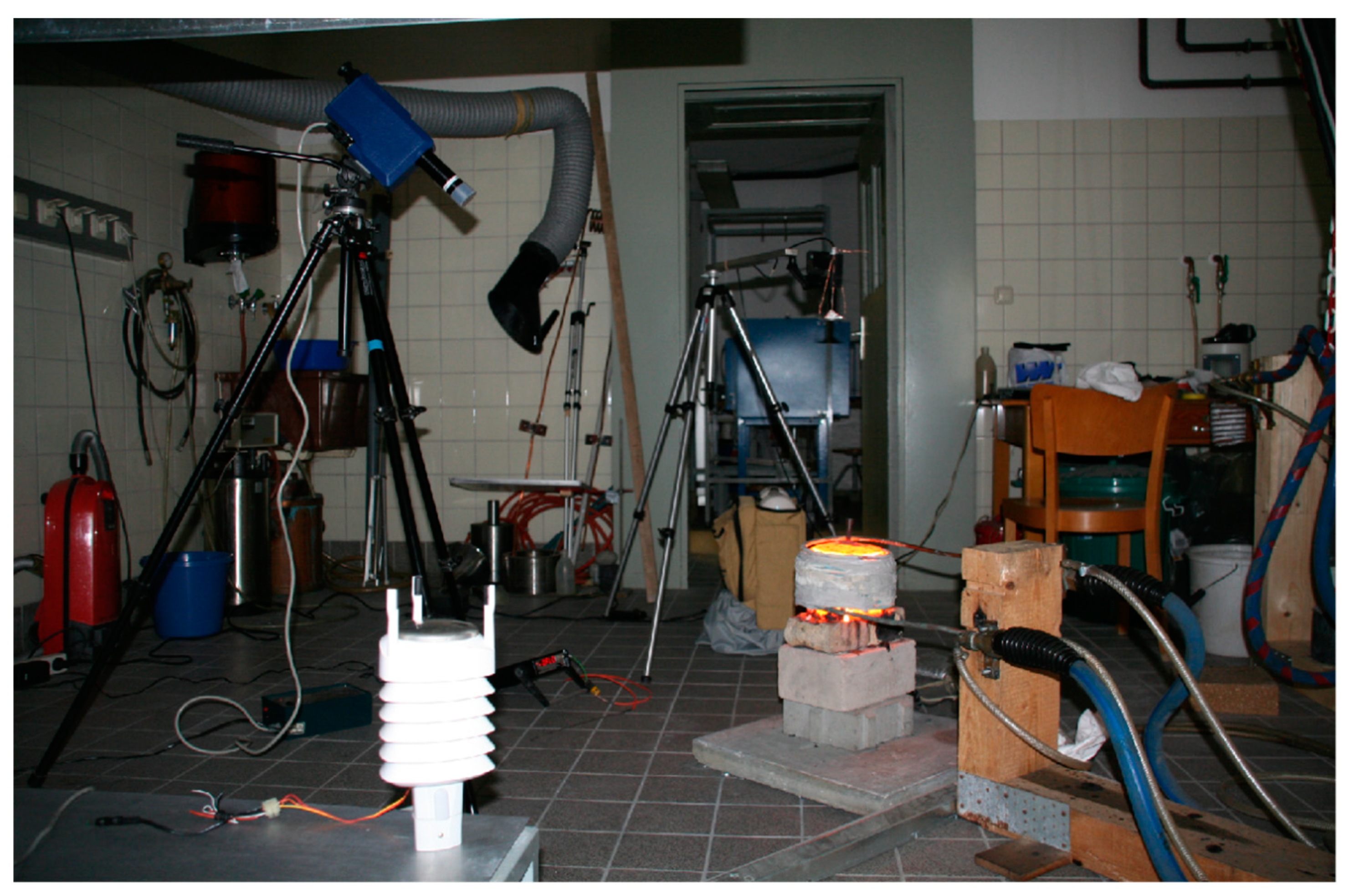
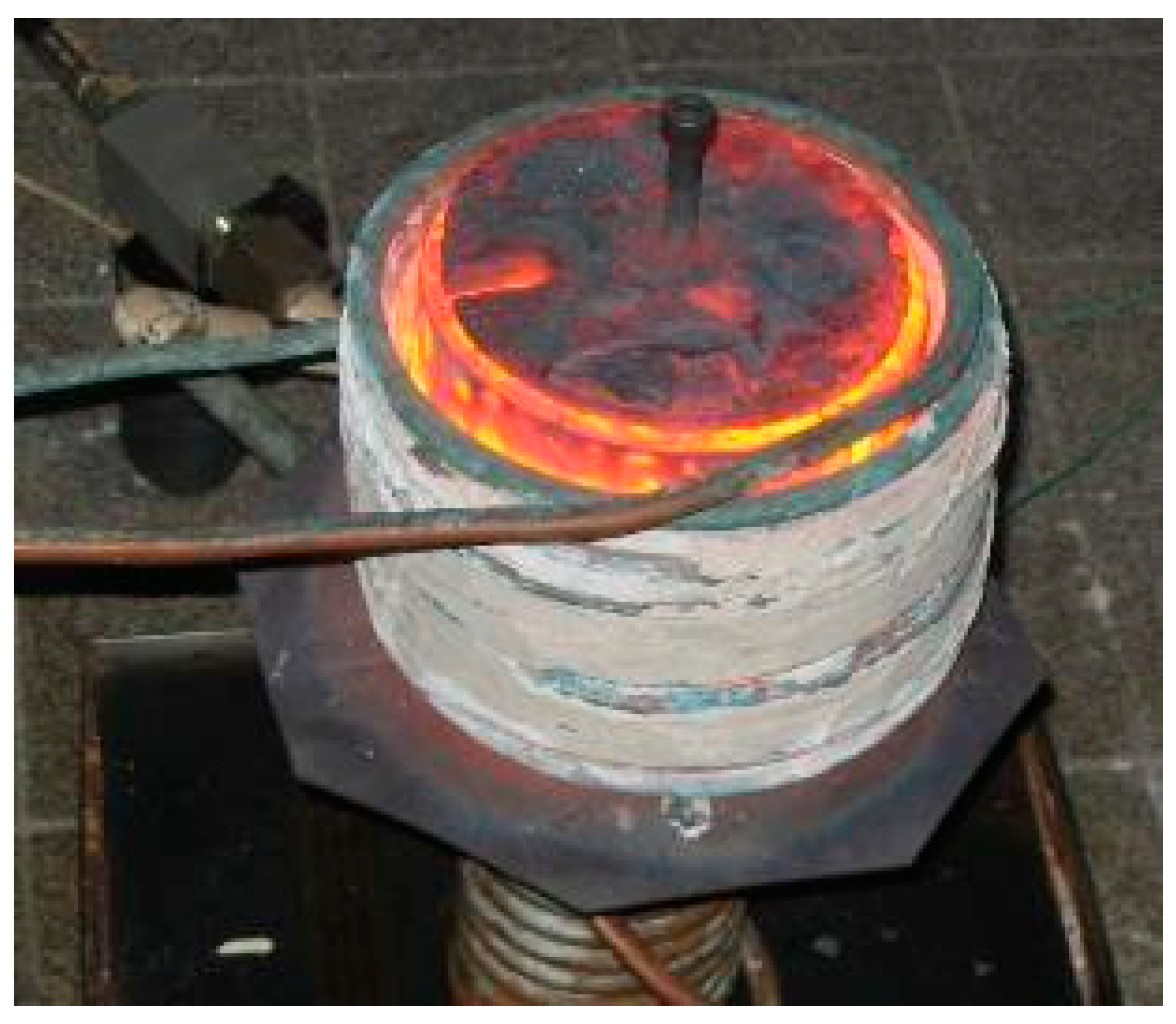
2.1. Experimental Data Acquisition

We collected spectra from non-thermally homogenous sources using the field-portable Spectroradiometer ASD FieldSpec Pro. The FieldSpec instrument is composed of three spectrometers which measure the spectral radiation energy in three different portions of the wavelength spectrum 350–2500 nm with a spectral resolution of 2–12 nm [38].

Volcanic bombs erupted from Mt. Etna during the 2002–03 eruption, trachybasaltic in composition [39], provided the starting material for the experiments. Post-experiment petrologic investigation confirmed that the experimental products, which we measured, and the starting material shared similar chemical compositions and mineral assemblages. In the Physical Volcanology Laboratory of the University of Würzburg (Figure 1), Germany, we melted about 0.3kg of granulate starting material in a 10 cm inner diameter steel crucible (Figure 2) inductively heated above magmatic temperature (>1500K) using a radio frequency generator [40]. Once the desired temperature was reached, the lid of the crucible was removed to expose the molten basalt to air, and its surface was remotely probed while cooling down over time until it reached a constant temperature, which was set by adjusting the power of the generator. The surface temperature of the basalt in the crucible was measured using an infrared pyrometer (Wintronics KT19.01 model, spectral range 2.0–2.7 µm, temperature range 520–2300 ±0.1 K, emissivity setting 0.1–1 in 0.001 increments, c-type sensor) and an S-type thermocouple (Pt/PtRh, temperature range 220–2000 K, tolerance 0.5%). In a darkroom environment, we collected spectra from the free surface of the melt using the field-portable FieldSpec.

2.2. Field of View and Data Saturation

The electromagnetic radiation emitted by the surface is collected by the instrument entry optics and projected into a holographic diffraction grating. The FieldSpec uses a bare fiber optic with a conical field of view (FOV) of 35°. However, the bare fibre FOV was further reduced using foreoptic tubes of 1° (Opt1) and 3° (Opt3), respectively. Foreoptics allow FieldSpec to focus on a smaller area than the entire melt surface. The diameter of the target area is a function of the distance between the FieldSpec and the lava surface. At a distance of 40 cm, as adopted during the experiments, the diameter of the target area measures 1.4cm and 4.0cm for foreoptics Opt1 and Opt3, respectively. Foreoptics also reduce detection errors caused by radiating energy in the FOV coming from the background outside of the melt. In this publication, we indicate with the term “pixel” the whole FOV of the used foreoptics.

In order to avoid instrumental saturation, we used two neutral density filters (F2 and F5;

Table 1. List of instrumental setups.

Setup	Foreoptic	Filter	Target Area Diameter	Max Unsaturated Temperature	Acquired Number of spectra
#1	Opt1	F2	1.4 cm	~1100 °C	40
#2	Opt1	F5	1.4 cm	~1300 °C	210
#3	Opt2	F2	4.0 cm	~1100 °C	50
#4	Opt2	F5	4.0 cm	~1300 °C	220

) to reduce the amount of radiation coming through the instrument in the SWIR region with an attenuation factor of 2 and 5, respectively. The higher attenuation filter (F5) guarantees unsaturated data and allows the inspection of higher ranges of lava temperature. The lower attenuation filter (F2) improves the radiometric measure, resolving smaller temperature variations. We acquired radiance spectra measurements of molten lava in four different setups, as summarised in Table 1.

2.3. Atmospheric Corrections

Atmospheric correction is the process of removing the effects of the atmosphere on radiance measured by remote sensors. The effect of atmospheric water vapour was investigated in our experiments by calculating the transmittance of the air column. We adopted the following water vapour transmittance expression T_w [41]:

T_w = EXP [−0.2385 × a_w × W × M/(1 + 20.07× a_w × W × M)^0.45],

(2)

where W is the precipitable water vapour in a vertical path; a_w is the water vapour absorption coefficient as a function of wavelength [42]; M is the air mass [43]. The water vapour amount W is not temperature- or pressure-corrected because this was accounted for in the form of Equation (2).

The coefficients a_w were calculated using precise laboratory air temperature, humidity and pressure values simultaneously recorded by a portable meteo-station. Figure 3 shows the difference between atmospherically corrected (black plot) and uncorrected (red plot) radiance spectra. As expected, the atmospheric column of 40 cm does not affect the spectra, except for the relatively slight differences of 1% that occur in the ranges 1350–1420 nm and 1770–2020 nm, which correspond to two main water vapour absorptions.

At a distance of 40cm from the crucible, in a ventilated confined environment, simulated atmospheric effects are negligible. However, the warm air column rising from the melt surface may cause absorption features in radiance spectra, due to water vapour heat-up. Such features cannot be fully predicted because our model does not allow changing gas temperatures in the simulation [44,45]. Therefore, our spectra will still show slight absorption due to water vapour.

2.4. Normalised Emissivity Method Applied to Molten Lava

Assuming a multispectral remote sensor recording SWIR spectral radiance from the surface in its field of view, the normalised emissivity method (NEM) is used to iteratively retrieve surface emissivity and temperature by assuming a maximum emissivity value. In the NEM algorithm, the maximum emissivity, ε_max, is assumed to be 0.99 [46]. The surface-emitted radiance R(λ), is related by the following equation to the reflected downwelling radiance R_d(λ) and the surface-leaving radiance R_surf (λ):

R(λ) = R_surf (λ)−(1−ε_max) × R_d(λ).

(3)

The NEM temperature T_N is defined as the maximum brightness temperature over all band wavelengths. The NEM temperature is used to calculate the apparent NEM emissivity (ε_Ν) by dividing the surface-leaving radiance by the blackbody radiance at temperature T_N:

ε_Ν(λ) = R(λ)/B(λ,T_N).

(4)

Replacing the maximum assumed emissivity with the apparent NEM emissivity the surface-emitted radiance R(λ) is:

R(λ) = R_surf (λ)–[1−ε_Ν(λ)] × R_d(λ).

(5)

The NEM algorithm iteratively removes the reflected downwelling radiance by refining its estimates of emissivity and temperature. In case of spaceborne sensors, the atmosphere interacts with the SWIR recorded spectral radiance, so its correction is critical for the temperature–emissivity algorithms. Atmospheric transmittances and radiances depend on the wavelength, so errors in the atmospheric correction are different in magnitude for each channel, which in turns implies that the derived emissivity spectra are inaccurate both in terms of amplitude and spectral variation. This is the case for the NEM method, where residual atmospheric effects could dictate the selection of T_N. Small variations in the input atmospheric profiles (10% in relative humidity) may lead to emissivity variations of 0.01–0.02 [47]. Following the approach described above, we attempt to retrieve the surface lava temperature T_s and the spectral emissivity ε(λ) from our DN spectra. However, our approach differs from that of Gillespie et al. [46] in two important ways.

First, SWIR data are used instead of TIR data. At magmatic temperatures, the peak wavelength of the radiation curve shifts towards the SWIR region and becomes evident in the measured spectral range 1300–2300 nm. Thus, we use the peak position to constrain T_s and reduce uncertainty in the emissivity estimation. Second, our corrected data clearly indicate that there is a negligible contribution of the atmospheric reflected downwelling radiance. This is due to the higher contribution of emitted radiance than the contribution of downwelling radiance that leaves the melt surface under laboratory conditions (e.g., dark environment and only 40cm of atmospheric path from sample surface to sensor). Starting from these assumptions, the emitted surface radiance equals the surface-leaving radiance:

R(λ) = ε(λ) × B(λ, T_s ) = R_surf (λ)

(6)

and the emissivity is:

ε(λ) = R(λ)/B(λ, T_s).

(7)

By using the NEM algorithm, one assumes a uniform temperature distribution within the lava surface, an assumption that does not apply to lava surfaces at sub-liquidus temperature.

2.5. The “Draping” Algorithm

Given the temperature heterogeneities observed in experimental melts, we have developed a new algorithm to take into account the radiance contribution due to surfaces radiating at different temperatures. In the following, we call the temperatures “sub-pixel temperatures”, which correspond to temperatures of different thermal components observed within a pixel.

We assume a thermal two-component model for the lava surface [16] in order to limit the number of unknowns. Following Dozier [48] and Rothery et al. [49], the radiance integrated over the area captured by the sensor FOV (A_fov) can be considered as a function of the fractional area of two thermally distinct surfaces. These are a cooler crust component at temperature T_c occupying the fraction f_c of FOV area A_fov and a high temperature component at temperature T_h, which occupies the remaining (1-f_c) portion of the A_fov area. The temperature T_h represents high-temperature molten lava. The radiance detected at one wavelength λ would be an average, weighted by the fractional area, of the two radiances related to the different temperatures:

R(λ, T_i) = ε(λ) × [f_h × R(λ, T_h) + (1 – f_h) × R(λ, T_c)],

(8)

where R is the Planck function for a blackbody radiating to temperature T at wavelength λ, T_i is the integrated temperature, and ε(λ) is the spectral emissivity. The Draping algorithm allows for the simultaneous calculation of T_h, T_c, f_h and ε(λ) throughout the following steps:

• Identify the largest radiance R_max over all available wavelengths.
• Create a lookup table of spectra derived from Equation (8) by varying T_h, T_c and f_h. Only spectra respecting the condition R(λ, T_i) ≥ R_max may be considered for comparison with measured radiances. This constraint guarantees that ε(λ) ≤ 1.
• Compute cross-correlation between radiance measurements and each spectrum of the lookup table and calculate the Spearman rank correlation coefficient.
• Identify the maximal Spearman rank correlation (T_i,,λ), which best matches the measured radiances and therefore identifies the triplet of values T_h, T_c and f_h fitting the thermal two-components model.

In the end, the spectral emissivity will be:

ε(λ) = R(λ)/(λ, T_i,).

(9)

3. Results

Results obtained by applying the Draping algorithm on spectral data measured from the experimental basaltic melt surfaces using the FieldSpec Pro are shown in Figure 4. The blue area represents the envelope of curves given from Equation (8) by varying T_h, T_c and f_h under the condition R(λ, T_i) ≥ R_max. T_h and T_c are forced to vary in the ranges 500–800 °C and 800–1200 °C, respectively. The variable f_h varies in the range 0.0–1.0 in steps of 0.01. The Spearman rank correlation coefficient is calculated to test the correlation between our experimental radiances and the theoretical radiances derived from Equation (8) using every triplet of T_h, T_c and f_h. The maximum value of the Spearman rank correlation coefficient individuates the best-fitting triplet.

Figure 5 shows the spectral emissivity derived from the cooling basalt sample at the sub-liquidus temperature of 1039 °C. The liquidus temperature specifies the temperature above which magma is entirely in a liquid state, i.e., the maximum temperature at which crystals can co-exist with the melt in thermodynamic equilibrium. Many igneous processes involve the flow of silicates at sub-liquidus temperatures, and therefore the simultaneous presence of a liquid and a crystalline phase.

Radiance spectra, collected at different temperatures, are quite stable and emissivity spectra overlap in the spectral range 1300–2500 nm. Emissivity profiles are similar in shape and magnitude, suggesting that spectral emissivity does not vary significantly in the investigated temperature range. The overall trend of the spectral profiles appears to be roughly constant with a mean of 0.96 and a standard deviation (σ_ε) of 0.011. This trend is interrupted by shallow dips in the ranges 1350–[0-9]{1,} nm and 1770–[0-9]{1,} nm, with values as low as 0.95 that correspond to the two main water vapour absorption bands. However, another shallow dip is visible in the ranges 2100–[0-9]{1,} nm centered at [0-9]{1,} nm, which cannot be attributed to standard atmospheric absorption bands. It is probably due to vibrational effects, which occur in basaltic melts at eruptive temperatures. This behaviour was observed in the higher temperature TIR emissivity spectra due to the changes in the vibrational behaviour of silicate melts [24].

The analysis of derived sub-pixel temperatures in Figure 6 shows that T_c ≈ T_h until a temperature of nearly 1120 °C is attained. At this point, we observe that T_c and T_h begin to diverge from each other. Whereas T_h appears to be constant at a temperature of about 1100 °C, T_c varies significantly during the cooling process.

4. Discussion

4.1. MethodValidation Using the Lava Simulator

For validation purposes, we applied the proposed methodology with the so-called lava simulator. This is a heat source made of a single heating wire alloy [50]. Electricity is converted into heat through Joule heating, with the heating power depending on the electrical current and the resistivity. As a proxy for the molten lava with temperature T_h, we used an alloy wire with a 0.5mm diameter made of Isachrom 60 (NiCr6015). For the crusted background with temperature T_c, a plywood panel painted with Senotherm spray (emissivity of 0.95) was used. A laboratory power supply unit provided a total maximal output of 400W. The experiment setup was located on a trolley, so it could be used at difference distances between the observing instruments and the lava simulator.

The changing distances were pivotal for the herein described experiment. Simultaneous observations with two thermal cameras at different distances made it possible to estimate the temperature, fractional area and emissivity of the hot wire [50]. The first of the thermal cameras (ImageIR 8300 – IR) made observations in two spectral regions (SWIR and MIR), the second one (VarioCam – VC) merely observed the TIR spectral region. The solution of Equation (8) is possible with only two thermal observations, given that:

• the temperature of the alloy is independent of the distance;
• the fraction of the alloy within the camera’s FOV (given as an angle in the product specification) is estimated based on the radius of the alloy and the distance to the camera;
• the temperature of the background is estimated from the pixels observing the plywood close to the alloy;
• two thermal observations in different spectral regions are available.

Therefore, two spectral emissivities remain unknown, but these can be estimated in an iterative solution. If we try different combinations of emissivities, we can find a solution with a small difference to the theoretical fraction of the alloy and a small variation of its temperature over all observed distances. These are the emissivities we are looking for. We ran our experiments with different combinations of SWIR, MIR and TIR datasets to estimate the wire emissivities in all three spectral regions. With emissivity steps of 0.05, we estimated the alloy’s emissivity to be 0.95 in the SWIR channel, in MIR, 0.85 and in TIR, 0.25 [50]. Such a strong variation in emissivity is not expected in the volcanic environment, however, because of the strong gradients, it is extremely interesting for validating the Draping method.

Considering the SWIR filter response, we computed a weighted average of the emissivities obtained from the Draping algorithm, resulting in a value of 0.93 for the IR’s SWIR band. Both emissivities are estimated independently, however, a difference of 0.02 is already a significant value. The difference of 0.02 is an acceptable deviation, considering that:

• the emissivity step in the iterative solution is 0.05;
• we only know the optical SWIR filter response and not the whole optics–sensor–electronics response;
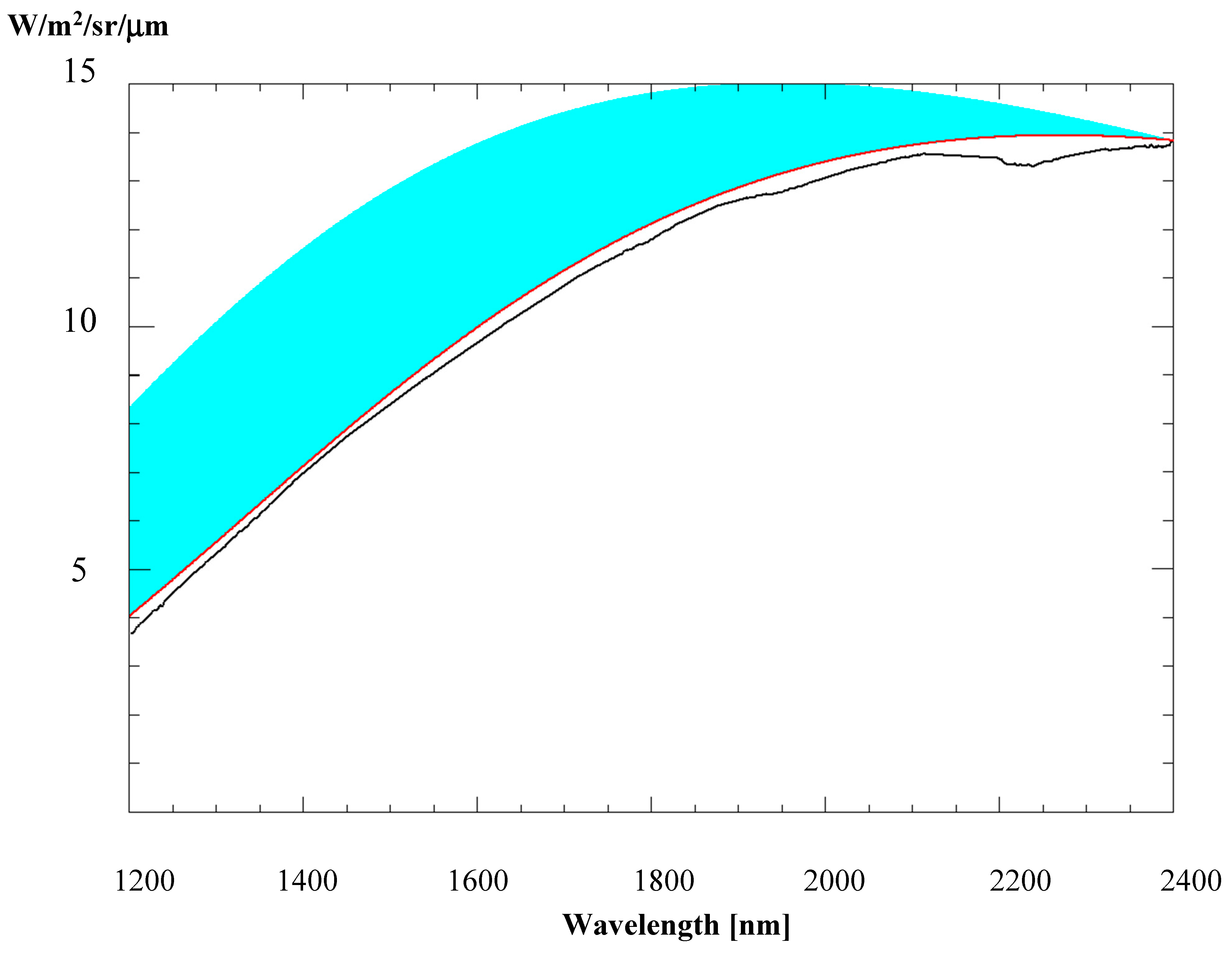
• the SWIR filter already covers a water absorption band (see the noise in Figure 6 at 2.5µm).

Figure 7 shows the hot alloy’s emissivity obtained by the Draping algorithm within the SWIR bandwidth, showing a decreasing trend towards the MIR band (>1.8 μm), as expected from the iterative solution.

The estimated emissivity made it possible to compute the temperature of the alloy (1292 °C) and temperature of the plywood panel (99 °C). For this we used a combination of MIR and TIR measurements and we obtained an error of 10 °C for the plywood panel and 39 °C for the alloy using the iterative method [50].

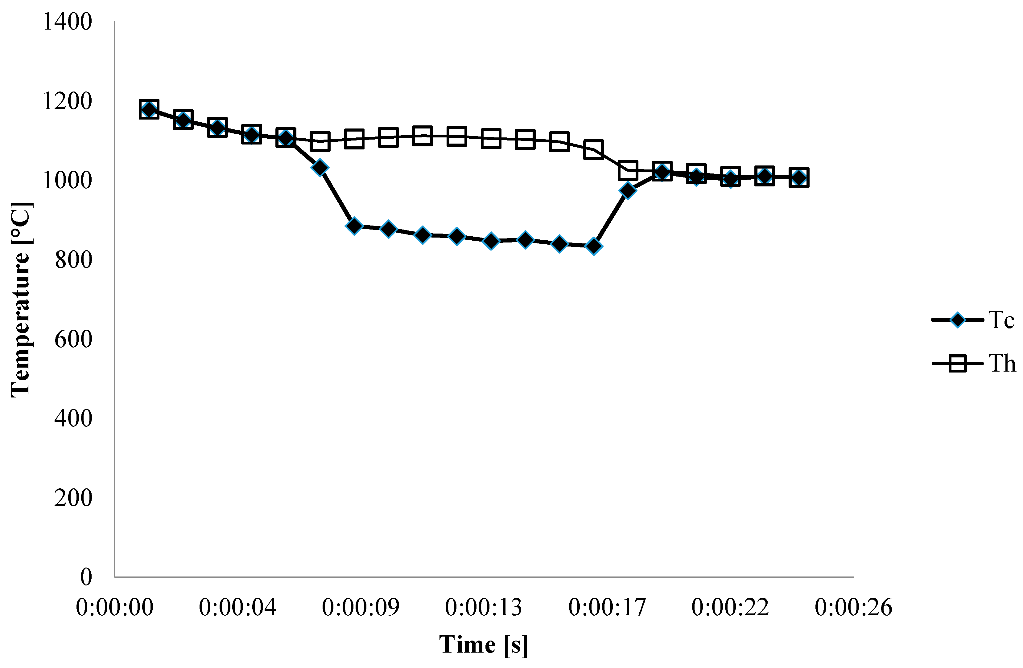
4.2. Sub-Pixel Temperatures

Figure 6 shows sub-pixel temperatures derived from radiance spectra using the draping algorithm. Temperatures were calculated during the cooling of the basaltic melt. The most relevant fact is the ability of the algorithm to discriminate different stages of the melt cooling:

• the first phase, in which the basalt is completely melted;
• the second phase, in which two thermal components are identified;
• the third phase, which corresponds to the complete solidification of the basalt.

This ability indicates the robustness of the proposed algorithm. However, it should be noted that in the two-component phase, the temperature of the cooler component (say the crust) seems to initially decrease and then increase again until it equals the temperature of the hot component. This behaviour is difficult to explain if we assume the hot and cold components always associate with the liquid and solid phases, respectively.

We must stress again that the algorithm is based on the assumption of a simple two-component thermal model for the melt. In fact, the proposed algorithm allows for the distinguishing of only two different thermal components. The model assumes, then identifies, these components as associated with the liquid and solid phases of the surface. However, preliminary temperature measurements with thermocouples indicate the presence of more than two thermal components during the second phase. Therefore, our two-component model could be too under-dimensioned to completely describe the molten surface temperature distribution [51,52]. Alternatively, the two components observed may represent different portions of the cooling crust with different cooling rates due to different radiating morphologies.

As the FieldSpec instrument has hundreds of bands in the SWIR region, the question may arise at this point: why should we not implement a solution describing more than two thermal components? The answer lies precisely in the fact that all our bands cover only the SWIR region. Lombardo et al. [53] demonstrated that the number of unknowns that can be calculated depends, not only on the number of available bands, but also on their position in the spectrum. Input data have uncertainties due to measurement limitations (instrument radiometric accuracy), which propagate the combination of variables in the system of equations (Equation (8)).

Lombardo et al. [53] performed a sensitivity analysis to determine the influence of the input data uncertainty on the output results (observational parameters).The trade-off among alternative band selections, the evaluation of atmospheric influence and radiometric accuracy were investigated. The accuracy of the retrieved thermal parameters changes significantly if different bands are involved in the computations. Solving a thermal three-components model by using three different SWIR bands yields large errors in sub-pixel temperature solutions [53]. This is because the SWIR region is limited with respect to the spectral range in which lava radiates at a molten temperature.

As shown in Figure 8, the accuracy in retrieved sub-pixel temperatures can be improved by adding a MIR band or a TIR band as input data in Equation (8). Unfortunately, the FieldSpec has no bands outside the SWIR portion of the spectrum.

4.3. Methodological Innovation Compared to Previous Methods for Temperature/Emissivity Separation

Numerous temperature and emissivity retrieval methods have been developed in recent decades. All these methods have different purposes and constraints in their applications. The target radiation measured by the sensor is a function of the emissivity of this target in the temperature during the measurement. From a mathematical point of view, the equations modelling this problem form an indeterminate system, where the number of measured variables exceeds the number of model equations (that is, the number of input radiance bands). In this form, the problem can never be solved because

N_unknowns = N_channels + N_parameters>N_channels

(10)

Each new equation brings a new unknown corresponding to the emissivity in that channel. The problem becomes much more complex if we consider further variables:

• parameters for atmospheric correction;
• more than a single temperature of the target at the sensor pixel scale (sub-pixel temperatures).

Therefore, the main point to be searched for is to obtain a method, even not optimal, but with a minimum of mathematical–physical restrictions and with the result of the lowest possible error. For a detailed discussion of these methods, we refer to Rolim et al. [36]. The main differences between these methods and our methodology essentially concern the temperature range of the target investigated, the spectral region examined, and the use of laboratory data. Herein, we want to focus on the peculiarities of our methodology.

The land surface emissivity (LSE) is the average emissivity of an element of the surface of the Earth calculated from measured radiance and land surface temperature (LST). Most of the methods in the literature refer to moderate temperature ranges [26,27,28,29,30,31,32,33,34,35,36,37]. As a result, these methods used the TIR spectral region to calculate LST. The magmatic temperature of lava varies between 800 °C and 1200 °C, so the peak of the emission shifts to shorter wavelengths (MIR and SWIR) as the temperature increases. There are not many studies on the emissivity of molten lavas.

Rogic et al. [25] investigated the role of emissivity in lava flow “distance-to-run”. Authors observed that TIR emissivity relating to the solidified (cooled) product does not reflect the range of temperatures involved in an active lava flow. They also demonstrated that a variation of 0.2 in emissivity may result in significant changes to the prediction of lava flow “distance-to-run” estimates.

Lee et al. [24] developed a micro furnace for use with a laboratory Fourier-transform infrared (FTIR) spectrometer and collected TIR emission spectra of actively melting and cooling silicate glasses. This is the experiment that comes closest to ours for setup and instrumentation. The TIR emissivity spectra of synthetic glasses and silicate melts were acquired. The authors experienced thermal heterogeneities in the sample and temperature fluctuations over time. The Draping algorithm allowed us, for the first time, to verify and quantify these thermal heterogeneities. Furthermore, by using a large diameter crucible (10 cm in inner diameter) it was possible to stabilise the temperature of the sample and minimise the effects of iron leaching. Once again, it must be highlighted that our innovative measurements refer to emissivity in the spectral region of SWIR.

The effectiveness of the Draping algorithm is based on two main factors:

• an accurate atmospheric correction of the data;
• the availability of high-spectral resolution(hyperspectral) data.

To analyse hyperspectral thermal data, it is necessary to correct the data for the atmospheric effects to retrieve the surface emissivity and temperature. Atmospheric parameters were calculated using precise laboratory air temperature, humidity and pressure values simultaneously recorded by a portable meteo-station. In our experiments, the contribution of emitted radiance from the lava surface is higher than the contribution of downwelling radiance. Our corrected data show that there is a negligible contribution of the atmospheric reflected downwelling radiance.

The Draping algorithm allows for simultaneously calculating the spectral emissivity and two sub-pixel temperatures using high-spectral resolution data. This is a three-step algorithm, which combines the original NEM algorithm [46] with a pre-estimate shape method [54] and a lookup table (LUT) to individuate the best sub-pixel temperatures to fit the thermal two-component model [55] of Equation (8). Given sufficient computational power, an exhaustive retrieval of the sub-pixel temperatures and the spectral emissivity can be performed.

FieldSpec allows the punctual acquisition of thousands of bands in the SWIR region. The next step will be the use of the Draping algorithm with satellite hyperspectral data. We plan to use the Draping algorithm with the PRecursore IperSpettrale della Missione Applicativa (PRISMA) sensor data. PRISMA is a medium-resolution hyperspectral imaging mission of the Italian Space Agency Agenzia Spaziale Italiana (ASI) launched in March 2019. PRISMA provides hyperspectral imagery (~250 bands) at a spatial resolution of 30 m on a swath of 30km. The spectral resolution is better than [0-9]{1,} nm in a spectral range of 400–[0-9]{1,} nm (VNIR and SWIR regions). The radiometric characteristics of this sensor make ASI-PRISMA a suitable instrument for observing high temperature events, such as volcanic eruptions and wildfires, and therefore a suitable instrument for testing the Draping algorithm on satellite data.

5. Conclusions

In this work, original experimental measurements of the spectral emissivity of Etnean basaltic melts were retrieved and presented. Due to the non-uniform temperature distribution of the basaltic melt surfaces, the new Draping algorithm for temperature/emissivity separation was implemented for the first time to simultaneously estimate the spectral emissivity and the sub-pixel temperatures in the SWIR region of the spectrum. The comparison between the cold and molten emissivities retrieved confirmed that the overall spectral emissivity does not vary significantly with magmatic temperature in the investigated SWIR spectral range. The sub-pixel temperatures appeared to vary widely during the cooling process of the silicate liquid. Future work will concern the investigation of the relationship between derived sub-pixel temperatures and thermal components of the lava during the cooling process.

In addition, an absorption feature in the range 2180–2290 nm was identified, which corresponded to an atmospheric window. This window is pivotal for the IR remote sensing of active volcanoes both from the ground and from space and therefore requires further investigations that can be done by exploring the acquisitions on active volcanoes of the new hyperspectral space mission ASI-PRISMA, in orbit since 2019.

References

1. Wan, Z.; Dozier, J. Land-surface temperature measurement from space: Physical principles and inverse modeling. IEEE Trans. Geosci. Remote Sens. 1989, 27, 268–278. [Google Scholar] [CrossRef] [Green Version]
2. Byrnes, J.M.; Ramsey, M.S.; King, P.L.; Lee, R.J. Thermal infrared reflectance and emission spectroscopy of quartzofeldspathic glasses. Geophys. Res. Lett. 2007, 34. [Google Scholar] [CrossRef] [Green Version]
3. Flynn, L.P.; Mouginis-Mark, P.J. Temperature of an active lava channel from spectral measurements, Kilauea Volcano, Hawaii. Bull Volcanol. 1994, 56, 297–301. [Google Scholar] [CrossRef]
4. Harris, A.J.L.; Blake, S.; Rothery, D.A.; Stevens, N.F. A chronology of the 1991 to 1993 Mount Etna eruption using advanced very high resolution radiometer data: Implications for real-time thermal volcano monitoring. J. Geophys. Res. 1997, 102, 7985–8003. [Google Scholar] [CrossRef]
5. Harris, A.J.L.; Flynn, L.P.; Keszthelyi, L.; Mouginis-Mark, P.J.; Rowland, S.K.; Resing, J.A. Calculation of lava effusion rates from Landsat TM data. Bull Volcanol. 1998, 60, 52–71. [Google Scholar] [CrossRef]
6. Wright, R.; Flynn, L.; Harris, A. Evolution of lava flow-fields at Mount Etna, 27-28 October 1999, observed by Landsat 7 ETM+. Bull. Volcanol. 2001, 63, 1–7. [Google Scholar] [CrossRef]
7. Andres, R.; Rose, W. Description of thermal anomalies on 2 active Guatemalan volcanos using Landsat Thematic Mapper imagery. Photogramm. Eng. Remote Sens. 1995, 61, 775–782. [Google Scholar]
8. Oppenheimer, C.; Francis, P.W.; Rothery, D.A.; Carlton, R.W.T.; Glaze, L.S. Infrared image analysis of volcanic thermal features: Láscar Volcano, Chile, 1984–1992. J. Geophys. Res. Solid Earth 1993, 98, 4269–4286. [Google Scholar] [CrossRef]
9. Wooster, M.J.; Kaneko, T.; Nakada, S.; Shimizu, H. Discrimination of lava dome activity styles using satellite-derived thermal structures. J. Volcanol. Geotherm. Res. 2000, 102, 97–118. [Google Scholar] [CrossRef]
10. Harris, A.J.; Rose, W.I.; Flynn, L.P. Temporal trends in lava dome extrusion at Santiaguito 1922–2000. Bull Volcanol. 2003, 65, 77–89. [Google Scholar] [CrossRef] [Green Version]
11. Glaze, L.S.; Francis, P.W.; Rothery, D.A. Measuring thermal budgets of active volcanoes by satellite remote sensing. Nature 1989, 338, 144–146. [Google Scholar] [CrossRef]
12. Oppenheimer, C.; Francis, P. Remote sensing of heat, lava and fumarole emissions from Erta ’Ale volcano, Ethiopia. Int. J. Remote Sens. 1997, 18, 1661–1692. [Google Scholar] [CrossRef]
13. Harris, A.J.L.; Flynn, L.P.; Rothery, D.A.; Oppenheimer, C.; Sherman, S.B. Mass flux measurements at active lava lakes: Implications for magma recycling. J. Geophys. Res. Solid Earth 1999, 104, 7117–7136. [Google Scholar] [CrossRef]
14. Oppenheimer, C.; Yirgu, G. Thermal imaging of an active lava lake: Erta ’Ale volcano, Ethiopia. Int. J. Remote Sens. 2002, 23, 4777–4782. [Google Scholar] [CrossRef]
15. Lombardo, V.; Harris, A.J.L.; Calvari, S.; Buongiorno, M.F. Spatial variations in lava flow field thermal structure and effusion rate derived from very high spatial resolution hyperspectral (MIVIS) data. J. Geophys. Res. Solid Earth 2009, 114. [Google Scholar] [CrossRef] [Green Version]
16. Crisp, J.; Baloga, S. A model for lava flows with two thermal components. J. Geophys. Res. Solid Earth 1990, 95, 1255–1270. [Google Scholar] [CrossRef]
17. Oppenheimer, C. Thermal distributions of hot volcanic surfaces constrained using three infrared bands of remote sensing data. Geophys. Res. Lett. 1993, 20, 431–434. [Google Scholar] [CrossRef]
18. Lombardo, V.; Buongiorno, M.F. Lava flow thermal analysis using three infrared bands of remote-sensing imagery: A study case from Mount Etna 2001 eruption. Remote Sens. Environ. 2006, 101, 141–149. [Google Scholar] [CrossRef]
19. Lombardo, V.; Buongiorno, M.; Amici, S. Characterization of volcanic thermal anomalies by means of sub-pixel temperature distribution analysis. Bull. Volcanol. 2006, 68, 641–651. [Google Scholar] [CrossRef]
20. Salisbury, J.W.; D’Aria, D.M. Emissivity of terrestrial materials in the 3–5 μm atmospheric window. Remote Sens. Environ. 1994, 47, 345–361. [Google Scholar] [CrossRef]
21. Buongiorno, M.F.; Realmuto, V.J.; Doumaz, F. Recovery of spectral emissivity from Thermal Infrared Multispectral Scanner imagery acquired over a mountainous terrain: A case study from Mount Etna Sicily. Remote Sens. Environ. 2002, 79, 123–133. [Google Scholar] [CrossRef]
22. Pieri, D.C.; Glaze, L.S.; Abrams, M.J. Thermal radiance observations of an active lava flow during the June 1984 eruption of Mount Etna. Geology 1990, 18, 1018–1022. [Google Scholar] [CrossRef]
23. Spinetti, C.; Mazzarini, F.; Casacchia, R.; Colini, L.; Neri, M.; Behncke, B.; Salvatori, R.; Buongiorno, M.F.; Pareschi, M.T. Spectral properties of volcanic materials from hyperspectral field and satellite data compared with LiDAR data at Mt. Etna. Int. J. Appl. Earth Obs. Geoinf. 2009, 11, 142–155. [Google Scholar] [CrossRef]
24. Lee, R.J.; Ramsey, M.S.; King, P.L. Development of a new laboratory technique for high-temperature thermal emission spectroscopy of silicate melts. J. Geophys. Res. Solid Earth 2013, 118, 1968–1983. [Google Scholar] [CrossRef] [Green Version]
25. Rogic, N.; Cappello, A.; Ferrucci, F. Role of Emissivity in Lava Flow ‘Distance-to-Run’ Estimates from Satellite-Based Volcano Monitoring. Remote Sens. 2019, 11, 662. [Google Scholar] [CrossRef] [Green Version]
26. Paul, M.; Aires, F.; Prigent, C.; Trigo, I.F.; Bernardo, F. An innovative physical scheme to retrieve simultaneously surface temperature and emissivities using high spectral infrared observations from IASI. J. Geophys. Res. Atmos. 2012, 117. [Google Scholar] [CrossRef] [Green Version]
27. Li, J.; Li, J.; Weisz, E.; Zhou, D.K. Physical retrieval of surface emissivity spectrum from hyperspectral infrared radiances. Geophys. Res. Lett. 2007, 34. [Google Scholar] [CrossRef] [Green Version]
28. Pivovarník, M.; Khalsa, S.J.S.; Jiménez-Muñoz, J.C.; Zemek, F. Improved Temperature and Emissivity Separation Algorithm for Multispectral and Hyperspectral Sensors. IEEE Trans. Geosci. Remote Sens. 2017, 55, 1944–1953. [Google Scholar] [CrossRef]
29. Cheng, J.; Liu, Q.; Li, X.; Xiao, Q.; Liu, Q.; Du, Y. Correlation-based temperature and emissivity separation algorithm. Sci. China Ser. D-Earth Sci. 2008, 51, 357–369. [Google Scholar] [CrossRef]
30. Borel, C. Error analysis for a temperature and emissivity retrieval algorithm for hyperspectral imaging data. Int. J. Remote Sens. 2008, 29, 5029–5045. [Google Scholar] [CrossRef]
31. Cheng, J.; Liang, S.; Wang, J.; Li, X. A Stepwise Refining Algorithm of Temperature and Emissivity Separation for Hyperspectral Thermal Infrared Data. IEEE Trans. Geosci. Remote Sens. 2010, 48, 1588–1597. [Google Scholar] [CrossRef]
32. Wang, N.; Wu, H.; Nerry, F.; Li, C.; Li, Z.-L. Temperature and Emissivity Retrievals from Hyperspectral Thermal Infrared Data Using Linear Spectral Emissivity Constraint. IEEE Trans. Geosci. Remote Sens. 2011, 49, 1291–1303. [Google Scholar] [CrossRef]
33. Zhang, Y.-Z.; Wu, H.; Jiang, X.-G.; Jiang, Y.-Z.; Liu, Z.-X.; Nerry, F. Land Surface Temperature and Emissivity Retrieval from Field-Measured Hyperspectral Thermal Infrared Data Using Wavelet Transform. Remote Sens. 2017, 9, 454. [Google Scholar] [CrossRef] [Green Version]
34. Dash, P.; Göttsche, F.-M.; Olesen, F.-S.; Fischer, H. Land surface temperature and emissivity estimation from passive sensor data: Theory and practice-current trends. Int. J. Remote Sens. 2002, 23, 2563–2594. [Google Scholar] [CrossRef]
35. Hulley, G.C.; Hook, S.J.; Abbott, E.; Malakar, N.; Islam, T.; Abrams, M. The ASTER Global Emissivity Dataset (ASTER GED): Mapping Earth’s emissivity at 100 meter spatial scale. Geophys. Res. Lett. 2015, 42, 7966–7976. [Google Scholar] [CrossRef]
36. Rolim, S.B.A.; Grondona, A.; Hackmann, C.L.; Rocha, C. A Review of Temperature and Emissivity Retrieval Methods: Applications and Restrictions. Am. J. Environ. Eng. 2016, 6, 119–128. [Google Scholar]
37. Sabol, D.E., Jr.; Gillespie, A.R.; Abbott, E.; Yamada, G. Field validation of the ASTER Temperature–Emissivity Separation algorithm. Remote Sens. Environ. 2009, 113, 2328–2344. [Google Scholar] [CrossRef]
38. Analytical Spectral Devices Inc. FieldSpec Pro User’s Guide; Analytical Spectral Devices Inc.: Boulder, CO, USA, 2002. [Google Scholar]
39. Andronico, D.; Branca, S.; Calvari, S.; Burton, M.; Caltabiano, T.; Corsaro, R.A.; Del Carlo, P.; Garfì, G.; Lodato, L.; Miraglia, L.; et al. A multi-disciplinary study of the 2002–03 Etna eruption: Insights into a complex plumbing system. Bull Volcanol. 2005, 67, 314–330. [Google Scholar] [CrossRef]
40. Büttner, R.; Dellino, P.; Raue, H.; Sonder, I.; Zimanowski, B. Stress-induced brittle fragmentation of magmatic melts: Theory and experiments. J. Geophys. Res. Solid Earth 2006, 111. [Google Scholar] [CrossRef] [Green Version]
41. Leckner, B. The spectral distribution of solar radiation at the earth’s surface—Elements of a model. Sol. Energy 1978, 20, 143–150. [Google Scholar] [CrossRef]
42. Bird, R.E.; Riordan, C. Simple Solar Spectral Model for Direct and Diffuse Irradiance on Horizontal and Tilted Planes at the Earth’s Surface for Cloudless Atmospheres. J. Clim. Appl. Meteor. 1986, 25, 87–97. [Google Scholar] [CrossRef] [Green Version]
43. Kasten, F. A new table and approximation formula for the relative optial air mass. Arch. Met. Geoph. Biokl. B 1965, 14, 206–223. [Google Scholar] [CrossRef]
44. Berk, A.; Bernstein, L.S.; Robertson, D.C. Modtran: A Moderate Resolution Model for Lowtran 7; Air Force Geophysics Laboratory: Hanscom AFB, MA, USA, 1994; p. 42. [Google Scholar]
45. Kneizys, F.X.; Abreu, L.W.; Anderson, G.P.; Chetwynd, J.H.; Berk, A.; Bernstein, L.S.; Robertson, D.C.; Albert, P.; Rothman, L.S.; Selby, J.E.A.; et al. The Modtran 2/3 Report and Lowtran 7 Model; Ontar Corporation USA: Hanscom AFB, MA, USA, 1996; p. 261. [Google Scholar]
46. Gillespie, A.R.; Matsunaga, T.; Rokugawa, S.; Hook, S.J. Temperature and emissivity separation from Advanced Spaceborne Thermal Emission and Reflection Radiometer (ASTER) images. IEEE Trans. Geosci. Remote Sens. 1998, 36, 1113–1126. [Google Scholar] [CrossRef]
47. Coll, C.; Caselles, V.; Schmugge, T.J. Imation of land surface emissivity differences in the split-window channels of AVHRR. Remote Sens. Environ. 1994, 48, 127–134. [Google Scholar] [CrossRef]
48. Dozier, J. A method for satellite identification of surface temperature fields of subpixel resolution. Remote Sens. Environ. 1981, 11, 221–229. [Google Scholar] [CrossRef]
49. Rothery, D.A.; Francis, P.W.; Wood, C.A. Volcano monitoring using short wavelength infrared data from satellites. J. Geophys. Res. 1988, 93, 7993–8008. [Google Scholar] [CrossRef]
50. Pick, L.; Lombardo, V.; Zakšek, K. Assessment of Dual-Band method with Indoor Analog Experiment. Ann. Geophys. 2019, 62, 219. [Google Scholar] [CrossRef]
51. Rose, S.R.; Watson, I.M.; Ramsey, M.S.; Hughes, C.G. Thermal deconvolution: Accurate retrieval of multispectral infrared emissivity from thermally-mixed volcanic surfaces. Remote Sens. Environ. 2014, 140, 690–703. [Google Scholar] [CrossRef]
52. Wright, R.; Flynn, L.P. On the retrieval of lava-flow surface temperatures from infrared satellite data. Geology 2003, 31, 893–896. [Google Scholar] [CrossRef]
53. Lombardo, V.; Musacchio, M.; Buongiorno, M.F. Error analysis of subpixel lava temperature measurements using infrared remotely sensed data. Geophys. J. Int. 2012, 191, 112–125. [Google Scholar] [CrossRef] [Green Version]
54. Lan, X.; Zhao, E.; Li, Z.-L.; Labed, J.; Nerry, F. An Improved Linear Spectral Emissivity Constraint Method for Temperature and Emissivity Separation Using Hyperspectral Thermal Infrared Data. Sensors 2019, 19, 5552. [Google Scholar] [CrossRef] [Green Version]
55. Lombardo, V.; Silvestri, M.; Spinetti, C. Near-real time routine for volcano monitoring using IR satellite data. Ann. Geophys. 2011, 54, 522–534. [Google Scholar] [CrossRef]
Figure 1. Experimental setup: basaltic rocks are melted in a steel crucible inductively heated using a radio frequency generator. In the background: the high spectral resolution portable spectrometer FieldSpec Pro for acquiring radiance spectra. To the left: thermocouple, pyrometer, and a thermal camera for providing punctual and spatially independent temperature measurements of the molten material. In the foreground: a portable meteo-station for continuously recording atmospheric ambient parameters to remove the effects of the atmosphere on acquired radiance spectra.
Remotesensing 12 02046 g001
Figure 2. The steel crucible (10 cm inner diameter) with its lid during the melting phase of an experiment.
Remotesensing 12 02046 g002
Figure 3. Comparison between measured spectral radiances (black) and atmospherically corrected radiances (red) exposes spectral regions with significant influence on atmospheric features.
Remotesensing 12 02046 g003
Figure 4. Solutions from the application of the Draping algorithm on spectral data (SD) measured from a basaltic melt surface. The blue area represents the envelope of curves given from Equation (8) by varying Th, Tc and fh under the condition R(λ, Ti,) ≥ Rmax. The maximum value of the Spearman rank correlation coefficient individuates the best fit curve (BF) and therefore the triplet of values Th, Tc and fh that best fit the thermal two-component model (red curve).
Remotesensing 12 02046 g004
Figure 5. High radiometric accuracy spectral emissivity of a basaltic melt at 1042 °C, derived using the Draping algorithm. A broad absorption feature is visible in the range 2180–2290 nm centred at about 2220 nm. It is probably an overtone vibrational band of the silicate mineralogy due to the fact that the basalt is molten.
Remotesensing 12 02046 g005
Figure 6. Sub-pixel temperatures derived from radiance spectra using the Draping algorithm. Assuming a thermal two-component model for our basaltic melts, we individuate three phases in the cooling process based on the number of derived components. Measurements were collected starting from completely molten lava at 1200 °C.
Remotesensing 12 02046 g006
Figure 7. Spectral emissivity of the hot wire of the lava simulator derived with the Draping algorithm. Grey area: SWIR filter of IR camera. Dashed lines: emissivity (0.93) at filter’s central wavelength (2.36 μm).
Remotesensing 12 02046 g007
Figure 8. Radiance spectrum derived from Equation (8) using values of 1200 K, 500 K and 0.003 for Tc, Th and fh, respectively. Red curves show uncertainties for an absolute radiometric accuracy of 0.03. Dots show the location of 1.6 and 2.2 μm SWIR bands within this spectral profile. The SWIR region covers only a small portion of the radiance spectrum (corresponding to the steep slope S1–S2), therefore it is difficult to solve the unconstrained system of equations (Equation (8)) by adding another SWIR band.
Remotesensing 12 02046 g008