Article

Near Real-Time Automated Early Mapping of the Perimeter of Large Forest Fires from the Aggregation of VIIRS and MODIS Active Fires in Mexico

by
Carlos Ivan Briones-Herrera
1,
Daniel José Vega-Nieva
1,*,
Norma Angélica Monjarás-Vega
1,
Jaime Briseño-Reyes
1,
Pablito Marcelo López-Serrano
1,
José Javier Corral-Rivas
1,
Ernesto Alvarado-Celestino
2,
Stéfano Arellano-Pérez
3,
Juan Gabriel Álvarez-González
3,
Ana Daría Ruiz-González
3,
William Mathew Jolly
4 and
Sean A. Parks
5
1
Facultad de Ciencias Forestales, Universidad Juárez del Estado de Durango, Río Papaloapan y Blvd, Durango S/N Col. Valle del Sur, 34120 Durango, Mexico
2
School of Environmental and Forest Sciences, University of Washington, Mailbox 352100, University of Washington, Seattle, WA 98195, USA
3
Departamento de Ingeniería Agroforestal, Universidad de Santiago de Compostela, Escuela Politécnica Superior de Ingeniería, Campus Universitario s/n, 27002 Lugo, Spain
4
USDA Forest Service, Missoula Fire Sciences Laboratory, Missoula, MT 59808, USA
5
USDA Forest Service, Aldo Leopold Wilderness Research Institute, Rocky Mountain Research Station, Missoula, MT 59801, USA
*
Author to whom correspondence should be addressed.
Remote Sens. 2020, 12(12), 2061; https://0-doi-org.brum.beds.ac.uk/10.3390/rs12122061
Submission received: 1 June 2020 / Revised: 14 June 2020 / Accepted: 23 June 2020 / Published: 26 June 2020

Abstract

:
In contrast with current operational products of burned area, which are generally available one month after the fire, active fires are readily available, with potential application for early evaluation of approximate fire perimeters to support fire management decision making in near real time. While previous coarse-scale studies have focused on relating the number of active fires to a burned area, some local-scale studies have proposed the spatial aggregation of active fires to directly obtain early estimate perimeters from active fires. Nevertheless, further analysis of this latter technique, including the definition of aggregation distance and large-scale testing, is still required. There is a need for studies that evaluate the potential of active fire aggregation for rapid initial fire perimeter delineation, particularly taking advantage of the improved spatial resolution of the Visible Infrared Imaging Radiometer (VIIRS) 375 m, over large areas and long periods of study. The current study tested the use of convex hull algorithms for deriving coarse-scale perimeters from Moderate Resolution Imaging Spectroradiometer (MODIS) and Visible Infrared Imaging Radiometer Suite (VIIRS) active fire detections, compared against the mapped perimeter of the MODIS collection 6 (MCD64A1) burned area. We analyzed the effect of aggregation distance (750, 1000, 1125 and 1500 m) on the relationships of active fire perimeters with MCD64A1, for both individual fire perimeter prediction and total burned area estimation, for the period 2012–2108 in Mexico. The aggregation of active fire detections from MODIS and VIIRS demonstrated a potential to offer coarse-scale early estimates of the perimeters of large fires, which can be available to support fire monitoring and management in near real time. Total burned area predicted from aggregated active fires followed the same temporal behavior as the standard MCD64A1 burned area, with potential to also account for the role of smaller fires detected by the thermal anomalies. The proposed methodology, based on easily available algorithms of point aggregation, is susceptible to be utilized both for near real-time and historical fire perimeter evaluation elsewhere. Future studies might test active fires aggregation between regions or biomes with contrasting fuel characteristics and human activity patterns against medium resolution (e.g., Landsat and Sentinel) fire perimeters. Furthermore, coarse-scale active fire perimeters might be utilized to locate areas where such higher-resolution imagery can be downloaded to improve the evaluation of fire extent and impact.

Graphical Abstract

1. Introduction

In spite of the large importance of burned area monitoring for carbon cycle and emissions accounting [1], there is still much uncertainty in the area affected by biomass burning [2,3,4,5]. Two types of satellite data products have been used for mapping fire occurrence: active fire and burned area products [4]. Burned area products are generally based on reflectance changes [6] or on the combination of reflectance with active fires [5,7,8,9], while active fires are based on thermal anomalies detection [10,11]. Global burned area products [8] are utilized to feed the Global Fire Emissions Database (GFED), combined with empirical relationships to estimate the contribution of small fires (not detected by coarse-resolution burned area products) from Moderate Resolution Imaging Spectroradiometer (MODIS) active fires [1,5,12].
Current operational products of global burned area [8] are generally available one month after the fire, limiting their applicability for fire near real-time perimeter monitoring [13,14,15] which can be useful for fire managers to make early evaluations of approximate fire extent and location. Unlike current products of burned area data, observations of active fires made with spaceborne sensors are available at least with a daily latency [11,16,17]. Therefore, available near-real-time active fires are often used as an approximation to estimate burned area [1,2,3,12,16,18,19,20,21,22].
Several studies have attempted to relate the number of active fire detections with observed monthly burned area from medium- to coarse-resolution sensors. Such analyses have ranged from global studies, generally utilizing gridded active fire counts at pixels of 15 km to 0.5 ° [12,16,18,23,24], to local scales, the latter generally calibrated against satellite burned area and/or field-measured fire perimeters [3,25,26,27]. This approach has been generally acknowledged to be challenging [3,16] because of variability in cloud cover, fuel, topography, weather and associated fire behavior, together with issues related to spatial and temporal resolution of the imagery [3,4,25,26,27,28,29]. In addition, some authors have also found that the relationships between the number of active fire detections and burned area can be largely influenced by the size of the monthly cumulative active fire clusters [2,16].
Instead of using the number of active fire pixels, other studies, mainly at local scales, have proposed to directly utilize the aggregation of active fire detections to delineate approximate fire perimeters. Some studies have even tested such interpolations of conglomerates of active fires to visualize the approximate advance of the perimeter of large fires [13,14,30,31,32,33,34,35] and to calibrate fire propagation models [36,37,38,39,40,41,42,43,44]. Several techniques are being investigated for this aggregation approach, including the direct aggregation or buffering of active fires (e.g., [30,31]), the inverse distance weighted or the weighted mean and distance methods (e.g., [13]), kriging analysis (e.g., [14]), or the use of convex hull algorithms applied to active fire clusters (e.g., [15,43]).
Currently, the majority of the literature relating active fire detections to burned areas has been conducted with coarse-resolution sensors, mainly with 1 km resolution, such as Advanced very-high-resolution radiometer (AVHRR) [19,25,26,27] or MODIS [3,14,30,32,33]. While those studies showed that first-order burned area estimates can be obtained from 1 km satellite active fire data, it is widely recognized that higher spatial and temporal resolutions are needed to explore the possibility of direct fire perimeter mapping from active fires [31]. The more recently available Visible Infrared Imaging Radiometer (VIIRS) aboard the Suomi National Polar-orbiting Partnership (S-NPP) satellite, launched in 2011, offers greater potential for small fire detection, having a higher temporal and spatial resolution (375 m) [11,45,46]. Such enhanced characteristics of the VIIRS 375 m active fire product reopened the possibility of direct rapid mapping of burned areas from active fire detection products [15,31].
In spite of this potential, studies testing the use VIIRS active fires for fire perimeter monitoring are still scarce [15,31]. The study of Oliva and Schroeder [31] demonstrated the potential of VIIRS active fires aggregation for mapping fire perimeters, in 10 selected local scenes at several countries with contrasting vegetation types, in the year 2013. Although this study showed great promise for the operational use of VIIRS active fires interpolation for burned area prediction, further testing is required in different regions and seasons [31], at larger areas of study, both at individual fire perimeter and regional or country total burned area levels. The approach tested in this study was the direct aggregation of spatially contiguous pixels [30,31,47]. Other active fire cluster aggregation techniques, such as the alpha shape algorithm, a generalization of the convex hull envelope developed by Chiaraviglio et al. [32], have been recently tested, with promising results for individual fire perimeter rapid delineation. The assessment of this algorithm for total burned area prediction based on MODIS and VIIRS active fires [15], and the algorithm parameter optimization, are still ongoing tasks (Artés, personal communication, 2019), for which a long-term evaluation against burned area records is still required. In this sense, the optimization of active fire clustering algorithms requires a minimum of domain knowledge to determine the input parameters and interpolate large databases with irregular shapes with good precision [48]. To our best knowledge, we are not aware of previous studies that have analyzed how the aggregation distance of MODIS and VIIRS active fires affects its potential to estimate burned area both at the individual fire perimeter and total sum of burned area levels, over large areas and long periods of study.
The current study is aimed at evaluating the potential of MODIS and VIIRS active fires aggregated perimeters to estimate monthly burned area in Mexico for the period 2012–2018. The study analyzed the role of the aggregation distance of MODIS and VIIRS active fires in the prediction of burned area, as measured by the current standard MCD64A1 burned area product [8], both at individual fire perimeter level and total sum of burned area, in Mexican forest lands.

2. Materials and Methods

2.1. Study Area, Burned Area and Active Fires Data

The study area included the natural forest vegetation of Mexican territory. Areas corresponding to agriculture, water bodies and human settlements were excluded from the analysis, according to the most recent Land-Use Map VI (1: 250,000) from the National Institute of Geography and Statistics (INEGI) [49] (Figure 1). Note that here the term “forest” is used in a broad sense. In fact, Northern Mexico and Baja California natural vegetation areas comprise a mix of shrubby and wooded vegetation, the former being by far the dominant cover in both regions [50].
The period of study was from January 2012 to June 2018. While fire season in Mexico is mainly concentrated in the months of March to June [51,52], burned area and active fires from all months in the period of study were considered. Monthly burned area perimeters from the study period were downloaded from the FTP server of the University of Maryland. Burned area perimeters corresponded to the collection C6 burned area (MCD64A1) at a spatial resolution of 500 m [8]. Details about the burned area product are included in the user guide (http://modis-fire.umd.edu/files/MODIS_C6_BA_User_Guide_1.2.pdf). The active fires from the Moderate Resolution Imaging Radiometer Spectrum (MODIS, C6) [10] and the active fires data from the Visible Infrared Imaging Radiometer Suite (VIIRS, V1, 375 m) [11], for the study period, were downloaded from the Fire Information for Resource Management System (FIRMS, https://firms.modaps.eosdis.nasa.gov/download/create.php).

2.2. Predicting Burned Area from Aggregation of Active Fires

Interpolated perimeters from the monthly accumulated active fires MODIS and VIIRS were generated using a convex hull aggregation with the “aggregate points” tool in ArcGIS (ESRI; 2011, Redlands, CA, USA) [53]. The convex hull algorithm delineates an area containing clusters of points (3 points minimum) at a specified aggregation distance. Four aggregation distances, 750, 1000, 1125 and 1500 m, were tested for perimeter delineation. Tested distances were chosen based on the spatial resolution of the active fires from VIIRS (375 m) and MODIS (1000 m). The minimum aggregation distance was defined as two VIIRS pixels to account for possible errors in pixel geolocation. Interpolated perimeters were compared with the coinciding burned areas perimeters of the C6 MCD64A1 product that occurred in the same month, year and location. When two or more active fire interpolated perimeters coincided spatial and temporally with a single burned area perimeter, the sum of their area was considered for analysis. The delimitation of the aggregated perimeters from active fire data was automated using the arcpy package included in the PyCharm 2019.3.1 software (JetBrains, 2017) [54]. The code is available upon request to the corresponding author, and can be utilized both for historical data and near real time active fire perimeter delimitation.
The following models were tested to predict the MCD64A1 burned area from the aggregated perimeter of the active fires at 750, 1000, 1125 and 1500 m using the following Equation (1):
BA = a·x
where: BA: MODIS C6 MCD64A1 burned area (ha); a: model parameter; x: aggregated perimeter of active fires (ha), respectively.
The models were tested at two levels: (1) individual fire perimeter burned area; (2) total monthly sum of burned area. The database for the period of study comprised a total of 5218 burned area individual fire perimeters, with an average surface of 2305 ha and a standardized deviation of 3200 ha. For the monthly sum of burned area evaluation, a total of 79 monthly observations in the study period were utilized. Total monthly sum of burned area averaged 73,622 ha, with a standardized deviation of 122,749 ha. The models were fitted with linear regression using the command “lm” within the R statistical platform (R Core Team, 2017 Vienna, Austria) [55]. Candidate models were evaluated using the coefficient of determination (R2), root mean square error (RMSE) and model bias (average of observed minus predicted values) [56]. In addition, the presence of heteroscedasticity was analyzed by use of the White test [57]. If observed, each observation would be weighted by the inverse of its estimated variance, assuming that this variance can be modelled as a power function of the aggregated perimeter of active fires (x) and optimizing the exponential term to provide the most homogeneous Studentized residual plot. Anyway, this problem may affect the standard error estimate of parameter a, but the least-square estimate of this parameter would remain unbiased and consistent even in the presence of heteroscedasticity [58], therefore, while it might not be completely corrected, it would be irrelevant in this study.

2.3. Case Study with Sentinel Fire Perimeters

An illustrative evaluation of the aggregated perimeters and MODIS burned area against Sentinel perimeters was performed for 3 selected example fires from 2019 where field data to calibrate burned area perimeter was available. Study areas were dominated with pine and oak forests with tree covers ranging from <5% to 55%, combined with desert shrubland and natural pasture vegetation. Sentinel 2C pre- and post-fire surface reflectance images with the lowest cloud cover were downloaded from Google Earth Engine utilizing a modification of the automated code from Parks et al. [59] for Sentinel. The code requires the specification of initial perimeter location, which was defined from the aggregated active fire perimeters. For the phenological correction to account for phenology-caused changes in the burnt area indices [59], unburnt areas were defined as a buffer from 3 km to 5 km away from the aggregated active fire perimeter, to account for potential geolocation and active fire cloud obscuration errors. The phenologically corrected difference normalized burn ratio (dNBRcorr) [59] was calculated utilizing Sentinel 2C bands 12 and 8a (https://developers.google.com/earth-engine/datasets/catalog/COPERNICUS_S2_SR#bands, accessed June 24, 2020). Based on 100 field plots in the selected fires, the threshold of burnt area was defined as a dNBRcorr >100 for the areas of study. Agreement, commission and omission errors were evaluated for both the aggregated active fire and MODIS burned area for the 3 selected example Sentinel perimeters.

3. Results

The goodness of fit of the models to predict burned area from aggregation distances of active fires varied between the considered aggregation distance (Table 1). The best goodness of fit for the linear function for individual fire prediction were obtained for the distance of 1125 m, which also showed the a coefficient value closest to 1 (Table 1) and a bias value closest to 0, (a slight average underestimation of −9 ha). For 750 and 1000 m, a coefficient values were higher than 1, agreeing with positive values of the bias (i.e., underestimation), whereas values of 1500 m of aggregation resulted in an overestimation of the individual fire level burned area (Table 1).
For the adjustment of the monthly sum, the best goodness of fit statistics were obtained for distances of 750 and 1000 m, with an adjusted R2 = 0.94, followed by the distance of 1125 m with R2 = 0.92. The weakest model for total burned area prediction from MODIS and VIIRS active fires was obtained with the 1500 m aggregation distance, with R2 = 0.89 (Table 1). Predicted against observed values for both individual fire perimeter area and total burned area are show in Figure 2. Note that predicted values in Figure 2 are the result of multiplying the aggregated perimeter area by Equation (1) coefficient a (Table 1).
The temporal evolution of the observed and predicted total monthly burned area with an aggregation distance of 1125 m in the period of study is shown in Figure 3. The highest values of burned area were observed in the months of April and May, particularly in the years of 2013, 2012 and 2017, which have been documented to be dry years in Mexico, in addition to human ignition pattern factors affecting fire occurrence [51,52].
Examples of MODIS MCD64A1 burned area and aggregated active fire perimeters for different aggregation distances are shown in Figure 4. Some detailed individual fire perimeters are shown in Figure 5, including the day of detection of each active fire. Coloring active fires by day can allow the daily fire progression to be monitored, which can be useful for supporting near real-time fire monitoring and fire management decision making (e.g., [14,15,43]).
Some examples of potential limitations of the aggregation algorithm from active fire data are shown Figure 6. Figure 6a,b illustrate the need for avoiding potential overestimating artifacts, obtained in some areas with an aggregation distance of 1500 m (Figure 6b), compared with the potential ability of the aggregation distance of 1125 m (Figure 6a) to differentiate small fire events from each other, particularly in areas where small burns from agricultural expansion, frequent in Mexico (e.g., [52]), dominate the landscape. An example of potential burned area omissions, given the absence of active fire detections in a cloudy tropical forest area, is shown in Figure 6c. Finally, an example of observed fire perimeter potential underestimation in a fast fire occurring for a short period of time in an arid open area of desert shrubland is shown in Figure 6d.
It might also be possible that some lack of agreement could be due to commission errors of the MCD64A1 product [8], such as potential confusion with agricultural clearings (e.g., Figure 6c), or possible phenological drying of a desert shrubland (e.g., Figure 6d). An analysis against field-calibrated higher-resolution (e.g., Landsat, Sentinel) fire perimeters is required to further clarify and quantify in more detail the omission and commission errors of both MCD64A1 burned area and active fire aggregated perimeters and will be conducted in future studies. At the moment, lack of field information about the most appropriate vegetation type-specific thresholds for burned area and severity monitoring in Mexico has prevented the development of a large medium scale dataset of burned area and severity at a national level (e.g., [60,61]). Towards this end, an ongoing research project [62] is currently quantifying fire severity in the field with the aim to calibrate Landsat and Sentinel imagery for burned area and fire severity mapping in Mexico. Available information from this ongoing research project currently includes field calibrated Sentinel fire perimeters for some of the largest and most intense fires of 2019 in the state of Durango, NW Mexico [63], (location shown in Figure 1), including a very large fire of 29,329 ha (Figure 7a) and two twin fires of 12,142 and 2631 ha (Figure 7b).
An illustrative case study comparing the performance of both MCD64A1 burned area and aggregated active fire perimeters, against selected examples of available field-calibrated Sentinel S2 fire perimeters from this ongoing research project, is shown in Figure 7.
The observed percentage of agreement of the aggregated active fire perimeters with Sentinel reference perimeters for the selected fires of 29,329 (Figure 7a) 12,142 (Figure 7b, right) and 2631 ha (Figure 7b, left) were 93%, 88% and 96%, respectively. For the MCD64A1 burned area, this agreement was 85%, 82% and 80%, respectively. Aggregated active fires seemed to slightly expand some of the finer perimeter extent not captured by the MODIS MCD64A1 burned area (green area in Figure 7), possibly because of the finer VIIRS spatial resolution of 375 m, while also resulting in some commission errors in this outer extent compared to the 10 m perimeter (in brown, Figure 7), as common with any coarse-resolution data, that should always be interpreted as an approximate location of fire. In this sense, both products had some commission errors (in orange, Figure 7), mainly for the unburnt islands, often located in some of the wettest streams, that have spatial resolutions that are not possible to be captured with any coarse-resolution optical data and are only visible at the 10 m resolution.
Finally, regarding the near real time applicability of the proposed aggregation technique, it is important to stress that it can be utilized at finer temporal intervals, potentially allowing to visualize approximate daily fire perimeters for fire progression monitoring in near real time [13,32,43]. An illustrative example of aggregated daily fire perimeters from daily active fire detections is shown in Figure 8.

4. Discussion

The current study demonstrates the potential of aggregating MODIS and VIIRS active fire data for large fire perimeter evaluation, both for individual fires and total burned area estimation. Unlike previous studies that have mainly focused on either individual fire perimeters, mainly at local scales [25,31] or total burned area, the latter generally at global scales [1,2,16], our study evaluated the performance of active fire aggregation for both levels of analysis, over a large area of study and study period.
While the spatial precision of the interpolated active fire coarse perimeters needs to be treated with caution, given the spatial resolution of currently available active fires, they can provide useful information regarding the approximate extent and location of large fire progression in near real time [13,14,32,43]. These early initial early estimates can be helpful in orienting operational near real-time fire management decision making [39,64]. Furthermore, these interpolated perimeters can allow researchers to initialize and calibrate fire propagation models to support in operational real-time decision making [38,40,43,65,66].
Interestingly, aggregated MODIS and VIIRS perimeters showed a good capacity for detecting some small active fire clusters, not detected by MODIS burned area products. This might be partially explained by the ability of thermal-based active fires to detect some smaller fires that are not captured by coarse scale reflectance based burned area products, the latter being additionally subject to other limitations such as confusion with agricultural lands, forest clearings or to the effect of phenological changes [5,6,8,12]. In addition, this might be explained by the higher spatial resolution of VIIRS that might result in a higher capacity to detect smaller fires compared to MODIS burned area. While aggregated active fire perimeters might contribute to partially improving the initial coarse estimates of some of those smaller fires compared to currently available coarse burned area products, the use of higher-resolution imagery is still advised for obtaining a more detailed quantification of small fires perimeters [5,67,68,69,70]. Nevertheless, given the lower temporal latency of such higher-resolution satellite images [70], early aggregated fire perimeters can serve as an initial, interim, coarser scale rapid first estimation of fire extent, that can be refined later when higher resolution imagery is available. Future studies should quantify the potential of small fire detection of aggregated perimeters against such higher resolution imagery.
Best aggregation distance might be interpreted as an indirect indicator of the average fire spread potential, given the time revisiting of utilized satellites (which have two detections per day). While, on average, a distance of 1125 m best described the mean observed spread of the majority of the individual fire perimeters analyzed, fast-spreading fires might be better described with longer aggregation distances (e.g., Figure 6d). Future studies should analyze potential variations in optimal aggregation distances between fuel types, potentially allowing to capture differences in fire spread potential under varying levels of fine fuel availability [4,6,16,18].
The best aggregation distance obtained for individual fire perimeter prediction in the current study (1125 m) is similar to the value of 1000 m utilized by Henderson et al. [30] and Salmon et al. [47], although their approach consisted of creating a buffer around active fire detections, in contrast with the convex hull envelope utilized in the current study. The use of a buffer of 1 km around individual active fires without any neighbor might result in an overestimation of burned area from those small burns [22]. In contrast, for a convex hull envelope to be calculated, at least three active fire detections at the specified aggregation distance are required, meaning that area calculation is performed for larger fires that result in an active fire cluster only. While this might result in some small fires omission errors, which are common to coarse-resolution sensors, we consider that such smaller fires are out of the scope of application of the proposed technique, given the limitations of active fires detection and the challenges in establishing sub-pixel burned area fraction [27,71]. In this sense, an accurate evaluation of small fires detected only by 1 or 2 active fires might require the use of such higher-resolution satellites (e.g., [60,61]) to more clearly differentiate forest fires of small extents from agricultural residues burns adjacent to forest lands that do not affect forest area.
On the other hand, the best aggregation distance obtained for the current study is slightly lower than the values of 1500 and 1875 m utilized by Hantson et al. [4] and Lizundia-Loiola et al. [9], respectively, for creating clusters of MODIS active fires. The coarser spatial resolution of 1 km of MODIS in comparison to the 375 m resolution of VIIRS utilized in combination with MODIS in the current study, possibly results in the need to consider higher aggregation distances for the first sensor. Future analyses could test the optimal aggregation distance for historical active fire perimeter calculation from MODIS only, in years prior to 2012, which could be further analyzed against both the MODIS C6 MCD64A1 burned area product [8] and also against the recently published FireCCI51 MODIS burned area collection [9] that covers the period 2001–2018 at 250 m resolution.
In our study, larger distances (i.e., 1500 m) for MODIS and VIIRS active fires aggregation resulted in a global overestimation of fire perimeters (Table 1), and sometimes in the creation of artefacts by merging two spatially adjacent fire events that occurred in the same month (Figure 4d,h and Figure 6b). While some of these artefacts might be eliminated by including a narrower temporal constraint [9,72], overestimations might still be possible by utilizing aggregation distances that are too large, particularly in areas where simultaneous small agricultural burns are occurring [33], which are common in the central and southern part of the country [51,52]. The use of larger aggregation distances in grass- and shrub-dominated areas, as illustrated in Figure 6d, should nevertheless be investigated in future studies to improve the perimeter delineation by accounting for fuel-specific variations in fire rate of spread [25,29,73].
In addition, capabilities of active fires sensors need to be considered to acknowledge their potential limitations [4,10,12]. Although the capacity to detect active fires, especially of VIIRS, can reduce false alarms due to high tree cover, cloud shadows, sensor failures or other reasons [11,31,45], errors are not totally excluded, affecting the number of valid observations [9]. In fact, this can be the main limitation for analyses using optical data, especially in tropical landscapes [8,16,74], as illustrated in Figure 6c, where active deforestation causes high ignition densities resulting in numerous small fires of short duration not detected at a satellite pass [22], or covered by clouds [25,29]. To overcome this latter impediment by cloud obscuration, which is a common limitation to both active fires and also reflectance-based algorithms of even high-resolution optical sensors [5,73], the use of radar technologies for fire detection, potentially useful in areas with permanent cloud cover [5,74,75,76,77], should be further explored.
In spite of limitations inherent to their current temporal and spatial resolutions, active fire aggregated fire perimeters can serve as a near-real time early estimation of approximate large fire extent which can be refined once more detailed products become available [16,31]. Furthermore, they can identify the location of burned areas so that high-resolution imagery can be downloaded once cloud-free images are available [15], possibly through the use of automated algorithms that require approximate perimeter location and date as an input [59]. This can be particularly valuable for many countries such as Mexico that currently lack a long-term dataset of high-resolution fire perimeters or severity, calibrated and validated with field measurements of burned area and severity [60,61]. While the initial illustrative comparison shown for selected available field-calibrated perimeters suggests potential for the proposed technique to match both burned area and Sentinel perimeters for medium to large size fires (and even to possibly improve detection against MODIS C6 MCD64A1 burned areas in certain areas), further evaluation of commission and omission errors of both products, particularly for smaller fire perimeters and across a variety of fuel types, will be conducted with more field-calibrated Sentinel and Landsat perimeters when available.
Finally, to improve the ability of active fire data to delineate fire perimeters, other factors should be considered in future studies. The relationship between the aggregated perimeters and the observed burned area can be influenced, among many factors, by characteristics of fuels or tree cover [4,6,16,18] or region of study [4,16,29,33] that determine the behavior of the fire, especially the rate of spread and fire duration [25,29,73]. Future studies might analyze the role of such factors in comparison with Sentinel or Landsat burn scars for producing more detailed fire perimeters, which can be potentially available through operational Geographic Information System (GIS) interfaces to support fire management decisions in near real time [78].

5. Conclusions

The current study analyzed the aggregation of MODIS and VIIRS active fires for the estimation of monthly fire burned area, both at individual fire and total sum of burned area levels, over a relatively large area of study and study period. The aggregation of active fires from MODIS and VIIRS for the generation of fire perimeters demonstrated a potential to predict early approximate estimates of the magnitude of individual fire size, particularly for large fires. Total estimated burned area followed the same temporal behavior than the standard MCD64A1 burned area, demonstrating potential for first order, approximate initial evaluations of both individual fire events and total burned area, susceptible to be available in near real time to support operational fire-management decision making. This approach might also be evaluated for emissions reporting, potentially accounting for some relatively small fires, currently not detected by coarse burned area products, although further calibration with high-resolution images such as Landsat and Sentinel should be analyzed for a detailed quantification of the smaller burn scars.
The study found that, on a national level, the aggregation distance of 1125 m provided the best results for predicting individual fire size, generally avoiding burned area underestimations present at lower distances (750, 1000 m), and overestimation and false aggregation artefacts at higher distance (1500 m). The proposed methodology can be used for both near real time and historical fire perimeter evaluation elsewhere. Other studies should analyze variations of this parameter between regions or biomes with contrasting fuel or climatic characteristics [18,50,79,80] and human activity patterns [78,81] for a more refined burn perimeter prediction against fire perimeters from higher-resolution imagery.
Finally, while one advantage of the tested approach is the simplicity of the convex hull algorithm tested, which is widely available for use in GIS operational software tools, future studies might analyze potential improvements in the perimeter prediction with more complex algorithms that have also shown potential for fire perimeter delineation [15], together with its potential application for calibrating fire propagation models to support in operational real time decision making [39,40,43,64,65,66].
Active fire delineated perimeters can serve as a first available estimate of large fires progression to support operational fire monitoring and management in near real time. Furthermore, they can provide a useful estimate of approximate locations where high-resolution imagery can be downloaded for monitoring fire size and severity [59,60,82,83,84,85], the latter supporting decision making both for emergency rehabilitation planning and long-term ecosystem management.

Author Contributions

Conceptualization, C.I.B.-H. and D.J.V.-N.; Formal analysis, C.I.B.-H., N.A.M.-V., J.B.-R. and J.G.Á.-G.; Methodology, D.J.V.-N., P.M.L.-S. and J.J.C.-R.; Software, J.B.-R.; Writing—original draft, C.I.B.-H. and D.J.V.-N.; Writing—review and editing, E.A.-C., S.A.-P., J.G.Á.-G., A.D.R.-G., W.M.J. and S.A.P. All authors have read and agreed to the published version of the manuscript.

Funding

Funding for this study was provided by CONAFOR/CONACYT Projects “CO2-2014-3-252620” and “CO-2018-2-A3-S-131553” for the development and enhancement of a Forest Fire Danger Prediction System for Mexico, funded by the Sectorial Fund for forest research, development and technological innovation “Fondo Sectorial para la investigación, el desarrollo y la innovación tecnológica forestal”.

Acknowledgments

We would like to thank CONAFOR’s personnel for their support to the current study and for providing the fire suppression database for Mexico utilized in the period of study of this work.

Conflicts of Interest

The authors declare no conflict of interest. The founding sponsors had no role in the design of the study; in the collection, analyses, or interpretation of data; in the writing of the manuscript; and in the decision to publish the results.

References

  1. van der Werf, G.R.; Randerson, J.T.; Giglio, L.; van Leeuwen, T.T.; Chen, Y.; Rogers, B.M.; Mu, M.; van Marle, M.J.E.; Morton, D.C.; Collatz, G.J.; et al. Global fire emissions estimates during 1997–2016. Earth Syst. Sci. Data. 2017, 9, 697–720. [Google Scholar] [CrossRef] [Green Version]
  2. Giglio, L.; Randerson, J.T.; van der Werf, G.R.; Kasibhatla, P.S.; Collatz, G.J.; Morton, D.C.; DeFries, R.S. Assessing variability and long-term trends in burned area by merging multiple satellite fire products. Biogeosciences 2010, 7, 1171–1186. [Google Scholar] [CrossRef] [Green Version]
  3. Tansey, K.; Beston, J.; Hoscilo, A.; Page, S.E.; Paredes-Hernández, C.U. Relationship between MODIS fire hot spot count and burned area in a degraded tropical peat swamp forest in Central Kalimantan, Indonesia. J. Geophys. Res. 2008, 113, D23112. [Google Scholar] [CrossRef] [Green Version]
  4. Hantson, S.; Padilla, m.; Corti, D.; Chuvieco, E. Strengths and weaknesses of MODIS hotspots to characterize global fire occurrence. Rem. Sens. Environ. 2013, 131, 152–159. [Google Scholar] [CrossRef]
  5. Chuvieco, E.; Mouillot, F.; Guido, R.; van der Werf, G.R.; San-Miguel-Ayanz, J.; Tanase, M.; Koutsias, N.; García, M.; Yebra, M.; Padilla, M.; et al. Historical background and current developments for mapping burned area from satellite Earth observation. Remote Sens. Environ. 2019, 225, 45–64. [Google Scholar] [CrossRef]
  6. Roy, D.; Boschetti, L.; Justice, C.O.; Ju, J. The Collection 5 MODIS Burned Area Product–Global evaluation by comparison with the MODIS active fire product. Rem. Sens. Environm. 2008, 112, 3690–3707. [Google Scholar] [CrossRef]
  7. Giglio, L.; Loboda, T.; Roy, D.; Quayle, B.; Justice, C.O. An active-fire based burned area mapping algorithm for the MODIS sensor. Rem. Sens. Environ. 2009, 113, 408–420. [Google Scholar] [CrossRef]
  8. Giglio, L.; Boschetti, L.; Roy, D.P.; Humber, M.L.; Justice, C.O. The Collection 6 MODIS burned area mapping algorithm and product. Rem. Sens. Environ. 2018, 217, 72–85. [Google Scholar] [CrossRef]
  9. Lizundia-Loiola, J.; Otón, G.; Ramo, R.; Chuvieco, E. A spatio-temporal active-fire clustering approach for global burned area mapping at 250 m from MODIS data. Rem. Sens. Environ. 2020, 236, 111493. [Google Scholar] [CrossRef]
  10. Giglio, L.; Schroeder, W.; Justice, C.O. The collection 6 MODIS active fire detection algorithm and fire products. Rem. Sens. Environ. 2016, 178, 31–41. [Google Scholar] [CrossRef] [Green Version]
  11. Schroeder, W.; Oliva, P.; Giglio, L.; Csiszar, I. The New VIIRS 375 m active fire detection data product: Algorithm description and initial assessment. Rem. Sens. Environm. 2014, 143, 85–96. [Google Scholar] [CrossRef]
  12. Randerson, J.T.; Chen, Y.; van der Werf, G.R.; Rogers, B.M.; Morton, D.C. Global burned area and biomass burning emissions from small fires. J. Geophys. Res. 2012, 117, G04012. [Google Scholar] [CrossRef]
  13. Parks, S.A. Mapping day-of-burning with coarse resolution satellite fire-detection data. Int. J. Wildland Fire. 2014, 23, 215–223. [Google Scholar] [CrossRef]
  14. Veraverbeke, S.; Sedano, F.; Hook, S.J.; Randerson, J.T.; Jin Yufang, J.; Brendan, R.M. Mapping the daily progression of large wildland fires using MODIS active fire data. Int. J. Wildland Fire. 2014, 23, 655–667. [Google Scholar] [CrossRef] [Green Version]
  15. Artés, T.; Boca, R.; Liberta, G.; San-Miguel-Ayanz, J. Non-supervised method for early forest fire detection and rapid mapping, Proc. SPIE 10444. In Proceedings of the Fifth International Conference on Remote Sensing and Geoinformation of the Environment (RSCy2017), 104440R, Paphos, Cyprus, 20–23 March 2017. [Google Scholar] [CrossRef] [Green Version]
  16. Giglio, L.; van der Werf, G.R.; Randerson, J.T.; Collatz, G.J.; Kasibhatla, P. Global estimation of burned area using MODIS active fire observations. Atmos. Chem. Phys. 2006, 6, 957–974. [Google Scholar] [CrossRef] [Green Version]
  17. Giglio, L.; Csiszar, I.; Justice, C.O. Global distribution and seasonality of active fires as observed with the Terra and Aqua Moderate Resolution Imaging Spectroradiometer (MODIS) sensors. J. Geophys. Res. 111, G02016. [CrossRef]
  18. van der Werf, G.R.; Randerson, J.T.; Collatz, G.J.; Giglio, L. Carbon emissions from fires in tropical and subtropical ecosystems. Glob. Change Biol. 2003, 9, 547–562. [Google Scholar] [CrossRef] [Green Version]
  19. Sukhinin, A.I.; French, N.H.F.; Kasischke, E.S.; Hewson, J.H.; Soja, A.J.; Csiszar, I.A.; Hyer, E.J.; Loboda, T.; Conrad, S.G.; Romasko, V.I.; et al. AVHRR-based mapping of fires in Russia: New products for fire management and carbon cycle studies. Rem. Sens. Environm. 2004, 93, 546–564. [Google Scholar] [CrossRef]
  20. Giglio, L.; Randerson, J.T.; van der Werf, G.R. Analysis of daily, monthly, and annual burned area using the fourth generation global fire emissions database (GFED4). J. Geophys. Res. Biogeosci. 2013, 118, 317–328. [Google Scholar] [CrossRef] [Green Version]
  21. Stohl, A.; Berg, T.; Burkhart, J.F.; Fjæraa, A.M.; Forster, C.; Herber, A.; Hov, Ø.; Lunder, C.; McMillan, W.W.; Oltmans, S.; et al. Arctic smoke-record high air pollution levels in the European Arctic due to agricultural fires in Eastern Europe in spring 2006. Atmos. Chem. Phys. 2007, 7, 511–534. [Google Scholar] [CrossRef] [Green Version]
  22. Smith, R.; Adams, M.; Maier, S.; Craig, R.; Kristina, A.; Maling, I. Estimating the area of stubble burning from the number of active fires detected by satellite. Rem. Sens. Environm. 2007, 109, 95–106. [Google Scholar] [CrossRef]
  23. Eva, H.; Lambin, E.F. Remote sensing of biomass burning in tropical regions: Sampling issues and multisensor approach. Rem. Sens. Environ. 1998, 64, 292–315. [Google Scholar] [CrossRef]
  24. van der Werf, G.R.; Randerson, J.T.; Giglio, L.; Collatz, G.J.; Kasibhatla, P.S.; Arellano, A.F., Jr. Interannual variability of global biomass burning emissions from 1997 to 2004. Atmos. Chem. Phys. Discuss. Eur. Geosci. Union 2006, 6, 3175–3226. [Google Scholar] [CrossRef] [Green Version]
  25. Li, Z.; Nadon, S.; Cihlar, J. Satellite-based detection of Canadian boreal forest fires: Development and application of the algorithm. Int. J. Remote Sens. 2000, 21, 3057–3069. [Google Scholar] [CrossRef] [Green Version]
  26. Li, Z.; Nadon, S.; Chilar, J.; Stocks, B. Satellite-based mapping of Canadian boreal forest fires: Evaluation and comparison of algorithms. Int. J. Remote Sens. 2000, 21, 3071–3082. [Google Scholar] [CrossRef]
  27. Nielsen, T.T.; Mbow, C.; Kane, R. A statistical methodology for burned area estimation using multitemporal AVHRR data. Int. J. Remote Sens. 2002, 23, 1181–1196. [Google Scholar] [CrossRef]
  28. Scholes, R.J.; Kendall, J.D.; Justice, C.O. The quantity of biomass burned in southern Africa. J. Geophys. Res. Atmos. 1996, 101, 667–676. [Google Scholar] [CrossRef]
  29. Kasischke, E.S.; Hewson, J.H.; Stocks, B.; van der Werf, G.; Randerson, J. The use of ATSR active fire counts for estimating relative patterns of biomass burning a study from the boreal forest region. Geophys. Res. Lett. 2003, 30, 1969. [Google Scholar] [CrossRef] [Green Version]
  30. Henderson, S.B.; Ichoku, C.; Burkholder, B.J.; Brauer, M.; Jackson, P.L. The validity and utility of MODIS data for simple estimation of area burned and aerosols emitted by wildfire events. Int. J. Wildland Fire. 2010, 19, 844–852. [Google Scholar] [CrossRef]
  31. Oliva, P.; Schroeder, W. Assessment of VIIRS 375m active fire detection product for direct burned area mapping. Rem. Sens. Environm. 2015, 160, 144–155. [Google Scholar] [CrossRef]
  32. Chiaraviglio, N.; Artés, T.; Bocca, R.; Lopez-Pérez, J.; Gentile, A.; San-Miguel-Ayanz, J.; Cortés, A.; Margalef, T. Automatic fire perimeter determination using MODIS hotspots information. IEEE 12th Int. Conf. e-Sci. (e-Science) 2016, 2016, 414–423. [Google Scholar]
  33. Loboda, T.V.; Csiszar, I.A. Reconstruction of fire spread within wildland fire events in Northern Eurasia from the MODIS active fire product. Glob. Planet. Change. 2007, 56, 258–273. [Google Scholar] [CrossRef]
  34. Thorsteinsson, T.; Magnusson, B.; Gudjonsson, G. Large wildfire in Iceland in 2006: Size and intensity estimates from satellite data. Int. J. Remote Sens. 2011, 32, 17–29. [Google Scholar] [CrossRef]
  35. Kasischke, E.S.; Hoy, E.E. Controls on carbon consumption during Alaskan wildland fires. Glob. Change Biol. 2012, 18, 685–699. [Google Scholar] [CrossRef]
  36. Anderson, K.; Reuter, G.; Flannigan, M.D. Fire growth modeling using meteorological data with random and systematic perturbations. Int. J. Wildland. Fire. 2007, 16, 174–182. [Google Scholar] [CrossRef]
  37. Anderson, K.R.; Englefield, P.; Little, J.M.; Reuter, G. An approach to operational forest fire growth predictions for Canada. Int. J. Wildland. Fire. 2009, 18, 893–905. [Google Scholar] [CrossRef]
  38. Coen, J.L.; Schroeder, W. Use of spatially refined satellite remote sensing fire detection data to initialize and evaluate coupled weather-wildfire growth model simulations. Geophys. Res. Lett. 2013, 40, 5536–5541. [Google Scholar] [CrossRef]
  39. Pinto, M.M.; Renata, M.S.; Benali, A.; Sá, A.C.L.; Fernandes, P.M.; Soares, P.M.M.; Cardoso, R.M.; Trigo, R.M.; Pereira, J.M.C. Probabilistic fire spread forecast as a management tool in an operational setting. Springerplus 2016, 5, 1205. [Google Scholar] [CrossRef] [Green Version]
  40. Sá, A.C.L.; Benali, A.; Fernandes, P.M.; Pinto, R.M.S.; Trigo, R.M.; Salis, M.; Russo, A.; Jerez, S.; Soares, P.M.; Schroeder, W.; et al. Evaluating fire growth simulations using satellite active fire data. Rem. Sens. Environm. 2017, 190, 302–317. [Google Scholar] [CrossRef] [Green Version]
  41. Benali, A.; Sa, A.C.L.; Ervilha, A.R.; Trigo, R.M.; Fernandes, P.M.; Pereira, J.M.C. Fire spread predictions: Sweeping uncertainty under the rug. Sci. Total Environ. 2017, 592, 187–196. [Google Scholar] [CrossRef] [Green Version]
  42. Duff, T.J.; Cawson, J.G.; Cirulis, B.; Nyman, P.; Sheridan, G.J.; Tolhurst, K.G. Conditional Performance Evaluation: Using Wildfire Observations for Systematic Fire Simulator Development. Forests. 2018, 9, 189. [Google Scholar] [CrossRef] [Green Version]
  43. Cardil, A.; Monedero, S.; Ramírez, J.; Silva, C.A. Assessing and reinitializing wildland fire simulations through satellite active fire data. J. Environ. Manag. 2019, 231, 996–1003. [Google Scholar] [CrossRef] [PubMed]
  44. Monedero, S.; Ramirez, J.; Cardil, A. Predicting fire spread and behaviour on the fireline. Wildfire analyst pocket: A mobile app for wildland fire prediction. Ecol. Model. 2019, 392, 103–107. [Google Scholar]
  45. Csiszar, I.; Schroeder, W.; Giglio, L.; Ellicott, E.; Vadrevu, K.P.; Justice, C.O.; Wind, B. Active fires from the Suomi NPP Visible Infrared Imaging Radiometer Suite: Product status and first evaluation results. J. Geophys. Res. Atmos. 2014, 119, 803–816. [Google Scholar] [CrossRef]
  46. Waigl, C.F.; Stuefer, M.; Prakash, A.; Ichoku, C. Detecting high and low-intensity fires in Alaska using VIIRS I-band data: An improved operational approach for high latitudes. Rem. Sens. Environm. 2017, 199, 389–400. [Google Scholar] [CrossRef]
  47. Salmon, J.M.; Hao, W.M.; Miller, M.E.; Nordgren, B.; Kaufman, Y.; Li, R. Validation of two MODIS single-scene fire products for mapping burned area: Hot spots and NIR spectral test burn scars. In Proceedings of the 4th International Workshop on Remote Sensing and GIS Applications to Forest Fire Management: Innovative Concepts and Methods in Fire Danger Estimation. Emilio Chuvieco, Pilar Martín and Chris Justice (Editors), Ghent, Belgium, 5–7 June 2003. [Google Scholar]
  48. Ester, M.; Kriegel, H.P.; Sander, J.; Xu, X. A density-based algorithm for discovering clusters in large spatial databases with noise. In Proceedings of the Second International Conference on Knowledge Discovery and Data Mining (KDD’96), Portland, OR, USA, 2–4 August 1996; AAAI Press: Menlo Park, CA, USA; pp. 226–231. [Google Scholar]
  49. INEGI (Instituto Nacional de Estadística y Geografía-México). Guide for the interpretation of land use and vegetation type map, Series VI, Scale 1, 250, 000). [In Spanish: Guía Para la Interpretación de Cartografía: Uso del suelo y Vegetación. Escala 1, 250, 000: Serie VI]; 2014, Ed. Instituto Nacional de Estadística y Geografía, Mexico City, Mexico. Available online: http://internet.contenidos.inegi.org.mx/contenidos/Productos/prod_serv/contenidos/espanol/bvinegi/productos/nueva_estruc/702825092030.pdf (accessed on 24 June 2020).
  50. Briones-Herrera, C.I.; Vega-Nieva, D.J.; Monjarás-Vega, N.A.; Flores-Medina, F.; Lopez-Serrano, P.M.; Corral-Rivas, J.J.; Carrillo-Parra, A.; Pulgarin-Gámiz, M.A.; Alvarado-Celestino, E.; González-Cabán, A.; et al. Modeling and mapping forest fire occurrence from aboveground carbon density in Mexico. Forests 2019, 10, 402. [Google Scholar] [CrossRef] [Green Version]
  51. Vega-Nieva, D.J.; Nava-Miranda, M.G.; López Serrano, P.M.; Briseño-Reyes, J.; López-Sánchez, C.; Corral-Rivas, J.J.; Cruz-Lopez, M.; Ressl, R.; Cuahtle, M.; Alvarado, E.; et al. Developing Models to Predict the Number of Fire Hotspots from an Accumulated Fuel Dryness Index by Vegetation Type and Region in Mexico. Forests 2018, 9, 190. [Google Scholar] [CrossRef] [Green Version]
  52. Vega-Nieva, D.J.; Nava-Miranda, M.G.; Calleros-Flores, E.; López Serrano, P.M.; Briseño-Reyes, J.; López-Sánchez, C.; Corral-Rivas, J.J.; Montiel-Antuna, E.; Cruz-Lopez, M.; Ressl, R.; et al. Temporal patterns of active fire density and its relationship with a satellite fuel greenness index by vegetation type and region in Mexico during 2003–2014. Fire Ecol. 2019, 15, 1–19. [Google Scholar] [CrossRef]
  53. ESRI. ArcGIS Desktop 10.1; Environmental Systems Research Institute: Redlands, CA, USA, 2011. [Google Scholar]
  54. JetBrains. Pycharm. 2017. Available online: https://www.jetbrains.com/pycharm/ (accessed on 11 April 2019).
  55. R Core Team. R: A Language and Environment for Statistical Computing; R Foundation for Statistical Computing: Vienna, Austria. Available online: https://www.R-project.org/ (accessed on 20 March 2017).
  56. Ryan, T.P. Modern Regression Methods. In Wiley Series in Probability and Statistics; John Wile and Sons: New York, NY, USA, 1997; 515p. [Google Scholar]
  57. White, H. A heteroskedasticity-consistent covariance matrix estimator and a direct test for heteroskedasticity. Econometrica 1980, 48, 817–838. [Google Scholar] [CrossRef]
  58. Kutner, M.H.; Nachtsheim, C.J.; Neter, J.; William, L. Applied Linear Statistical Models, 5th ed.; McGraw-Hill: Irwin, CA, USA, 2005. [Google Scholar]
  59. Parks, S.A.; Holsinger, L.M.; Voss, M.A.; Loehman, R.A.; Robinson, N.P. Mean Composite Fire Severity Metrics Computed with Google Earth Engine Offer Improved Accuracy and Expanded Mapping Potential. Remote Sens. 2018, 10, 879. [Google Scholar] [CrossRef] [Green Version]
  60. Eidenshink, J.; Schwind, B.; Brewer, K.; Zhu, Z.L.; Quayle, B.; Howard, S. A project for monitoring trends in burn severity. Fire Ecol. 2007, 3, 3–21. [Google Scholar] [CrossRef]
  61. Hawbaker, T.J.; Vanderhoof, M.K.; Beal, Y.J.; Takacs, J.D.; Schmidt, G.L.; Falgout, J.T.; Williams, B.; Fairaux, N.M.; Caldwell, M.K.; Picotte, J.J.; et al. Mapping burned areas using dense time-series of Landsat data. Remote Sens. Environ. 2017, 198, 504–522. [Google Scholar] [CrossRef]
  62. Vega-Nieva, D.J. New Developments for the Forest Fire Danger Prediction System of Mexico. Oral Presentation. In Proceedings of the 8th International Association of Fire Ecology Congress, Tucson, Arizona, 19–21 November 2019. [Google Scholar]
  63. Silva Cardoza, A.I. Evaluation and mapping of forest fires severity in the Western Sierra Madre, Mexico. In Proceedings of the XIV Congreso Mexicano de Recursos Forestales, Durango, Mexico, 6– November 2019. [Google Scholar]
  64. Ramirez, J.; Monedero, S.; Silva, C.A.; Cardil, A. Stochastic decision trigger modelling to assess the probability of wildland fire impact. Sci. Total Environ. 2019, 694, 133505. [Google Scholar] [CrossRef] [PubMed]
  65. Cardil, A.; Monedero, S.; Silva, C.A.; Ramirez, J. Adjusting the rate of spread of fire simulations in real-time. Ecol. Model. 2019, 395, 39–44. [Google Scholar] [CrossRef]
  66. Artés, T.; Cardil, A.; Cortes, A.; Margalef, T.; Molina, D.; Pelegrín, L.; Ramírez, J. Forest Fire Propagation Prediction Based on Overlapping DDDAS Forecasts. Procedia Comput. Sci. 2015, 51, 1623–1632. [Google Scholar] [CrossRef] [Green Version]
  67. Laris, P.S. Spatiotemporal problems with detecting and mapping mosaic fire regimes with coarse-resolution satellite data in savanna environments. Rem. Sens. Environ. 2005, 99, 412–424. [Google Scholar] [CrossRef]
  68. Silva, J.M.N.; Sá, A.C.L.; Pereira, J.M.C. Comparison of burned area estimates derived from SPOT-VEGETATION and Landsat ETM+ data in Africa: Influence of spatial pattern and vegetation type. Rem. Sens. Environm. 2005, 96, 188–201. [Google Scholar] [CrossRef]
  69. Zhu, C.; Kobayashi, H.; Kanaya, Y.; Saito, M. Size-dependent validation of MODIS MCD64A1 burned area over six vegetation types in boreal Eurasia: Large underestimation in croplands. Sci. Rep. 2017, 7, 4181. [Google Scholar] [CrossRef]
  70. Roteta, E.; Bastarrika, A.; Padilla, M.; Storm, T.; Chuvieco, E. Development of a Sentinel-2 burned area algorithm: Generation of a small fire database for sub-Saharan Africa. Rem. Sens. Environ. 2019, 222, 1–17. [Google Scholar] [CrossRef]
  71. Ruescas, A.; Sobrino, J.A.; Julien, Y.; Jiménez-Muñoz, J.C.; Sòria, G.; Hidalgo, V.; Atitar, M.; Franch, B.; Cuenca, J.; Mattar, C. Mapping sub-pixel burnt percentage using AVHRR data: Application to the Alcalaten area in Spain. Int. J. Rem. Sens. 2010, 31, 5315–5330. [Google Scholar] [CrossRef]
  72. Artés, T.; Oom, D.; de Rigo, D.; Durrant, T.C.; Maianti, P.; Libertà, G.; San-Miguel-Ayanz, J. A global wildfire dataset for the analysis of fire regimes and fire behavior. Sci. Data 2019, 6, 296. [Google Scholar] [CrossRef] [PubMed]
  73. Andela, N.; Morton, D.C.; Giglio, L.; Paugam, R.; Chen, Y.; Hantson, S.; van der Werf, G.R.; Randerson, J.T. The Global Fire Atlas of individual fire size, duration, speed and direction. Earth. Syst. Sci. Data. 2019, 11, 529–552. [Google Scholar] [CrossRef] [Green Version]
  74. Philipp, M.B.; Levick, S.R. Exploring the Potential of C-Band SAR in Contributing to Burn Severity Mapping in Tropical Savanna. Remote Sens. 2020, 12, 49. [Google Scholar] [CrossRef] [Green Version]
  75. Leblon, B.; Kasischke, E.; Alexander, M.; Doyle, M.; Abbott, M. Fire Danger Monitoring Using ERS-1 SAR Images in the Case of Northern Boreal Forests. Nat. Hazards 2002, 27, 231–255. [Google Scholar] [CrossRef]
  76. Ban, Y.; Zhang, P.; Nascetti, A.; Bevington, A.R.; Wulder, M.A. Near Real-Time Wildfire Progression Monitoring with Sentinel-1 SAR Time Series and Deep Learning. Sci. Rep. 2020, 10, 1322. [Google Scholar] [CrossRef] [Green Version]
  77. Lapini, A.; Pettinato, S.; Santi, E.; Paloscia, S.; Fontanelli, G.; Garzelli, A. Comparison of Machine Learning Methods Applied to SAR Images for Forest Classification in Mediterranean Areas. Remote Sens. 2020, 12, 369. [Google Scholar] [CrossRef] [Green Version]
  78. Vega-Nieva, D.J.; Nava-Miranda, M.G.; Briones-Herrera, C.I.; Vega-Nieva, D.J.; Monjarás-Vega, N.A.; Flores-Medina, F.; López Serrano, P.M.; Briseño-Reyes, J.; López-Sánchez, C.; Corral-Rivas, J.J.; et al. The Forest Fire Danger Prediction System of Mexico. In Proceedings of the 6th International Fire Behavior and Fuels Conference, Albuquerque, NM, USA, 29 April–3 May 2019; International Association of Wildland Fire: Missoula, MT, USA. Available online: http://albuquerque.firebehaviorandfuelsconference.com/wp-content/uploads/sites/13/2019/04/DANIEL-JOSE-VEGA-NIEVA-Albuquerque.pdf (accessed on 21 May 2020).
  79. Cardil, A.; Merenciano, D.; Molina-Terrén, D. Wildland fire typologies and extreme temperatures in NE Spain. iForest Biogeosci. For. 2016, 10, 9. [Google Scholar] [CrossRef] [Green Version]
  80. Rodrigues, M.; Trigo, R.M.; Vega-García, C.; Cardil, A. Identifying large fire weather typologies in the Iberian Peninsula. Agric. For. Meteorol. 2020, 280, 107789. [Google Scholar] [CrossRef]
  81. Monjarás-Vega, N.A.; Briones-Herrera, C.I.; Vega-Nieva, D.J.; Calleros-Flores, E.; Corral-Rivas, J.J.; López-Serrano, P.M.; Pompa-García, M.; Rodríguez-Trejo, D.A.; Carrillo-Parra, A.; González-Cabán, A.; et al. Predicting forest fire kernel density at multiple scales with geographically weighted regression in Mexico. Sci. Total. Environ. 2020, 718, 137313. [Google Scholar] [CrossRef]
  82. Parks, S.A.; Holsinger, L.M.; Koontz, M.J.; Collins, L.; Whitman, E.; Parisien, M.-A.; Loehman, R.A.; Barnes, J.L.; Bourdon, J.-F.; Boucher, J.; et al. Giving Ecological Meaning to Satellite-Derived Fire Severity Metrics across North American Forests. Remote Sens. 2019, 11, 1735. [Google Scholar] [CrossRef] [Green Version]
  83. Filipponi, F. Exploitation of Sentinel-2 Time Series to Map Burned Areas at the National Level: A Case Study on the 2017 Italy Wildfires. Remote Sens. 2019, 11, 622. [Google Scholar] [CrossRef] [Green Version]
  84. Cardil, A.; Mola-Yudego, B.; Blázquez-Casado, Á.; González-Olabarria, J.R. Fire and burn severity assessment: Calibration of Relative Differenced Normalized Burn Ratio (RdNBR) with field data. J. Environ. Manag. 2019, 235, 342–349. [Google Scholar] [CrossRef] [PubMed]
  85. Sobrino, J.A.; Llorens, R.; Fernández, C.; Fernández-Alonso, J.M.; Vega, J.A. Relationship between Soil Burn Severity in Forest Fires Measured In Situ and through Spectral Indices of Remote Detection. Forests 2019, 10, 457. [Google Scholar] [CrossRef] [Green Version]
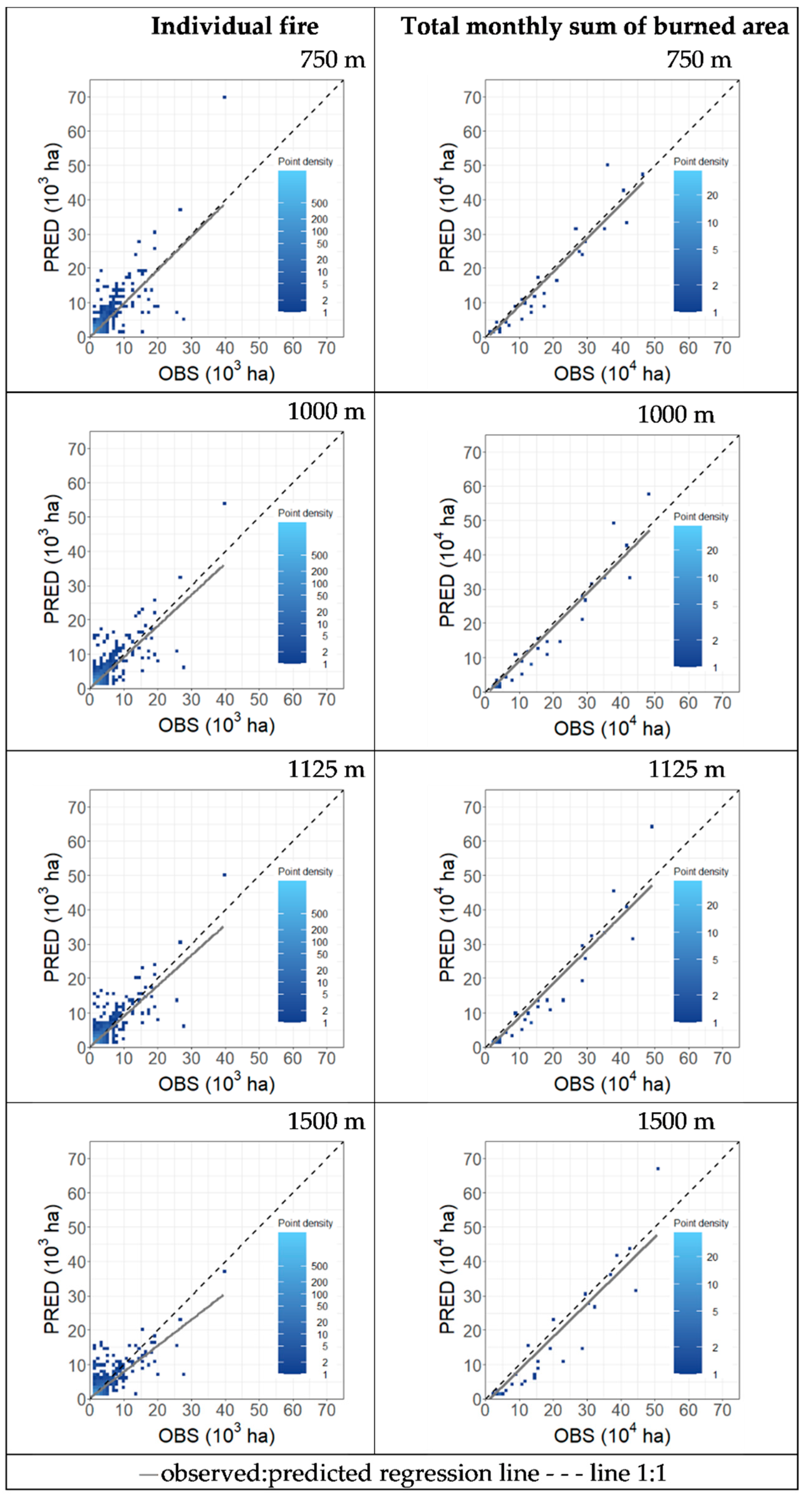
Figure 1. Map of study area considering National Institute of Geography and Statistics (INEGI) Land-Use Map Series VI (2014), 1:250,000. Forest areas are shown in green, agricultural areas in grey, human settlements in black, water bodies in pale blue. Detections of MODIS and Visible Infrared Imaging Radiometer (VIIRS) active fires from 2012 to 2018 in forest areas are shown in red. The location of detailed window Figures 4–8 are shown in turquoise, with the corresponding figure number in black.
Remotesensing 12 02061 g001
Figure 2. Predicted burned area, utilizing Equation (1), from aggregation of active fires at 750, 1000, 1125 and 1500 m against observed burned area from MCD64A1 for individual perimeters (left figures) and for total sum of burned area (right figures). PRED: predicted burned area (ha); OBS: observed MCD64A1 burned area (ha); dotted black line represents the 1:1 line and solid gray line represents the observed and predicted correlation regression line. Point density is shown in a blue gradient, representing the number or observations by each plot square division. Plot divisions, of 103 and 104 ha for individual and total burned area, respectively, are shown in grey.
Remotesensing 12 02061 g002
Figure 3. Monthly evolution from 2012 to 2018 of observed (MCD64A1) and predicted total burned area with an aggregation distance of 1125 m. PRED: predicted area in solid black line (units in hectares); OBS: observed area in dotted gray line (units in hectares).
Remotesensing 12 02061 g003
Figure 4. Examples of burned area from selected fire perimeters from May 2012, mapped using active fire data at different aggregation distances 750 m (a,e); 1000 m (b,f); 1125 m (c,g) and 1500 m (d,h) and MCD64A1 burned areas. Monthly active fire detections are shown in red points, predicted area in yellow, MCD64A1 burned area is shown in black and the agreement between predicted and observed area is shown in blue.
Remotesensing 12 02061 g004
Figure 5. Examples of aggregated active fires perimeter and MCD64A1 burned area at different aggregation distances for selected fires occurring in May 2018 (ad) and April 2017 (ef). Daily active fire detections are shown in color multiband from green to red, predicted area is shown in solid red line and MCD64A1 burned area is shown in solid black line. Numbers in squares show the corresponding burned area (ha) for both the MCD64A1 (black) and active fire aggregated (red) fire perimeters.
Remotesensing 12 02061 g005
Figure 6. Examples of errors of aggregation of active fires with 1500 m (bd) and 1125 m (a) aggregation distances. Selected examples correspond to May 2012 (a,b), June 2013 (c) and April 2012 (d). Monthly active fire detections are shown in red points, predicted area in yellow, the MCD64A1 burned area is shown in black and the agreement between predicted and observed area is shown in blue.
Remotesensing 12 02061 g006
Figure 7. Comparison of MCD64A1 burned area (BA) and aggregated active fire perimeters (AGAF) (at 1500 m,) using a field calibrated Sentinel S2 fire perimeter as reference data for selected 2019 fires in Santiago de Bayacora (a) and Tepehuanes (b) in Durango, NW Mexico. Agreement of both BA and AGAF with reference Sentinel perimeter is shown in black. Omission and commission errors for BA only (i.e., correctly detected by AGAF but not by MCD64A1 BA) are shown in green and red, respectively. Omission and commission errors for AGAF only (correctly detected by BA) are shown in blue and brown, respectively. Areas with omission and commission errors for both BA and AGAF are shown in purple and orange, respectively.
Remotesensing 12 02061 g007
Figure 8. Selected example of aggregated active fires perimeters showing the daily fire progression at 1500 m of aggregation distance. Daily fire progression and daily (April 2017) active fire detections are shown in color multiband from green to red, daily fire perimeters are shown in dotted black lines and the total fire perimeter is shown in solid red line.
Remotesensing 12 02061 g008
Table 1. Coefficients and goodness-of-fit statistics of the best models for predicting burned area by aggregation distance.
Agg. Dist. (m)Individual FireTotal Monthly Sum of Burned Area
Coefficient Goodness of FitCoefficientGoodness of Fit
aR2RMSE (ha)bias (ha)aR2RMSE (ha)bias (ha)
7501.7313(±0.0531)0.411368651.2240(±0.0308)0.9428,7998625
10001.2657(±0.0277)0.501231180.7510(±0.0186)0.9429,4069851
11251.1355(±0.0223)0.541185−90.6060(±0.0178)0.9234,91712381
15000.8150(±0.0158)0.411315−550.3268(±0.0110)0.8940,54014837
Where: Agg. Dist.: aggregation distance (units in meters); Coefficient a: is the parameter estimated by the adjusted function (Equation (1)) for the prediction of burned area from the aggregation of active fires (standard coefficient error in parentheses); R2: coefficient of determination; RMSE: root mean square error (units in ha); bias: model bias (units in ha).

