Single-Pass Soil Moisture Retrievals Using GNSS-R: Lessons Learned


1
CommSensLab-UPC, Department of Signal Theory and Communications, UPC BarcelonaTech, c/Jordi Girona 1-3, 08034 Barcelona, Spain
2
Institut d’Estudis Espacials de Catalunya-IEEC/CTE-UPC, Gran Capità, 2-4, Edifici Nexus, despatx 201, 08034 Barcelona, Spain
3
Department of Physics, UPC BarcelonaTech, 1-3 c/Jordi Girona, 08034 Barcelona, Spain
4
Institut Cartogràfic i Geològic de Catalunya, Parc de Montjuïc, 08038 Barcelona, Spain
*
Author to whom correspondence should be addressed.
Remote Sens. 2020, 12(12), 2064; https://0-doi-org.brum.beds.ac.uk/10.3390/rs12122064
Submission received: 5 May 2020
/
Revised: 20 June 2020
/
Accepted: 22 June 2020
/
Published: 26 June 2020
(This article belongs to the Special Issue Applications of GNSS Reflectometry for Earth Observation)
Abstract
:In this paper, an algorithm to retrieve surface soil moisture from GNSS-R (Global Navigaton Satellite System Reflectometry) observations is presented. Surface roughness and vegetation effects are found to be the most critical ones to be corrected. On one side, the NASA SMAP (Soil Moisture Active and Passive) correction for vegetation opacity (multiplied by two to account for the descending and ascending passes) seems too high. Surface roughness effects cannot be compensated using in situ measurements, as they are not representative. An ad hoc correction for surface roughness, including the dependence with the incidence angle, and the actual reflectivity value is needed. With this correction, reasonable surface soil moisture values are obtained up to approximately a 30° incidence angle, beyond which the GNSS-R retrieved surface soil moisture spreads significantly.
1. Introduction
The first evidence of soil moisture (SM) signatures in GPS reflected signals date back to 1996 [1]. Exploiting this technique, accurate soil moisture retrievals were successfully conducted using ground-based instruments using the so-called “interference pattern technique” (IPT) in which the direct and reflected signals are collected simultaneously by the receiving antenna, creating fringes in the received power as navigation satellites elevation varies over time. This technique can be applied using geodetic zenith-looking right-hand circularly polarized (RHCP) antennas [2], and the reflections are collected at low elevation angles for which the reflected signal is also RHCP; or it can be applied using linearly polarized (vertical, or vertical and horizontal) antennas pointing to the horizon [3,4] which allows collecting reflected signals over a much wider range of elevation angles. The latter technique also allows inferring vegetation height, and with two linear polarizations, surface roughness effects can be corrected. However, none of these techniques can be applied to airborne or spaceborne instruments.
Retrieving soil moisture from airborne and spaceborne instruments can only be performed using the reflected signal power, which requires on the instrument side the compensation of platform attitude impact on the antenna pattern, receiver’s noise… and on the target side the compensation of surface roughness (small scale as opposed to topography or large scale), and vegetation effects (both attenuation and possibly scattering). So far, two main approaches have been presented in the literature: using a change detection approach by looking to a time-series of GNSS-R data, or attempting a single-pass retrieval.
The time-series approach [5,6,7] has been able to produce operationally a soil moisture product using NASA CYGNSS (Cyclone GNSS) mission data [8]. The main advantages of the time-series approach are that assuming surface roughness and vegetation effects are constant within a grid cell (36 km in [8]), and the change in the observed reflectivity is only due to the change in the soil moisture. The main drawbacks are the difficulty to really achieve collocated GNSS-R observations over time as in the case of land, GNSS reflections exhibit a very high spatial resolution (several hundreds of meters even from space, since the spatial resolution is given by the size of the first Fresnel zone [9]), the implicit assumption of the temporal coherence of data (i.e., surface roughness or vegetation can change), and the strong non-linearities of the sensitivity of GNSS-R observables to soil moisture, which is very noticeable at low soil moisture values (Figure 1). To overcome this, in [8], an ad hoc calibration had to be performed as “the product was developed by calibrating CYGNSS reflectivity observations to soil moisture retrievals from NASA’s Soil Moisture Active Passive (SMAP) mission”.
On the other hand, single pass retrievals [10,11,12,13,14] could provide a faster revisit time, as SM maps could be generated in just one pass, provided that the instrument is accurately calibrated, and suitable ancillary data are used to compensate for surface roughness and vegetation effects without tuning the algorithm for each pixel. In [10,11], the sensitivity to soil moisture was investigated, together with a first attempt to compensate for vegetation effects using the Normalized Differential Vegetation Index (NDVI). Surface topography, spatial scales, and some subsurface “artifacts” were already reported using spaceborne data from the UK TechDemoSat-1 (TDS-1) data. Using airborne data, in [12], the sensitivity to soil moisture was studied, as well as vegetation effects, which were parameterized in terms of the Leaf Area Index (LAI) and a single scattering albedo. More recently [13], IceSat-2 data have been proposed to correct for surface roughness effects and NASA SMAP data to correct for surface roughness and vegetation optical depth (VOD) effects in the Fresnel reflection coefficients at incidence angles smaller than 35°. Even, more recently, Machine Learning techniques have been applied [14].
Despite the encouraging results of these previous works, to the authors’ knowledge, the correction of surface roughness and vegetation effects are not yet properly understood so as to perform an accurate soil moisture retrieval. In this work, the goodness of these corrections are analyzed using Sentinel-2 satellite data; GNSS-R, L-band microwave radiometry, VNIR (visible and near-infrared) hyperspectral and TIR (thermal infrared) airborne data, as well as in situ surface roughness, soil type, and soil moisture samples aiming at performing single-pass surface soil moisture (SM) retrievals using GNSS-R observations.
In order to address the above questions, an incremental approach was followed. First, based on our previous experience, very different sensitivities to soil moisture were encountered, from as high as 38 dB/100% for bare dry soils [10,15] to a more moderate approximately 9 dB/100% at global scale [11]. This large variability has to be understood first in order to properly model the sensitivity to soil moisture in the retrieval algorithm.
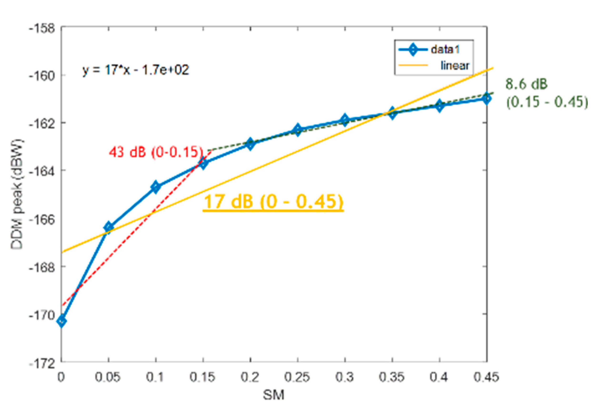
As it can be appreciated in Figure 1, computed using a comprehensive GNSS-R simulator [16], assuming a flat soil surface and no vegetation, the variation of the peak of the DDM (Delay and Doppler Map) with respect to SM is highly non-linear. Depending on the range of soil moisture values encountered in the field experiments, different slopes can be found if a linear approximation is assumed to compute the sensitivity. For example, in the range 0 to 0.15 m3/m3, the sensitivity is as high as 43 dB/100%, while in the range 0.15 to 0.45 m3/m3, the sensitivity is much lower 8.6 dB/100%, and if the whole dynamic range is considered 0 to 0.45 m3/m3, the sensitivity is 17 dB/100%.
Actually, these values demonstrate that a linearized (in dB) dependence ΔΓ/ΔSM is not valid for the whole range of SM values, and it cannot be used in SM retrieval algorithms. In addition, time-series algorithms based on the detection of reflectivity changes must also include this non-linearity as depending on the actual SM value, a given reflectivity change will correspond to different soil moisture change.
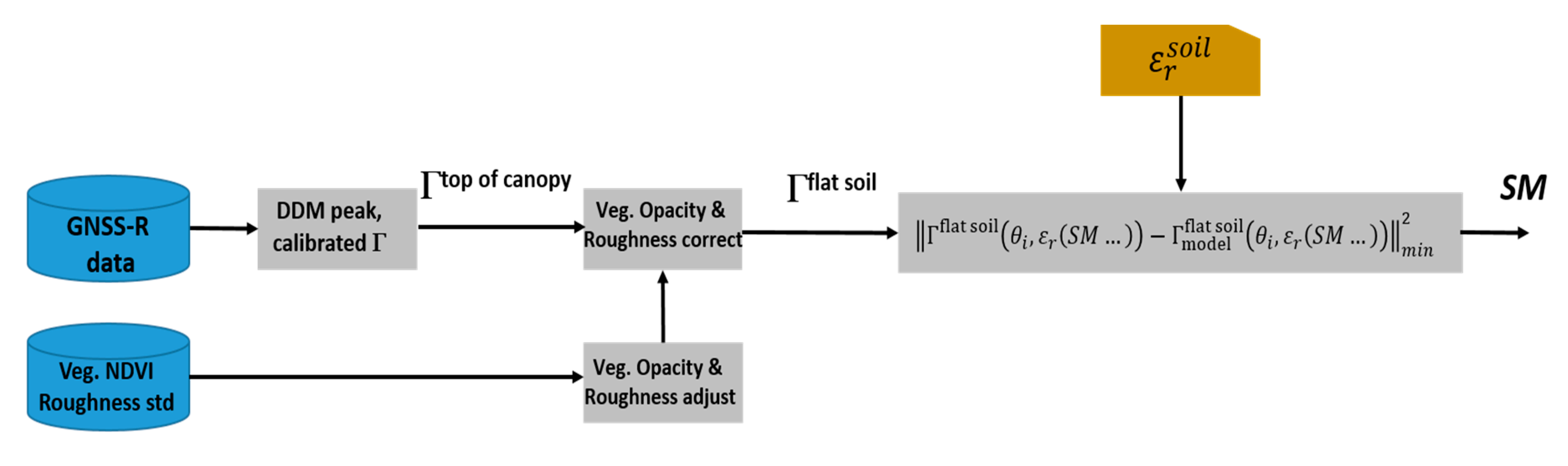
Second, the retrieval algorithm from GNSS-R observations (airborne and/or spaceborne) proceeds as follows:
- From the peak of the DDM (direct and reflected signals), and assuming that the scattered signal has a dominant coherent component, the calibrated reflection coefficient is computed taking into account the antenna pattern gains in the directions where the signals are collected, and the distances from the transmitter to the receiver, and from the transmitter to the specular reflection point plus from the specular reflection point to the receiver.
- Then, following an approach similar to the Single Channel Algorithm in SMAP [17], or in [10,12], but neglecting the single scattering albedo (ω = 0), the computed reflectivity is compensated for surface roughness (h) and vegetation effects (τ: vegetation optical depth, or VOD), in order to derive the flat surface reflectivity:
- 3.
- Then, considering the variation of the SM in the dielectric constant model for soil (among other variables, such as the clay fraction and physical temperature…), the soil moisture value can be in principle estimated through a minimization process.
The volumetric SM retrieval process is sketched in Figure 2.
At this stage, it is important to remind that in SMAP, there are three main soil moisture retrieval algorithms using microwave radiometer data: the Single Channel Algorithm (SCA), which uses the brightness temperature observations at either horizontal or vertical polarizations, and a vegetation climatology to retrieve soil moisture; and the Dual Channel Algorithm (DCA), which uses the brightness temperature observations at both horizontal and vertical polarizations, while inferring vegetation parameters as well. SMAP also uses static (climatologic) ancillary data such as soil texture and land cover class. The SCA using the brightness temperature at vertical polarization is the current baseline algorithm for SMAP level 2 soil moisture products. A recent study [20] shows that “while the DCA has its lowest unbiased root man squared error (ubRMSE) and highest R2 when ω is non-zero, the SCA have their lowest ubRMSE and highest R2 when ω = 0, and the dry bias of all algorithms increases as ω increases. Errors in soil texture are not significant, but soil surface roughness should not be static and have a higher overall value.”
When in point 2 above, it is stated that an algorithm similar to the SMAP SCA is used (with ω = 0 as found in [20]), the authors refer to the functional relationships used to account for surface roughness and vegetation effects (Equation (1)), but not to the use of SMAP climatology and ancillary data. Actually, in situ, aiborne and satellite data were acquired to parameterize the vegetation and surface roughness effects, as described in Section 2.
The rest of this work is organized as follows: Section 2 describes an airborne field experiment that was conducted to assess the SM retrieval capabilities of GNSS-R. Section 3 shows the results of the SM retrieval algorithm performance and the limitations of the surface roughness and vegetation corrections. In Section 4, additional considerations for SM retival approaches are discussed. Finally, Section 5 summarizes the main conclusions of this study.
2. Methodology: Field Experiment Description
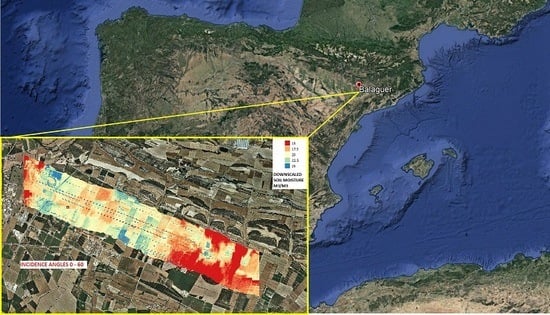
In 2017, a first airborne flight was conducted in the Tremp area (42.2°N, 0.89°E) of Lleida, Spain. The area was selected because of the availability of soil moisture stations for validation purposes. However, topography effects and the strong wind gusts affected the aircraft trajectory and attitude and did not allow for conducting the SM retrievals successfully. A second airborne campaign was conducted on October 22nd, 2018, in a flatter agricultural region around Balaguer (41.9°N, 0.80°E), Lleida, Spain (Figure 3). In situ and satellite data were acquired to complement the airborne data and allow the estimation of the surface roughness and vegetation optical depth, necessary to perform the vegetation corrections. The acquired data and the sensors are presented below.
2.1. Airborne Instrumentation and Configuration
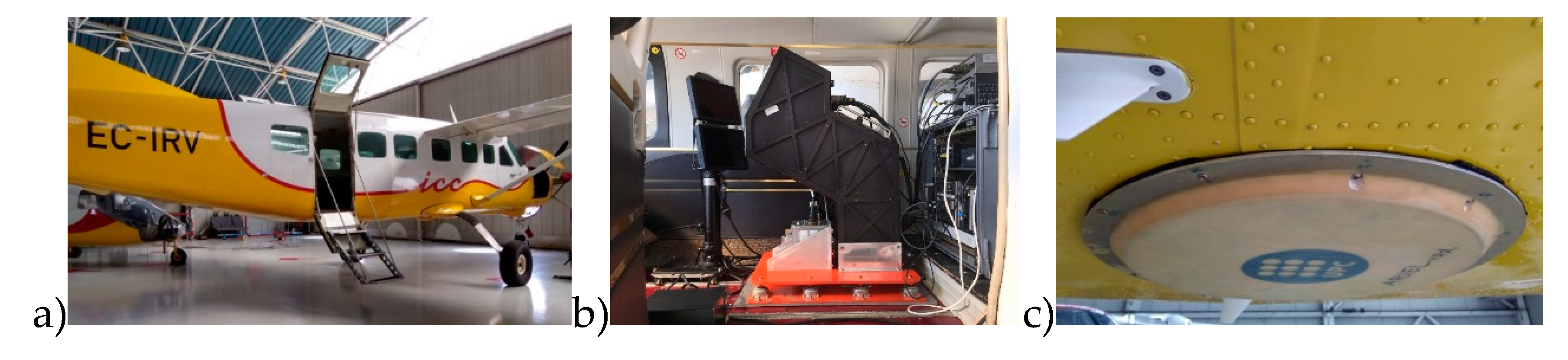
The plane used was a CESSNA Caravan (Figure 4a) from the Institut Cartogràfic i Geològic de Catalunya, with an autonomy of 4 h. The flight height was 1200 m. The instrumentation used was the following:
- CORTO (COmpact Reflectometer for Terrain Observations) is a miniature version of the LARGO [25] reflectometer at L1 GPS bands developed by the Universitat Politècnica de Catalunya. It performs the correlations between the direct and the reflected GPS signals and outputs reflectivity.
The APPLANIX [26] Inertial Navigation System (INS) on-board is a precise GNSS receiver + IMU (Inertial Measurement Unit) System that was used to geo-locate the data acquired and to perform the geometric correction on the images.
In order to receive the GPS signal for the GNSS-R instrument, there are two antennas: an RHCP up-looking GPS antenna already installed on the aircraft for navigation purposes and a LHCP down-looking one that covered the L1/L2 GPS bands. To avoid picking the direct signal through a surface wave propagating around the plane fuselage, a choke ring antenna with a carefully designed mounting was employed. The antenna radiation pattern in that configuration was measured in the UPC anechoic chamber [27] using a dummy of the bottom part of the fuselage.
2.2. Vegetation Optical Depth (VOD) Estimation from Normalized Differential Vegetation Index (NDVI)
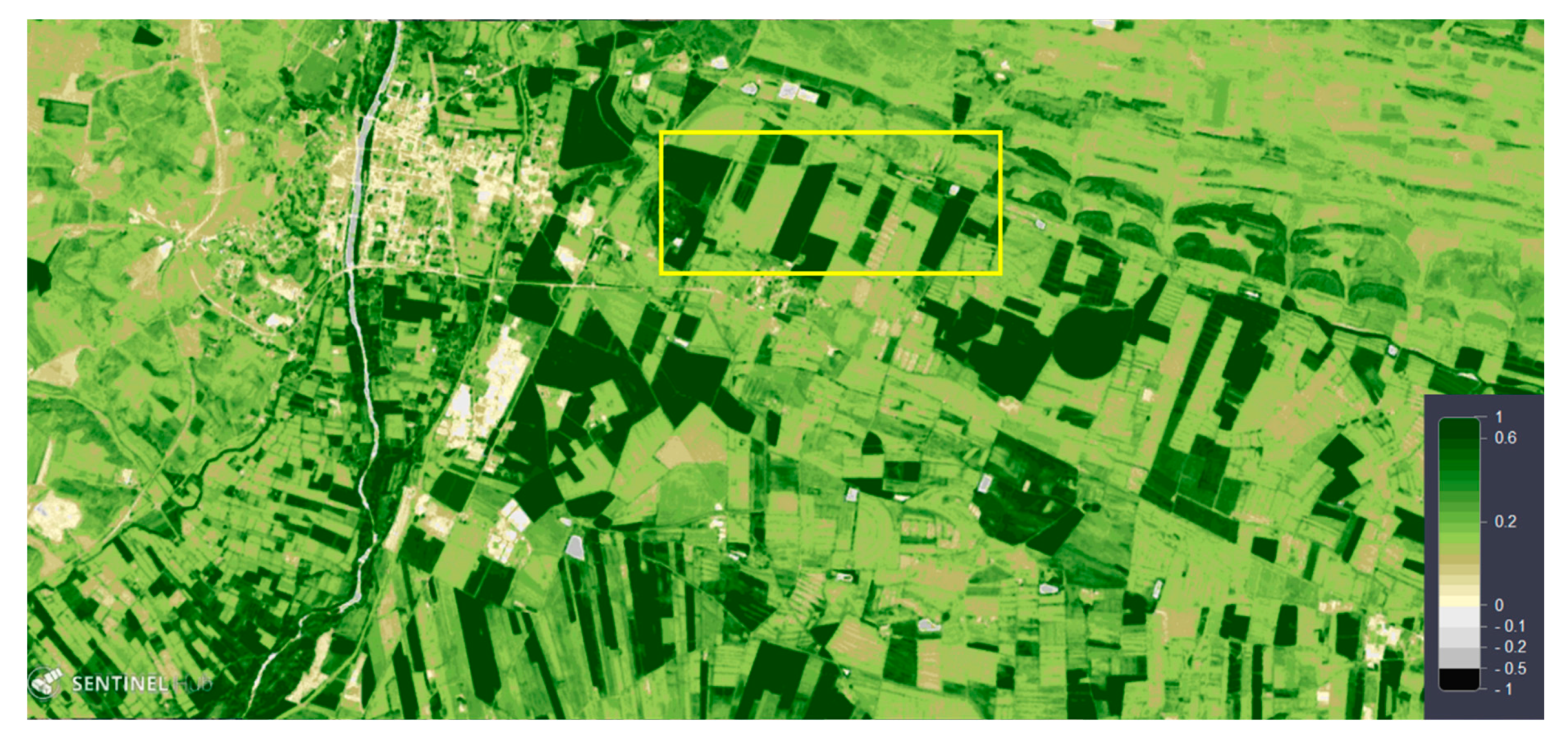
VOD is needed to compensate for the vegetation effects (Equation (1)). At the L-band, and taking into account that it is an agricultural area, with some trees, but no dense forests, the SMAP approach can be in principle used [10,12,13]. High-resolution (0.8 m) NDVI was computed from AISA data. The Sentinel-2 L1C NVDI product corresponding to Octobr 23rd, 2018 was also downloaded from the Sentinel Hub [28] (Figure 5). The VOD (τ) can be computed as:
where b is a proportionality constant that depends on the vegetation structure and the frequency, and VWC is the vegetation water content, which can be calculated using the following relationship:
where the NDVI is given by the ratio of the difference and the sum of the reflectivities in the near infrared (NIR) and the red:
The Stem Factor in Equation (3) is the product of the average vegetation height of a land cover class and the ratio of sapwood area to leaf area [17]. Sample values of b, StemFactor, and h are given in Table 3 of [17] for the land use of each observation according to the cadaster, and these are confirmed by in situ observations.
At this stage, it is important to highlight two potential error sources in these parameterizations:
- that the value of the b parameter directly determined at the satellite scale “is nearly identical to what was proposed for crops in the ESA SMOS (Soil Moisture and Ocean Salinity mission) algorithm, but half as large as what is currently used by SMAP” [29], and
- the current values of the h parameter may be too smooth (low) for crop regions, as reported in [20] for the South Fork SMAP Core Validation Site in the Corn Belt state of Iowa.
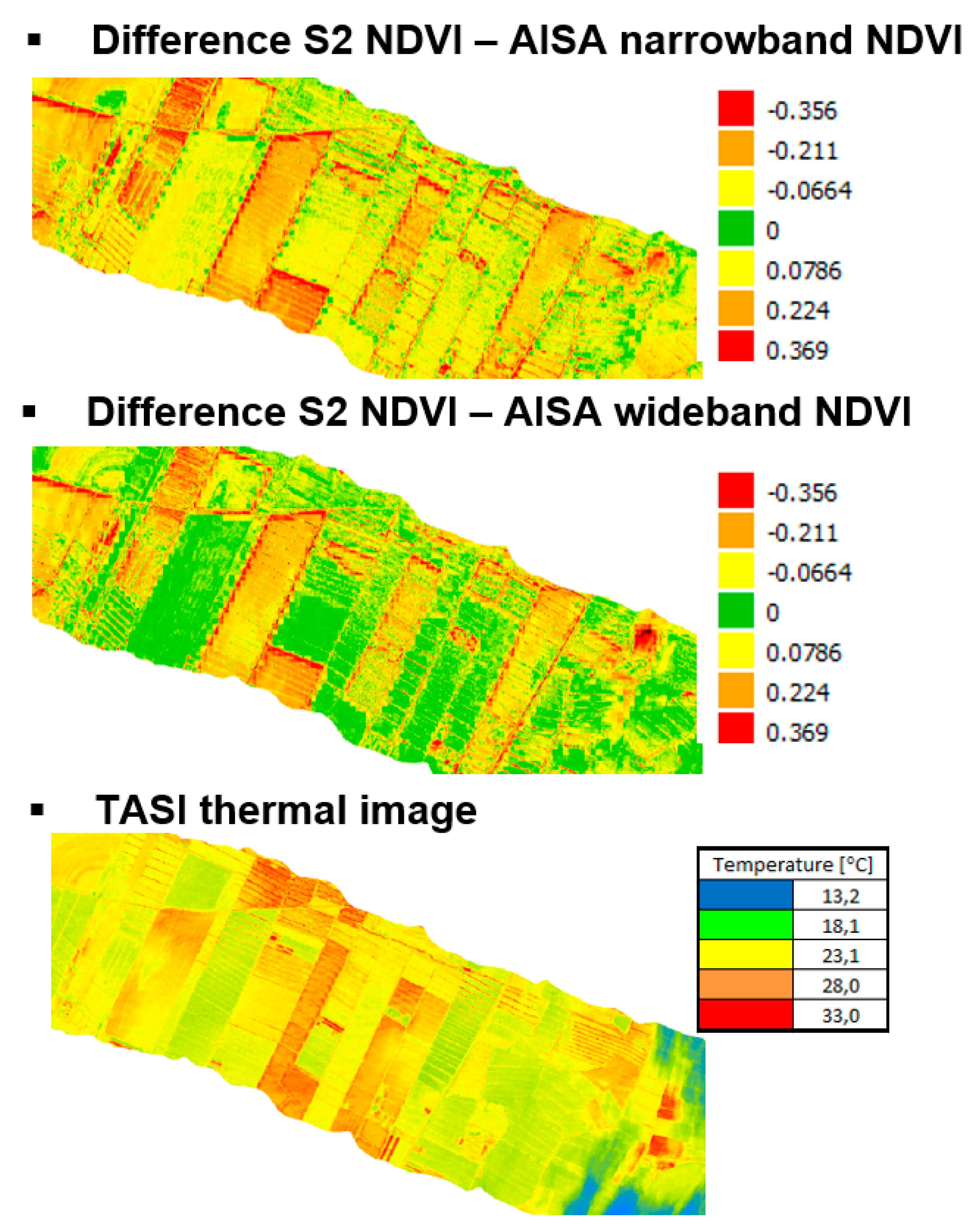
AISA NDVI was calculated using a narrowband (central wavelength) and a wideband approach, with a parametric adjustment to Sentinel-2 spectral sensitivity with respect to the wavelength.
Figure 6 shows the difference between Sentinel 2 NDVI and AISA NDVI computed either with the narrowband or wideband approaches. As it can be appreciated, the narrowband approach introduces larger errors (overestimation/underestimation) when compared to Sentinel 2 NDVI, while results with the wideband approach match much better Sentinel-2 results. As a result of the higher spatial resolution, the AISA NDVI using wideband data is used in Equations (3) and (4) to try to compensate for the vegetation effects in Equation (1). The bottom panel in Figure 6 shows the TASI thermal image in [°C]. The calibrated physical land surface temperature (LST) is lower in the bottom right corner due to the presence of clouds.
2.3. Soil Surface Roughness and Soil Moisture
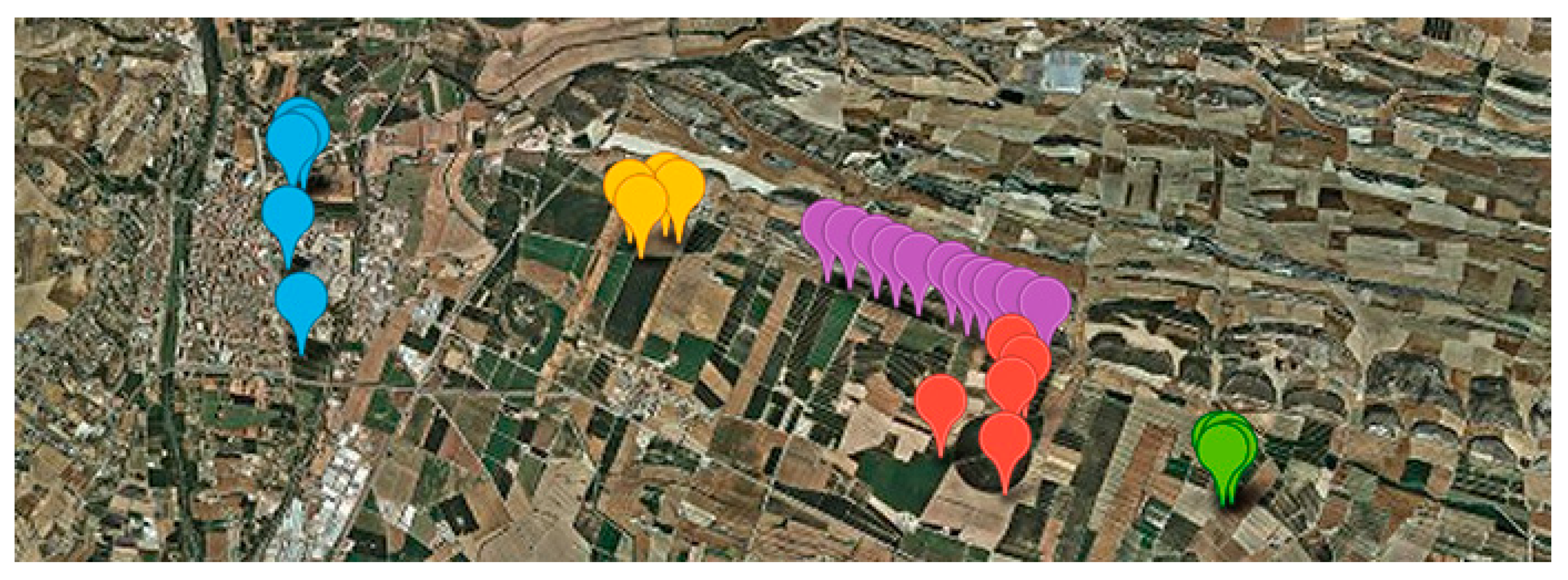
A field campaign to validate the land use and to perform the surface roughness, soil sampling, and in situ soil moisture measurements was performed the same day as the airborne campaign. Before the experiment, the Hydrogeology and Soils Unit of the Catalan Institute of Cartography and Geology (ICGC) studied the region and selected 5 different areas representative of the different agricultural activities encountered. The locations of the 29 sampling points are indicated in Figure 7.
Soil surface roughness was measured with a laser profiler based on the Leica Disto Pro4a laser distance meter, with millimetric precision, in 10 mm steps. Soil Moisture samples were acquired with a Theta Probe sensor, acquiring at least 3 samples per “sampling point” and computing the median value. Then, soil samples were analyzed in the laboratories of the IRTA (Instituto de Investigación y Tecnología Agroalimentaria)/Lleida University facilities and used for calibration of the Theta Probe sensor.
The largest problem with the “effective” surface soil roughness is its difficult estimation, as it depends on numerous additional factors such as the soil composition, the agricultural activity, the state of the crops, etc. [30]. Moreover, this seasonal dependency only correlates with similar fields.
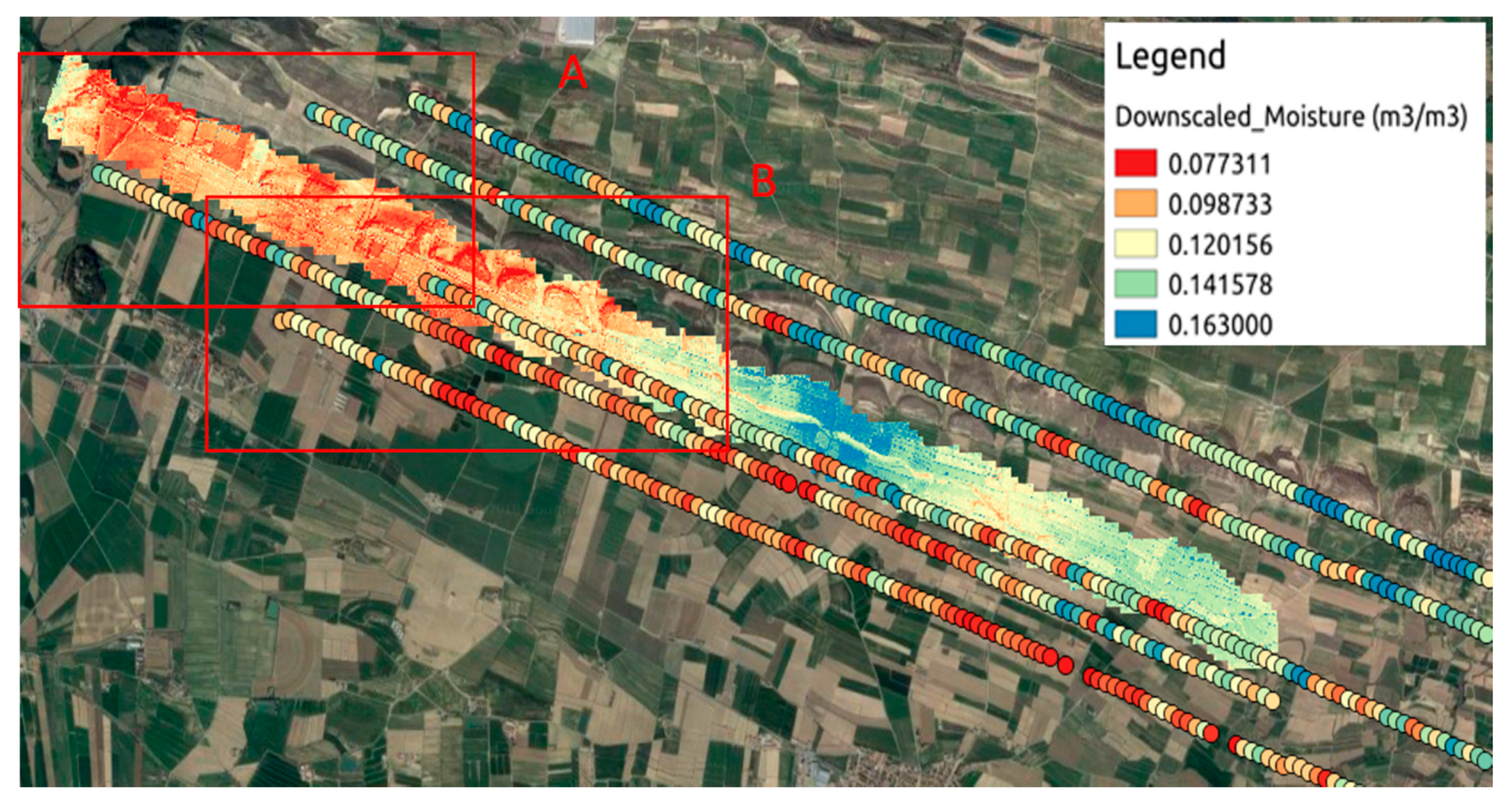
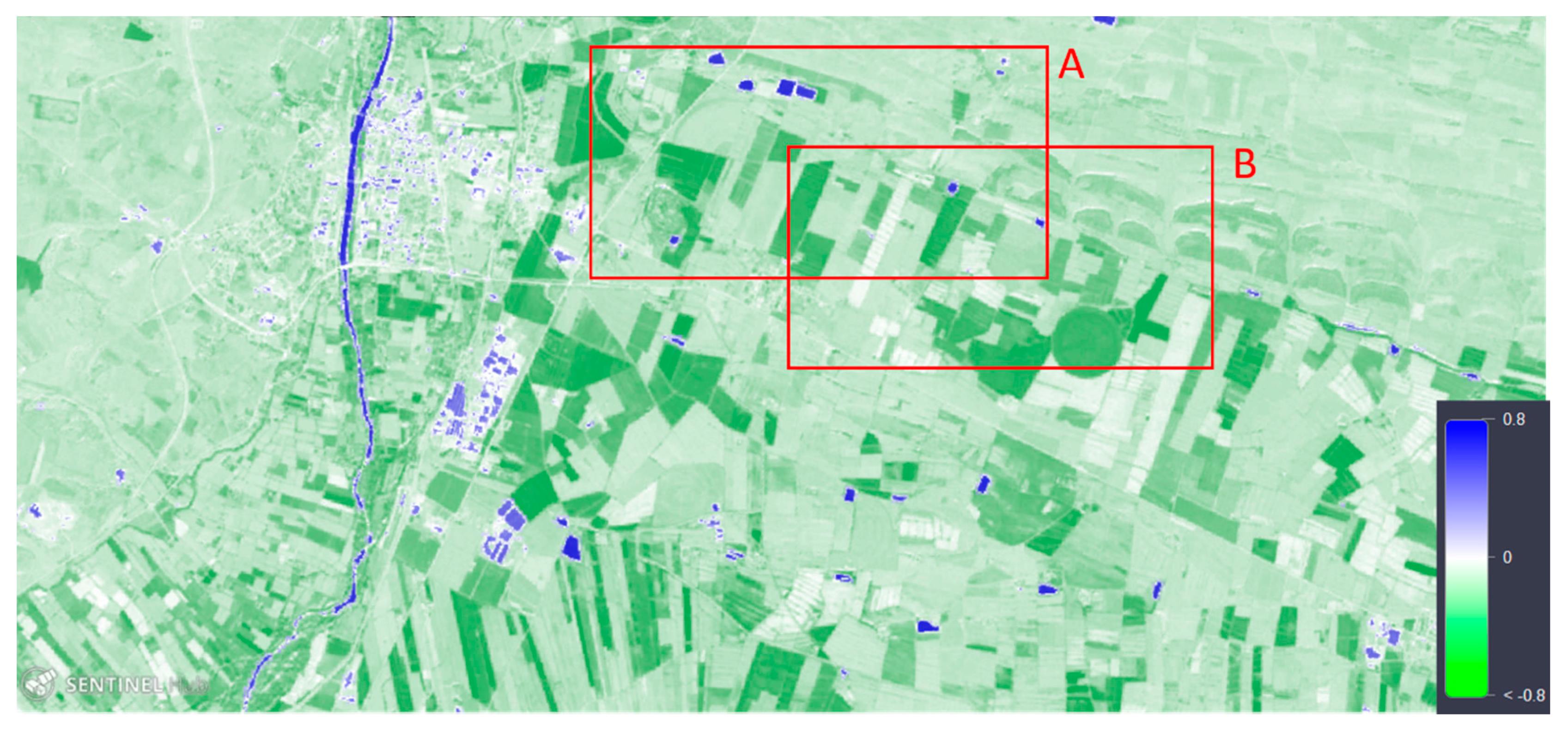
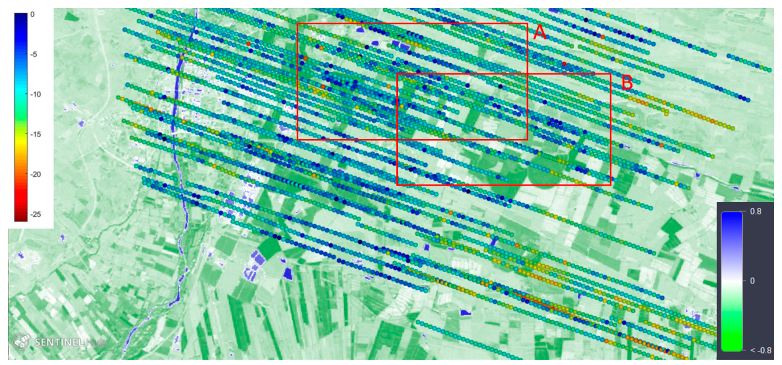
In the aircraft, the ARIEL L-band radiometer was flown to provide a complete 0.8 m resolution SM map (Figure 8) using a downscaling algorithm that combines TASI and AISA data [31,32]. This algorithm has been validated [33] extensively, and in this experiment, the root mean square error (rmse) and bias were approximately 0.06 m3/m3, and −0.01 m3/m3 with respect to the in situ soil moisture measurements. As a qualitative validation, Figure 9 shows the Sentinel 2 Normalized Difference Water Index (NDWI) for October 23rd, 2018. Similarly to the NDVI, the NDWI index uses the green and near infrared bands (bands 3 and 8), and because of the strong absorbability and low radiation in the range from visible to infrared wavelengths, it is most appropriate for water body mapping, to assess the surface soil moisture and vegetation hydric stress. Figure 10 shows the GNSS-Reflectivities overlaid with the Sentinel-2 L1C NDWI.
3. GNSS-R Soil Moisture Retrieval: Results
In this section, the resulting SM maps are assessed for different corrections applied. The results are shown over an ortho-photo of the Region Of Interest (ROI). There are two layers of data: ARIEL downscaled SM (0.8 m spatial resolution), and overlapped samples of the GNSS-R retrieved SM at the same resolution. The ARIEL SM retrievals are used to validate the estimations of GNSS-R SM retrievals.
3.1. In Situ Surface Roughness Correction
In this first attempt, the measured surface roughness with the laser profiler was used to compute the roughness parameter required in Equations (1) and (11) of [18] from the soil surface roughness (σ):
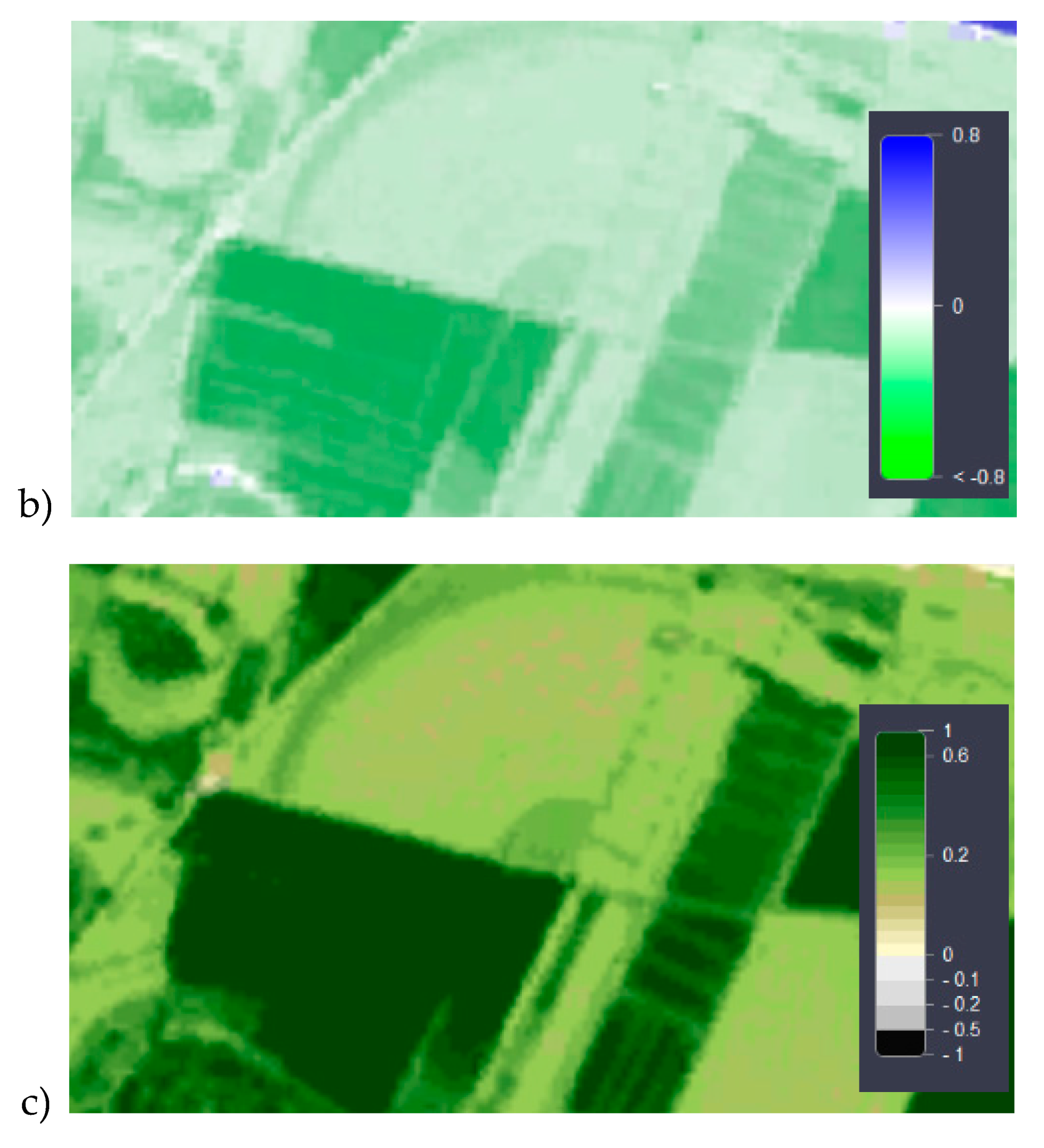
Due to the limited accuracy and coarse sampling of the soil surface roughness, the results show a large disparity between the ARIEL and the GNSS-R SM retrievals. As it can be appreciated in Figure 11a, for a single track of GNSS-R reflections over a relatively flat area (no topography), the retrieved SM values are highly variable with the incidence angle (see alternating SM retrievals between approximately 0.14 and 0.27), and these are quite different than the ARIEL downscaled SM ~0.21, although on average, it is relatively close (e.g., 0.21 ≈ (0.14 + 0.27)/2). Apart from the different scales (0.8 m versus 10 m), note the high visual correlation between Figure 11a, ARIEL downscaled soil moisture, and Figure 11b Sentinel 2 L1C NDWI.
3.2. Ad Hoc Soil Surface Roughness Correction
The lack of success in this first SM retrieval approach with the in situ measured soil surface roughness led us to consider that the surface roughness correction applied was not appropriate, either in the value of the h parameter, and/or the power of the cosine function (n = 0, 1, or 2) in Equation (1). As discussed in page 35 of [17], the cos2θ term is sometimes changed to cosθ or even dropped completely to avoid overcorrecting for roughness.
To derive the “correct” surface roughness correction, the same procedure was applied, but adding an ad hoc surface roughness correction term h, as in , so that the retrieved GNSS-R SM values match as close as possible the ARIEL-derived ones. The step-by-step procedure is described below:
- Compensation of vegetation effects (Equations (1)–(4)).
- Compensation of surface roughness effects (as in Equation (1) and (2): , for n = 0, 1, and 2.
- Apply SM retrieval algorithm by minimizing the difference between the computed flat bare soil reflectivity using ARIEL-derived SM, and GNSS-R calibrated reflectivity () plus the ad hoc surface roughness compensation term (in [dB]).
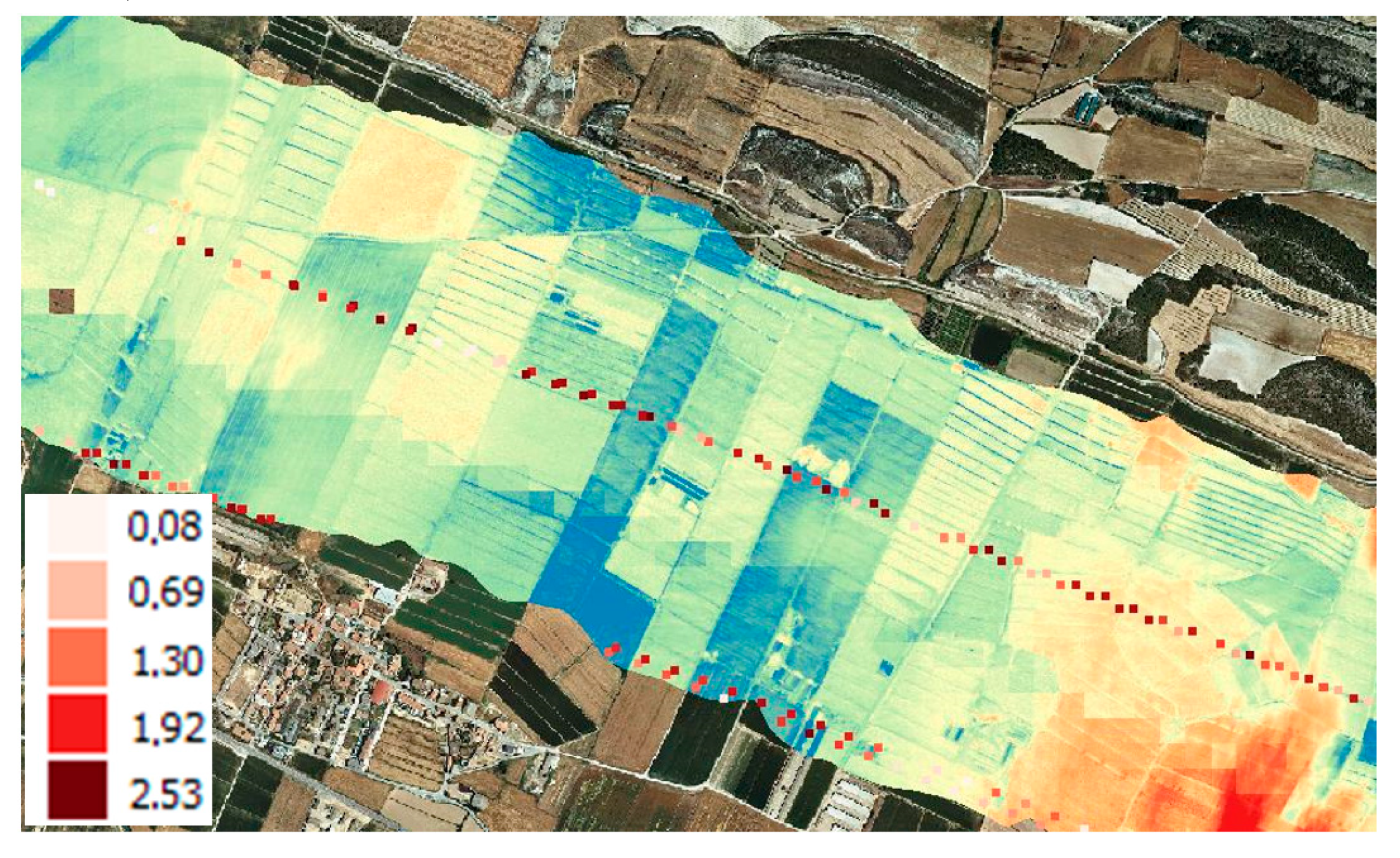
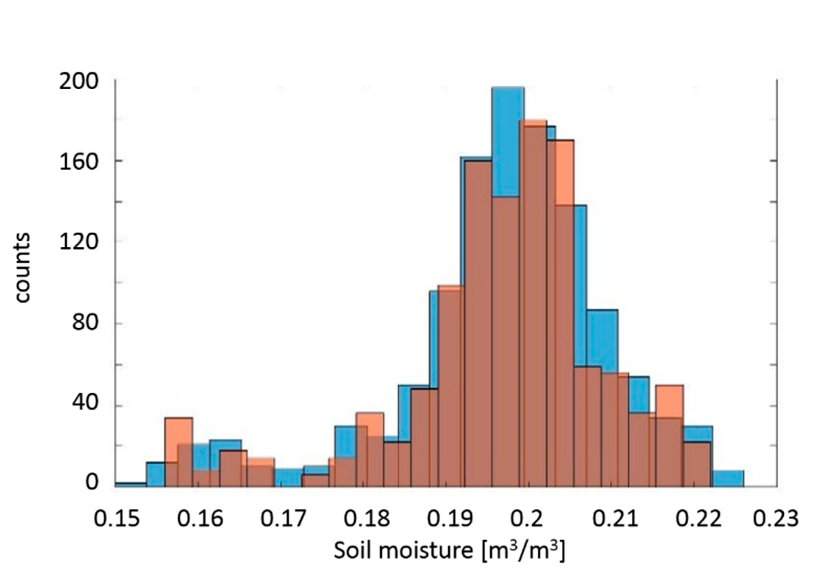
It was found that for n = 0, the scatter in the ad hoc surface roughness corrections was the smallest one obtained. For n = 2, the corrections were more exaggerated, indicating they were artificially high. Figure 12 shows the map of the computed surface roughness parameters (h). Apparently, there is no evident correlation neither with the different fields nor with the soil moisture values, although some of the largest values occur in the plots with higher humidity, but not all. In addition, as expected, by construction, the matched histograms of the SM values retrieved by downscaling ARIEL’s measurements and from CORTO’s reflectivity with the ad hoc surface roughness correction are basically the same (Figure 13), except for numerical round off errors in the surface roughness correction (0.1 dB) during the optimization process (third bullet in the above list, or the right box in the diagram in Figure 2).
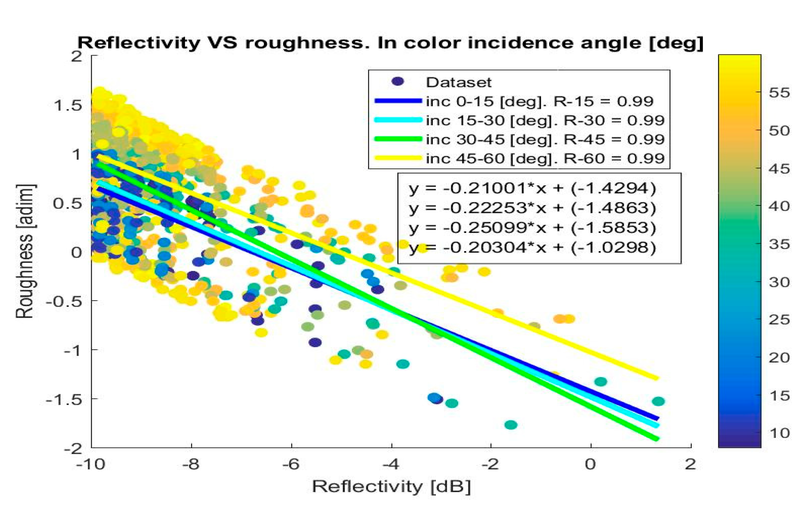
Figure 14 shows the estimated values of h (as in ). A more detailed analysis of the ad hoc surface roughness correction reveals that it increases for lower reflectivity values. This apparently has no physical meaning, and it is difficult to interpret as an instrumental error. It was also considered that it could be an imperfect estimation of the noise floor of the DDM background, which is needed in the calibration, but this does not explain why, for the same reflectivity values, the correction varies with the incidence angle, increasing for the larger ones. Additionally, negative values in h (roughness correction larger than 0 dB at low reflectivities) do not have a physical meaning, but they led us to think that actually the compensation of the vegetation effects as in Equations (1)–(4) was too high, as already shown in Figure 13 of [11]. This effect is examined in more detail in the next section.
3.3. Vegetation and Roughness Compensation for Different Incidence Angles
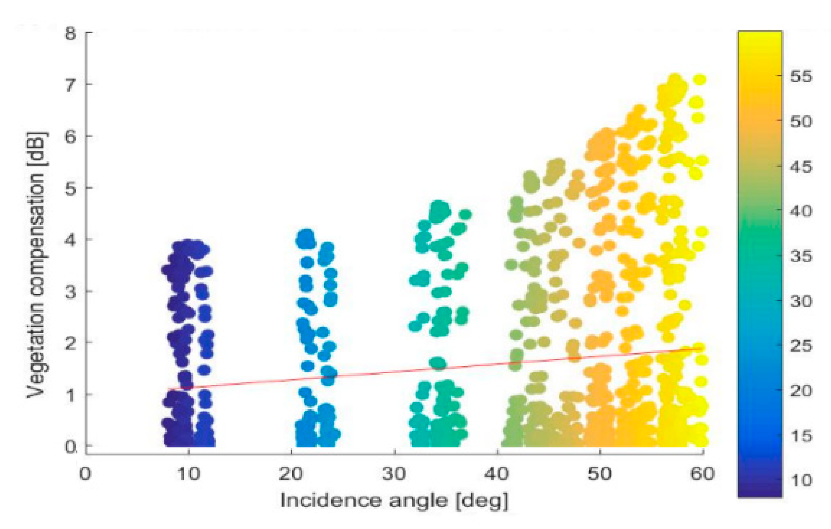
Figure 15 shows the scatter plot of the vegetation compensation [dB] (Equation (1)) with respect to the incidence angle. The compensation of vegetation effects increases with incidence angle, as it has a functional dependence with (see the variation of peak values wrt. incidence angle). The compensation of the roughness effects has also a dependence on the incidence angle, but it can be modeled neither with n = 1, nor with n = 2.
Since the compensation of vegetation effects is fixed and depends on the VOD (which is calculated using the NDVI) and the incidence angle, an overcompensation of the vegetation attenuation forces the algorithm to reduce the compensation of the surface roughness component, and that is why the algorithm even finds negative surface roughness coefficients. This effect is more important for large incidence angles, and it suggests that the vegetation compensation is too high at large incidence angles, which is in agreement with [13], who found that corrections were only applicable up to approximately a 35° incidence angle.
Other sources of variability are:
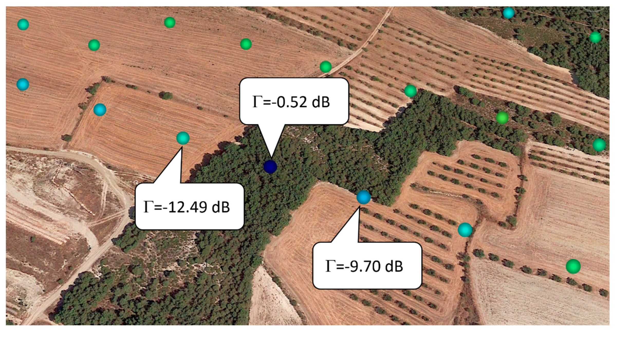
- high reflectivity values encountered in vegetated areas (trees, higher soil moisture), but from the processing point of view, require a too high attenuation compensation, leading to “corrected” flat bare reflectivity values larger than one (0 dB) in Figure 14. This is illustrated in Figure 16 by the dark blue dot over a forested area in the middle of the image, pointed by the triangle, and legend with the parameters.
- there is likely a subsurface variability of the soil moisture that is detected by GNSS-R, as there are regions in the fields where the reflectivity suddenly increases (see lines of light blue or green values in Figure 10, with some dark blue—high reflectivity—observations in the middle), while all other parameters are nearly constant.
3.4. Empirical Roughness Compensation
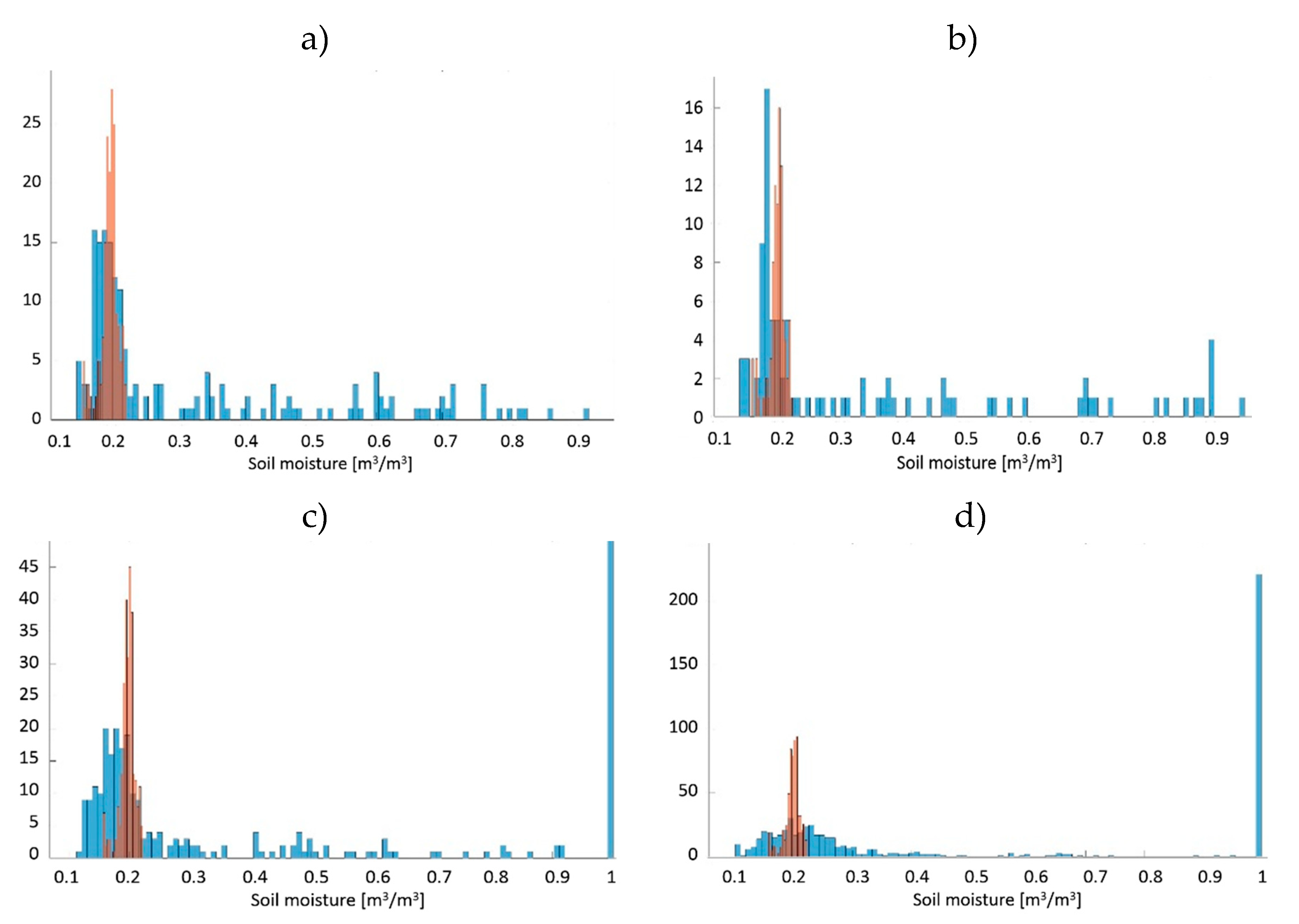
Not being satisfied with the result that accurate single-pass soil moisture retrievals were only feasible if a pixel-based ad hoc correction of the surface roughness was used, an empirical correction (1st order polynomial) for all pixels within a given range of incidence angles is attempted. The procedure is the same as in the pixel-by-pixel approach described before, but now computing the minimum root mean squared error (RMSE) for all pixels simultaneously. Figure 17 shows the histograms of the ARIEL-retrieved SM values, and the GNSS-R retrieved ones using a generic empirical 1st order polynomial correction for all pixels within a given range of incidence angles. As it can be appreciated, except for a few outliers, the matching is quite reasonable up to approximately a 30° incidence angle, and beyond that, the retrieved histograms widen and GNSS-R derived SM values tend to widen and scatter significantly (sensitivity to SM decreases, while the effect of roughness is still non-negligible). This result is also in agreement with [13] where corrections were only applicable up to an approximately 35° incidence angle.
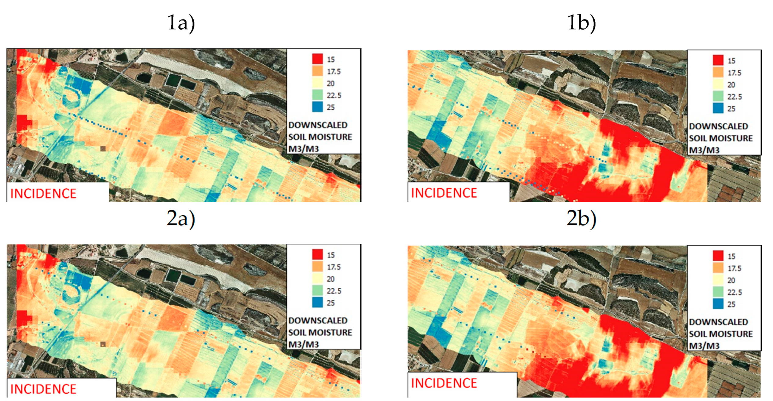
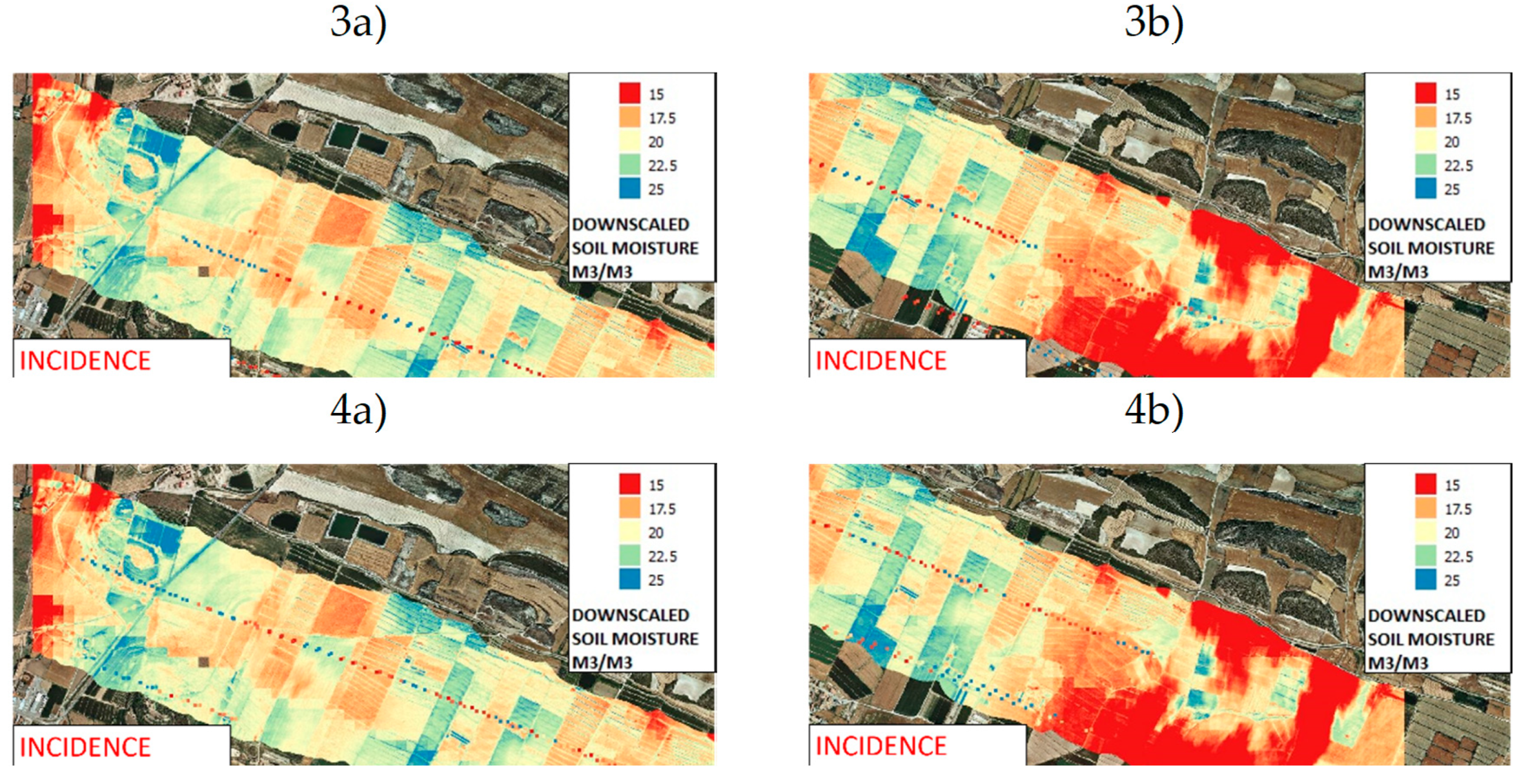
Figure 18 shows the soil moisture maps for two regions (left and right column, corresponding to regions A and B, respectively in Figure 8, Figure 9 and Figure 10) during the flight for all ranges of incidence angles in steps of 15°. Squares correspond to GNSS-R-derived soil moisture using the generic angular-dependent roughness correction.
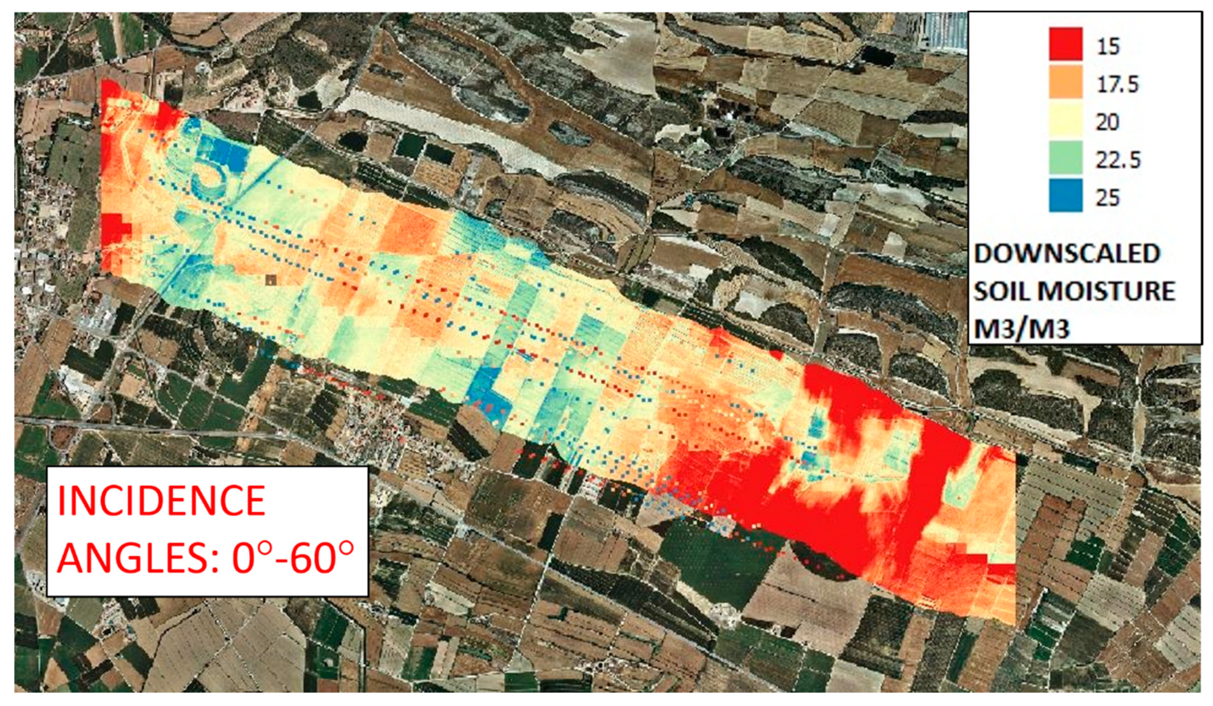
Finally, Figure 19 presents the downscaled ARIEL and GNSS-R-retrieved SM overlaid maps for all incidence angles included, showing a reasonable agreement, which degrades for increasing incidence angles.
4. Discussion
In the previous sections, it was shown that the sensitivity of the calibrated reflectivity to Soil Moisture is non-linear and varies with the Soil Moisture value (Figure 1) [16]. Linearized retrieval approaches must be cautious in order not to introduce biases and other artifacts. Soil moisture retrieval algorithms require that vegetation and surface roughness effects must be properly compensated first.
Current models adopted from L-band microwave radiometry (1.413 GHz) overcorrect vegetation effects [11], which leads to an overcorrection of the surface roughness to try to compensate for the vegetation correction. Therefore, techniques to better predict the vegetation corrections are needed, as current models adopted from L-band microwave radiometry (1.413 GHz) using a VOD estimate from the NDVI [17] seem to overestimate it, which leads to an overcompensation of the surface roughness effects to counteract them. A potential source of this discrepancy may be in the values of the b parameter, which are too high in crop regions, as recently reported in [29].
In situ measurements of the surface roughness are not suitable to predict the surface roughness parameter to be used in the compensation, as different roughness values are obtained with different techniques [34], i.e., a laser profiler with respect to mechanical profiler, and that there is an impact of the profiler length and number of independent measurements. It is also possible that the reflection is taking place effectively in the water table underground, behaving then as a much “flatter” surface than the air–soil interface. Volume scattering effects in the soil cannot be neglected, either. The use of a constant value of “h” (e.g., as in SMAP) is not suitable either, even if it is different for each field. In addition, it has been recently reported that the current values of the h parameter may be too smooth (low) for crop regions [20]. Generic surface roughness empirical corrections as a function of the range of incidence angles are also possible, leading to acceptable results: the root mean squared error between downscaled ARIEL and GNSS_R SM map is < 5%, while today’s UCAR/CU soil moisture product developed by calibrating CYGNSS reflectivity observations to soil moisture retrievals from NASA SMAP mission exhibits a median unbiased root-mean-square error (ubRMSE) of 0.049 m3/m3 [8].
5. Conclusions
Recent results [13] claim that IceSat-2 surface roughness data can be used to correct for these effects at a global scale. However, the authors of this study believe that further improvements using auxiliary data from other sensors are unlikely, as it is very difficult to match all the observations in time and space, and that they can vary over time, and techniques to infer the effective soil surface roughness parameter, if possible from the data themselves, are needed. A clear example is the estimation of the surface roughness from the GNSS-R observables [35].
Further research is also needed to explore the simultaneous use of several GNSS bands and other GNSS-R observables with variable coherent and incoherent integration times, and to include the non-linear dependence of the VOD with the above ground biomass (ABG), as shown in Supplementary Figure 4 from [36,37]. Vegetation scattering and wave depolarization have to be accounted for as well.
In the meantime, while these corrections are not improved for single pass retrievals, time-series approaches based on temporal changes of the reflectivity (e.g., [5,6,7,8]) can be applied, provided that the non-linearities of the dependence of the GNSS-R observables and the SM are properly taken into account, and self-consistency of the retrieved products is demonstrated.
The most relevant result of this study is that despite all the above limitations in the surface roughness and vegetation effects corrections, single-pass GNSS-R soil moisture values seem feasible with a reasonable error (<5%) for incidence angles up to 30°, provided that an incidence angle dependent soil surface roughness correction is applied.
Author Contributions
Conceptualization, A.C.; methodology, A.C.; software, A.C. and J.C. (Jordi Castellví); validation, A.C. and J.C. (Jordi Castellví); formal analysis, A.C.; investigation, A.C., H.P.; resources, A.C., H.P., J.C. (Jordi Corbera); data curation, J.C. (Jordi Castellví), E.A.; writing—original draft preparation, A.C.; writing—review and editing, H.P., J.C. (Jordi Corbera); visualization, A.C., J.C. (Jordi Castellví), H.P.; supervision, A.C.; project administration, A.C., J.C. (Jordi Corbera); funding acquisition, A.C., J.C. (Jordi Corbera). All authors have read and agreed to the published version of the manuscript.
Funding
This work has been funded by the Spanish MCIU and EU ERDF project (RTI2018-099008-B-C21) “Sensing with pioneering opportunistic techniques” and grant to ”CommSensLab-UPC” Excellence Research Unit Maria de Maeztu (MINECO grant MDM-2016-600), and by a Doctorat Industrial grant from ICGC.
Acknowledgments
The authors would like to thank the flight department of ICGC for the work carried out to design and implement the new sensors onboard ICGC airplane as well as the operational flight campaign
Conflicts of Interest
The authors declare no conflict of interest.
References
- Kavak, A.; Xu, G.; Vogel, W.J. GPS multipath fade measurements to determine L-band ground reflectivity properties. In Proceedings of the 20th NASA Propagation Experiment Meeting (NAPEX 20) Fairbank; Alaska, Organizer: Jet Propulsion Laboratory: Pasadena, CA, USA, 1996; pp. 257–263. [Google Scholar]
- Larson, K.M.; Braun, J.J.; Small, E.E.; Zavorotny, V.U.; Gutmann, E.D.; Bilich, A.L. GPS Multipath and Its Relation to Near-Surface Soil Moisture Content. IEEE J. Sel. Top. Appl. Earth Obs. Remote Sens. 2010, 3, 91–99. [Google Scholar] [CrossRef]
- Rodriguez-Alvarez, N.; Bosch-Lluis, X.; Camps, A.; Vall-llossera, M.; Valencia, E.; Marchan-Hernandez, J.F.; Ramos-Perez, I. Soil Moisture Retrieval Using GNSS-R Techniques: Experimental Results Over a Bare Soil Field. IEEE Trans. Geosci. Remote Sens. 2009, 47, 3616–3624. [Google Scholar] [CrossRef]
- Arroyo, A.A.; Camps, A.; Aguasca, A.; Forte, G.F.; Monerris, A.; Rüdiger, C.; Walker, J.P.; Park, H.; Pascual, D.; Onrubia, R. Dual-Polarization GNSS-R Interference Pattern Technique for Soil Moisture Mapping. IEEE J. Sel. Top. Appl. Earth Obs. Remote Sens. 2014, 7, 1533–1544. [Google Scholar] [CrossRef]
- Chew, C.; Small, E. Soil moisture sensing using spaceborne GNSS reflections: Comparison of CYGNSS reflectivity to SMAP soil moisture. Geophys. Res. Lett. 2018, 45, 4049–4057. [Google Scholar] [CrossRef] [Green Version]
- Clarizia, M.P.; Pierdicca, N.; Costantini, F.; Floury, N. Analysis of CyGNSS Data for Soil Moisture Retrieval. IEEE J. Sel. Top. Appl. Earth Obs. Remote Sens. 2019, 12, 2227–2235. [Google Scholar] [CrossRef]
- Al-Khaldi, M.M.; Johnson, J.T.; O’Brien, A.J.; Balenzano, A.; Mattia, F. Time-Series Retrieval of Soil Moisture Using CYGNSS. IEEE Trans. Geosci. Remote Sens. 2019, 57, 4322–4331. [Google Scholar] [CrossRef]
- Chew, C.; Small, E. Description of the UCAR/CU Soil Moisture Product. Remote Sens. 2020, 12, 1558. [Google Scholar] [CrossRef]
- Camps, A. Spatial Resolution in GNSS-R Under Coherent Scattering. IEEE Geosci. Remote Sens. Lett. 2020, 17, 32–36. [Google Scholar] [CrossRef]
- Camps, A.; Park, H.; Pablos, M.; Foti, G.; Gommenginger, C.P.; Liu, P.; Judge, J. Sensitivity of GNSS-R Spaceborne Observations to Soil Moisture and Vegetation. IEEE J. Sel. Top. Appl. Earth Obs. Remote Sens. 2016, 9, 4730–4742. [Google Scholar] [CrossRef] [Green Version]
- Camps, A.; Vall·llossera, M.; Park, H.; Portal, G.; Rossato, L. Sensitivity of TDS-1 GNSS-R Reflectivity to Soil Moisture: Global and Regional Differences and Impact of Different Spatial Scales. Remote Sens. 2018, 10, 1856. [Google Scholar] [CrossRef] [Green Version]
- Zribi, M.; Motte, E.; Baghdadi, N.; Baup, F.; Dayau, S.; Fanise, P.; Guyon, D.; Huc, M.; Wigneron, J.-P. Potential Applications of GNSS-R observations over agricultural areas: Results from the GLORI airborne campaign. Remote Sens. 2018, 10, 17. [Google Scholar] [CrossRef] [Green Version]
- Calabia, A.; Molina, I.; Jin, S. Soil Moisture Content from GNSS Reflectometry Using Dielectric Permittivity from Fresnel Reflection Coefficients. Remote Sens. 2020, 12, 122. [Google Scholar] [CrossRef] [Green Version]
- Jia, Y.; Jin, S.; Savi, P.; Gao, Y.; Tang, J.; Chen, Y.; Li, W. GNSS-R Soil Moisture Retrieval Based on a XGboost Machine Learning Aided Method: Performance and Validation. Remote Sens. 2019, 11, 1655. [Google Scholar] [CrossRef] [Green Version]
- Camps, A.; Forte, G.; Ramos, I.; Alonso, A.; Martinez, P.; Crespo, L.; Alcayde, A. 2012: Recent Advances in Land Monitoring Using GNSS-R Techniques, 2012 Workshop on Reflectometry Using GNSS and Other Signals of Opportunity (GNSS+R); West Lafayette: Indiana, IN, USA, 2012; pp. 1–4. [Google Scholar] [CrossRef]
- Park, H.; Camps, A.; Castellvi, J.; Muro, J. Generic Performance Simulator of Spaceborne GNSS-Reflectometer for Land Applications. IEEE J. Sel. Top. Appl. Earth Obs. Remote Sens. 2020, 13, 3179–3191. [Google Scholar] [CrossRef]
- O’Neill, P.; Bindlish, R.; Chan, S.; Njoku, E.; Jackson, T. Soil Moisture Active Passive (SMAP), Algorithm Theoretical Basis Document Level 2 & 3 Soil Moisture (Passive) Data Products. Revision D, June 6, 2018, Technical Note JPL D-66480. Available online: https://smap.jpl.nasa.gov/system/internal_resources/details/original/484_L2_SM_P_ATBD_rev_D_Jun2018.pdf (accessed on 24 May 2020).
- Choudhury, J.B.; Schmugge, T.J.; Chang, A.; Newton, R.W. Effect of surface roughness on the microwave emission from soil. J. Geophys. Res. 1979, 84, 5699–5706. [Google Scholar] [CrossRef]
- Wang, J.R. Passive microwave sensing of soil moisture content: The effects of soil bulk density and surface roughness. Remote Sens. Environ. 1983, 13, 329–344. [Google Scholar] [CrossRef]
- Walker, A.V.; Hornbuckle, B.K.; Cosh, M.H.; Prueger, J.H. Seasonal Evaluation of SMAP Soil Moisture in the U.S. Corn Belt. Remote Sens. 2019, 11, 2488. [Google Scholar] [CrossRef] [Green Version]
- AISA Technical Data. Available online: https://www.channelsystems.ca/sites/default/files/documents/aisa_products_ver1-2015.pdf (accessed on 22 April 2020).
- TASI600 Technical Data. Available online: https://itres.com/wp-content/uploads/2019/09/TASI600.pdf (accessed on 22 April 2020).
- Acevo-Herrera, R.; Aguasca, A.; Bosch-Lluis, X.; Camps, A.; Martínez-Fernández, J.; Sánchez-Martín, N.; Pérez-Gutiérrez, C. Design and First Results of an UAV-Borne L-Band Radiometer for Multiple Monitoring Purposes. Remote Sens. 2010, 2, 1662–1679. [Google Scholar] [CrossRef] [Green Version]
- ARIEL Technical Data. Available online: https://www.balamis.com/products/ (accessed on 22 April 2020).
- Sánchez, N.; Alonso-Arroyo, A.; Martínez-Fernández, J.; Piles, M.; González-Zamora, A.; Camps, A.; Vall-llosera, M. On the Synergy of Airborne GNSS-R and Landsat 8 for Soil Moisture Estimation. Remote Sens. 2015, 7, 9954–9974. [Google Scholar] [CrossRef] [Green Version]
- Applanix Web Site. Available online: https://www.applanix.com/products/posav.htm (accessed on 24 May 2020).
- UPC Anechoic Chamber. Available online: https://www.tsc.upc.edu/en/facilities/anechoic-chamber (accessed on 24 May 2020).
- Sentinel Hub-EO Browser. Available online: https://apps.sentinel-hub.com/eo-browser/ (accessed on 24 May 2020).
- Togliatti, T.K.; Hartman, T.; Walker, V.A.; Arkebaur, T.J.; Suyker, A.E.; VanLoocke, A.; Hornbuckle, B.K. Satellite L–band vegetation optical depth is directly proportional to crop water in the US Corn Belt. Remote Sens. Environ. 2019, 223, 111. [Google Scholar] [CrossRef]
- Panciera, R.; Walker, J.P.; Merlin, O. Improved Understanding of Soil Surface Roughness Parameterization for L-Band Passive Microwave Soil Moisture Retrieval. IEEE Geosci. Remote Sens. Lett. 2009, 6, 625–629. [Google Scholar] [CrossRef]
- Piles, M.; Camps, A.; Vall·llossera, M.; Corbella, I.; Panciera, R.; Rudiger, C.; Kerr, H.Y.; Walker, J. 2011: Downscaling SMOS-Derived Soil Moisture Using MODIS Visible/Infrared Data. IEEE Trans. Geosci. Remote Sens. 2011, 49, 3156–3166. [Google Scholar] [CrossRef]
- Portal, G.; Vall-llossera, M.; Piles, M.; Camps, A.; Chaparro, D.; Pablos, M.; Rossato, L. 2018: A Spatially Consistent Downscaling Approach for SMOS Using an Adaptive Moving Window. IEEE J. Sel. Top. Appl. Earth Obs. Remote Sens. 2018, 11, 1883–1894. [Google Scholar] [CrossRef]
- Pablos, M.; Piles, M.C. Gonzalez-Haro and BEC TeamBEC SMOS Land Products Description. Technical Note: BEC-SMOS-0003-PD-Land.pdf, Version1.0, Date: 31/07/2019. Available online: http://bec.icm.csic.es/doc/BEC-SMOS-0003-PD-Land.pdf (accessed on 24 May 2020).
- Mattia, F.; Davidson, M.W.J.; Le Toan, T.; D’Haese, C.M.F.; Verhoest, N.E.C.; Gatti, A.M.; Borgeaud, M. A comparison between soil roughness statistics used in surface scattering models derived from mechanical and laser profilers. IEEE Trans. Geosci. Remote Sens. 2003, 41, 1659–1671. [Google Scholar] [CrossRef]
- Stilla, D.; Zribi, M.; Pierdicca, N.; Baghdadi, N.; Huc, M. Desert Roughness Retrieval Using CYGNSS GNSS-R Data. Remote Sens. 2020, 12, 743. [Google Scholar] [CrossRef] [Green Version]
- Liu, Y.; van Dijk, A.; de Jeu, R.; Canadell, J.G.; McCabe, M.F.; Evans, J.P.; Wang, G. Recent reversal in loss of global terrestrial biomass. Nat. Clim. Chang. 2015, 5, 470–474. [Google Scholar] [CrossRef]
- Supplementary Material for Reference [34]. Available online: https://0-static--content-springer-com.brum.beds.ac.uk/esm/art%3A10.1038%2Fnclimate2581/MediaObjects/41558_2015_BFnclimate2581_MOESM462_ESM.pdf (accessed on 24 May 2020).
Figure 1.
Simulated DDM peak values with respect to the soil moisture (SM) [m3/m3].

Figure 2.
Volumetric SM retrieval algorithm workflow.

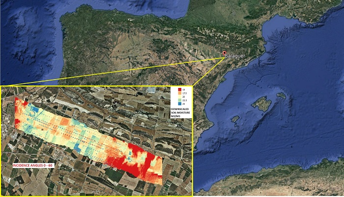
Figure 3.
Location of the experiment area in the north east of the Iberian peninsula, near Balaguer (41.9°N, 0.80°E), Lleida, Spain. Zoom shows the collected GNSS-R data strips in [dB].
Figure 3.
Location of the experiment area in the north east of the Iberian peninsula, near Balaguer (41.9°N, 0.80°E), Lleida, Spain. Zoom shows the collected GNSS-R data strips in [dB].

Figure 4.
Experiment instrumentation: (a) CESSNA Caravan plane, (b) AISA (hyperspectral VNIR) and TASI (TIR), and (c) ARIEL L-band radiometer.
Figure 4.
Experiment instrumentation: (a) CESSNA Caravan plane, (b) AISA (hyperspectral VNIR) and TASI (TIR), and (c) ARIEL L-band radiometer.

Figure 5.
Normalized Difference Vegetation Index (NDVI) from Sentinel 2 L1C for October 23rd, 2018. Yellow rectangle corresponds to the second quadrant of zoom region of Figure 3. North West corner: 41°47’33"N, 0°50’4"E; South East corner: 41°46’56"N, 0°51’57"E, distance = 2.9 km.
Figure 5.
Normalized Difference Vegetation Index (NDVI) from Sentinel 2 L1C for October 23rd, 2018. Yellow rectangle corresponds to the second quadrant of zoom region of Figure 3. North West corner: 41°47’33"N, 0°50’4"E; South East corner: 41°46’56"N, 0°51’57"E, distance = 2.9 km.

Figure 6.
Example showing the difference between Sentinel-2 NDVI and AISA narrowband NDVI (top), and AISA wideband NDVI (middle panel). Bottom panel shows the TASI thermal image in [°C]. Region corresponds to yellow rectangle in Figure 5.
Figure 6.
Example showing the difference between Sentinel-2 NDVI and AISA narrowband NDVI (top), and AISA wideband NDVI (middle panel). Bottom panel shows the TASI thermal image in [°C]. Region corresponds to yellow rectangle in Figure 5.

Figure 7.
Locations where the soil samples, in situ soil moisture measurements, and surface roughness profiles acquired (refer to Figure 3 and Figure 5).

Figure 8.
ARIEL-derived surface soil moisture downscaled to 0.8 m with the AISA NDVI and TASI (thermal data, land surface temperature (LST)), and some sample CORTO GNSS-R derived surface soil moisture (discussion on Soil Moisture retrieval in Section 3).
Figure 8.
ARIEL-derived surface soil moisture downscaled to 0.8 m with the AISA NDVI and TASI (thermal data, land surface temperature (LST)), and some sample CORTO GNSS-R derived surface soil moisture (discussion on Soil Moisture retrieval in Section 3).

Figure 9.
Sentinel-2 L1C Normalized Difference Water Index (NDWI) for October 23rd, 2018. Red rectangles correspond to regions in Figure 8.
Figure 9.
Sentinel-2 L1C Normalized Difference Water Index (NDWI) for October 23rd, 2018. Red rectangles correspond to regions in Figure 8.

Figure 10.
Sentinel-2 L1C Normalized Difference Water Index (NDWI) for October 23rd, 2018, and CORTO GNSS-R reflectivities. Red rectangles correspond to regions in Figure 8.
Figure 10.
Sentinel-2 L1C Normalized Difference Water Index (NDWI) for October 23rd, 2018, and CORTO GNSS-R reflectivities. Red rectangles correspond to regions in Figure 8.

Figure 11.
(a) Zoom of downscaled ARIEL SM map overlaid with CORTO GNSS-R SM measurements at the Balaguer airborne experiment site, incidence angles between 15° and 30° for October 22nd, 2018; and Sentinel-2 L1C (b) Normalized Difference Water Index (NDWI) and (c) NDVI for October 23rd, 2018. Region corresponds to left half of rectangle A in Figure 8, Figure 9 and Figure 10.


Figure 12.
Roughness parameter (square dots) [-] overlaid over the SM [m3/m3] map in the Region of Interest (ROI) (area corresponds to rectangle A in Figure 7, Figure 8 and Figure 9).

Figure 13.
Matched histograms of downscaled ARIEL SM values (blue), and CORTO GNSS-R-derived values (brown).
Figure 13.
Matched histograms of downscaled ARIEL SM values (blue), and CORTO GNSS-R-derived values (brown).

Figure 14.
Reflectivity [dB] and ad hoc surface roughness compensation for different incidence angles.
Figure 14.
Reflectivity [dB] and ad hoc surface roughness compensation for different incidence angles.

Figure 15.
Vegetation compensation [dB] (Equation (1)) for different incidence angles.

Figure 16.
Sample high GNSS-R reflectivity (calibrated for instrumental effects) over the forested area that is overcompensated for vegetation attenuation effects, or areas in which there is likely a variation in the subsurface soil moisture.
Figure 16.
Sample high GNSS-R reflectivity (calibrated for instrumental effects) over the forested area that is overcompensated for vegetation attenuation effects, or areas in which there is likely a variation in the subsurface soil moisture.

Figure 17.
Histograms of ARIEL (brown) and GNSS-R (blue) retrieved SM using surface roughness correction as a function of the incidence angles: (a) from 0° to 15°, (b) from 15° to 30°, (c) from 30° to 45°, and (d) from 45° to 60°.
Figure 17.
Histograms of ARIEL (brown) and GNSS-R (blue) retrieved SM using surface roughness correction as a function of the incidence angles: (a) from 0° to 15°, (b) from 15° to 30°, (c) from 30° to 45°, and (d) from 45° to 60°.

Figure 18.
ARIEL and GNSS-R retrieved SM, as a function of the incidence angle in steps of 15°: 1) 0°–15°, 2) 15°–30°, 3) 30°–45°, and 4) 45°–60°. Figures (a) and (b) correspond to rectangles A and B in Figure 8, Figure 9 and Figure 10. Note that after a regional calibration of roughness effects, values are much more similar (<5%), and that errors are larger in the 30°–45°, and 45°–60° ranges (larger color disagreement).


Figure 19.
ARIEL downscaled and CORTO GNSS-R retrieved SM: all incidence angles included.

© 2020 by the authors. Licensee MDPI, Basel, Switzerland. This article is an open access article distributed under the terms and conditions of the Creative Commons Attribution (CC BY) license (http://creativecommons.org/licenses/by/4.0/).
Share and Cite
MDPI and ACS Style
Camps, A.; Park, H.; Castellví, J.; Corbera, J.; Ascaso, E. Single-Pass Soil Moisture Retrievals Using GNSS-R: Lessons Learned. Remote Sens. 2020, 12, 2064. https://0-doi-org.brum.beds.ac.uk/10.3390/rs12122064
AMA Style
Camps A, Park H, Castellví J, Corbera J, Ascaso E. Single-Pass Soil Moisture Retrievals Using GNSS-R: Lessons Learned. Remote Sensing. 2020; 12(12):2064. https://0-doi-org.brum.beds.ac.uk/10.3390/rs12122064
Chicago/Turabian StyleCamps, Adriano, Hyuk Park, Jordi Castellví, Jordi Corbera, and Emili Ascaso. 2020. "Single-Pass Soil Moisture Retrievals Using GNSS-R: Lessons Learned" Remote Sensing 12, no. 12: 2064. https://0-doi-org.brum.beds.ac.uk/10.3390/rs12122064
Note that from the first issue of 2016, this journal uses article numbers instead of page numbers. See further details here.